First case of strong gravitational lensing by a QSO : SDSS J0013+1523 at z = 0.120

We present the first case of strong gravitational lensing by a QSO : SDSS J0013+1523at $z=0.120$. The discovery is the result of a systematic search for emission lines redshifted behind QSOs, among 22 298 spectra of the SDSS data release 7. Apart from the $z=0.120$ spectral features of the foreground QSO, the spectrum of SDSS J0013+1523  also displays the [O II] and H$\beta$ emission lines and the [O III] doublet, all at the same redshift, $z=0.640$. Using sharp Keck adaptive optics K-band images obtained using laser guide stars, we unveil two objects within a radius of 2″ from the QSO. Deep Keck optical spectroscopy clearly confirms one of these objects at $z=0.640$ and shows traces of the [O III]  emission line of the second object, also at $z=0.640$. Lens modeling suggests that they represent two images of the same $z=0.640$ emission-line galaxy. Our Keck spectra also allow us to measure the redshift of an intervening galaxy at $z=0.394$, located 3.2″  away from the line of sight to the QSO. If the $z=0.120$ QSO host galaxy is modeled as a singular isothermal sphere, its mass within the Einstein radius is $M_{E}(r<1\,h^{-1}\,kpc)=2.16\times 10^{10}\ h^{-1}\ M_{\odot}$ and its velocity dispersion is $\sigma_{\rm SIS}=169$ km s^-1. This is about 1-$\sigma$ away from the velocity dispersion estimated from the width of the QSO H$\beta$ emission line, $\sigma_{*}(M_{BH})=124\pm 47$ km s^-1. Deep optical HST imaging will be necessary to constrain the total radial mass profile of the QSO host galaxy using the detailed shape of the lensed source. This first case of a QSO acting as a strong lens on a more distant object opens new directions in the study of QSO host galaxies.

1 Introduction

With the growing number of ongoing and future wide-field surveys, strong gravitational lensing is becoming a powerful tool to weigh individual galaxies and study their total radial mass profiles. Historically, strong lenses have long been source-selected, i.e., they were found by identifying gravitationally lensed multiple images of distant sources such as QSOs, either in the optical (e.g., SDSS; Oguri et al. OGU06 (2006)) or in the radio (e.g., the CLASS survey; e.g., Browne et al. BROWN03 (2003), Myers et al. MYERS03 (2003)). The discoveries of multiply imaged QSOs, by numerous independent teams over two decades, have led to a sample of about 100 strongly lensed QSOs. Detailed HST imaging is now available for most of these objects mainly thanks to the CfA-Arizona Space Telescope LEns Survey (CASTLES; Muñoz et al.MUN98 (1998), Impey et al. IMP98 (1998)). The second largest sample of source-selected systems is the one obtained in the COSMOS field (Faure et al. FAU (2008)), where the sources are almost always emission-line galaxies.

Source-selected samples tend to yield lensing galaxies spanning a broad range of physical properties, i.e., effective radii, Einstein radii, dark matter profiles, total masses, and environments. With current wide-field surveys such as the SDSS, it is now also possible to build lens-selected samples, where the lenses can be chosen with well-defined photometric properties. The largest sample of these lens-selected systems to date is the SLACS sample (e.g., Bolton et al. BOL (2008)), where the lenses are color-selected early-type galaxies with $0.1<z<0.6$ and where the sources are emission line galaxies with $z>0.5$. While source-selected samples use optical or radio data to look for multiple images, SLACS uses SDSS optical spectra to look for emission lines redshifted behind the selected lensing galaxies, following the technique of Warren et al. (WAR (1996)).

Figure 1: Top: SDSS spectrum of SDSS J0013+1523, after subtraction of the continuum, as provided by the SDSS pipeline. The emission lines associated with the foreground $z=0.120$ QSO are shown with vertical dotted lines (black) and the emission lines associated with the $z=0.640$ background object are shown with dashed lines (red). The noise spectrum is also displayed indicating the position of the strongest sky lines. Bottom: from left to right, zooms on the $z=0.640$ [O II], H$\beta$ and on the [O III]  doublet. The noise spectrum does not show any strong feature at the position of the background emission lines. Note as well that the [O II]  doublet is spectrally resolved. No smoothing has been applied.

Following the same approach, we started to compile a lens-selected sample where the foreground lenses are QSOs in place of early-type galaxies. Our long-term goal is to provide a direct measure of the total mass of QSO host galaxies and to use SLACS as a non-QSO “control” sample. Because the lensing QSOs are at low redshift ($z<0.4$), the range of follow-up applications is very rich, as their H$\beta$, H$\alpha$, [O III]  emission lines are clearly measurable in the SDSS spectra. In addition, the angular size and luminosity of their host galaxies make it possible to carry out direct spectroscopy of the host (e.g., Lewate et al. LETAW07 (2007), Letawe et al. LETAW04 (2004), Courbin et al. COU02 (2002)). Our sample will therefore allow us to test directly the scaling laws established between the properties of QSO emission lines, the mass of the central black hole, and the total mass of the host galaxies (e.g., Kaspi et al. KAS (2005), Bonning et al. BON (2005), Shen et al. SHEN (2008)).

In this paper, we focus on the discovery of the first case of a QSO, SDSS J0013+1523  (RA(2000): 00h 13m 40.21s; DEC(2000): +15^∘ 23′  12.1″; $z=0.120$; $r=18.04$), producing two images of a background galaxy ($z=0.640$) due to strong gravitational lensing.

Figure 2: Full field of view of the Keck NIRC2+AO observations. No star is available to construct the PSF. Also indicated are galaxies G1 and G2, which may contribute to the external shear of the lens models. From our Keck spectra, galaxy G2 is at $z=0.394$. North is to the top, east left.

2 Spectroscopic search in SDSS

We used the SDSS DR7 catalogue (Abazajian et al. ABA09 (2009)) of spectroscopically confirmed QSOs to build a sample of potential lenses, without applying any magnitude cut. We considered all QSOs in the catalogue with $0<z_{l}<0.7$, providing a sample of 22 298 potential lenses with SDSS spectra. In these spectra, we look for emission lines redshifted beyond the redshift of the QSO. Since the SDSS fiber is comparable in size (3″  in diameter) to the typical Einstein radius of our QSOs, the object responsible for the background emission lines is very likely to be strongly lensed (e.g., Bolton et al. BOL (2008)).

Figure 3: Left: zoom on the central part of Fig. 2. The resolution is 0.1″  FWHM and the pixel scale is 0.0397″. Two objects, labelled A and B, appear in the vicinity of the QSO. Middle: residual after subtraction of the GALFIT model (Moffat+exponential disk), where objects A and B are now well visible. The circle indicates the position of the QSO. Its size, 0.5″  in diameter, corresponds to the region where the subtraction may not be reliable, mainly due to the presence of the complex first Airy ring of the PSF. Spike-like features in the PSF are indicated by the dashed lines. Right: as in the middle panel, but a symmetrized PSF has been subtracted. This removes more effectively the Airy ring than an analytical model of the PSF.

Looking for emission lines in the background of QSOs is far more difficult than behind galaxies, for three reasons: (i) the QSO outshines the lensed background images, making follow-up imaging very challenging and (ii) in contrast to early-type galaxies, QSO spectra span a huge range of properties, both in the continuum and emission lines. It is therefore impossible to subtract a QSO template from the SDSS spectra and to search for emission lines in the residual spectrum. Finally, (iii), QSO spectra have many weak iron features that can mimic faint background emission lines. These lines lead to false positives that can be removed statistically thanks to the huge number of QSO spectra available in SDSS.

Although our search technique will be the topic of a future paper, the main components of our strategy are the following. First we subtract the continuum of the QSO spectra using a spline fit. Then, we cross-correlate the continuum-subtracted spectra with several analytical templates of emission lines. We typically use 3 templates, one with only the optical H$\beta$ and [O III]  doublet, a second to which we add the [O II]  doublet, and a third that also contains H$\alpha$. The cross-correlation provides us with a catalogue of candidates, a candidate being defined as a significant peak in the cross-correlation function of redshift higher than the foreground QSO. Each QSO spectrum has many possible candidates, of which we retain the 5 most significant. For those, we fit Gaussian profiles to each of the candidate emission lines and compute a quality factor, based on the total signal-to-noise ratio (S/N) in the spectroscopic lines.

The quality factor is used to select the most likely candidates in terms of S/N. However, at this point, the catalogue of candidates still needs to be cleaned from false positives produced by residuals caused by either sky subtraction or faint features in the spectrum of the foreground QSO. Thanks to the large number of QSOs in the SDSS sample, these can be identified statistically and rejected efficiently. As a final step, we carry out a visual inspection of the most probable candidates. This process leaves us with about 10 candidates that have at least 3 significant emission lines and an additional 4 candidates with 4 emission lines. SDSS J0013+1523  is one of the latter. Its SDSS spectrum and the background emission lines at $z_{s}=0.640$ are shown in Fig. 1.

If all 14 objects are actually lensed, the probability of finding these objects is $14/22,298=6.2\times 10^{-4}$. This is about 8 times less than in SLACS, where the discovery rate is 0.005 (e.g., Auger et al. AUGER09 (2009)). However, our selection function is very different from SLACS, because of (i) the contrast between the QSO and the background emission lines, (ii) the regions of the QSO spectra that must be masked due to strong QSO spectral features, (iii) the requirement to see multiple background emission lines simultaneously outside the masked regions, (iv) differences between the redshift distributions of QSOs in our sample and the galaxies in SLACS. A detailed study of the selection function (e.g., Dobler et al. DOB08 (2008)) beyond the scope of the present discovery paper. However, if real, the difference between the SLACS discovery rate and ours may reflect a genuine difference between the lensing cross-sections of the two samples, i.e., between the physical properties of QSO and non-QSO galaxies.

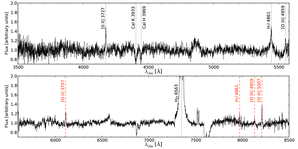
Figure 4: Keck/LRIS spectrum of SDSS J0013+1523, normalized to the continuum. As in Fig. 1, the labels in black show the spectral features associated with the foreground $z=0.120$ QSO and the labels in red show the emission lines of the $z=0.640$ background galaxy. No smoothing has been applied.

3 Keck adaptive optics imaging

The imaging observations were obtained on the night of 11 September 2009 UT, using the NIRC2 instrument in the laser guide star adaptive optics mode (LGSAO; Wizinowitch et al. 2006) at the 10-m Keck-2 telescope on Mauna Kea, Hawaii, in variable conditions. Images were obtained in the $K^{\prime}$ band, using the “wide field” NIRC2 camera with the FOV $\approx$ 40 arcsec, and the pixel scale of 0.0397″. The observations consist of 42 dithered exposures of 40 seconds each. The data were reduced using standard procedures, leading to the combined image shown in Fig. 2.

Owing to the small field of view of the NIRC2+AO imager, no star is available to construct a numerical point spread function (PSF), hence making image deconvolution impossible. We nevertheless subtracted the low spatial frequencies of the PSF in two different ways.

First, we used the GALFIT package (Peng PEN02 (2002)) to fit analytical profiles to the data. We tried a number of different models where the QSO is represented with either a Gaussian or a Moffat profile and where the host galaxy is represented by an elliptical Sersic, a de Vaucouleurs, or an exponential disk profile. We found that the best fits were thoses with a Moffat for the QSO and an exponential disk for the host. This model was subtracted from the 42 individual images and the difference images were then stacked and cleaned for cosmic-rays using sigma-clipping.

As a second method, we computed an estimate of the PSF directly from the QSO itself. The goal here was to remove the low frequency signal of the PSF (plus QSO host galaxy), by symmetrizing the image of the QSO. For each of the 42 frames, we produced 10 different duplicates rotated by 36 degrees about the QSO centroid. We then took the median of these 10 rotated frames, hence producing a circularly symmetric PSF. Thanks to the median average, all small details in the PSF were removed, i.e., the spikes, any blob in the PSF, and the putative lensed images of a background object. The 42 PSFs were then subtracted from the data and the residual images were stacked together.

Table 1: Summary of the Keck astrometry. The error bars in the positions are about 20 mas, i.e., about half a pixel.

Object	$x$(″)	$y$(″)	Flux
QSO	$+$0.000	$+$0.000	$-$
A	$+$0.731	$+$0.027	1.00
B	$-$0.539	$+$0.132	0.72
G1	$-$8.318	$+$2.873	$-$
G2	$-$2.842	$+$1.610	$-$

The results of these two ways of subtracting the QSO are shown in Fig. 3. The subtraction is found satisfactory for distances larger than 0.25″ away from the QSO. In this area, the structures in the PSF-subtracted data change depending on the model we adopt in GALFIT. This is because the first diffraction ring of the PSF that cannot be modeled analytically. This ring is more accurately modeled by our second subtraction method, where we symmetrized the PSF.

Two obvious objects are found to the east and west of the QSO, labelled A and B in Fig. 3. These are outside the area where the PSF subtraction is uncertain and they are not located on the PSF spikes indicated by dashed lines in the middle panel of Fig. 3. We consider them as the best candidates for lensed images of a source at $z_{s}=0.640$. All other faint structures are either superimposed with PSF features or are not fitted by lens models (Sect. 5). A summary of the relative astrometry and the flux ratio of objects A to B is given in Table 1.

4 Keck optical spectroscopy

Deep Keck optical spectra were obtained on the night of 20 December 2009, using the LRIS instrument (Oke et al. OKE95 (1995)). The weather conditions were variable, with patchy clouds. The seeing at the moment of the observations was 1.5″.

A long slit was used (1.5″ wide), with a position angle (PA) of 70^∘, ensuring that we could observe simultaneously the QSO as well as object A and galaxy G2. Object B also enters partly in the slit. The data consist of 3 exposures of 600 seconds each, with nodding along the slit to minimize the effect of CCD traps. The wavelength range from 3500 Å  to 8500 Å  is covered using the dichroic #560 that splits the beam into a blue and a red channels. The spectrum in the blue channel is obtained using a 400 lines/millimeter grism and the spectrum in the red channel is obtained with a 600 lines/millimeter grism.

The data were reduced using the IRAF package, to perform the wavelength calibration, the sky subtraction, and the spectra combination in two dimensions. The pixel size in the blue channel is 0.6Å  in the spectral direction and 0.135″  in the spatial direction. In the red channel the spectral scale is 0.8 Å  per pixel and the spatial scale is 0.210″  per pixel. The final 1D spectrum was extracted, confirming all of the $z=0.640$ emission lines seen in the SDSS spectrum (Fig. 4). In addition to the QSO spectrum we also obtained the spectrum of galaxy G2, allowing us to measure its redshift from the [O II], H$\beta$, and [O III]  emission lines, $z=0.394$. This rules out the possibility that G2 is a counter image of object A. We do not detect the continuum of G2.

The seeing for the 2D spectra was poor, but sufficient to separate spatially the spectrum of the QSO from that of object A. This was achieved by subtracting a two-dimensional Moffat profile from the data, clearly unveiling the four $z=0.640$ emission lines seen in the 1D spectrum, off-centered by 0.8″  from the centroid of the QSO. This is almost exactly the separation betwen the QSO and object A. We show in Fig. 5 the result of the QSO subtraction for the two brightest emission lines. Although the signal is very weak, we can also detect a weak [O III]  emission line at the position expected for object B. Deeper observations with better seeing would be needed to provide firm conclusions.

Figure 5: Two-dimensional spectrum of SDSS J0013+1523  obtained with the Keck and LRIS. The spatial direction runs along the x-axis and the spectral direction along the y-axis (red to the top). Top: zoom on the [O III] (5007Å) emission line, redshifted to $z=0.640$. The left panel shows the original spectrum, while the right panel shows the data after subtraction of the QSO spatial profile, centered on the dashed line. Object A is clearly detected, off-center with respect to the QSO, and traces of B may be present at the position expected from the AO images. Bottom: same as above but for the [O II] (3727 Å) doublet.

5 Lens modeling

We show that the observed image configuration is consistent with the gravitational lens hypothesis. We model the mass distribution of the lens with a singular isothermal sphere (SIS) and include the effect of the environment as an external shear. This simple model has three parameters: the angular Einstein radius $\theta_{E}$ of the SIS, the amplitude $\gamma$, and the position angle $\theta_{\gamma}$ of the shear. The observational quantities used to constrain the model are the relative positions of the lensed images A and B and the flux ratio of these images. Since the flux ratio can be affected by differential extinction, PSF uncertainties, or microlensing, we assume an error of up to 20% in the flux ratio reported in Table 1. The center of the SIS is assumed to be coincident with the position of the lensing QSO. Using the lensmodel lensing code developed by Keeton (2001), we find that the observed system can be perfectly reproduced ($\chi^{2}\sim$ 0) with the following model parameters ($\theta_{E}$, $\gamma$, $\theta_{\gamma}$) = (0.64$\pm$0.06$\arcsec$, 0.019$\pm$ 0.02, 43${}^{+6}_{-4}$).

The angular Einstein radius $\theta_{E}$ of the SIS model is directly related to the central velocity dispersion $\sigma_{SIS}$of the stars in the galaxy by the equation

$$\theta_{E}=\frac{4\pi\sigma_{SIS}^{2}}{c^{2}}\frac{D_{ls}}{D_{os}},$$ (1)

where $D_{ls}$ (respectively $D_{os}$) is the angular cosmological distance between the lens and the source (resp. observer and source). Using this formula, we find $\sigma_{SIS}\sim$ 169 km s^-1 for our best model. Because multiple images are observed, the surface mass density $\Sigma$ inside the Einstein radius equals the critical surface mass density $\Sigma_{c}$. This allows us to calculate the amount of mass $M_{E}$ inside the Einstein radius $R_{E}=1\,h^{-1}$ kpc. We find $M_{E}=2.16\times 10^{10}\ h^{-1}\ M_{\odot}$. This mass might be overestimated as the intervening galaxies G1 and G2 are not included in the lens modeling, due to the lack of sufficient observational constraints (such as the masses of G1 and G2). However, Keeton & Zabludoff (KEEZAB04 (2004)) show that this overestimate is unlikely to be larger than 6%. This would result in an overestimate of 3% in the velocity dispersion, i.e., only 5 km s^-1.

We can compare $\sigma_{SIS}$ to two estimates of the velocity dispersion based on the SDSS spectrum of SDSS J0013+1523. Shen et al. (SHEN (2008)) measure the stellar velocity dispersion of the host galaxy, based on the broadening of absorption features observed its spectrum. They derive a surprisingly small value, $\sigma_{*}=96.4\pm 13.8$ km s^-1. We note, however, that this value is based on a low S/N spectrum of the host galaxy, following a principle component analysis decomposition of the SDSS spectrum. While this is certainly sufficient to measure, statistically, velocity dispersions for a large sample of objects, the accuracy reached for individual objects remains limited.

An indirect but more robust estimate of $\sigma_{*}$ can be found using the relation between the black hole mass and the galaxy velocity dispersion derived by Gültekin et al. (GUL (2009)) for all type of host galaxies. Using the black hole mass estimate $log(M_{BH})=7.24\pm 0.27$ M_⊙ derived by Shen et al. (SHEN (2008)) from the width of the H$\beta$ emission line of the QSO, we obtain $\sigma_{*}(M_{BH})=124\pm 47$ km s^-1. We note that the width of the QSO H$\beta$ line measured by Shen et al. (SHEN (2008)), FWHM(H$\beta$) $\sim$ 2920 $\pm$ 390 km s^-1, compares well with our measurement from the Keck spectra: FWHM(H$\beta$) $\sim$ 3090 km s^-1. The error associated with the former estimate is derived by adding quadratically the intrinsic scatter in the error in the black hole mass and by propagating the various errors in the formula of Gültekin et al. (GUL (2009)). The latter estimate is, within 1$\sigma$, compatible with the lensing velocity dispersion.

6 Conclusions

We have conducted a systematic spectroscopic search for QSOs acting as strong gravitational lenses on background emission-line galaxies. This has produced a sample of about 14 potential lenses.

We have presented Keck-AO imaging of one of the most likely candidates, SDSS J0013+1523, a QSO at $z=0.120$ whose spectrum additionally displays four emission lines at the same redshift, $z=0.640$. After PSF subtraction, we found two faint objects, A and B, within a radius of 2″ from the QSO.

Keck LRIS spectroscopy of SDSS J0013+1523  spatially resolves object A and confirms that it is at $z=0.640$. Traces of object B may be seen at the expected position, also at $z=0.640$. We measured the redshift of one of the two galaxies seen in the vicinity of the QSO, galaxy G2 at $z=0.394$.

The position, flux ratio, and shape of objects A and B are fully compatible with simple lens models involving a singular isothermal sphere plus external shear. Although lower than in most galaxies in SLACS, the velocity dispersion found from the lens models is within 1$\sigma$ compatible with that estimated from the empirical scaling laws established between the mass of the central black-hole and that of the QSO host galaxy.

Given the available observations, SDSS J0013+1523  is the first example of strong gravitational lensing by a QSO. Full confirmation will require deep HST observations in the optical, where the emission lines of the background object are prominent.

Apart from the exotic nature of SDSS J0013+1523, the discovery may open a new direction in the study of QSOs, providing a powerful test of existing empirical scaling laws in QSOs and allowing us to measure the total radial mass profile of QSO host galaxies with unprecedented accuracy.

- (1) Abazajian, K.N., Adelman-McCarthy, J.K., Agüeros, M.A., et al. 2009, ApJS, 182, 543
- (2) Auger, M.W., Treu, T., Bolton, A.S., et al. 2009, ApJ, 705, 1099
- (3) Bolton, A.S., Burles, S., Koopmans, L.V.E., et al. 2008, ApJ, 682, 964
- (4) Bonning, E.W., Shields, G.A., Salviander, S., McLure, R.J., 2005, ApJ, 626, 89
- (5) Browne, I. W. A., Wilkinson, P. N., Jackson, N. J. F., et al. 2003, MNRAS, 341, 13
- (6) Courbin, F., Letawe, G., Magain, P., et al. 2002, A&A, 394, 863
- (7) Dobler, G., Keeton, C.R., Bolton, A.S., Burles, S., 2008, ApJ, 685, 57
- (8) Faure, C., Kneib, J.-P., Covone, G., et al. 2008, ApJS, 176, 19
- (9) Gültekin, K., Richstone, D.O., Gebhardt, K., et al. 2009, ApJ, 698, 198
- (10) Impey, C. D., Falco, E. E., Kochanek, C. S., et al. 1998, ApJ, 509, 551
- (11) Kaspi, S., Maoz, D., Netzer, H., 2005, ApJ, 629, 61
- (12) Keeton C. R., 2001, astro-ph/0102341
- (13) Keeton, C. S., Zabludoff, A.I., 2004, ApJ, 612, 660
- (14) Letawe, G., Courbin, F., Magain, P., et al. 2004, A&A, 424, 455
- (15) Letawe, G., Courbin, F., Magain, P., et al. 2007, MNRAS, 378, 83
- (16) Muñoz, J. A., Falco, E. E., Kochanek, C. S., et al. 1998, Ap&SS, 263, 51
- (17) Myers, S. T., Jackson, N. J., Browne, I. W. A., et al. 2003, MNRAS, 341, 1
- (18) Oke, J.B., Cohen, J. G., Carr, M., et al. 1995, PASP, 107, 375
- (19) Oguri, M., Inada, N., Pindor, B., et al. 2006, AJ, 132, 999
- (20) Peng, C. Y., Ho, L. C., Impey, C. D., Rix, H.-W. 2002, AJ, 124, 266
- (21) Shen, J., Vanden Berk, D.E., Schneider, D.P., Hall, P.B., 2008, ApJ, 135, 928
- (22) Treu, T., Koopmans, L.V., Bolton, A.S., Burles, S., Moustakas, L.A. 2006, ApJ, 640, 662
- (23) Treu, T., Koopmans, L.V. 2004, ApJ, 611, 739
- (24) Warren, S. J., Hewett, P. C., Lewis, G. F., et al., 1996, MNRAS, 278, 139
- (25) Wizinowich, P., Le Mignant, D., Bouchez, A.H., et al. 2006, PASP, 118, 297