The $B_{s0}$ meson and the $B_{s0}BK$ coupling from QCD sum rules

Abstract

We evaluate the mass of the $B_{s0}$ scalar meson and the coupling constant in the $B_{s0}BK$ vertex in the framework of QCD sum rules. We consider the $B_{s0}$ as a tetraquark state to evaluate its mass. We get $m_{B_{s0}}=(5.85\pm 0.13)~{}\nobreak\,\mbox{GeV}$, which is in agreement, considering the uncertainties, with predictions supposing it as a $b\bar{s}$ state or a $B\bar{K}$ bound state with $J^{P}=0^{+}$. To evaluate the $g_{B_{s0}BK}$ coupling we use the three point correlation functions of the vertex, considering $B_{s0}$ as a normal $b\bar{s}$ state. The obtained coupling constant is: $g_{B_{s0}BK}=(16.3\pm 3.2)~{}\nobreak\,\mbox{GeV}$. This number is in agreement with light-cone QCD sum rules calculation. We have also compared the decay width of the $B_{s0}\to BK$ process considering the $B_{s0}$ to be a $b\bar{s}$ state and a $BK$ molecular state. The width obtained for the $BK$ molecular state is twice as big as the width obtained for the $b\bar{s}$ state. Therefore, we conclude that with the knowledge of the mass and the decay width of the $B_{s0}$ meson, one can discriminate between the different theoretical proposals for its structure.

I Introduction

In recent years the observation of heavy flavor hadrons have raised strong interest in interpreting these states as multiquark states, like tetraquarks states and hadronic molecules. Famous examples are the scalar $D_{s0}(2317)$ and the axial $D_{s1}(2460)$ charmed mesons, and the $X(3872)$ hidden charm meson. In the bottom sector, the recent observations of the $J^{P}=1^{+}$ $B_{s1}(5830)$ by the CDF collaboration cdf and the $J^{P}=2^{+}$ $B_{s2}(5840)$ by the CDF and D0 collaborations cdf ; d0 enrich the spectrum of the bottom-strange system and estimulate our interest in the possible interpretation of these states as multiquark states. In particular the yet unobserved $J^{P}=0^{+}$ $B_{s0}$ state, could be very broad and, therefore, very difficult to be observed, if it is a multiquark system with mass above the $BK$ threshold. There are already some predictions for the $B_{s0}$ mass supposing it is a $B\bar{K}$ bound state gscpz , as a $b\bar{s}$ state wang , and as a mixture between a $b\bar{s}$ and a $(bq)(\bar{s}\bar{q})$ states vvf . Although the structure for the $B_{s0}$ in these calculations is very different, the predictions for its mass are very similar: $(5.725\pm 0.039)~{}\nobreak\,\mbox{GeV}$ in ref. gscpz , $(5.70\pm 0.11)~{}\nobreak\,\mbox{GeV}$ in ref. wang and $5.68~{}\nobreak\,\mbox{GeV}$ in ref. vvf , for a state with 30% of the four-quark component.

There are also predictions for the $B_{s0}BK$ coupling constant, supposing the $B_{s0}$ to be a $B\bar{K}$ bound state gscpz and a $b\bar{s}$ state wang2 , and for the $B_{s0}B_{s}\pi$ coupling constant, supposing the $B_{s0}$ to be a $B\bar{K}$ bound state fglm . The knowledge of the coupling constant at the $B_{s0}BK$ vertex is very important since the decay width in this channel, the most important channel if it is allowed, can give an idea of the total width of the state. For one still unobserved state, it is very important for the experimentalists to have theoretical predictions not only about its mass, but also about its width. As an example, the mass of the scalar $D_{s0}(2317)$ meson is below the $DK$ threshold, therefore the decay $D_{s0}(2317)\to DK$ is not allowed. As a consequence, the $D_{s0}(2317)$ is very narrow since the main decay channel for this state is the isospin violating mode $D_{s0}(2317)\to D\pi$. The same could happen with the scalar $B_{s0}$ if its mass is bellow the $BK$ threshold. By the other hand, if its mass is above the $BK$ threshold, two scenarios are possible:

• it can be a very broad state if it is a tetraquark state, like the light scalars, since the decay $B_{s0}\to BK$ will be super allowed

• or it can still be narrow if it is a normal $b\bar{s}$ state, like the new recently observed states $B_{s1}(5830)$ and $B_{s2}(5840)$, if the coupling at the vertex $B_{s0}BK$ is not very large.

In the last case, the knowledge of the $B_{s0}BK$ coupling constant is indeed very important, and could help the experimentalists in the search for such state.

In this work we use the QCD sum rule (QCDSR) approach svz ; rry ; SNB to study the mass of the $B_{s0}$ supposing it is a tetraquark state in a diquark-antidiquark configuration, similar to the supposition made for the $D_{s0}(2317)$ scalar meson in ref. pec . We get a bigger mass as compared with predicitions supposing it as a $b\bar{s}$ state wang or a $B\bar{K}$ bound state gscpz but, considering the uncertainties, still compatible with these predictions. Since the mass obtained is above the $BK$ threshold, as explained above, a tetraquark scalar $B_{s0}$ will be very broad and, therefore, very difficult to be observed.

Since the prediction for the mass of $B_{s0}$, supposing it is a normal $b\bar{s}$ state: $(5.70\pm 0.11)~{}\nobreak\,\mbox{GeV}$ wang , can be above the $BK(5774)$ threshold, as explained above, it is very important to know the $B_{s0}BK$ coupling constant, therefore, in this work we also evaluate the $B_{s0}BK$ coupling constant supposing the $B_{s0}$ to be a normal $b\bar{s}$ state.

This paper is organized as follows: in Sec. II we introduce the two-point function to evaluate the mass of the tetraquark state. In Sec. III we study the three-point function for the $B_{s0}BK$ vertex. In Sec. IV we present our conclusions.

II Sum rule for the mass of the $B_{s0}$ scalar meson

In the QCDSR approach, the short range perturbative QCD is extended by an OPE expansion of the correlator, which results in a series in powers of the squared momentum with Wilson coefficients. The convergence at low momentum is improved by using a Borel transform. The expansion involves universal quark and gluon condensates. The quark-based calculation of a given correlator is equated to the same correlator, calculated using hadronic degrees of freedom via a dispersion relation, providing sum rules from which a hadronic quantity can be estimated.

Considering the $B_{s0}$ scalar meson as a $S$-wave bound state of a diquark-antidiquark pair, and considering the diquark in a spin zero colour anti-triplet, a possible current describing such state is given by:

$$j={\epsilon_{abc}\epsilon_{dec}\over\sqrt{2}}\left[(u_{a}^{T}C\gamma_{5}b_{b})(\bar{u}_{d}\gamma_{5}C\bar{s}_{e}^{T})+(d_{a}^{T}C\gamma_{5}b_{b})(\bar{d}_{d}\gamma_{5}C\bar{s}_{e}^{T})\right],$$ (1)

where $a,~{}b,~{}c,~{}...$ are colour indices and $C$ is the charge conjugation matrix.

The QCDSR for the bottom-strange scalar meson is constructed from the two-point correlation function

$$\Pi(q)=i\int d^{4}x~{}e^{iq.x}\langle 0|T[j(x)j^{\dagger}(0)]|0\rangle.$$ (2)

In the OPE side we work at leading order in $\alpha_{S}$ and consider condensates up to dimension eight. We treat the strange quark as a light quark and consider the diagrams up to order $m_{s}$. In ref. jido it was shown that the $q\bar{q}$ annihilation diagrams are more important for the 4-quark correlators than for the normal 2-quark mesonic correlators. Therefore, the $q\bar{q}$ annihilation diagrams can not be neglected a priori. Also, due to these $q\bar{q}$ annihilation diagrams, the current in Eq. (1) can mix with a two-quark $b\bar{s}$ current. Mixed tetraquark two-quark currents were considered to the study of the light scalars oka24 and also for the study of the $X(3872)$ meson x24 ; report in the framework of QCDSR. In this work we will not consider the $q\bar{q}$ annihilation diagrams neither the mixed tetraquark two-quark current. Therefore, our calculation will provide only the 4-quark contributions to the 4-quark correlator in Eq. (2).

The correlation function in the OPE side can be written in terms of a dispersion relation:

$$\Pi^{OPE}(q^{2})=\int_{m_{b}^{2}}^{\infty}ds{\rho(s)\over s-q^{2}}\;,$$ (3)

where the spectral density is given by the imaginary part of the correlation function: $\rho(s)={1\over\pi}\mbox{Im}[\Pi^{OPE}(s)]$.

In the phenomenological side the coupling of the scalar $B_{s0}$ meson to the scalar current in Eq. (1) can be parametrized in terms of a parameter $\lambda$ as: $\langle 0|j|B_{s0}\rangle=\lambda$. Therefore, the phenomenological side of Eq. (2) can be written in terms of $\lambda$ as:

$$\Pi^{phen}(q^{2})={\lambda^{2}\over m_{B_{s0}}^{2}-q^{2}}+\cdots\;,$$ (4)

where the dots denote higher resonance contributions that will be parametrized, as usual, through the introduction of the continuum threshold parameter $s_{0}$ io1 .

After making a Borel transform on both sides, and transferring the continuum contribution to the OPE side, the sum rule for the scalar meson $B_{s0}$ can be written as

$$\lambda^{2}e^{-m_{B_{s0}}^{2}/M^{2}}=\int_{m_{b}^{2}}^{s_{0}}ds~{}e^{-s/M^{2}}~{}\rho(s)\;,$$ (5)

where $\rho(s)=\rho^{pert}(s)+\rho^{m_{s}}(s)+\rho^{\langle\bar{q}q\rangle}(s)+\rho^{\langle G^{2}\rangle}(s)+\rho^{mix}(s)+\rho^{\langle\bar{q}q\rangle^{2}}(s)+\rho^{\langle G^{3}\rangle}(s)$, with

$$\rho^{pert}(s)={1\over 2^{10}3\pi^{6}}\int_{\Lambda}^{1}d\alpha\left({1-\alpha\over\alpha}\right)^{3}(m_{b}^{2}-s\alpha)^{4},$$ (6)

$$\rho^{m_{s}}(s)=0$$ (7)

$$\rho^{\langle\bar{q}q\rangle}(s)={1\over 2^{6}\pi^{4}}\int_{\Lambda}^{1}d\alpha~{}{1-\alpha\over\alpha}(m_{b}^{2}-s\alpha)^{2}\bigg{[}-\langle\bar{q}q\rangle\left(2m_{s}+m_{b}{1-\alpha\over\alpha}\right)+m_{s}\langle\bar{s}s\rangle\bigg{]},$$ (8)

$$\rho^{\langle G^{2}\rangle}(s)={\langle g^{2}G^{2}\rangle\over 2^{10}\pi^{6}}\int_{\Lambda}^{1}d\alpha~{}(m_{b}^{2}-s\alpha)\left[{m_{b}^{2}\over 9}\left({1-\alpha\over\alpha}\right)^{3}+(m_{b}^{2}-s\alpha)\left({1-\alpha\over 2\alpha}+{(1-\alpha)^{2}\over 4\alpha^{2}}\right)\right],$$ (9)

$$\rho^{\langle G^{3}\rangle}(s)={\langle g^{3}G^{3}\rangle\over 2^{12}9\pi^{6}}\int_{\Lambda}^{1}d\alpha\left({1-\alpha\over\alpha}\right)^{3}(3m_{b}^{2}-s\alpha),$$ (10)

$$\rho^{mix}(s) = {1\over 2^{6}\pi^{4}}\int_{\Lambda}^{1}d\alpha~{}(m_{b}^{2}-s\alpha)\bigg{[}-{m_{s}\langle\bar{s}g\sigma.Gs\rangle\over 6}+\langle\bar{q}g\sigma.Gq\rangle\bigg{(}-m_{s}(1-\ln(1-\alpha))$$ (11)

$$- m_{b}{1-\alpha\over\alpha}\left(1-{1-\alpha\over 2\alpha}\right)\bigg{)}\bigg{]}$$

$$\rho^{\langle\bar{q}q\rangle^{2}}(s)=-{\langle\bar{q}q\rangle\over 24\pi^{2}}\left[\langle\bar{s}s\rangle\left(2m_{b}^{2}-s-{m_{b}^{4}\over s}\right)+m_{s}m_{b}\left(\langle\bar{s}s\rangle-2\langle\bar{q}q\rangle\right)\left(1-{m_{b}^{2}\over s}\right)\right].$$ (12)

The lower limit of the integrations is given by $\Lambda=m_{b}^{2}/s$.

II.1 Results for the mass

In the numerical analysis of the sum rules, the values used for the quark masses and condensates are SNB ; SNCB ; narpdg ; SNG : $m_{s}=0.13\,\nobreak\,\mbox{GeV}$, $m_{b}(m_{b})=(4.24\pm 0.06)\,\nobreak\,\mbox{GeV}$, $\langle\bar{q}q\rangle=\,-(0.23)^{3}\,\nobreak\,\mbox{GeV}^{3}$, $\langle\overline{s}s\rangle\,=0.8\langle\bar{q}q\rangle$, $\langle\bar{q}g\sigma.Gq\rangle=m_{0}^{2}\langle\bar{q}q\rangle$, $\langle\bar{s}g\sigma.Gs\rangle=m_{0}^{2}\langle\bar{s}s\rangle$ with $m_{0}^{2}=0.8\,\nobreak\,\mbox{GeV}^{2}$, $\langle g^{2}G^{2}\rangle=0.88~{}\nobreak\,\mbox{GeV}^{4}$ and $\langle g^{3}G^{3}\rangle=0.045~{}\nobreak\,\mbox{GeV}^{6}$.

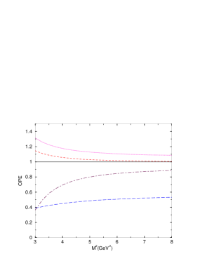
Figure 1: The OPE convergence for the $J^{P}=0^{+},~{}B_{s0}$ meson in the region $3\leq M^{2}\leq 8~{}\nobreak\,\mbox{GeV}^{2}$ for $\sqrt{s_{0}}=6.6$ GeV. We plot the relative contributions starting with the perturbative contribution (long-dashed line), and each other line represents the relative contribution after adding of one extra condensate in the expansion: + quark condensate (dashed line), + gluon condensate (dotted line), + mixed condensate (dot-dashed line), + four-quark condensate (solid line).

The Borel window is determined by analysing the OPE convergence, the Borel stability and the pole contribution. To determine the minimum value of the Borel mass we impose that the contribution of the higher dimension condensate should be smaller than 20% of the total contribution: $M^{2}_{min}$ is such that

$$\left|{\mbox{OPE summed up dim n-1 }(M^{2}_{min})\over\mbox{total contribution }(M^{2}_{min})}\right|=0.8.$$ (13)

In Fig. 1 we show the contribution of all the terms in the OPE side of the sum rule. From this figure we see that only for $M^{2}\geq 5.3$ GeV² the contribution of the dimension-6 condensate is around 20% of the total contribution. However, for such large value of the Borel mass there is no dominance of the pole contribution for $\sqrt{s_{0}}=6.6$ GeV. We interpret this as an indication that the dimension-6 condensate does not saturate the OPE. To improve the OPE convergence, we also include the dimension-8 condensate:

$$\rho^{D=8}(s) = {m_{0}^{2}\langle\bar{q}q\rangle\over 24\pi^{2}}\bigg{[}\langle\bar{s}s\rangle+{m_{s}m_{b}\over 4}\bigg{(}(4\langle\bar{q}q\rangle-ss)\int_{0}^{1}{d\alpha\over 1-\alpha}\delta\left(s-{m_{b}^{2}\over 1-\alpha}\right)-(4\langle\bar{q}q\rangle-2\langle\bar{s}s\rangle)\delta(s-m_{b}^{2})\bigg{)}\bigg{]}$$ (14)

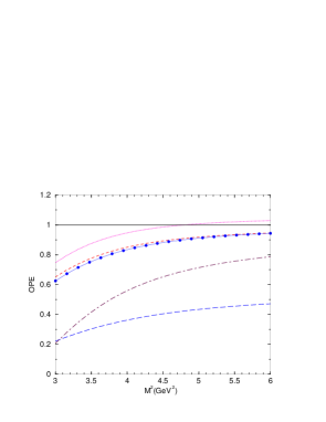
Figure 2: Same as Fig. 1 for $\sqrt{s_{0}}=6.7$ GeV: perturbative contribution (long-dashed line), + quark condensate (dashed line), + gluon condensate (dotted line), + mixed condensate (dot-dashed line), + four-quark condensate (solid line with dots)+ dimension-8 condensate (solid line).

From Fig. 2 we see that for $M^{2}\geq 4.0$ GeV² the contribution of the dimension-8 condensate is smaller than 20% of the total contribution. Therefore, the inclusion of the dimension-8 condensate improved the OPE convergence of the sum rule. We fix the lower value of $M^{2}$ in the sum rule window as $M^{2}_{min}=4.0$ GeV². One should note that a complete evaluation of higher dimension condensates contributions require more involved analysis including a non-trivial choice of the factorization assumption basis BAGAN . Therefore, in this work we do not consider condensates with dimension higher than 8.

The maximum value of the Borel mass is determined by imposing that the pole contribution must be bigger than the continuum contribution: $M^{2}_{max}$ is such that

$${\int_{m_{b}^{2}}^{s_{0}}ds~{}e^{-s/M^{2}_{max}}\rho(s)\over\int_{m_{b}^{2}}^{\infty}ds~{}e^{-s/M^{2}_{max}}\rho(s)}=0.5.$$ (15)

From a physical point of view, the continuum threshold parameter is related with the value of the mass of the first excited state, that has the same quantum numbers of the studied state. In general, the mass of the first excited state state is around 0.5 GeV above the mass of the low-lying state. Therefore, the continuum threshold can be related with the mass of the low-lying state, $H$, through the relation: $s_{0}\sim(m_{H}+0.5~{}\nobreak\,\mbox{GeV})^{2}$. To choose a good range of the values of $s_{0}$ we extract the mass from the sum rule, for a given $s_{0}$, and accept such value if the obtained mass is in the range 0.4 GeV to 0.6 GeV smaller than $\sqrt{s_{0}}$. Using this criterion, we obtain $s_{0}$ in the range $6.4\leq\sqrt{s_{0}}\leq 6.7$ GeV. However, for $\sqrt{s_{0}}=6.4~{}\nobreak\,\mbox{GeV}$ the allowed Borel region is very small, therefore, we only consider values of $\sqrt{s_{0}}$ in the range $6.5\leq\sqrt{s_{0}}\leq 6.7~{}\nobreak\,\mbox{GeV}$. We show in Table 1 the values of $M_{max}$ for different values of $\sqrt{s_{0}}$.

$\sqrt{s_{0}}~{}(\nobreak\,\mbox{GeV})$	$M^{2}_{max}(\nobreak\,\mbox{GeV}^{2})$
6.5	4.30
6.6	4.47
6.7	4.66

Table 1: Upper limits in the Borel window for the $0^{+},~{}B_{s0}$ meson obtained from the sum rule for different values of $\sqrt{s_{0}}$.

As pointed out in ref. jido , the determination of a sufficiently wide Borel window is the most important step for the application of the sum rule. In particular, without imposing correct criteria on the determination of the Borel window, artefacts as the appearance of pseudopeaks jido , could spoil the validity of the QCDSR results. As explained above we have used the two most important criteria to the determination of the Borel window: OPE convergence in Eq. (13) and pole contribution dominance in Eq. (15). Therefore, we do believe that the QCDSR studied here can be used to extract physical information about the $B_{s0}$ scalar meson.

The resonance mass, $m_{B_{s0}}$, can be obtained by taking the derivative of Eq. (5) with respect to $1/M^{2}$ and dividing it by Eq. (5):

$$m_{B_{s0}}^{2}={\int_{m_{b}^{2}}^{s_{0}}ds~{}e^{-s/M^{2}}~{}s~{}\rho(s)\over\int_{m_{b}^{2}}^{s_{0}}ds~{}e^{-s/M^{2}}~{}\rho(s)}\;.$$ (16)

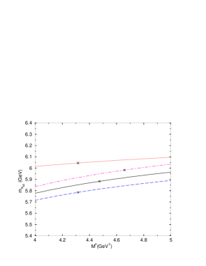
Figure 3: The $B_{s0}$ meson mass, described with a diquark-antidiquark current, as a function of the sum rule parameter ($M^{2}$) for $\sqrt{s_{0}}=6.5$ GeV (dashed line), $\sqrt{s_{0}}=6.6$ GeV (solid line) and $\sqrt{s_{0}}=6.7$ GeV (dot-dashed line). The dotted line shows the result obtained for the mass, for $\sqrt{s_{0}}=6.6$ GeV, considering only the condensates up to dimension 6. The crosses indicate the upper limits in the Borel region.

In Fig. 3 we show the obtained mass as a function of the Borel mass, for different values of $\sqrt{s_{0}}$. From this figure we see that the Borel stability is good in the allowed Borel window for all considered values of $s_{0}$. This is different from the case of the scalar charmed-strange meson $D_{s0}(2317)$, where no Borel window could be determined using the above mentioned criterious tetrarev . For completeness we also include in this figure (through the dotted line) the result obtained for the mass when considering only condensates up to dimension 6. We see that the inclusion of the dimension-8 condensates not only improves the OPE convergence but also reduces the mass of the state that couples with the current in Eq. (1).

Considering the variations on the quark masses, the quark condensate and on the continuum threshold discussed above, in the Borel window considered here our results for the ressonance mass is:

$$m_{B_{s0}}=(5.85\pm 0.13)~{}\nobreak\,\mbox{GeV},$$ (17)

which is compatible, considering the uncertainties, with the predictions from ref. gscpz : $(5.725\pm 0.039)~{}\nobreak\,\mbox{GeV}$, where the $B_{s0}$ is considered as a $B\bar{K}$ bound state, and from ref. wang : $(5.70\pm 0.11)~{}\nobreak\,\mbox{GeV}$, where the $B_{s0}$ is considered as a normal $b\bar{s}$ state.

Since we have not considered the $q\bar{q}$ annihilation diagrams in our calculation, the result in Eq. (17) gives only the 4-quark contribution to the mass of the $B_{s0}$. Therefore, the result in Eq. (17) is also in agreement with the findings in ref. vvf , where the authors have considered the $B_{s0}$ as being a mixture of $b\bar{s}$ and $(bq)(\bar{s}\bar{q})$ states. They find that the mass of the $B_{s0}$ state is smaller than the $BK$ threshold only when the four-quark componet is smaller than 30%. For a state where the four-quark component is dominante (51%) they get a mass $6.17~{}\nobreak\,\mbox{GeV}$.

Since the prediction for the mass of a $B_{s0}$ scalar meson with a dominante four-quark component is above the $BK$ threshold at 5774 MeV, the decay $B_{s0}\to BK$ will be super allowed for a $B_{s0}$ scalar meson with a dominante four-quark component. As a consequence such state will be very broad, like the light scalars, and very difficult to be observed. However, a two-quark state with a mass above the $BK$ threshold could still be narrow if the coupling at the $B_{s0}BK$ vertex is not very large. Therefore, in the next section we will evaluate the coupling at the $B_{s0}BK$ vertex, considering the $B_{s0}$ scalar meson as a $b\bar{s}$ state.

III The sum rule for the $B_{s0}BK$ vertex with $B_{s0}$ being a $b\bar{s}$ state

The coupling at the $B_{s0}BK$ vertex can be evaluated by using the three-point function QCDSR. Here we use the same technique developed in previous work for the evaluation of the couplings in the vetices $D^{*}D\pi$ nnbcs00 ; nnb02 , $DD\rho$bclnn01 , $DDJ/\psi$ mnns02 , $D^{*}DJ/\psi$ mnns05 , $D^{*}D^{*}\pi$ cdnn05 , $D^{*}D^{*}J/\psi$ bcnn05 , $D_{s}D^{*}K$, $D_{s}^{*}DK$ bccln06 , $DD\omega$ hmm07 , $D^{*}D^{*}\rho$ bcnn08 and $D_{sj}DK$ ko .

III.1 Sum rules for the form factors

The three-point function associated with the $B_{s0}BK$ vertex, for an off-shell $B$ meson, is given by

$$\Gamma_{\mu}^{(B)}(p,p^{\prime})=\int d^{4}x\,d^{4}y\;\;e^{ip^{\prime}\cdot x}\,e^{-i(p^{\prime}-p)\cdot y}\langle 0|T\{j_{\mu}^{K}(x)j^{B\dagger}(y)j^{B_{s0}\dagger}(0)|0\rangle,$$ (18)

and for an off-shell ${K}$ meson:

$$\Gamma_{\mu}^{({K^{0}})}(p,p^{\prime})=\int d^{4}x\,d^{4}y\;\;e^{ip^{\prime}\cdot x}\,e^{-i(p^{\prime}-p)\cdot y}\;\langle 0|T\{j^{B}(x)j_{\mu}^{K\dagger}(y)j^{B_{s0}\dagger}(0)\}|0\rangle\,.$$ (19)

The general expression for the vertices (18) and (19) has two independent Lorentz structures. We can write each $\Gamma_{\mu}$ in terms of the invariant amplitudes associated with each one of these structures in the following form:

$$\Gamma_{\mu}(p,p^{\prime})=F_{1}(p^{2},{p^{\prime}}^{2},q^{2})p_{\mu}+F_{2}(p^{2},{p^{\prime}}^{2},q^{2})p^{\prime}_{\mu},$$ (20)

where $q=p^{\prime}-p$.

Equations (18) and (19) can be calculated in two different ways: using quark degrees of freedom –the theoretical or OPE side– or using hadronic degrees of freedom –the phenomenological side.

The phenomenological side of the vertex function, $\Gamma_{\mu}(p,p^{\prime})$, is obtained by the consideration of $K$ and $B$ states contribution to the matrix element in Eqs. (18) and (19). The coupling at the vertex $B_{s0}BK$ is defined through the following effective Lagrangian

$$\mathcal{L}_{B_{s0}BK}=g_{B_{s0}BK}\Big{(}{\bar{B_{s0}}}\bar{B}K+B_{s0}B\bar{K}\Big{)},$$ (21)

from where one can deduce the matrix elements associated with the $B_{s0}BK$ momentum dependent vertices, that can be written it in terms of the form factors:

$$\langle B_{s0}(p)|K(p^{\prime})B(q)\rangle=g^{(B)}_{B_{s0}BK}(q^{2}),$$ (22)

and

$$\langle B_{s0}(p)|B(p^{\prime})K(q)\rangle=g^{(K)}_{B_{s0}BK}(q^{2}).$$ (23)

The meson decay constants, $f_{B_{s0}}$, $f_{B}$ and $f_{K}$, are defined by the following matrix elements:

$$\langle 0|j^{{B}_{s0}}|{B_{s0}(p)}\rangle=m_{B_{s0}}f_{B_{s0}};$$ (24)

$$\langle 0|j^{B}|{B(p)}\rangle=\frac{m^{2}_{B}}{m_{b}}f_{B}$$ (25)

and

$$\langle 0|j_{\nu}^{K}|{K(p)}\rangle=if_{K}p_{\mu},$$ (26)

Saturating Eqs. (18) and (19) with $B$ and $K$ states and using Eqs. (22), (23), (24), (25) and (26) we arrive at

$$\Gamma_{\mu}^{(B)phen}(p,p^{\prime})=g^{(B)}_{B_{s0}BK}(q^{2})\frac{f_{B_{s0}}f_{K}f_{B}\frac{m^{2}_{B}}{m_{b}}m_{B_{s0}}m_{K}}{(p^{2}-m^{2}_{B_{s0}})(q^{2}-m^{2}_{B})({p^{\prime}}^{2}-m^{2}_{K})}p^{\prime}_{\mu},$$ (27)

when the $B$ is off-shell, with a similar expression for the $K$ off-shell:

$$\Gamma_{\mu}^{(K)phen}(p,p^{\prime})=g^{(K)}_{B_{s0}BK}(q^{2})\frac{f_{B_{s0}}f_{B}f_{K}\frac{m^{2}_{B}}{m_{b}}m_{B_{s0}}m_{K}}{(p^{2}-m^{2}_{B_{s0}})(q^{2}-m^{2}_{K})({p^{\prime}}^{2}-m^{2}_{B})}q_{\mu}.$$ (28)

In the OPE or theoretical side the currents appearing in Eqs. (18) and (19) can be written in terms of the quark field operators in the following form:

$$j_{\mu}^{K}(x)=\bar{s}(x)\gamma_{\mu}\gamma_{5}u(x);$$ (29)

$$j^{B}(x)=i\bar{b}(x)\gamma_{5}u(x)$$ (30)

and

$$j^{B_{s0}}(x)=\bar{s}(x)b(x),$$ (31)

Each one of these currents has the same quantum numbers of the associated meson.

For each one of the invariant amplitudes appearing in Eq.(20), we can write a double dispersion relation over the virtualities $p^{2}$ and ${p^{\prime}}^{2}$, holding $Q^{2}=-q^{2}$ fixed:

$$F_{i}(p^{2},{p^{\prime}}^{2},Q^{2})=-\frac{1}{4\pi^{2}}\int_{s_{min}}^{\infty}ds\int_{u_{min}}^{\infty}du\>\frac{\rho_{i}(s,u,Q^{2})}{(s-p^{2})(u-{p^{\prime}}^{2})}\;,\;\;\;\;\;\;i=1,2$$ (32)

where $\rho_{i}(s,u,Q^{2})$ equals the double discontinuity of the amplitude $F_{i}(p^{2},{p^{\prime}}^{2},Q^{2})$, calculated using the Cutkosky’s rules.

We can work with any structure appearing in Eq.(20). However, since in Eq. (27) only the $p^{\prime}_{\mu}$ structure appears we choose to work with the $p^{\prime}$ structure. In order to reduce the influence of higher resonances and the pole-continuum transition constributions we perform a double Borel transform in both variables $P^{2}=-p^{2}\rightarrow M^{2}$ and ${P^{\prime}}^{2}=-{p^{\prime}}^{2}\rightarrow{M^{\prime}}^{2}$ and equate the two representations described above. We get the following sum rules:

$$\frac{m_{B_{s0}}m^{2}_{B}}{m_{b}}f_{K}f_{B}f_{B_{s0}}g^{(B)}_{B_{s0}BK}(Q^{2})e^{-m^{2}_{B_{s0}}/M^{2}}e^{-m^{2}_{K}/M^{{}^{\prime}2}}=(Q^{2}+m^{2}_{B})\,\,\bigg{[}m_{b}<\bar{s}s>e^{-m^{2}_{b}/M^{2}}$$

$$-\frac{1}{4\pi^{2}}\int_{m^{2}_{b}}^{s_{0}}ds\int_{0}^{u_{max}}\,du\exp(-s/M^{2})\exp(-u/M^{{}^{\prime}2})f(s,t,u)\theta(u_{0}-u)\bigg{]}$$ (33)

for an off-shell $B$, and

$$\frac{m_{B_{s0}}m^{2}_{B}}{m_{b}}f_{K}f_{B}f_{B_{s0}}g^{(K)}_{B_{s0}BK}(Q^{2})e^{-m^{2}_{B_{s0}}/M^{2}}e^{-m^{2}_{B}/M^{{}^{\prime}2}}$$ (34)

$$= -{Q^{2}+m^{2}_{K}\over 4\pi^{2}}\int_{m^{2}_{b}}^{s_{0}}ds\int_{u_{min}}^{u_{0}}\,due^{-s/M^{2}}e^{-u/M^{{}^{\prime}2}}g(s,t,u)$$

for an off-shell $K$.

In Eqs. (33) and (34), $t=-Q^{2}$,

$$f(s,t,u) = {3\over 2[\lambda(s,u,t)]^{1/2}}\left(m_{b}^{2}+2m_{b}m_{s}-s+\right.$$ (35)

$$+ \left.{(2m_{b}^{2}+2m_{b}m_{s}-s-t+u)(m_{b}^{2}(s-t+u)+s(t+u-s))\over\lambda(s,u,t)}\right),$$

$$g(s,t,u) = {3\over[\lambda(s,u,t)]^{3/2}}\left[m_{b}^{4}(s-t+3u)+u\left(m_{b}m_{s}(s+t-u)\right.\right.$$ (36)

$$+ \left.\left.s(-s+t+u)\right)+m_{b}^{2}\left(-2u(s-t+u)+m_{b}m_{s}(s-t+3u)\right)\right].$$

$\lambda(s,u,t)=s^{2}+u^{2}+t^{2}-2su-2st-2tu$, $u_{min}=m_{b}^{2}-{m_{b}^{2}t\over s-m_{b}^{2}}$ and $u_{max}=s+t-m_{b}^{2}-{st\over m_{b}^{2}}$.

Since we are dealing with heavy quarks, we expect the perturbative contribution to dominate the OPE. For this reason, we do not include the gluon and quark-gluon condensates in the present work.

In this work we use the following relations between the Borel masses $M^{2}$ and $M^{\prime 2}$: $\frac{M^{2}}{M^{\prime 2}}=\frac{m^{2}_{B_{s0}}-m_{b}^{2}}{0.64\nobreak\,\mbox{GeV}^{2}}$ for a $B$ off-shell and $\frac{M^{2}}{M^{\prime 2}}=\frac{m^{2}_{B_{s0}}}{m^{2}_{B}}$ for a $K$ off-shell.

III.2 Results for the form factors

$m_{b}(\nobreak\,\mbox{GeV})$	$m_{B_{s0}}(\nobreak\,\mbox{GeV})$	$m_{B}(\nobreak\,\mbox{GeV})$	$m_{K}(\nobreak\,\mbox{GeV})$	$f_{B_{s0}}(\nobreak\,\mbox{GeV})$	$f_{B}(\nobreak\,\mbox{GeV})$	$f_{K}(\nobreak\,\mbox{GeV})$	$\langle\bar{q}q\rangle(\nobreak\,\mbox{GeV})^{3}$
4.7	5.70	5.28	0.49	0.24	0.17	0.16	$(-0.23)^{3}$

Table 2: Parameters used in the calculation.

Table 2 shows the values of the parameters used in the present calculation. We take $f_{B_{s0}}$ and $m_{B_{s0}}$ and $m_{b}$ from ref. wang , where a QCDSR calculation is used to study the $B_{s0}$ considered as a $b\bar{s}$ scalar meson. The continuum thresholds are given by $s_{0}=(m_{B_{s0}}+\Delta_{s})^{2}$ and $u_{0}=(m+\Delta_{u})^{2}$, where $m$ is the kaon mass, for a $B$ off-shell and the $B$ meson mass, for a $K$ off-shell.

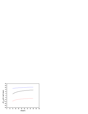
Figure 4: $g^{(B)}_{B_{s0}BK}(Q^{2}=1.0GeV^{2})$ as a function of the Borel mass $M^{2}$. The dot-dashed dashed and solid lines correspond to the perturbative, quark condensate and total contributions respectively.

Using $\Delta_{s}=\Delta_{u}=0.5\nobreak\,\mbox{GeV}$ for the continuum thresholds and fixing $Q^{2}=1\nobreak\,\mbox{GeV}^{2}$, we found a good stability of the sum rule for $g_{B_{s0}BK}^{(B)}$ for $M^{2}\geq 20\nobreak\,\mbox{GeV}^{2}$, as can be seen in Fig. 4.

Within this interval we need to choose the best value of the Borel mass to study the $Q^{2}$ dependence of the form factor. It is well known in QCDSR that for small values of the Borel variable, $M^{2}$, the sum rule is dominated by the pole. However, the convergence of the OPE always get better for large values of $M^{2}$. On the other hand, for very large values of $M^{2}$ the OPE convergence is perfect but the sum rule is dominated by the continuum. The best value of the Borel mass is the one for which one has a good OPE convergence and the pole contribution is bigger than the continuum contribution. In this case the both criteria are reasonably satisfied for $M^{2}\approx 35~{}\nobreak\,\mbox{GeV}^{2}\approx m^{2}_{B_{s}0}$.

In the case of $g_{B_{s0}BK}^{(K)}(Q^{2})$, doing a similar analysis described above, we also fix $M^{2}\approx 35~{}\nobreak\,\mbox{GeV}^{2}\approx m^{2}_{B_{s}0}$.

Having determined $M^{2}$ we show, in Fig. 5, the $Q^{2}$ dependence of the form factors. The squares correspond to the $g_{B_{s0}BK}^{(B)}(Q^{2})$ form factor in the interval where the sum rule is valid. The circles are the results of the sum rule for the $g_{B_{s0}BK}^{(K)}(Q^{2})$ form factor.

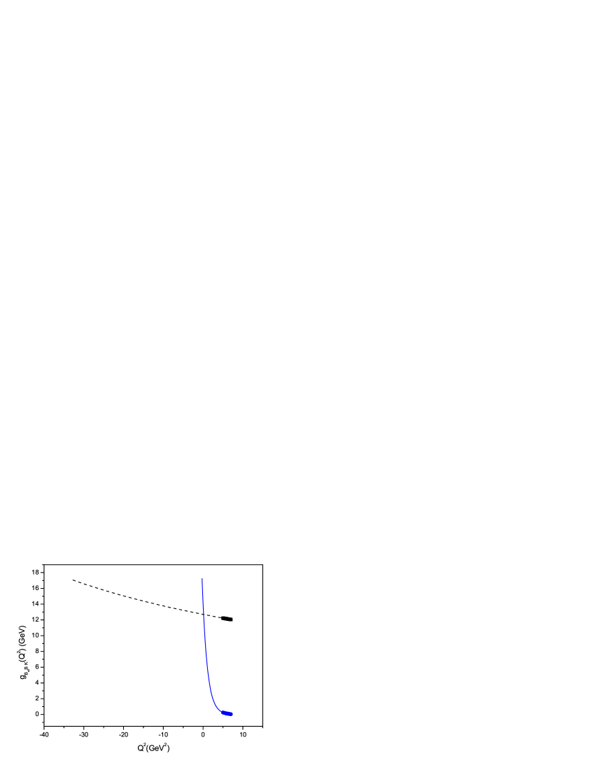
Figure 5: $g^{(B)}_{B_{s0}BK}$ (squares) and $g^{(K)}_{B_{s0}BK}$ (circles) QCDSR form factors as a function of $Q^{2}$. The dashed and solid lines correspond to the monopolar and exponetial parametrizations respectively.

In the case of an off-shell $B$ meson, our numerical results can be fitted by the following monopolar parametrization (shown by the dashed line in Fig. 5):

$$g_{B_{s0}BK}^{(B)}(Q^{2})=\frac{1,629.12\nobreak\,\mbox{GeV}^{3}}{Q^{2}+128.25\nobreak\,\mbox{GeV}^{2}}\;.$$ (37)

The coupling constant is defined as the value of the form factor at $Q^{2}=-m^{2}_{m}$, where $m_{m}$ is the mass of the off-shell meson. Therefore, using $Q^{2}=-m_{B}^{2}$ in Eq (37), the resulting coupling constant is:

$$g_{B_{s0}BK}=17.01~{}\nobreak\,\mbox{GeV}\;.$$ (38)

For an off-shell $K$ meson, our sum rule results can also be fitted by an exponential parametrization, which is represented by the solid line in Fig. 5:

$$g_{B_{s0}BK}^{(K)}(Q^{2})=14.14\nobreak\,\mbox{GeV}e^{-Q^{2}/1.25\nobreak\,\mbox{GeV}^{2}}\;.$$ (39)

Using $Q^{2}=-m_{K}^{2}$ in Eq (39) we get:

$$g_{B_{s0}BK}=17.23~{}\nobreak\,\mbox{GeV},$$ (40)

in a good agreement with the result of Eq.(38).

In order to study the dependence of our results with the continuum threshold, we vary $\Delta_{s,u}$ between $0.4\nobreak\,\mbox{GeV}\leq\Delta_{s,u}\leq 0.6\nobreak\,\mbox{GeV}$ in the parametrization corresponding to the case of an off-shell $K$. As can be seen in Fig. 6, this procedure gives us an uncertainty interval of $13.13\nobreak\,\mbox{GeV}\leq g_{B_{s0}BK}\leq 19.46\nobreak\,\mbox{GeV}$ for the coupling constant.

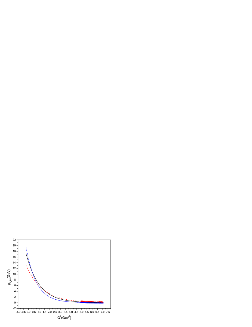
Figure 6: Dependence of the form factor on the continuum threshold for the $K$ off-shell case. The solid curve corresponds to $\Delta_{s,u}=0.5\nobreak\,\mbox{GeV}$, the dashed one to $\Delta_{s,u}=0.6\nobreak\,\mbox{GeV}$ and the dotted curve to $\Delta_{s,u}=0.4\nobreak\,\mbox{GeV}$.

We see that in the two cases considered here, off-shell $B$ or $K$, we get compatible results for the coupling constant, evaluated using the QCDSR approach. Considering the uncertainties in the continuum thresholds we obtain:

$$g_{B_{s0}BK}=(16.29\pm 3.16)~{}\nobreak\,\mbox{GeV}\;.$$ (41)

in a very good agreement with the coupling evaluated in ref. wang2 using light-cone QCDSR: $g_{B_{s0}BK}=(19.6\pm 5.7)~{}\nobreak\,\mbox{GeV}$.

In ref. gscpz the authors use a heavy-light chiral lagrangian and find the $B_{s0}$ to be a $BK$ bound state with the strong coupling $g_{B_{s0}BK}=23.442~{}\nobreak\,\mbox{GeV}$. This coupling is bigger than our result in Eq. (41), which is compatible with the expectation that a multiquark system would decay easily into its constituents.

The decay width for the decay $B_{s0}\to BK$ is given in terms of the coupling constant $g_{B_{s0}BK}$ through:

$$\Gamma(B_{s0}\to BK)={1\over 16\pi m_{B_{s0}}^{3}}g_{B_{s0}BK}^{2}\sqrt{\lambda(m_{B_{s0}}^{2},m_{B}^{2},m_{K}^{2})},$$ (42)

Considering the result in Eq. (41) and using two different values for $m_{B_{s0}}$, we give in Table 3 the predictions for the $B_{s0}\to BK$ decay width. We also include in this Table, the decay width obtained with the result from ref. gscpz .

$m_{B_{s0}}~{}(\nobreak\,\mbox{GeV})$	$\Gamma~{}(\nobreak\,\mbox{GeV})$ (this work)	$\Gamma~{}(\nobreak\,\mbox{GeV})$ (ref. gscpz )
5.775	$10\pm 4$	20
5.8	$50\pm 15$	100

Table 3: The $B_{s0}\to BK$ decay width.

IV Conclusions

We have used the QCDSR to study the two-point function for the $B_{s0}$ scalar meson, considered as a tetraquark state in a diquark-antidiquark configuration. The mass obtained for the $(bq)(\bar{q}\bar{s})$ scalar state: $m_{B_{s0}}=(5.85\pm 0.13)~{}\nobreak\,\mbox{GeV}$, is in agreement with other predictions using different structures. Therefore, if the $B_{s0}$ scalar meson is observed with a mass around 5.7 – 5.8 GeV, only this information will not be enough to discriminate its structure. However, the width of the state can also be used to help in this task. For this purpose we have also considered the QCDSR three-point function for the vertex $B_{s0}BK$ to evaluated the $B_{s0}BK$ coupling constant, considering the $B_{s0}$ scalar meson to be a normal $b\bar{s}$ state. With this configuration we find the coupling constant at the $B_{s0}BK$ vertex to be $g_{B_{s0}BK}=(16.29\pm 3.16)~{}\nobreak\,\mbox{GeV}$, in a very good agreement with calculation using light-cone QCDSR.

In Table 3 we have presented the predictions for the $B_{s0}\to BK$ decay width, using two different values for $m_{B_{s0}}$, and the couplings obtained considering the $B_{s0}$ as a $b\bar{s}$ state and a $BK$ bound state. As expected the width obtained in the case that $B_{s0}$ state is a multiquark state is much bigger than the width obtained for a $b\bar{s}$ state with the same mass. Therefore, with the knowledge of the decay width and the mass of the $B_{s0}$ it will be possible to discriminate between possible structures for this state.

- (1) T. Aaltonen et al., CDF Coll., Phys. Rev. Lett. 100, 082001 (2008) [arXiv:0710.4199].
- (2) V.M. Abazov et al., D0 Coll., Phys. Rev. Lett. 100, 082002 (2008) [arXiv:0711.0319].
- (3) F.-K. Guo et al., Phys. Lett. B 641, 278 (2006) [hep-ph/0603072].
- (4) Z.-G. Wang, Commun. Theor. Phys. 52, 91 (2009) [arXiv:0712.0118].
- (5) J. Vijande, A. Valcarce, F. Fernandez, Phys. Rev. D 77, 017501 (2008).
- (6) Z.-G. Wang, Phys. Rev. D 77, 054024 (2008) [arXiv:0801.0267].
- (7) A. Faessler et al., Phys. Rev. D 77, 054024 (2008) [arXiv:0801.2232].
- (8) M.A. Shifman, A.I. and Vainshtein and V.I. Zakharov, Nucl. Phys. B147, 385 (1979).
- (9) L.J. Reinders, H. Rubinstein and S. Yazaki, Phys. Rept. 127, 1 (1985).
- (10) For a review and references to original works, see e.g., S. Narison, QCD as a theory of hadrons, Cambridge Monogr. Part. Phys. Nucl. Phys. Cosmol. 17, 1 (2002) [hep-h/0205006]; QCD spectral sum rules , World Sci. Lect. Notes Phys. 26, 1 (1989); Acta Phys. Pol. B26, 687 (1995); Riv. Nuov. Cim. 10N2, 1 (1987); Phys. Rept. 84, 263 (1982).
- (11) M.E. Bracco et al., Phys. Lett. B624, 217 (2005).
- (12) T. Kojo, D. Jido, Phys. Rev. D78, 114005 (2008).
- (13) J. Sugiyama, T. Nakamura, N. Ishii, T. Nishikawa and M. Oka, Phys. Rev. D76, 114010 (2007).
- (14) R.D. Matheus, F.S. Navarra, M. Nielsen, C.M. Zanetti, Phys. Rev. D80, 056002 (2009).
- (15) M. Nielsen, F.S. Navarra, S.H. Lee, arXiv:0911.1958,
- (16) Bagan et al., Nucl. Phys. B254 (1985) 55; D.J. Broadhurst and S. Generalis, Phys. lett. B139 (1984) 85.
- (17) B. L. Ioffe, Nucl. Phys. B188, 317 (1981); B191, 591(E) (1981).
- (18) S. Narison, Nucl. Phys. Proc. Suppl. 86 (2000) 242 (hep-ph/9911454); S. Narison, hep-ph/0202200; S. Narison, hep-ph/0510108; S. Narison, Phys. lett. B341 (1994) 73; H.G. Dosch and S. Narison, Phys. lett. B417 (1998) 173; S. Narison, Phys. lett. B216 (1989) 191.
- (19) S. Narison, Phys. Lett. B466, 345 (1999).
- (20) S. Narison, Phys. Lett. B361, 121 (1995); S. Narison, Phys. Lett. B387, 162 (1996). S. Narison, Phys.Lett. B624 (2005) 223.
- (21) R.D. Matheus, F.S. Navarra, M. Nielsen and R.R. da Silva, Phys. Rev. D 76, 056005 (2007) [arXiv:0705.1357].
- (22) F.S. Navarra et al., Phys. Lett. B 489, 319 (2000).
- (23) F. S. Navarra, M. Nielsen, M. E. Bracco, Phys. Rev. D 65, 037502 (2002).
- (24) M. E. Bracco et al. Phys. Lett. B 521, 1 (2001).
- (25) R.D. Matheus, F.S. Navarra, M. Nielsen and R.R. da Silva, Phys. Lett. B 541, 265 (2002).
- (26) R. D. Matheus, F. S. Navarra, M. Nielsen and R. Rodrigues da Silva, Int. Jour. Mod. Phys. E 14, 555 (2005).
- (27) F. Carvalho, F. O. Durães, F. S. Navarra and M. Nielsen, Phys. Rev. C 72, 024902 (2005).
- (28) M. E. Bracco, M. Chiapparini, F. S. Navarra and M. Nielsen, Phys. Lett. B 605, 326 (2005).
- (29) M. E. Bracco et al. Phys. Lett. B 641, 286 (2006).
- (30) L. B. Holanda, R. S. Marques de Carvalho and A. Mihara, Phys. Lett. B 644, 232 (2007).
- (31) M.E. Bracco, M. Chiapparini, F.S. Navarra, M. Nielsen, Phys. Lett. B 659, 559 (2008).
- (32) L. W. Chen, C. M. Ko, W. Liu, M. Nielsen, Phys. Rev. C 76, 014906 (2007) [arXiv:0705.1697].