Phase diagram and spectral properties of a new exactly integrable spin one quantum chain

Abstract

The spectral properties and phase diagram of the exact integrable spin one quantum chain introduced by Alcaraz and Bariev are presented. The model has a $U(1)$ symmetry and its integrability is associated to an unknown R-matrix whose dependence on the spectral parameters is not of difference form. The associated Bethe ansatz equations, that fix the eigenspectra, are distinct from those associated to other known integrable spin models. The model has a free parameter $t_{p}$. We show that at the special point $t_{p}=1$ the model gets an extra $U(1)$ symmetry and reduces to the deformed $SU(3)$ Perk-Schultz model at a special value of its anisotropy $q=\exp(i2\pi/3)$ and in the presence of an external magnetic field. Our analysis is done either by solving the associated Bethe-ansatz equations or by direct diagonalization of the quantum Hamiltonian for small lattice sizes. The phase diagram is calculated by exploring the consequences of conformal invariance on the finite-size corrections of the Hamiltonian eigenspectrum. The model exhibits a critical phase ruled by $c=1$ conformal field theory separated from a massive phase by first-order phase transitions.

I Introduction

The anisotropic spin $1/2$ Heisenberg model, or XXZ quantum chain, and the 6-vertex model are considered as paradigm of exact integrability in statistical mechanics yang . In the XXZ quantum chain the $z$-component of the total magnetization is a good quantum number ($U(1)$ symmetry). Its simplest integrable generalizations that keeps the $U(1)$ symmetry are spin-1 quantum chains. Models on this class are the Fateev-Zamolodchikov model fateev , the Izergin-Korepin model izergin , the supersymmetric $OSP(1/2)$ model virchirko and the biquadratic model biquadratic . The integrability of these models is a consequence of the existence of a known associated R-matrix satisfying the Yang-Baxter equation. The associated R-matrix for these models are regular, i.e., depends only on the difference of the spectral parameters.

A new exact integrable spin-1 quantum chain was derived by using the coordinate Bethe ansatz AB1 , or a matrix product ansatz MPA . The derivation of the integrable model through these last approaches does not depend on the knowledge of the associated $R$ matrix. Distinct from the other integrable fateev -biquadratic and non integrable blume spin-1 models, whose physical properties are well studied, almost no physical information is known for this new quantum chain, besides its exact integrability. The unknown associated R-matrix is not regular AB1 since it does not satisfy the Reshetikihin criterion kulish . The Bethe ansatz equations (BAE) that fix the eigenenergies are also quite distinct from the corresponding equations of other spin-1 integrable quantum chains.

In this paper we are going to present an extensive analytical and numerical analysis of the eigenspectra properties of this new spin-1 quantum chain. Based on solutions of the associated BAE, whenever it is possible, and diagonalizations of the quantum Hamiltonian on small lattices ($L=2-24$) we are able to predict some of its critical properties.

The paper is organized as follows. In section 2 we present the model and the BAE that fix the eigenspectra. The model has a $U(1)$ symmetry and is exact integrable for any value of a free parameter $t_{p}$. We show, that for the special value $t_{p}=1$, the model is related to the deformed $SU(3)$ Perk-Schultz model with deformation parameter $q=\exp(i2\pi/3)$ perk in the presence of an external magnetic field. In section 3 we analyze the eigenspectra of the quantum chain in several regions with distinct values of the free parameter $t_{p}$. Based on conformal invariance predictions the critical properties of the model are calculated. Finally in section 4 we summarize our results and present our conclusions.

II The model

Instead of presenting the quantum Hamiltonian in terms of spin-1 $SU(2)$ matrices ($S^{x},S^{y},S^{z}$) it is more convenient to present it in terms of the $3\times 3$ Weyl matrices $E^{l,m}$ ($l,m=0,1,2$), with elements $E^{l,m})_{i,j}=\delta_{l,i}\delta_{m,j}$. At each lattice site $i$ we may have zero particle ($n_{i}=0$), one particle ($n_{i}=1$) or two particles ($n_{i}=2$) or equivalently $S_{i}^{z}=-1$, $S_{i}^{z}=0$ and $S_{i}^{z}=1$, respectively. The dynamics of these particles, in a periodic chain with $L$ sites, is described by the Hamiltonian

$$H(t_{p},h)=-\sum_{j=1}^{L}\sum_{\alpha,\beta,\gamma,\mu=0}^{2}\Gamma_{\gamma,\mu}^{\alpha,\beta}E_{j}^{\gamma,\alpha}E_{j+1}^{\mu,\beta}-h\sum_{j=1}^{L}\sum_{\alpha=1}^{2}\alpha E_{j}^{\alpha,\alpha}$$ (1)

where

$$\Gamma_{0,1}^{1,0}=\Gamma_{1,0}^{0,1}=\Gamma_{1,2}^{2,1}=\Gamma_{2,1}^{1,2}=-1,\quad\Gamma_{2,0}^{0,2}=\Gamma_{0,2}^{2,0}=-t_{p},$$

$$\Gamma_{0,2}^{1,1}=\Gamma_{1,1}^{0,2}=e^{-i\pi/3}\sqrt{t_{p}^{2}-1},\quad\Gamma_{2,0}^{1,1}=\Gamma_{1,1}^{2,0}=-e^{i\pi/3}\sqrt{t_{p}^{2}-1},$$ (2)

are the hopping parameters (off diagonal) and the static terms (diagonal) are given by

$$\Gamma_{0,0}^{0,0}=\Gamma_{2,2}^{2,2}=0,\quad\Gamma_{1,0}^{1,0}=\Gamma_{0,1}^{0,1}=\frac{1}{4t_{p}},$$ (3)

$$\Gamma_{1,1}^{1,1}=t_{p}+\frac{1}{2t_{p}},\quad\Gamma_{0,2}^{0,2}=\Gamma_{2,0}^{2,0}=-\frac{t_{p}}{2},$$

$$\Gamma_{1,2}^{1,2}=\frac{1}{4t_{p}}+i\frac{\sqrt{3}}{2}t_{p},\quad\Gamma_{2,1}^{2,1}=\frac{1}{4t_{p}}-i\frac{\sqrt{3}}{2}t_{p}.$$

The parameter $t_{p}$ is free and $h$ plays the role of a magnetic field in the $z$ direction ($z$-magnetic field) or a chemical potential controlling the magnetization or the number of particles in the ground state, respectively.

The Hamiltonian (1) is non hermitian. It is interesting to observe that its non hermiticity is not only due to the presence of complex matrix elements in the diagonal (see (3)) (as happens in the quantum deformed $SU_{q}(N)$ models) but also due to the presence of complex non diagonal elements (see (II)). The Hamiltonian (1) has a $U(1)$ symmetry due to its commutation with the total density $\rho$ of particles:

$$\rho=\frac{n}{L},\quad n=\sum_{j=1}^{L}n_{j},\quad n_{j}=S_{j}^{z}+1=\sum_{\alpha=1}^{2}\alpha E_{j}^{\alpha,\alpha}.$$ (4)

As a consequence its associated eigenvector space can be separated into disjoint sectors labeled by the the total number of particles $n$ (or density $\rho$) or equivalently by its magnetization.

The quantum chain (1) corresponds to one of the exactly integrable models introduced in AB1 . It is given by the choice $\epsilon=1$ in Eq. (15) of AB1 . As compared with the original presentation of the model, we also added a harmless $z$-magnetic field so that the ground state of (1) at $h=0$ has, for any value of $t_{p}$ total density $\rho=1$ or equivalently zero magnetization. The Hamiltonian (1) is exact integrable for arbitrary values of the parameter $t_{p}$ and magnetic field $h$.

At $t_{p}=1$ the non-diagonal couplings $\Gamma_{2,0}^{1,1}=\Gamma_{1,1}^{2,0}=\Gamma_{0,2}^{1,1}=\Gamma_{1,1}^{0,2}=0$ and the model has an additional $U(1)$ symmetry. The number of sites with single and double occupancy are now conserved separately. The parameter $t_{p}$ can be interpreted as an anisotropy parameter, being $t_{p}=1$ the isotropic point. At this isotropic point, apart from a contribution $i\frac{\sqrt{3}}{2}\sum_{i=1}^{L}(E_{i}^{0,0}-E_{i+1}^{0,0})$, that vanishes in the periodic chain, the Hamiltonian, with $h=0$, is given by

$$H(t_{p}=1,h=0)=H_{PS}(i\frac{2\pi}{3})-\frac{3}{2}\sum_{j=1}^{L}E_{j}^{1,1}+\frac{L}{2},$$ (5)

where

$$H_{PS}(\gamma)=\sum_{j=1}^{L}\sum_{\alpha=0}^{2}\left\{\cosh\gamma E_{i}^{\alpha,\alpha}E_{i+1}^{\alpha,\alpha}\right.$$

$$\left.+\sum_{\beta=\alpha+1}^{2}\left[\sinh\gamma(E_{i}^{\beta,\beta}E_{i+1}^{\alpha,\alpha}-E_{i}^{\alpha,\alpha}E_{i+1}^{\beta,\beta})+E_{i}^{\alpha,\beta}E_{i+1}^{\beta,\alpha}+E_{i}^{\beta,\alpha}E_{i+1}^{\alpha,\beta}\right]\right\}$$ (6)

is the deformed spin-1 $SU(3)$ Perk-Schultz model perk at the special value of the deformation parameter $q=e^{\gamma}$, $\gamma=i2\pi/3$. This model is also known as the anisotropic $SU(3)$ Sutherland model sut . It is important to stress that the related Perk-Schultz Hamiltonian is the ferromagnetic one (signal $+$) in the presence of a special magnetic field (value $h^{1}=3/2$, $h^{2}=0$) favoring single occupied sites. A simple calculation show us that the ground state for the related Perk-Schultz model happens in the sector with total density $\rho=1$. It corresponds to the trivial state $|11\cdots 1>$ where all the sites are single occupied. The model (1), for $t_{p}\neq 1$, can then be considered as the spin-1 anisotropic Perk-Schultz model at $q=e^{i2\pi/3}$ with an additional parameter that breaks partially its symmetry. For arbitrary values of $t_{p}$ the eigenenergies and momentum are given by AB1

$$E=-n(\frac{1}{2t_{p}}+h)+2\sum_{j=1}^{n}\cos k_{j},\quad P=\sum_{j=1}^{n}k_{j},$$ (7)

where $\{k_{j}=k(\lambda_{j});j=1,\ldots,n\}$ are the roots obtained from the BAE

$$e^{ik_{j}L}=-\prod_{l=1}^{n}\frac{\sinh(\lambda_{j}-\lambda_{l}-i2\pi/3)}{\sinh(\lambda_{j}-\lambda_{l}+i2\pi/3)},\quad j=1,\ldots,n,$$ (8)

with

$$e^{ik_{j}}=\frac{\sinh\lambda_{j}-i\sqrt{3t_{p}^{2}+(4t_{p}^{2}-1)\sinh^{2}\lambda_{j}}}{t_{p}(\sinh\lambda_{j}+i\sqrt{3}\cosh\lambda_{j})}.$$ (9)

As we see from (9) the left-hand side of the BAE (8) are quite distinct from the corresponding equations for other exact integrable quantum chains. In order to consider the bulk limit ($L\to\infty$) it is then necessary to study these equations for small lattice sizes. These studies, as we are going to see in the next section, will give us educated guesses for the topology of the roots $\{\lambda_{j}\}$ related to the low lying eigenvalues.

Before closing this section it is interesting to consider the BAE (8)-(9) at $t_{p}=1$. In this case they are given by

$$\left[\frac{\sinh(\lambda_{j}-i\pi/3)}{\sinh(\lambda_{j}+i\pi/3)}\right]^{L}=-\prod_{l=1}^{n}\frac{\sinh(\lambda_{j}-\lambda_{l}-i2\pi/3)}{\sinh(\lambda_{j}-\lambda_{l}+i2\pi/3)},\quad j=1,\ldots,n.$$ (10)

These equations coincide with the BAE of the XXZ chain yang at the special value of its anisotropy $\Delta=-(q+1/q)=1/2$ ($q=e^{i2\pi/3}$). However, in the XXZ chain the density of particles is restricted to $0\leq\rho\leq 1$ while in the model (1) $0\leq\rho\leq 2$. Although the completeness of the Bethe ansatz solutions is always a complicated problem, we expect that at $t_{p}=1$ the solution obtained from (10) is not complete. Due to the additional symmetry (conservation of the number of pairs of particles) we should start again the Bethe ansatz AB1 or the matrix product ansatz MPA taking into account this new symmetry. In this case we obtain the nested BAE of the deformed $SU(3)$ Perk-Schultz model with the deformation parameter value $q=e^{i2\pi/3}$. At this point this last model is special. In alcastro several conjectures about the eigenspectra of this model on its antiferromagnetic regime was done. As is well known the eigenspectra of the anisotropic $SU(3)$ Perk-Schultz model contains all the eigenvalues of the XXZ quantum chain with the same anisotropy. The equivalence (5) then indicates that the whole eigenspectra of the XXZ with anisotropy $\Delta=1/2$ is contained in the eigenspectra of the Hamiltonian (1) at $t_{p}=1$. Moreover, a direct diagonalization of (1), with $t_{p}=1$ and $h=0$, shows that for small even lattice sizes ($L\leq 12$) the low lying eigenvectors, for densities $\rho<1$, coincide with those of the XXZ chain at the anisotropy $\Delta=1/2$. This means that there is no double occupancy of particles on these eigenstates. This can be understood from (5) due to the presence of the magnetic field favoring single occupied sites.

III Eigenspectra calculations

In this paper we restrict ourselves to the cases where the parameter $t_{p}$ is real and positive. The eigenvalues of $H(t_{p},h)$ are the same as those of $-H(-t_{p},-h)$. The Hamiltonian (1) although having a real trace is non hermitian. The exact eigenspectra calculations for lattice sizes $L\leq 12$ show that most of the eigenenergies are real. All the low lying eigenvalues being real numbers. Imaginary eigenvalues, appearing in complex-conjugates pairs, happen only for high excited states in the eigenspectrum. We also verify that when $h=0$ the ground state of (1) belongs, for general values of $t_{p}$, to the sector with density $\rho=1$. Moreover, for $h=0$, the low lying excited states in the sectors with densities $\rho=1+\frac{m}{L}$ and $\rho=1-\frac{m}{L}$ ($m=1,2,\ldots$) are degenerated. This degeneracy is not valid for higher excited states since the model (1) at $h=0$ does not have the symmetry under the conjugation of particles: $0\leftrightarrow 2$, $1\leftrightarrow 1$.

At $t_{p}=1$, where the model (1) recovers the deformed $SU_{q}(3)$ Perk-Schultz model at $q=e^{i2\pi/3}$ (see (II)) the model is massive (non zero gap). Our numerical results indicate the same massive behaviour for all values of $t_{p}\geq 0$ as long as $h=0$. As $h$ decreases (negative values) it reaches the critical field $h_{c}(t_{p})$. For $h\leq h_{c}(t_{p})$ the ground state changes continuously its density of particles $\rho=\rho(h)<1$. We do expect, in the plane ($t_{p},\rho$) a phase diagram with massless (critical) behaviour for $\rho<1$. In this critical regime the long-distance fluctuations should be ruled by a underlying conformal invariant field theory. The conformal central charge $c$ of the continuum theory can be estimated from the finite-size corrections of the ground-state energy $E_{0}(L,t_{p},\rho)$ of the finite-size $L$ chain cardy-affleck , i. e.,

$$\frac{E_{0}(L,t_{p},\rho)}{L}=e_{\infty}-\frac{\pi v_{s}c}{L^{2}}+o(L^{-2}),$$ (11)

where $e_{\infty}$ is the bulk limit of the ground-state energy per site and $v_{s}=v_{s}(t_{p},\rho)$ is the sound velocity that can be inferred from the energy-momentum dispersion relations. Moreover, for each primary operator $\Phi_{\Delta,\bar{\Delta}}$, with dimension $x_{\Phi}=\Delta+\bar{\Delta}$ and spin $s_{\Phi}=\Delta-\bar{\Delta}$ in the operator algebra of the underlying conformal theory, there exists an infinite tower of eigenstates, whose energies $E_{m,m^{\prime}}^{\Phi}(L)$ and momentum $P_{m,m^{\prime}}^{\Phi}$ behave asymptotically as cardy

$$E_{m,m^{\prime}}^{\Phi}(L)=E_{0}(L)+\frac{2\pi}{L}v_{s}(x_{\Phi}+m+m^{\prime})+o(L^{-1}),$$

$$P_{m,m^{\prime}}^{\Phi}=\frac{2\pi}{L}(s_{\Phi}+m-m^{\prime}),$$ (12)

with $m,m^{\prime}=0,1,2,\ldots$.

Our spectral analysis of the Hamiltonian (1) was done by solving numerically the BAE (8)-(9) using a Newton type method, whenever it was possible. Since there is no numerical method that warranties the solution for the non linear equation (8), the success in finding the solutions depends very much on the ability to provide educated guesses for the approximated values. In the cases where we were not able to obtain the solutions of the BAE our analysis were based on direct numerical diagonalizations, or by using approximated methods like the power method. On these last cases our analysis were limited for lattice sizes up to $L=24$ sites.

According to the different topologies of roots of the BAE (8)-(9) we divide the plane ($t_{p},\rho$) in five regions (see Fig. 1).

Figure 1: Phase diagram of the quantum Hamiltonian (1)-(3). In regions 1 and 2 the ground state is described by real roots of the BAE. In the other regions the ground state, besides real roots, also contains complex ones. Regions 1,2,3 and 5 are critical and governed by $c=1$ Coulomb gas conformal field theory. Region 4 is characterized by several crossing of the eigenenergies producing an oscillatory behaviour in the finite energy gaps and momentum. The lines separating regions 1 and 5, and regions 2 and 3 are obtained by solving (19)-(21) and (23). An schematic line (heavy line) where we expect a first-order phase transition, separating region 3 and 4, is also shown.

In general the roots $\{\lambda_{j}\}$ of (8) are complex numbers. Numerical analysis, based on direct solutions of (8), as compared with brute force diagonalizations of the quantum chains shows that in regions 1 and 2 (see Fig 1) the roots $\{\lambda_{j}\}$ corresponding to the low lying eigenvalues are all real numbers. For these cases, the right-hand side of (8) is unimodular. The roots are then constrained or not on an finite real interval, depending on the values of $t_{p}$. If $t_{p}<1/2$ (region 1) the real roots are constrained on the interval

$$-\Omega(t_{p})<\lambda_{j}<\Omega(t_{p}),$$ (13)

where

$$\Omega(t_{p})=\frac{1}{2}\cosh^{-1}(\frac{2t_{p}^{2}+1}{1-4t_{p}^{2}}).$$ (14)

For $t_{p}\geq 1/2$ (region 2) these roots are unconstrained. For these real roots the BAE (8)-(9) take the simple from

$$Lk(\lambda_{j})=2\pi Q_{j}^{(n)}+\sum_{k=1}^{n}\phi(\lambda_{j},-\lambda_{k}),\quad j=1,\ldots,n,$$ (15)

where

$$k(\lambda)=\theta_{2}(\lambda)-\theta_{1}(\lambda),\quad\phi(\lambda)=2\arctan(\frac{\tanh\lambda}{\sqrt{3}}),$$

$$\theta_{2}(\lambda)=-\arctan(\frac{\sqrt{3t_{p}^{2}+(4t_{p}^{2}-1)\sinh^{2}\lambda}}{\sinh{\lambda}}),$$

$$\theta_{1}(\lambda)=\arctan(\sqrt{3}\coth\lambda),$$ (16)

and $Q_{j}^{(n)}$ ($j=1,\ldots,n$) are integers or odd-half integers, depending on the particular eigenstate. As before the eigenenergies and momenta are given by (7).

In order to illustrate we present in table 1 some eigenenergies obtained by solving the BAE (15) in region 1. We take in (1) the magnetic field $h=0$. They are obtained for several lattice sizes $L$ at $t_{p}=0.2$, $0.3$ and $0.4$ and densities $\rho=0.6$, $0.65$, and $0.7$, respectively.

$L\setminus(t_{p},\rho)$	(0.2,0.6)	(0.3,0.65)	(0.4,0.7)
10	-2.24745586	-	-1.70579604
100	-2.23726600	-1.86555023	-1.69990939
200	-2.23719021	-1.86548482	-1.69653825
1000	-2.23716569	-1.86547050	-1.69651539
Ext.	-2.23716439	-1.86546561	-1.69624038

Table 1: Lowest eigenenergies per site of the Hamiltonian (1) with $h=0$ for some values of $L$, $t_{p}$ and density of particles $\rho$. These points belong to region 1 (see Fig. 1). They are obtained by solving directly the BAE (15). They last line is the asymptotic value obtained from the solution of (19)-(22).

They are zero (mod. $\pi$) momentum eigenstates with roots $\{\lambda_{j}\}$ symmetrically distributed around the origin. The corresponding quantum numbers in (III) are $Q_{j}^{(n)}=\pm(-\frac{L}{2}+j)$ ($j=1,\ldots,n=\rho L$). The finite-size corrections of the ground state energies indicate us that in region 1 and 2 the Hamiltonian (1) is critical and conformally invariant. The relation (11) gives us an estimate for the conformal anomaly $c$ of the underlying conformal field theory. In Fig. 2 we show, as an example, the ground-state energy per site as a function of $1/L^{2}$, for the quantum chain with $t_{p}=0.2$, density $\rho=0.6$ and $h=0$. We clearly see a linear behaviour as predicted by conformal invariance (see (11)). The linear coefficient of the dot line in Fig. 2 gives us, from (11), an estimate

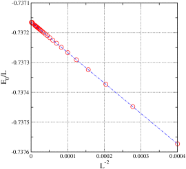
Figure 2: Ground state energy per site of the Hamiltonian (1) as a function of $1/L^{2}$, for $t_{p}=0.2$, $\rho=0.6$. We set $h=0$ in the figure. This point belongs to region 1 in Fig. 1.

for the product $2\pi v_{s}c$. The sound velocity $v_{s}$ is more difficult to estimate from numerical solutions of (15)-(III), since it demands the calculation of excited states with non zero momenta. The BAE roots on this case are not symmetric. A possible way to circumvent this problem is to seek for excited zero momentum states related to higher values of $m=m^{\prime}$ in the conformal tower (III) of the identity operator ($x_{\phi}=0$). Our numerical analysis indicate that these energies have a configuration of BAE roots where $\rho L-2$ of them are real and symmetrically distributed around the origin, and the two out-most roots are in the form $\lambda=\pm(a+i\pi)$, with $a\in\Re$. There is a difficulty in using this set of eigenlevels. As we change the lattice size their relative positions $m=m^{\prime}$ in the conformal tower are not fixed. However the estimates for the sound velocity obtained by direct diagonalization ($L\leq 24$) of the quantum chain, although with low precision, are enough to indicate the position $m=m^{\prime}$ of the eigenlevel in the conformal tower. Using this procedure we computed the conformal anomaly at several points in regions 1 and 2 (see Fig. 1) obtaining $c=1.00(1)$.

Since in regions 1 and 2 the ground state is described by real roots of the BAE, it is not difficult, in this case, to consider the bulk limit ($L\to\infty$) of the BAE (15)-(III). Following Baxter baxter we define the variables

$$x_{j}=\frac{Q_{j}}{L}=\frac{1}{2\pi}\left[k(\lambda_{j})-\frac{1}{L}\sum_{l=1}^{\rho L}\theta(\lambda_{j}-\lambda_{l})\right].$$ (17)

When $L\to\infty$, $x_{j}\to x$ become a continuous variable in the interval $x_{\mbox{\scriptsize min}}<x<x_{\mbox{\scriptsize max}}$ satisfying the integral equation

$$x_{j}=\frac{Q_{j}}{L}=\frac{1}{2\pi}\left[k(\lambda_{j})-\int_{x_{\mbox{\scriptsize min}}}^{x_{\mbox{\scriptsize max}}}\phi(\lambda(x)-\lambda(y))dy\right].$$ (18)

Since for the ground state the $\{Q_{j}\}$ are equally spaced by the unity, $\sigma_{L}(\lambda)=\frac{dx}{d\lambda}$ will give us, for $L\to\infty$, the local density of roots $\sigma_{\infty}(\lambda)$, that satisfies the integral equation

$$\sigma_{\infty}(\lambda)=\frac{1}{2\pi}\left(\frac{dk(\lambda)}{d{\lambda}}+\int_{-\lambda_{0}}^{\lambda_{0}}\frac{2\sqrt{3}\sigma_{\infty}(\lambda^{\prime})}{2\cosh(2(\lambda-\lambda^{\prime}))+1}d\lambda^{\prime}\right),$$ (19)

where from (III)

$$\frac{dk(\lambda)}{d\lambda}=\frac{\sqrt{3}}{2\cosh(2\lambda)+1}\left(1+\frac{\sqrt{3}\cosh\lambda}{\sqrt{(4t_{p}^{2}-1)\sinh^{2}\lambda+3t_{p}^{2}}}\right),$$ (20)

and $\lambda_{0}=\lambda_{0}(t_{p},\rho)$ gives the extreme values of the roots. The total density of particles and the ground-state energy per site are given by

$$\rho=\int_{-\lambda_{0}}^{\lambda_{0}}\sigma_{\infty}(\lambda)d\lambda,$$ (21)

$$\epsilon_{0}(t_{p},\rho,h)=\epsilon_{0}(t_{p},\rho,0)-h\rho=-\rho(\frac{1}{2t_{p}}+h)+2\int_{-\lambda_{0}}^{\lambda_{0}}\cos((k(\lambda))\sigma_{\infty}(\lambda)d\lambda,$$ (22)

where $h=h(t_{p},\rho)$ is the magnetic field that fixes the ground-state energy at the density $\rho$.

For $t_{p}<1/2$ (region 1), $\lambda_{0}(t_{p},\rho)$ is always finite, i. e., $\lambda_{0}(t_{p},\rho,h)\leq\Omega(t_{p})$ (see (14)). In Fig. 3 we show the ground-state energy $\epsilon_{0}(t_{p},\rho,h)$ for several values of $t_{p}$ in region 1 (we set $h=0$ in the figure).

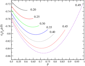
Figure 3: Ground state energy per site of the Hamiltonian (1) as a function of the density $\rho$, for several values of $t_{p}$ in region 1. In the figure we set $h=0$ and the values of $t_{p}$ are shown. These curves are obtained by solving (19)-(21). For a given value of $t_{p}$ the curves are shown for $\rho<\rho_{\mbox{\scriptsize max}}(t_{p})$, with $\rho_{\mbox{\scriptsize max}}(t_{p})$ given by (23). For $\rho>\rho_{\mbox{\scriptsize max}}(t_{p})$ there exist complex roots in the BAE solutions for the ground state and the model is in region 5.

They are obtained by using in (22) the $\sigma_{\infty}(\lambda)$ obtained from the numerical solution of the coupled integral equations (19)-(21). As we see from this figure these equations give us a maximum total density of particles $\rho=\rho_{\mbox{\scriptsize max}}(t_{p})<1$ for the quantum chain. At the endpoints of the curves we have $\lambda_{0}=\Omega(t_{p})$ (see (14)). Above this density, which we refer as region 5, some of the BAE roots associated to the ground state of the quantum chain have complex values. In Fig. 1 the line separating regions 1 and 5 gives, for a given $t_{p}$, the maximum density obtained from (19)-(21). This line was obtained by solving numerically (19)-(21). In order to compare with the finite-size results we give in the last line of table 1 the estimated value of $\epsilon_{0}(t_{p},\rho,h=0)$, obtained by solving (19)-(21) for $t_{p}=0.2,\;0.3$ and $0.4$ with $\rho=0.6,\;0.65$ and $0.7$, respectively.

For $t_{p}\geq 1/2$ (region 2) the roots $\{\lambda_{j}\}$ are not constrained and $\lambda_{0}=\lambda_{0}(t_{p},n)$ is arbitrary. The maximum density compatible with only real roots of the BAE for the ground state is obtained by setting $\lambda_{0}\to\infty$ in (19) and (21). In this case we can solve (19)-(21) by using Fourier transforms. After some long, but straightforward calculation we obtain the maximum density

$$\rho_{\mbox{\scriptsize max}}(t_{p})=\int_{0}^{\infty}\frac{3\sqrt{3}}{2\cosh(2\lambda)+1}\left(1+\frac{\sqrt{3}\lambda}{\sqrt{(4t_{p}^{2}-1)\sinh^{2}\lambda+3t_{p}^{2}}}\right)d\lambda.$$ (23)

At special values of $t_{p}$ we are able to solve (23) analytically: $\rho_{\mbox{\scriptsize max}}(1/2)=1$, $\rho_{\mbox{\scriptsize max}}(1)=1/2$, $\rho_{\mbox{\scriptsize max}}(\infty)=1/4$. In Fig. 1 the curve separating region 2 from 3 was obtained from the numerical evaluation of (23). As happened in region 5, for $\rho>\rho_{\mbox{\scriptsize max}}(t_{p})$ (regions 3 and 4), the BAE solutions giving the ground state contain complex roots besides the real ones.

As in region 1 (see table 1) we also calculated the finite-size corrections for the ground-state energy in several points of region 2. Using (11) and the same procedure as before our results indicate that, like region 1, region 2 is also critical and conformal invariant with $c=1$. We then have in both regions (1 and 2) a massless behaviour with ground-state energy given by real roots of the BAE. This critical behaviour is quite similar as that of the XXZ quantum chain in the presence of a magnetic field woyna ; xxz-h . We then expect in regions 1 and 2 a physical behaviour described by an underlying $c=1$ Coulomb gas conformal field theory. The anomalous dimensions of operators being given by

$$x_{l,m}=l^{2}x_{p}+m^{2}/4x_{p},$$ (24)

with $l,m=0,\pm 1,\pm 2,\ldots$. The dimensions $l^{2}x_{p}$ are obtained from (III), by considering the difference between the ground-state energies in the sectors with densities $\rho$ and $\rho+l/L$. The dimensions $x_{0,m}$ are calculated by using in (III) the mass gaps associated to eigenstates with the same density of particles.

The parameter $x_{p}=x_{p}(t_{p},\rho)$ in regions 1 and 2, which are estimated from the finite-size corrections of the energy (22), can be calculated analytically. This is done by applying to our relations (18)-(22) the method used in woyna for the XXZ quantum chain in a magnetic field. We obtain

$$x_{p}=(2\xi(\lambda_{0}))^{-2},$$ (25)

where $\xi(\lambda_{0})$ is the dressed charge korepin evaluated at the Fermi surface $\lambda_{0}$ of the effective Coulomb gas. This function satisfy the integral equation

$$\xi(\lambda)=1+\frac{\sqrt{3}}{\pi}\int_{-\lambda_{0}}^{\lambda_{0}}\frac{\xi(\lambda^{\prime})}{2\cosh(\lambda-\lambda^{\prime})+1}d\lambda^{\prime}.$$ (26)

In Fig. 4 we show, for several values of $t_{p}$ in regions 1 and 2, the dimensions $x_{p}=x_{p}(t_{p},\rho)$ obtained by using in (25) the numerical solutions of the coupled integral equations (19), (21) and (26). We can see from this figure that for any $t_{p}$, as $\rho\to 0$, $x_{p}\to 1/4$. This can be understood from the fact that at this limit the interacting potential energy is negligible when compared with the kinetic energy (hopping terms). We have essentially non-interacting particles, where $x_{p}$ has the value 1/4. We also see from this figure that, for $t_{p}<1/2$ (region 1), the limiting value of $x_{p}$ depends on the value of $t_{p}$. This value is obtained by choosing $\lambda_{0}=\Omega(t_{p})$ in (26), where $\Omega(t_{p})$ is given by (14). In Fig.  5 we show the limiting values of $x_{p}$ as a function of $t_{p}$, for $t_{p}\leq 1/2$.

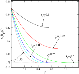
Figure 4: The values of $x_{p}(t_{p},\rho)$ (see (24)) as a function of $\rho$ for several values of $t_{p}$ in regions 1 and 2. The curves with $t_{p}<1/2$ and $t_{p}\geq 1/2$ belong to regions 1 and 2 of Fig. 1, respectively. The endpoints of the curves are the densities separating regions 1 and 2 from 3 and 5, respectively. For $t_{p}\geq 1/2$ the endpoints of the curves is $x_{p}=1/6\sim 0.16666$.

Figure 5: The values of $x_{p}$ at the line separating regions 1 and 5 (see Fig. 1). The exponents varies from $x_{p}=1/4$ to $x_{p}=1/6\sim 0.1666$, as $t_{p}$ goes from 0 to 1/2.

It varies from $x_{p}=1/4$ to $x_{p}=1/6$ as $t_{p}$ goes from 0 to 1/2. Moreover, Fig. 4 shows that the limiting value is $x_{p}=1/6$ for any $t_{p}\geq 1/2$. This should be the case since for any $t_{p}\geq 1/2$ the maximum value of $\lambda_{0}$ is infinity and consequently (25) and (26) give us the same result for any value of $t_{p}$. The exact value $x_{p}=1/6$ can be understood from the relation (see Sec. II) of the model at $t_{p}=1$ and the XXZ chain with anisotropy $\Delta=1/2$. When $\lambda_{0}\to\infty$ the density $\rho\to 1/2$. At this density the XXZ has no magnetic field and its exponent is given by $x_{p}=(\pi-\cos^{-1}(-\Delta))/2\pi=1/6$. These results imply that, at the line separating regions 1 and 5, $x_{p}$ varies continuously from 1/4 to 1/6 and, in the line separating regions 2 and 3, it remains fixed to the value 1/6.

In regions 3 and 5 of Fig. 1 some of the roots of the BAE corresponding to the ground state have complex values. In fact in some points of these regions we were able, for small lattice sizes, to solve the BAE for the ground-state energy. We verified that besides real roots we also have pairs of 2-strings (pair of roots of type $\lambda_{\pm}=a+ib$, with $a,b\in\Re$). The mixture of real and complex roots in the BAE (8) produces numerical instabilities turning the numerical solution of the BAE a quite difficult task. Due to this difficulty, instead of solving the BAE (8) we have used the power method to calculate the lower part of the eigenspectrum. On this case, due to computer limitations, even exploring the $U(1)$ and translation symmetries of the quantum chain we are restricted to lattice sizes up to $L=24$, where the largest sector we can calculate the lowest eigenenergy has dimension 5,136,935 ($L=24$, $n=13$). Since the calculations are done for a fixed density of particles $\rho$ the larger number of sites we can use, and consequently get a better precision for our estimates, is at the density $\rho=1/2$.

$t_{p}$	$e_{\infty}$	$v_{s}$	$h$	c	$x_{+1,0}$	$x_{-1,0}$	$x_{0,1}$	$1/4x_{0,1}$
0.75	-1.11947	1.4321	-1.5911	1.000	0.168	0.169	1.490	0.168
1.0	-1.04904	1.2991	-1.5000	0.999	0.167	0.167	1.500	0.167
1.15	-1.02211	1.2252	-1.4686	0.999	0.170	0.169	1.498	0.167
1.25	-1.00792	1.1771	-1.4540	1.001	0.169	0.167	1.490	0.168
1.35	-0.99597	1.1300	-1.4425	1.001	0.169	0.167	1.490	0.168
1.50	-0.9812	1.0596	-1.4295	1.01	0.169	0.167	1.48	0.168

Table 2: The quantities $e_{\infty},v_{s},c,x_{+1,0},x_{-1,0}$ and $x_{0,1}$ for the Hamiltonian (1) with density $\rho=1/2$ and some values of $t_{p}$. The first line ($t_{p}=0.75$) corresponds to a point inside region 2 and the second one ($t_{p}=1$) to a point at the line separating regions 2 and 3. The remaining lines correspond to points in region 3 (see Fig. 1).

In table 2 we present some of our estimated values of several quantities that characterizes the critical behaviour of the quantum chain (1) inside region 3 ($t_{p}=1.15$, $1.15,1.35$ and $1.5$). The calculations were done at density $\rho=1/2$. In the first two lines, for comparison, we also give the results for a point inside region 2 ($t_{p}=0.75$) and a point at the line separating regions 2 and 3 ($t_{p}=1$). We include in the table the estimated values for the ground-state energy per particle in the bulk limit $e_{\infty}$ (we set $h=0$ in (1)), the sound velocity $v_{s}$ and the magnetic field $h$ that fixes the ground state at density $\rho=1/2$.

The value of the exponent $x_{+1,0}=x_{-1,0}=x_{p}$ for $t_{p}=0.75$ and $t_{p}=1$ are known from the solutions of (19), (21) and (26), i. e., $x_{p}=0.16770$ ($t_{p}=0.75$) and $x_{p}=0.1666$ ($t_{p}=1$). The comparison of these last results with the first two lines of table 2 indicates that the errors are in the last digit. Like regions 1 and 2, region 3 is also massless with a conformal central charge $c=1$. The dimensions $x_{+1,0}$ and $x_{-1,0}$ in table 2 are associated to the sectors with densities $\rho=\frac{1}{2}+\frac{1}{L}$ and $\rho=\frac{1}{2}-\frac{1}{L}$, respectively. These dimensions in a standard Coulomb gas phase, like in region 1 and 2, are equal and correspond to the dimensions $x_{\pm 1,0}$ in (24). We also show in table 2 the dimension $x_{0,1}$ related to the first gap with zero (mod. $\pi$) momentum in the sector containing the ground state. The dimensions $x_{\pm 1,0}$, as shown in the table, is close to $1/4x_{0,1}$, in agreement with (24). The dimensions in the first two lines of table II ($t_{p}=0.75$ and $t_{p}=1$) although close are not equal, as we can also check in Fig 4. Table II also indicate that inside region 3 the conformal dimensions almost does not change as we change $t_{p}$. Since our results are valid only for the density $\rho=1/2$ we do not know if this small (or no) variation remains valid for other points inside region 3.

Once in region 3 of Fig. 1 by increasing the value of $t_{p}$, for a fixed density, we reach region 4. In this region several eigenlevels crossings happen in the finite lattice. In Fig. 6 we show for $L=10$ (left) and $L=16$ (right) these crossings. The crossings among eigenlevels with distinct momenta are visualized directly in the figure. The kinks in the curves are due to the level crossings with the same momentum.

As we cross from region 3 to region 4 the ground-state energy shows a discontinuity on its derivative due to a change of its relative position with an excited eigenstate. Unfortunately also in this region, due to numerical instabilities, it is quite difficult to solve directly the BAE (8). The direct diagonalization of the quantum chain, except at the density $\rho=1/2$, can only be done for quite few lattice sizes. Our estimate of the line separating regions 3 and 4, shown in Fig. 1, is then just schematic. This indicates a first order phase transition along the line separating these regions.

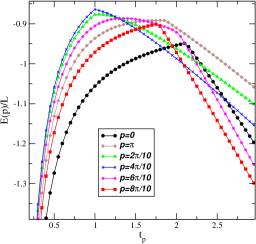
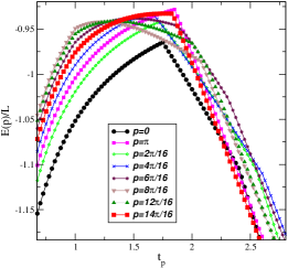
Figure 6: Lowest eigenenergy $E(p)$ with momentum $p$, as a function of $t_{p}$ for the Hamiltonian (1) at density $\rho=1/2$ and lattice sizes $L=10$ (left) and $L=16$ (right). We set $h=0$ in the figure. The energies $E(p)$ are the lowest eigenenergies with momentum $p$. The eigenlevels with $p\neq 0,\pi$ are doubled degenerated (momentum $p$ and $-p$). The kinks on the curves are due to a level crossing among the two lowest eigenenergies with the same momentum.

Inside region 4 and for $\rho=1/2$ we verify that the leading finite-size correction of the ground-state energy is not $O(1/L^{2})$ as expected in a massless conformaly invariant phase (see (11)). This is illustrated in Fig. 7 where we show for some values of $t_{p}$ the ground-state energy as a function of $1/L^{2}$ for the density $\rho=1/2$.

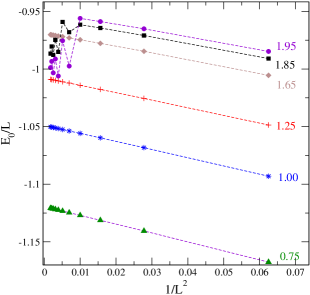
Figure 7: Ground state energy per particle as a function of $L^{-2}$ for the Hamiltonian (1) with $h=0$ at density $\rho=1/2$. The lattice sizes are $L=6,8,\ldots,24$. The curves correspond to $t_{p}=0.25,0.5$ (region 1), $t_{p}=0.75,1.00$ (region 2), $t_{p}=1.25$ (region 3) and $tp=1.85,1.95$ (region 4).

We see in this figure the distinct behaviour for the points belonging to regions 2 and 3 as compared with those of region 4 (lower two curves). The oscillatory behaviour in Fig. 7 for the points inside region 4 is a consequence of the level crossings happening inside this region. As we can see in Fig. 6 tor $t_{p}\sim 1.65$ many crossings happen with the crossing position dependent of the lattice size. As we change $t_{p}$ inside this region, for a given finite lattice $L$, the momentum of the ground state also changes. For example for $t_{p}\approx 2.25$ (see fig. 6) the ground state for the quantum chains with $L=10$ and $L=16$ has a non zero momentum and is doubled degenerated. The oscillatory behaviour shown in Fig. 7 turns out the finite-size scaling analysis quite imprecise. Although not conclusive these oscillatory behaviour in energy and momentum indicate that we have in region 4 effects of incommensurability of the density distributions, similar as happening in other models income .

In region 5, as in region 3, it is difficult to solve numerically the BAE due to the occurrence of complex roots mixed with real ones. In this case our analysis was restricted to small lattice sizes ($L\leq 24$). Since we should consider sequence of lattices with fixed density and on this region $\rho>1/2$, the number of data we can have on a given finite-size sequence is quite small. However, for a given lattice size and density, as we change $t_{p}$ we did not see the crossings of eigenlevels observed in region 4 (see figure 6). This indicates that region 5, similarly as regions 1,2 and 3 is a critical $c=1$ Coulomb gas phase. We greatly welcome more precise and convincing results for regions 4 and 5.

IV Summary and conclusions

We have made a detailed analysis of the spectral properties and phase diagram of the one of the new spin one model introduced in AB1 . This model is exact integrable for arbitrary values of the parameter $t_{p}$. Our analysis was restricted to the cases where $t_{p}>0$. At $t_{p}=1$ we have shown that the model recovers the deformed $SU(3)$ Perk-Schultz model (or spin-1 Sutherland model) at the special value of its deformation parameter $q=e^{i2\pi/3}$ and external magnetic field. We verified that at this point the low lying eigenvalues of the model are the same as the corresponding ones of the XXZ quantum chain with anisotropy $\Delta=1/2$. We can then interpret the model we studied as an integrable generalization of the deformed $SU(3)$ Perk-Schultz model or the XXZ quantum chain at anisotropy $\Delta=-(q+1/q)$ with $q=e^{i2\pi/3}$.

The BAE, whose solutions give the eigenspectrum of the model are quite difficult to solve analytically or numerically for general values of the parameter $t_{p}$ and density of particles (magnetization). Our results are summarized in Fig. 1, where we have regions 1-5.

Regions 1,2,3 and 5 belong to a critical phase governed by an underlying Coulomb gas conformal field theory with critical exponents varying continuously. We distinguished these regions according to the BAE roots of the low lying eigenenergies of the quantum chain. In regions 1 and 2 these roots are real. This fact allowed us to solve directly the BAE for quite large lattices ($L\sim 1000$). Exploring conformal invariance we obtain good estimates for the conformal anomaly and anomalous dimensions of operators of the underlying conformal field theory. In these two regions we could take the thermodynamic limit and obtained the critical exponents in terms of integral equations (see (25)-(26)).

In regions 3,4 and 5 the BAE roots corresponding to the ground state are not real and very difficult to calculate even for relatively small lattice sites. In these regions our analysis were based on the direct calculation of the eigenspectra for lattices sizes $L\leq 24$.

Our results indicated that, regions 3 and 5, although having BAE complex roots in the ground state, have the same critical behaviour as in regions 1 and 2. Actually regions 1,2,3 and 5 are quite similar to the XXZ quantum chain in the presence of a magnetic field, with anomalous dimensions $x_{l,m}$ given by (24), with the value of $x_{p}$ depending on $t_{p}$ and $\rho$.

As we cross from region 3 to region 4 there is a discontinuity of the ground-state energy. This is due to a crossing of the two lowest eigenenergies, and we expect that regions 3 and 4 are separated by a first order phase transition.

Inside region 4 we found an oscillatory behaviour for the energy gaps and momentum of the ground state, as we change the lattice size or the anisotropy parameter $t_{p}$. These oscillations are due to a large number of crossing of eigenlevels. These crossings made our finite-size analysis imprecise. We believe that probably such oscillatory behaviour is due to incommensurability effects on the charge (local magnetization) distribution in the lattice, as happens in other models whose incommensurability is established income .

We conclude mentioning two interesting open problems for the future. The derivation of the $R$-matrix associated to these new integrable spin one model and the extension of the present study to the second exact integrable model introduced in AB1 . This second model at $t_{p}=1$ is related to the XXZ quantum chain with anisotropy $\Delta=-1/2$. This last model has remarkable properties. It is related to the problem of enumerating alternated sign matrices alternating and the Hamiltonian with open boundaries is the evolution operator of a conformal invariant stochastic model, namely, the raise and peel model raise . We then expect that the second model in AB1 with values of $t_{p}\neq 1$ may also have interesting connections with other interesting problems in physics and combinatorics.

References

- (1) Yang C N and Yang C P 1966 Phys. Rev. 150 321; Yang C N and Yang C P 1966 Phys. Rev. 150 327
- (2) Zamolodchikov A B and Fateev V 1980 Sov. J. Nucl. Phys. 32 298; Babujian H 1982 Phys. Lett. 90A 479; Alcaraz F C and Martins M J 1988 Phys. Rev. Lett. 61 1529
- (3) Izergin A G and Korepin V E 1981 Commun. Math. Phys. 79 303
- (4) Virchirko V I and Reshetikhin N Yu 1983 Teor. Math. Phys. 56 805
- (5) Parkinson J B 1987 J. Phys. C: Solid State Phys. 20 L1029; Klümper A 1989 Europhys. Lett. 9 815; Batchelor M T, Mezincescu L, Nepomechie R I and Rittenberg V (1990) J. Phys. A: Math. Gen. 23 L141; Alcaraz F C and Malvezzi A L (1992) J. Phys. A: Math. Gen. 25 4535; Köberle R and Santos A L (1994) J. Phys. A: Math. Gen. 27 5409
- (6) Alcaraz F C and Bariev R Z 2001 J. Phys. A: Math. Gen. 34 l467
- (7) Alcaraz F C and Lazo M J 2004 J. Phys. A: Math. Gen. 37 L1; Alcaraz F C and Lazo M J 2004 J. Phys. A: Math. Gen. 37 4149
- (8) Blume M 1966 Phys. Rev. 141 517; Capel H W 1966 Physica (Amsterdam) 32 966; Alcaraz F C, Drugowich de Felício J R, Köberle R and Stilck J F 1985 Phys. Rev. B 32 7469; Haldane F D M 1983 Phys. Rev. Lett. 50 1153; Alcaraz F C and Hatsugai Y 1992 Phys. Rev. B 46 13914
- (9) Kulish P P and Sklyanin E K 1981 Lecture Notes on Physics 151 61
- (10) Perk J H H and Schultz C L 1981 Phys. Lett. A 84 407, Schultz C L 1983 Physica A 122 71
- (11) Sutherland B 1975 Phys. Rev. B 12 3795
- (12) Alcaraz F C and Stroganov Yu G 2002 J. Phys. A: Math. Gen. 35 3805; Alcaraz F C and Stoganov Yu G 2003 J. Phys. A: Math. Gen. 36 2381
- (13) Blöte H W J, Cardy J L and Nightingale M P 1986 Phys. Rev. Lett. 56, 742; Affleck I 1986 Phys. Rev. Lett. 56, 746
- (14) Cardy J L 1987 Phase Transitions and Critical Phenomena Vol.11, Eds. C Domb and J L Lebowitz (New York: Academic) p 55; Cardy J L 1986 Nucl. Phys. B 270 186
- (15) R.J. Baxter R J 1982 Exactly Solved Models in Statistical Mechanics (New York:Academic)
- (16) Woynarovich F, Eckle H P and Truong T T 1989 J. Phys. A: Math. Gen 22 4027
- (17) Jonhson J D and McCoy B M (1972) Phys. Rev. A 6 1613; Takanishi 1973 Prog. Theor. Phys. 50 1519; Alcaraz F C and Malvezzi A L (1995) J. Phys. A: Math. Gen. 28 1521
- (18) Korepin V E 1979 Teor. Math. Fiz. 41 169
- (19) Aligia A A, Batista C D and Essler F H L 2000 . Phys. Rev. B 62 3259; Hoeger C, von Gehlen G and Rittenberg V 1985 J. Phys. A: Math. Gen. 18 1813
- (20) Razumov A V and Stroganov Yu G 2001 J. Phys. A: Math. Gen. 34 3185; Batchelor M T, de Gier J and Nienhuis B 2001 J. Phys. A: Math. Gen. 34 L265; Razumov A V and Stroganov Yu G 2001 J. Phys. A: Math. Gen. 34 5335; de Gier J, Batchelor M T, Nienhuis B and Mitra S 2001 J. Math. Phys. 43 4235
- (21) de Gier J, Nienhuis B, Pearce P A and Rittenberg V (2204) J. Stat. Phys. 114 1; Alcaraz F C and Rittenberg V (2007) J. Stat. Mech. P08003