Simulating Nonholonomic Dynamics

Abstract.

This paper develops different discretization schemes for nonholonomic mechanical systems through a discrete geometric approach. The proposed methods are designed to account for the special geometric structure of the nonholonomic motion. Two different families of nonholonomic integrators are developed and examined numerically: the geometric nonholonomic integrator (GNI) and the reduced d’Alembert-Pontryagin integrator (RDP). As a result, the paper provides a general tool for engineering applications, i.e. for automatic derivation of numerically accurate and stable dynamics integration schemes applicable to a variety of robotic vehicle models.

1. Introduction

Nonholonomic constraints have been the subject of deep analysis since the dawn of Analytical Mechanics. Hertz, in 1894, was the first to use the term “nonholonomic system”, but we can even find older references in the work by Euler in 1734, who studied the dynamics of a rolling rigid body moving without slipping on a horizontal plane. Many authors have recently shown a new interest in that theory and also in its relation to the new developments in control theory, subriemannian geometry, robotics, etc (see, for instance, [24]). The main characteristic of this period is that Geometry was used in a systematic way (see L.D. Fadeev and A.M. Vershik [28] as an advanced and fundamental reference, and also, [1, 2, 5, 9, 18, 20] and references therein).

In the case of nonholonomic mechanics, these constraint functions are, roughly speaking, functions on the velocities that are not derivable from position constraints. Traditionally, the equations of motion for nonholonomic mechanics are derived from the Lagrange-d’Alembert principle which restricts the set of infinitesimal variations (or constrained forces) in terms of the constraint functions.

Recent works, such as [8, 10, 14, 23], have introduced numerical integrators for nonholonomic systems with very good energy behavior and properties such as the preservation of the discrete nonholonomic momentum map. In this paper, we will review and compare two new methods for nonholonomic mechanics, the Geometric Nonholonomic Integrator (GNI) [12] and the Reduced d’Alembert-Pontryagin Integrator (RDP) [17], examining their behavior in the numerical simulation of some of the most typical examples in nonholonomic mechanics: the Chaplygin sleigh and the snakeboard.

Finally, the developed algorithms are packaged as a general computational tool for automatic derivation of nonholonomic integrators given the system constraints and Lagrangian. It is available for download from
http://www.cds.caltech.edu/~marin/index.php?n=nhi

2. Introduction to Discrete Mechanics

Discrete variational integrators appear as a special kind of geometric integrators (see [13, 27]). These integrators have their roots in the optimal control literature in the 1960’s and 1970’s. In the sequel we will review the construction of this specific type of geometric integrators (see [22] for an excellent survey about this topic).

A discrete Lagrangian is a map $L_{d}\colon Q\times Q\rightarrow\mathbb{R}$, where $Q$ is a finite-dimensional configuration manifold. For the construction of numerical integrators for a continuous Lagrangian system given by a Lagrangian $L:TQ\rightarrow\mathbb{R}$, the discrete Lagrangian may be considered as an approximation of the integral action

$$L_{d}(q_{0},q_{1})\approxeq\int_{0}^{h}L(q(t),\dot{q}(t))\;dt$$

where $q(t)$ is a solution of the Euler-Lagrange equations corresponding to $L$, that is,

(1) $$\frac{d}{dt}\left(\frac{\partial L}{\partial\dot{q}}(q(t),\dot{q}(t))\right)-\frac{\partial L}{\partial{q}}(q(t),\dot{q}(t))=0\;,$$

additionally satisfying $q(0)=q_{0}$ and $q(h)=q_{1}$, where $h$ is the time step. Observe that this solution always exists if the Lagrangian is regular and $h$ is small enough (see [25]).

Define the action sum $S_{d}:Q^{N+1}\rightarrow\mathbb{R}$ corresponding to the Lagrangian $L_{d}$ by

$$S_{d}=\sum_{k=1}^{N}L_{d}(q_{k-1},q_{k}),$$

where $q_{k}\in Q$ for $0\leq k\leq N$. For any covector $\alpha\in T_{(x_{1},x_{2})}^{*}(Q\times Q)$, we have a decomposition $\alpha=\alpha_{1}+\alpha_{2}$ where $\alpha_{i}\in T^{*}_{x_{i}}Q$. Therefore,

$$dL_{d}(q_{0},q_{1})=D_{1}L_{d}(q_{0},q_{1})+D_{2}L_{d}(q_{0},q_{1})\;.$$

The discrete variational principle states that the solutions of the discrete system determined by $L_{d}$ must extremize the action sum given fixed points $q_{0}$ and $q_{N}$.

Extremizing ${S_{d}}$ over $q_{k}$, $1\leq k\leq N-1$, we obtain the following system of difference equations

(2) $$D_{1}L_{d}(q_{k},q_{k+1})+D_{2}L_{d}(q_{k-1},q_{k})=0\;.$$

These equations are usually called the discrete Euler-Lagrange equations.

The geometrical properties corresponding to this numerical method are obtained defining two discrete Legendre transformations associated to $L_{d}$ by

$$\begin{array}[]{rrcl}\mathbb{F}^{-}L_{d}:&Q\times Q&\longrightarrow&T^{*}Q\\ &(q_{0},q_{1})&\longmapsto&(q_{0},-D_{1}L_{d}(q_{0},q_{1}))\end{array}$$

$$\begin{array}[]{rrcl}\mathbb{F}^{+}L_{d}:&Q\times Q&\longrightarrow&T^{*}Q\\ &(q_{0},q_{1})&\longmapsto&(q_{0},D_{2}L_{d}(q_{0},q_{1}))\end{array}$$

and the 2-form $\omega_{d}=(\mathbb{F}^{\pm}L_{d})^{*}\omega_{Q}$, where $\omega_{Q}$ is the canonical symplectic form on $T^{*}Q$. We will say that the discrete Lagrangian is regular if $\mathbb{F}^{-}L_{d}$ is a local diffeomorphism. We will have that:

$$\mathbb{F}^{-}L_{d} \Leftrightarrow \mathbb{F}^{+}L_{d}$$ is a local diffeomorphism is a local diffeomorphism

$$\Leftrightarrow \omega_{d}$$ is symplectic

Under this regularity condition, this implicit system of difference equations (2) defines a local discrete flow $\Upsilon:U\subset Q\times Q\longrightarrow Q\times Q$, by $\Upsilon(q_{k-1},q_{k})=(q_{k},q_{k+1})$. The discrete algorithm determined by $\Upsilon$ preserves the symplectic form $\omega_{d}$, i.e., $\Upsilon^{*}\omega_{d}=\omega_{d}$. Moreover, if the discrete Lagrangian is invariant under the diagonal action of a Lie group $G$, then the discrete momentum map $J_{d}:Q\times Q\rightarrow{\mathfrak{g}}^{*}$ defined by $\langle J_{d}(q_{k},q_{k+1}),\xi\rangle=\langle D_{2}L_{d}(q_{k},q_{k+1}),\xi_{Q}(q_{k+1})\rangle$ is preserved by the discrete flow. Here, $\xi_{Q}$ denotes the fundamental vector field determined by $\xi\in{\mathfrak{g}}$:

$$\xi_{Q}(q)=\frac{d}{dt}\Big{|}_{t=0}(\hbox{exp}(t\xi)\cdot q)\;.$$

Therefore, these integrators are symplectic-momentum preserving integrators.

In [21] we have obtained a geometric derivation of variational integrators that is also valid for reduced systems (on Lie algebras, quotient of tangent bundles by a Lie group action, etc.)

3. Description of the nonholonomic dynamics

The presence of nonholonomic (or holonomic) constraints gives rise to forces. Nonholonomic systems are described by the Lagrange-D’Alembert’s principle which prescribes the constraint forces induced by the given nonholonomic constraints. In the following we will describe the equations of motion of a nonholonomic system in terms of Riemannian geometric tools (see [5]).

Let $Q$ be an $n$-dimensional differentiable manifold, with local coordinates $(q^{i})$, $1\leq i\leq n$. Consider a mechanical Lagrangian system $L:TQ\to\mathbb{R}$ defined by $L(v_{q})=\frac{1}{2}{\mathcal{G}}(v_{q},v_{q})-V(q)$, $v_{q}\in T_{q}Q$ or, locally

(3) $$L(q,\dot{q})=\frac{1}{2}g_{ij}(q)\dot{q}^{i}\dot{q}^{j}-V(q)\;.$$

Here ${\mathcal{G}}$ is a Riemannian metric on $Q$ (locally defined by the symmetric, positive definite matrix $(g_{ij}(q))_{1\leq i,j\leq n}$) and $V$ represents a potential function. We know that the equations of motion for a Lagrangian system are (1) which, in the case of a mechanical Lagrangian system of the form (3), admits a nice expression in terms of standard Riemmanian geometric tools:

$$\nabla_{\dot{c}(t)}\dot{c}(t)=-{\rm grad}~{}V(c(t))$$

where $\nabla$ is the Levi–Civita connection associated to ${\mathcal{G}}$ and, in coordinates, ${\rm grad}~{}V(c(t))=g^{ij}\frac{\partial V}{\partial q^{j}}$ where $(g^{ij})$ is the inverse matrix of $(g_{ij})$.

Assume that the system is subjected to nonholonomic constraints, defined by a regular distribution $\mathcal{D}$ on $Q$, with $\hbox{rank }\mathcal{D}=n-m$. Locally the nonholonomic constraints are described by the vanishing of $m$ independent functions

$$\phi^{a}=\mu^{a}_{i}(q)\dot{q}^{i},\quad 1\leq a\leq m\ \hbox{ (the ``constraint functions'')}.$$

The Lagrange–d’Alembert principle states that the equations of motion for a nonholonomic system determined by the two data $(L,\mathcal{D})$ are:

(4) $$\frac{d}{dt}\left(\frac{\partial L}{\partial\dot{q}^{i}}(q(t),\dot{q}(t))\right)-\frac{\partial L}{\partial{q}^{i}}(q(t),\dot{q}(t)) =\lambda_{a}\mu^{a}_{i}(q(t))\;,$$

$$\mu^{a}_{i}(q(t))\dot{q}^{i}(t) =0$$

where $\lambda_{a}$, $1\leq a\leq m$ are Lagrange multipliers to be determined. Using the Levi-Civita connection we find an intrinsic equation for the nonholonomic equations:

$$\nabla_{\dot{c}(t)}\dot{c}(t)=-{\rm grad}~{}V(c(t))+\bar{\lambda}(t),\quad\dot{c}(t)\in{\mathcal{D}}_{c(t)},$$

where $\bar{\lambda}$ is a section of ${\mathcal{D}}^{\perp}$ along $c$. Here ${\mathcal{D}}^{\perp}$ stands for the orthogonal complement of ${\mathcal{D}}$ with respect to the metric ${\mathcal{G}}$.

In coordinates, defining the $n^{3}$ functions $\Gamma^{k}_{ij}$ (Christoffel symbols for $\nabla$) by

$$\nabla_{\!\!\frac{\partial}{\partial q^{i}}}\,\frac{\partial}{\partial q^{j}}=\Gamma^{k}_{ij}\frac{\partial}{\partial q^{k}},$$

we may rewrite the nonholonomic equations of motion as

$$\ddot{q}^{k}(t)+\Gamma^{k}_{ij}(c(t))\dot{q}^{i}(t)\dot{q}^{j}(t) =-g^{ki}(c(t))\frac{\partial V}{\partial q^{i}}+\bar{\lambda}_{a}(t)g^{ki}(c(t))\mu^{a}_{i}(c(t))\;,$$

$$\mu^{a}_{i}(c(t))\dot{q}^{i}(t) =0\;.$$

4. Geometric Nonholonomic Integrator – GNI

Given a nonholonomic system $(L,\mathcal{D})$ where $L$ is a Lagrangian system of mechanical type (3), using the metric ${\mathcal{G}}$, we may consider the complementary projectors

$${\mathcal{P}}\colon TQ\rightarrow{\mathcal{D}}\hookrightarrow TQ$$

$${\mathcal{Q}}\colon TQ\rightarrow{\mathcal{D}}^{\perp}\hookrightarrow TQ$$

and their duals considered as mappings from $T^{*}Q$ to $T^{*}Q$.

The Geometric Nonholonomic integrator (GNI, in the sequel) for a nonholonomic system only needs to fix a discrete Lagrangian $L_{d}:Q\times Q\rightarrow\mathbb{R}$ to derive a numerical scheme, that is, it is not necessary to discretize the nonholonomic constraints for this type of integrator. The discrete nonholonomic equations proposed in [12] are

(5a) $${\mathcal{P}}^{*}_{|q_{k}}(D_{1}L_{d}(q_{k},q_{k+1}))+{\mathcal{P}}^{*}_{|q_{k}}(D_{2}L_{d}(q_{k-1},q_{k})) =0$$

(5b) $${\mathcal{Q}}^{*}_{|q_{k}}(D_{1}L_{d}(q_{k},q_{k+1}))-{\mathcal{Q}}^{*}_{|q_{k}}(D_{2}L_{d}(q_{k-1},q_{k})) =0.$$

The first equation is the projection of the discrete Euler–Lagrange equations to the dual of the constraint distribution $\mathcal{D}$, while the second one can be interpreted as an elastic impact of the system against $\mathcal{D}$. This defines a unique discrete evolution operator if and only if the Lagrangian $L_{d}$ is regular, in the sense of Section 2.

Define the pre- and post-momenta using the discrete Legendre transformations:

$$p^{+}_{k-1,k} =\mathbb{F}^{+}L_{d}(q_{k-1},q_{k})=(q_{k},D_{2}L_{d}(q_{k-1},q_{k}))\in T^{*}_{q_{k}}Q$$

$$p^{-}_{k,k+1} =\mathbb{F}^{-}L_{d}(q_{k},q_{k+1})=(q_{k},-D_{1}L_{d}(q_{k},q_{k+1}))\in T^{*}_{q_{k}}Q.$$

In these terms, equation (5b) can be rewritten as

$$\mathcal{Q}^{*}_{|q_{k}}\left(\frac{p^{-}_{k,k+1}+p^{+}_{k-1,k}}{2}\right)=0$$

which means that the average of post- and pre-momenta satisfies the nonholonomic constraints.

We can also rewrite the discrete nonholonomic equations as a jump of momenta:

(6) $$p^{-}_{k,k+1}=\left({\mathcal{P}}^{*}-{\mathcal{Q}}^{*}\right)\big{|}_{q_{k}}(p^{+}_{k-1,k}).$$

Reversibility.

Note that the map $\mathcal{S}=\mathcal{P}^{*}-\mathcal{Q}^{*}$ is an involution, that is $\mathcal{S}^{-1}=\mathcal{S}$. Therefore, it acts equivalently in both directions, i.e. it creates a reversible and symmetric flow. Furthermore, it can be expressed as

$$\mathcal{S}(q)=U(q)DU^{-1}(q),$$

where $D$ is a diagonal matrix with elements $\pm 1$ corresponding to the eigenvalues of $\mathcal{S}$ while $U$ is an invertible matrix with columns the eigenvectors of $S$. Thus, the update (6) can be written as

(7) $$U^{-1}(q_{k})p^{-}_{k,k+1}=DU^{-1}(q_{k})p^{+}_{k-1,k}$$

based on which one can regard the momentum as either remaining unchanged (corresponding to $+1$ eigenvalues) or being reflected (corresponding to $-1$ eigenvalues) with respect to the basis defined by the mapping $U^{-1}$.

Preservation Properties.

Suppose that $Q$ is a manifold on which a Lie group $G$ acts. Define for each $q\in Q$

(8) $$\mathfrak{g}^{q}=\left\{\xi\in\mathfrak{g}\,|\,\xi_{Q}(q)\in\mathcal{D}_{q}\right\},$$

where $\xi_{Q}(q)$ is the infinitesimal generator vector field corresponding to $\xi\in\mathfrak{g}$ at the point $q$. The bundle over $Q$ whose fiber at $q$ is $\mathfrak{g}^{q}$ is denoted by $\mathfrak{g}^{\mathcal{D}}$. Define the discrete nonholonomic momentum map $J^{\mathrm{nh}}_{d}\colon Q\times Q\to(\mathfrak{g}^{\mathcal{D}})^{*}$ as in [8] by

$$J^{\mathrm{nh}}_{d}(q_{k-1},q_{k})\colon\mathfrak{g}^{q_{k}} \to\mathbb{R}$$

$$\xi \mapsto\left\langle D_{2}L_{d}(q_{k-1},q_{k}),\xi_{Q}(q_{k})\right\rangle.$$

For any smooth section $\widetilde{\xi}$ of $\mathfrak{g}^{\mathcal{D}}$ we have a function $(J^{\mathrm{nh}}_{d})_{\widetilde{\xi}}\colon Q\times Q\to\mathbb{R}$, defined as $(J^{\mathrm{nh}}_{d})_{\widetilde{\xi}}(q_{k-1},q_{k})=J^{\mathrm{nh}}_{d}(q_{k-1},q_{k})\left(\widetilde{\xi}(q_{k})\right)$.

If $L_{d}$ is $G$-invariant and $\xi\in\mathfrak{g}$ is a horizontal symmetry (that is, $\xi_{Q}(q)\in\mathcal{D}_{q}$ for all $q\in Q$), then the GNI preserves $(J^{\mathrm{nh}}_{d})_{\xi}$ (see [12] for a proof).

In some cases of interest, it is possible to obtain an integrator preserving energy applying the following theorem (see [12]):

Theorem 1.

Let the configuration manifold be a Lie group with a bi-invariant Lagrangian and with an arbitrary distribution $\mathcal{D}$, and take a discrete Lagrangian that is left-invariant. Then the GNI (5) is energy-preserving.

4.1. Nonholonomic version of the RATTLE and SHAKE methods

Consider a continuous nonholonomic system determined by the mechanical Lagrangian $L\colon\mathbb{R}^{2n}\to\mathbb{R}$:

$$L({q},\dot{q})=\frac{1}{2}\dot{q}^{T}M\dot{q}-V(q)$$

(with $M$ a constant, invertible matrix) and the constraints determined by $\mu(q)\dot{q}=0$ where $\mu(q)$ is a $m\times n$ matrix with $\hbox{rank }\mu=m$.

Consider now the symmetric discretization

$$L_{d}(q_{k},q_{k+1}) =\frac{1}{2}hL\left(q_{k},\frac{q_{k+1}-q_{k}}{h}\right)+\frac{1}{2}hL\left(q_{k+1},\frac{q_{k+1}-q_{k}}{h}\right)$$

$$=\frac{1}{2h}\left(q_{k+1}-q_{k}\right)^{T}M\left(q_{k+1}-q_{k}\right)-\frac{h}{2}\left(V(q_{k})+V(q_{k+1})\right)\,.$$

After some straightforward computations we obtain that equations (5a) and (5a) for the proposed nonholonomic discrete system are

(9a) $$q_{k+1}-2q_{k}+q_{k-1} =-h^{2}M^{-1}\left(V_{q}(q_{k})+\mu^{T}(q_{k})\lambda_{k}\right)$$

(9b) $$0 =\mu(q_{k})\left(\frac{q_{k+1}-q_{k-1}}{2h}\right),$$

where $\lambda_{k}$ are Lagrange multipliers. We recognize this set of equations as an obvious extension of the SHAKE method proposed by [26] to the case of nonholonomic constraints.

The momentum is approximated by ${p}_{k}=M(q_{k+1}-q_{k-1})/2h$. Denoting $p_{k+1/2}=M(q_{k+1}-q_{k})/h$, equations (9a) and (9b) are now rewritten in the form

$$p_{k+1/2} ={p}_{k}-\frac{h}{2}\left(V_{q}(q_{k})+\mu^{T}(q_{k}){\lambda}_{k}\right),$$

$$q_{k+1} =q_{k}+hM^{-1}p_{k+1/2},$$

$$0 =\mu(q_{k})M^{-1}{p}_{k}.$$

The definition of ${p}_{k+1}$ requires the knowledge of $q_{k+2}$ and, therefore, it is is natural to apply another step of the algorithm (9a) and (9b) to avoid this difficulty. Then, we obtain the new equations:

$${p}_{k+1} ={p}_{k+1/2}-\frac{h}{2}\left(V_{q}(q_{k+1})+\mu^{T}(q_{k+1}){\lambda}_{k+1}\right),$$

$$0 =\mu(q_{k+1})M^{-1}{p}_{k+1}.$$

The interesting result is that we obtain a natural extension of the RATTLE algorithm for holonomic systems to the case of nonholonomic systems. Unifying the equations above we obtain the following numerical scheme

(10a) $$p_{k+1/2} ={p}_{k}-\textstyle\frac{h}{2}\left(V_{q}(q_{k})+\mu^{T}(q_{k})\lambda_{k}\right),$$

(10b) $$q_{k+1} =q_{k}+hM^{-1}p_{k+1/2},$$

(10c) $$0 =\mu(q_{k})M^{-1}{p}_{k},$$

(10d) $${p}_{k+1} ={p}_{k+1/2}-\textstyle\frac{h}{2}\left(V_{q}(q_{k+1})+\mu^{T}(q_{k+1})\lambda_{k+1}\right),$$

(10e) $$0 =\mu(q_{k+1})M^{-1}{p}_{k+1}.$$

These equations allow us to take a triple $(q_{k},p_{k},{\lambda}_{k})$ satisfying the constraint equations (10c), compute $p_{k+1/2}$ using (10a) and then $q_{k+1}$ using (10b). Then, equations (10d) and (10e) are used to compute the remaining components of the triple $(q_{k+1},p_{k+1},{\lambda}_{k+1})$. It is clear, applying Theorem 1 that, in the case $V=0$, the numerical method is energy preserving.

Remark 1.

From this Hamiltonian point of view, we have shown that the initial conditions for this numerical scheme are constrained in a natural way ($(q_{0},{p}_{0})$ with $\mu(q_{0})M^{-1}{p}_{0}=0$), that is, the initial conditions are exactly the same as those for the continuous system. Additionally, we select $\lambda_{0}=0$ (see [12]).

In [11], the following theorem is proven.

Theorem 2.

The nonholonomic RATTLE method is globally second-order convergent.

4.2. Projected Version of the Nonholonomic RATTLE

The proposed nonholonomic RATTLE method can be expressed without the use Lagrangian multipliers by projecting the equations of motion onto the constraint distribution through the projection $\mathcal{P}$ defined in §4.

Assuming that the Lagrangian is regular and that matrix $\mu$ is full rank (i.e. rank $m$) (9) can be reformulated as

(11a) $$\mathcal{P}(q_{k})^{T}M\left(q_{k+1}-2q_{k}+q_{k-1}\right) =-h^{2}\mathcal{P}(q_{k})^{T}V_{q}(q_{k})$$

(11b) $$\mathcal{Q}(q_{k})^{T}M\left(\frac{q_{k+1}-q_{k-1}}{2h}\right) =0,$$

where the $n\times n$ matrices $\mathcal{Q}$ and $\mathcal{P}$ represent both orthogonal projectors and have rank $m$ and $(n-m)$, respectively, and are defined by

(12a) $$\mathcal{Q}(q) =M^{-1}\mu(q)^{T}\left(\mu(q)M^{-1}\mu(q)^{T}\right)^{-1}\mu(q),$$

(12b) $$\mathcal{P}(q) =\operatorname{Id}-\mathcal{Q}(q),$$

where $\operatorname{Id}$ is the identity matrix.

Eqs. (11) correspond to (5) for the case $Q=\mathbb{R}^{n}$ and furthermore can be put in the “momentum jump” form by adding (11a) and (11b) to get

(13) $$q_{k+1} =q_{k}+\left(\operatorname{Id}-2M^{-1}\mathcal{Q}(q_{k})^{T}M\right)(q_{k}-q_{k-1})-h^{2}M^{-1}\mathcal{P}(q_{k})^{T}V_{q}(q_{k}).$$

For a more realistic example, we can add control inputs $u\in U\subset\mathbb{R}^{c}$ acting in the basis defined by the $(n\times c)$ matrix $B(q)$ to obtain the following discrete equations:

$$q_{k+1} =q_{k}+\left(\operatorname{Id}-2M^{-1}\mathcal{Q}(q_{k})^{T}M\right)(q_{k}-q_{k-1})+h^{2}M^{-1}\mathcal{P}(q_{k})^{T}f(q_{k},u_{k}),$$

where the forces $f:Q\times U\rightarrow T^{*}Q$ are given by $f(q,u)=B(q)u-V_{q}(q)$.

In terms of momentum variables the integrator can be equivalently expressed as

(14a) $$p_{k+1/2} =\left(\operatorname{Id}-2\mathcal{Q}(q_{k})^{T}\right)p_{k-1/2}+h\mathcal{P}(q_{k})^{T}f(q_{k},u_{k})$$

(14b) $$q_{k+1} =q_{k}+hM^{-1}p_{k+1/2}$$

providing an update scheme $(q_{k},p_{k-1/2})\Rightarrow(q_{k+1},p_{k+1/2})$.

A remaining critical step in completing the algorithm is to establish the link between the discrete variables $(q_{k},p_{k+1/2})$ for $k=0,...,N$ used in (14) and the continuous curve $(q(t),p(t))$. In that respect one can regard $p_{k}=(p_{k-1/2}+p_{k+1/2})/2$ as an approximation to the continuous momentum at time $t=kh$, i.e. $p_{k}\approx p(kh)$. The pair $(q_{k},p_{k})$ satisfies the nonholonomic constraint by definition and is related, following from (14), to the “midpoint” momenta through

(15a) $$p_{k} =\mathcal{P}(q_{k})^{T}p_{k+1/2}-\frac{h}{2}\mathcal{P}(q_{k})^{T}f(q_{k},u_{k}),$$

(15b) $$p_{k} =\mathcal{P}(q_{k})^{T}p_{k-1/2}+\frac{h}{2}\mathcal{P}(q_{k})^{T}f(q_{k},u_{k}).$$

These expressions can be used to determine proper variables $(q_{1},p_{1/2})$ to initialize the update (14) given continuous initial conditions $(q_{0},p_{0})\approx(q(0),p(0))$. Since there is a set of solutions $p_{1/2}$ satisfying (15) for a given $p_{0}$ the most natural choice is to pick $p_{1/2}$ satisfying the constraints at $q_{0}$. Therefore, the condition becomes

$$p_{1/2} =p_{0}+\frac{h}{2}\mathcal{P}(q_{0})^{T}f(q_{0},u_{0}).$$

In summary, given initial conditions $(q_{0},p_{0})$ satisfying the constraints, the dynamics is evolved forwards to reach the final state $(q_{N},p_{N})$, also in the constraint submanifold, after $N$ time steps through

(16) $$\begin{split}p_{1/2}&=p_{0}+\frac{h}{2}\mathcal{P}(q_{0})^{T}f(q_{0},u_{0}),\\ p_{k+1/2}&=\left(\operatorname{Id}-2\mathcal{Q}(q_{k})^{T}\right)p_{k-1/2}+h\mathcal{P}(q_{k})^{T}f(q_{k},u_{k}),\\ q_{k+1}&=q_{k}+hM^{-1}p_{k+1/2},\\ p_{N}&=\mathcal{P}(q_{N})^{T}p_{N-1/2}+\frac{h}{2}\mathcal{P}(q_{N})f(q_{N},u_{N}),\end{split}$$

for $k=1,...,N-1$.

5. Reduced d’Alembert-Pontryagin integrator-(RDP)

In this section we consider a class of mechanical systems which, in addition to nonholonomic constraints, also possess symmetries of motion arising from conservation laws. The interplay between the constraints and symmetries is linked to an intrinsic structure of the state space associated with important properties of the dynamics. Our goal in this section is to develop integrators that respect this structure and lead to more faithful numerical representation.

In §4 we introduced the action of a symmetry group $G$ and its relation the evolution of the system momentum. Additional structure arises whenever the dynamics and constraints are $G$-invariant that permits the construction of reduced nonholonomic integrators [14, 17].

Following [1], define the subspaces $\mathcal{V}_{q}$ and $\mathcal{S}_{q}$ according to

$$\mathcal{V}_{q}=\{\xi_{Q}(q)\ |\ \xi\in\mathfrak{g}\},\qquad\mathcal{S}_{q}=\mathcal{D}_{q}\cap\mathcal{V}_{q}.$$

Practically speaking, the vertical space $\mathcal{V}_{q}$ represents the space of tangent vectors parallel to symmetry directions while $\mathcal{S}_{q}$ is the space of symmetry directions that satisfy the constraints. Equivalently, $\mathcal{S}_{q}$ can be regarded as the space generated by elements in $\mathfrak{g}^{q}$, as defined in (8). The group $G$ is chosen so that the Lagrangian $L$ and distribution $\mathcal{D}$ are $G$-invariant. In addition, we make the standard assumption (see [1, 7]) that $T_{q}Q=\mathcal{D}_{q}+\mathcal{V}_{q}$, for each $q\in Q$.

Since our main interest is in a configuration space that is by construction of the form $Q=M\times G$ we will restrict any further derivations to the trivial bundle case. Using coordinates $(r,g)\in M\times G$ a basis for $\mathfrak{g}^{q}$ can be chosen as $\{e_{b}(r,g)\}$, for $b=1,...,\operatorname{dim}(\mathcal{S})$. Since $\mathcal{D}$ is $G$-invariant these elements can be expressed as $e_{b}(r,g)=\operatorname{Ad}_{g}e_{b}(r)$, where $\{e_{b}(r)\}$ is the body-fixed basis. We denote $\mathfrak{g}^{r}$ the space spanned by $\{e_{b}(r)\}$ at each $(r,e)\in Q$. Lastly, the system is subject to control force $f:[0,T]\rightarrow T^{*}M$ restricted to the shape space.

Nonholonomic Connection

With these definitions we can define a principal connection $\mathcal{A}:TQ\rightarrow\mathfrak{g}$ with horizontal distribution that coincides with $\mathcal{H}_{q}$ at the point $q$, where $\mathcal{D}_{q}=\mathcal{S}_{q}\oplus\mathcal{H}_{q}$. This connection is called the nonholonomic connection and is constructed according to $\mathcal{A}=\mathcal{A}^{\text{kin}}+\mathcal{A}^{\text{sym}}$, where $\mathcal{A}^{\text{kin}}$ is the kinematic connection enforcing the nonholonomic constraints and $\mathcal{A}^{\text{sym}}$ is the mechanical connection corresponding to symmetries satisfying the constraints. These maps are defined according to

(17) $$\begin{split}\mathcal{A}^{\text{kin}}(q)\cdot\dot{q}&=0,\\ \mathcal{A}^{\text{sym}}(q)\cdot\dot{q}&=\operatorname{Ad}_{g}\Omega,\end{split}$$

where $\Omega\in\mathfrak{g}^{r}$ is called the locked angular velocity, i.e. the velocity resulting from instantaneously locking the joints described by the variables $r$. Intuitively, when the joints stop moving the system continues its motion uniformly along a curve (with tangent vectors in $\mathcal{S}$) with body-fixed velocity $\Omega$ and a corresponding spatial momentum that is conserved.

By definition the principal connection can be expressed as

$$\mathcal{A}(q)\cdot\dot{q}=\operatorname{Ad}_{g}(g^{-1}\dot{g}+\mathcal{A}(r)\dot{r}),$$

where $\mathcal{A}(r)$ is the local form and the two components in (17) can be added to obtain

$$g^{-1}\dot{g}+\mathcal{A}(r)\dot{r}=\Omega.$$

Numerical Formulation

Since the Lagrangian is $G$-invariant, we can define the reduced Lagrangian $\ell:TM\times\mathfrak{g}\rightarrow\mathbb{R}$

(18) $$\ell(r,\dot{r},\xi)=L(r,\dot{r},e,g^{-1}\dot{g}).$$

In [17] a nonholonomic integrator was derived using a discrete variational d’Alembert-Pontryagin principle based on the reduced Lagrangian $\ell$, the connection $\mathcal{A}$ and a chosen trajectory discretization. In particular, a discrete trajectory with points $q_{k}=(r_{k},g_{k})\in M\times G$ and respective velocities $u_{k}\in TM$ and $\xi_{k}\in\mathfrak{g}$ was constructed so that

$$r_{k+1}-r_{k}=hu_{k},\qquad\tau^{-1}(g_{k}^{-1}g_{k+1})=h\xi_{k},$$

where $\xi_{k}=\Omega_{k}-\mathcal{A}(r_{k+\alpha})u_{k}$, with $r_{k+\alpha}:=(1-\alpha)r_{k}+\alpha r_{k+1}$ for a chosen $\alpha\in[0,1]$. The map $\tau:\mathfrak{g}\rightarrow G$ represents the difference between two configurations in the group by an element in its algebra and can be selected as:

• Exponential map $\exp:\mathfrak{g}\rightarrow G$, defined by $\exp(\xi)=\gamma(1)$, with $\gamma:\mathbb{R}\rightarrow G$ is the integral curve through the identity of the left invariant vector field associated with $\xi\in\mathfrak{g}$ (hence, with $\dot{\gamma}(0)=\xi$);

• Canonical coordinates of the second kind $\operatorname{ccsk}:\mathfrak{g}\rightarrow G$, $\operatorname{ccsk}(\xi)=\exp(\xi^{1}e_{1})\cdot\exp(\xi^{2}e_{2})\cdot...\cdot\exp(\xi^{n}e_{n})$, where $\{e_{i}\}$ is the Lie algebra basis.

A third choice for $\tau$, valid only for certain quadratic matrix groups [6] (which include the rigid motion groups $\operatorname{SO}(3)$, $\operatorname{SE}(2)$, and $\operatorname{SE}(3)$), is the Cayley map $\operatorname{cay}:\mathfrak{g}\rightarrow G$, $\operatorname{cay}(\xi)=(e-\xi/2)^{-1}(e+\xi/2).$ (See App. A for more details).

With these definitions in place the resulting reduced d’Alembert-Pontryagin (RDP) integrator can be stated [17]. For numerical convenience it is given in terms of vector-matrix notation, by treating the Lie algebra variables $\xi$ and $\Omega$ as vectors of coordinates with respect to a chosen canonical basis (see App. B for an example).

The discrete flow satisfies the reduced discrete dynamics

(27) $$\left[\begin{array}[]{cc}\operatorname{Id}&\left[\mathcal{A}(r_{k})\right]^{T}\\ {0}&[e_{1}(r_{k}),...,e_{c}(r_{k})]^{T}\end{array}\right]\left(\left[\begin{array}[]{c}\partial_{u}\ell_{k}\\ (\operatorname{d\tau}^{-1}_{h\xi_{k}})^{*}\partial_{\xi}\ell_{k}\end{array}\right]-\left[\begin{array}[]{c}\partial_{u}\ell_{k-1}\\ (\operatorname{d\tau}^{-1}_{-h\xi_{k-1}})^{*}\partial_{\xi}\ell_{k-1}\end{array}\right]\right)=\left[\begin{array}[]{c}hf_{k}\\ 0\end{array}\right],$$

where $\ell_{k}:=\ell(r_{k+\alpha},u_{k},\xi_{k})$ and $\xi_{k}=\Omega_{k}-\mathcal{A}(r_{k+\alpha})u_{k}$. The map $\operatorname{d\tau}_{\xi}:\mathfrak{g}\rightarrow\mathfrak{g}$ is the right-trivialized tangent of $\tau(\xi)$ defined by $\operatorname{D}\tau(\xi)\cdot\delta=TR_{\tau(\xi)}(\operatorname{d\tau}_{\xi}\cdot\delta)$ and $d\tau^{-1}_{\xi}:\mathfrak{g}\rightarrow\mathfrak{g}$ is its inverse (see App. A).

Equation (27) along with the reconstruction equations

(28) $$g_{k+1}=g_{k}\tau(h\xi_{k}),\qquad r_{k+1}=r_{k}+hu_{k},$$

constitute the complete RDP discrete evolution.

6. Examples

6.1. The Chaplygin Sleigh

The Chaplygin Sleigh [1] is a planar rigid body making a contact with the ground through a skate mounted at the central axis of the body at a distance $a$ from its center of mass (Fig. 1). The configuration space is the group $G=\operatorname{SE}(2)$ with coordinates $q=(\theta,x,y)$ describing the orientation and the position of the center of mass. The body has rotational inertia $I$ and mass $m$ and, therefore, its Lagrangian is defined by

(29) $$L(q,\dot{q})=\frac{1}{2}I\dot{\theta}^{2}+\frac{1}{2}m(\dot{x}^{2}+\dot{y}^{2}).$$

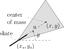
Figure 1. Chaplygin Sleigh model.

At the point of the skate contact $(x_{s},y_{s})=(x-a\cos\theta,y-a\sin\theta)$ the body must slide in the direction in which it is pointing. This condition is encoded by the nonholonomic constraint

$$a\dot{\theta}+\sin\theta\dot{x}-\cos\theta\dot{y}=0.$$

A structure-preserving integrator was developed in [10] based on the discrete Lagrange-d’Alembert (DLA) principle with discrete momentum and measure preservation properties. Exploring this direction further, in this section we develop two alternative methods based on the GNI and RDP schemes.

GNI Integrator.

From the mass matrix $M=\text{diag}(I,m,m)$ and the constraint $\mu_{1}(q)=[a,\sin\theta,-\cos\theta]$, the projector $\mathcal{Q}$ can be computed using (12a) as

(33) $$\mathcal{Q}(q)=\frac{1}{I+a^{2}m}\left[\begin{array}[]{ccc}a^{2}m&am\sin\theta&-am\cos\theta\\ aI\sin\theta&I\sin\theta^{2}&-I\sin\theta\cos\theta\\ -aI\cos\theta&-I\sin\theta\cos\theta&I\cos^{2}\theta\end{array}\right].$$

Since the mass matrix is constant, the GNI integrator can be derived according to $v_{k+\frac{1}{2}}=(\text{Id}-M^{-1}\mathcal{Q}(q_{k})^{T}M)v_{k-\frac{1}{2}}$. In terms of the coordinates $v=(v^{\theta},v^{x},v^{y})$, the discrete update becomes

$$\begin{split}&v_{k+\frac{1}{2}}^{\theta}=\left(1\!-\!\frac{2a^{2}m}{I^{\prime}}\right)v_{k-\frac{1}{2}}^{\theta}+\frac{am}{I^{\prime}}\left(-2\sin\theta_{k}v^{x}_{k-\frac{1}{2}}+2\cos\theta_{k}v^{y}_{k-\frac{1}{2}}\right),\\ &v_{k+\frac{1}{2}}^{x}=-\frac{2aI}{I^{\prime}}\sin\theta_{k}v_{k-\frac{1}{2}}^{\theta}+\left(1\!-\!\frac{2I}{I^{\prime}}\sin^{2}\!\theta_{k}\right)v_{k-\frac{1}{2}}^{x}+\frac{2I}{I^{\prime}}\sin\theta_{k}\cos\theta_{k}v_{k-\frac{1}{2}}^{y},\\ &v_{k+\frac{1}{2}}^{y}=\frac{2aI}{I^{\prime}}\cos\theta_{k}v_{k-\frac{1}{2}}^{\theta}+\frac{2I}{I^{\prime}}\sin\theta_{k}\cos\theta_{k}v_{k-\frac{1}{2}}^{x}+\left(1\!-\!\frac{2I}{I^{\prime}}\cos^{2}\theta_{k}\right)v_{k-\frac{1}{2}}^{y},\end{split}$$

where $I^{\prime}=I+a^{2}m$. It is straightforward to verify that the resulting update rule is energy-preserving, i.e. $\langle Mv_{k-1/2},v_{k-1/2}\rangle=\langle Mv_{k+1/2},v_{k+1/2}\rangle$. This property is inherent to the GNI construction as explained in [12].

RDP Integrator.

The sleigh has no internal joints and therefore no shape space. Since the Lagrangian (29) is left-invariant to $\operatorname{SE}(2)$ group action, the reduced Lagrangian (18) can be expressed as

$$\ell(\xi)=L(e,g^{-1}\dot{g}),$$

where $\xi=(\omega,v,v^{\perp})\in\mathfrak{g}$ describes the angular, forward, and sideways velocities with respect to the body frame fixed at the center of mass. The constrained symmetry space (8) of the sleigh can be identified as

$$\mathfrak{g}^{q}=\text{span}\{e_{1}(g),e_{2}(g)\},$$

where $e_{1}=(1,0,a)\in\mathfrak{g}$ and $e_{2}=(0,1,0)\in\mathfrak{g}$ form the constant basis in the body-fixed frame with $e_{i}(g)=\text{Ad}_{g}e_{i}$, for $i=1,2$. The two components of the nonholonomic momentum $p_{i}=\langle\partial_{\xi}\ell,e_{1}\rangle$ become

$$p_{1}=(J+a^{2}m)\omega,\qquad p_{2}=mv,$$

corresponding to angular and forward momenta, respectively. The group trajectory can be reconstructed from the momentum according to

$$g^{-1}\dot{g}=\left(\frac{1}{I+a^{2}m}p_{1},\ \frac{1}{m}p_{2},\ \frac{a}{I+a^{2}m}p_{1}\right).$$

The momentum components themselves evolve according to $\dot{p}_{i}=\langle\text{ad}^{*}_{\xi}\partial_{\xi}\ell,e_{i}\rangle$ (see  [2]), or equivalently

$$\dot{p}_{1}=-\frac{a}{I+a^{2}m}p_{1}p_{2},\qquad\dot{p}_{2}=\frac{ma}{(I+a^{2}m)^{2}}p_{1}^{2}.$$

Since the shape space consists of a single point, the discrete dynamics includes only the momentum equations (27) which become

$$\langle(\operatorname{d\tau}^{-1}_{h\xi_{k}})^{*}\partial_{\xi}\ell_{k}-(\operatorname{d\tau}^{-1}_{-h\xi_{k-1}})^{*}\partial_{\xi}\ell_{k-1},e_{i}\rangle=0,$$

for $i=1,2$. A simple form of these equations can be derived by choosing $\tau=\exp$ and truncating its tangent to first order, i.e. $\operatorname{d\tau}^{-1}_{\xi}\approx\text{Id}-\frac{1}{2}\text{ad}_{\xi}$. Using the notation $p_{k}=((p_{1})_{k},(p_{2})_{k})$ the update becomes

$$(p_{1})_{k}-(p_{1})_{k-1}=-\frac{ha}{2(J+a^{2}m)}\left[(p_{1})_{k}(p_{2})_{k}+(p_{1})_{k-1}(p_{2})_{k-1}\right],$$

$$(p_{2})_{k}-(p_{2})_{k-1}=\frac{hma}{2(J+a^{2}m)^{2}}\left[{(p_{1})_{k}}^{2}+{(p_{1})_{k-1}}^{2}\right].\vspace{-5pt}$$

These conditions are used to solve for the unknown next momentum $p_{k}$, e.g. through cubic equation root-finding. Note, that this particular choice of approximation exactly matches a standard implicit central difference discretization of the continuous ODE. This is generally not case for systems with non-constant Lie algebra basis element $e_{i}$ such as the snakeboard. Higher accuracy can be achieved through other choices of $\tau$ and better approximation of $\operatorname{d\tau}$. App. B details the cases $\tau=\exp$ and $\tau=\operatorname{cay}$ on $\operatorname{SE}(2)$.

The reconstruction equations are

$$g_{k+1}=g_{k}\exp(h\xi_{k}),$$

where

$$\xi_{k}=\left(\frac{1}{I+a^{2}m}(p_{1})_{k},\ \frac{1}{m}(p_{2})_{k},\ \frac{a}{I+a^{2}m}(p_{1})_{k}\right).$$

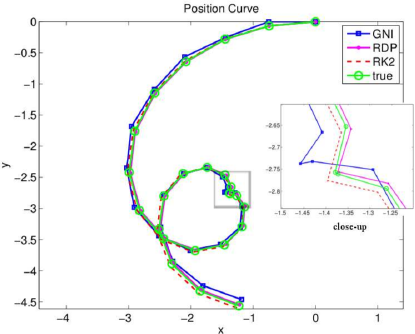
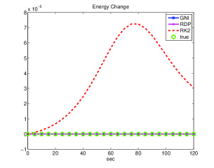
Figure 2. Position curves (left) of the sleigh integrators and the corresponding energy (right). The embedded close-up frame (left) zooms in on the cusp point of the “heart” shape.

Numerical Comparisons.

The numerical behavior of the algorithms is now examined in terms of their ability to reproduce the true system trajectory and in terms of their energy preservation. Comparison to a standard Runge-Kutta second-order method is also included.

Note that the standard Chaplygin sleigh model (e.g.  [1, 10, 12]) is studied in terms of the coordinates of the skate contact rather than the center off mass as in this work. For easier reference to such previous studies, we present the position curves below in terms of the skate coordinates $(x_{s},y_{s})$. This representation enables the generation of the familiar “heart”-shaped curves (Fig. 2).

6.2. The Snakeboard

The snakeboard (Fig. 3) represents a type of system with an interesting interplay between constraints and symmetries. It has served as a classical example (e.g. [2, 7, 4]) of a system with non-trivial intersection of the constraint distribution $\mathcal{D}$ and the vertical space $\mathcal{V}$. Our integrators capture the dynamics of such systems and their performance is examined in this section.

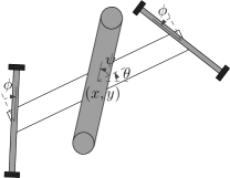
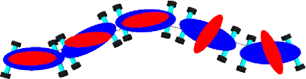
Figure 3. Snakeboard model (left) and a typical trajectory (right).

The shape space variables of the snakeboard are $r=(\psi,\phi)\in\mathrm{S}^{1}\times\mathrm{S}^{1}$ denoting the rotor angle and the steering wheels angle, while its configuration is defined by $(\theta,x,y)$ denoting orientation and position of the board. This corresponds to a configuration space $Q=\mathrm{S}^{1}\times\mathrm{S}^{1}\times\operatorname{SE}(2)$ with shape space $M=\mathrm{S}^{1}\times\mathrm{S}^{1}$ and group $G=\operatorname{SE}(2)$. Additional parameters are its mass $m$, distance $l$ from its center to the wheels, and moments of inertia $I$ and $J$ of the board and the steering. The kinematic constraints of the snakeboard are:

(34) $$\begin{split}&-l\cos\phi d\theta-\sin(\theta+\phi)dx+\cos(\theta+\phi)dy=0,\\ &l\cos\phi d\theta-\sin(\theta-\phi)dx+\cos(\theta-\phi)dy=0,\end{split}$$

enforcing the fact that the system must move in the direction in which the wheels are pointing and spinning. The constraint distribution is spanned by three covectors:

$$\mathcal{D}_{q}=\operatorname{span}\left\{\frac{\partial}{\partial\psi},\frac{\partial}{\partial\phi},c\frac{\partial}{\partial\theta}+a\frac{\partial}{\partial x}+b\frac{\partial}{\partial y}\right\},$$

where $a=-2l\cos\theta\cos^{2}\phi,\;b=-2l\sin\theta\cos^{2}\phi,\;c=\sin 2\phi$. The group directions defining the vertical space are:

$$\mathcal{V}_{q}=\operatorname{span}\left\{\frac{\partial}{\partial\theta},\frac{\partial}{\partial x},\frac{\partial}{\partial y}\right\},$$

and therefore the constrained symmetry space becomes:

(35) $$\mathcal{S}_{q}=\mathcal{V}_{q}\cap\mathcal{D}_{q}=\operatorname{span}\left\{c\frac{\partial}{\partial\theta}+a\frac{\partial}{\partial x}+b\frac{\partial}{\partial y}\right\}.$$

Since $\mathcal{D}_{q}=\mathcal{S}_{q}\oplus\mathcal{H}_{q},$ we have $\mathcal{H}_{q}=\operatorname{span}\left\{\frac{\partial}{\partial\psi},\frac{\partial}{\partial\phi}\right\}.$ Finally, the Lagrangian of the system is $L(q,\dot{q})=\frac{1}{2}\dot{q}^{T}M\dot{q}$ where

$$\operatorname{M}=\left[\begin{array}[]{ccccc}I&0&I&0&0\\ 0&2J&0&0&0\\ I&0&ml^{2}&0&0\\ 0&0&0&m&0\\ 0&0&0&0&m\end{array}\right].$$

The reduced Lagrangian can be expressed as $\ell(r,u,\xi)=(u,\xi)^{T}\operatorname{M}\;(u,\xi)$ by treating the velocity $\xi$ as a vector in the standard $\mathfrak{se}(2)$ basis (defined in App. B).

There is only one direction along which snakeboard motions lead to momentum conservation: it is defined by the basis element

$$e_{1}(r)=2l\cos^{2}\phi\left[\begin{array}[]{c}\frac{\tan\phi}{l}\\ -1\\ 0\end{array}\right],$$

and, hence, there is only one momentum variable $p_{1}\!=\!\big{\langle}\frac{\partial\ell}{\partial\xi},e_{1}(r)\big{\rangle}$. Using this variable we can derive the connection according to [2] as

$$[\mathcal{A}]=\left[\begin{array}[]{cc}\frac{I}{ml^{2}}\sin^{2}\phi&0\\ -\frac{I}{2ml}\sin 2\phi&0\\ 0&0\end{array}\right],\text{and }\quad\Omega=\frac{p_{1}}{4ml^{2}\cos^{2}\phi}e_{1}(r).$$

GNI Integrator.

The snakeboard constraints (34) can be expressed in terms of the one-forms

$$\mu_{1}(q)=(0,0,a,-c,0),\qquad\mu_{2}(q)=(0,0,b,0,-c).$$

The projector $\mathcal{Q}$ can then be computed from $\mu$ and the mass matrix $M$ using (12a) to obtain

$$\mathcal{Q}(q)=\frac{1}{ml^{2}\!-\!I\sin^{2}\phi}\left(\begin{array}[]{ccccc}0&0&-m(a^{2}\!+\!b^{2})&mac&mbc\\ 0&0&0&0&0\\ 0&0&m(a^{2}\!+\!b^{2})&-mac&-mbc\\ 0&0&-I^{\prime}ac&mb^{2}\!+\!I^{\prime}c^{2}&-mab\\ 0&0&-I^{\prime}bc&-mab&ma^{2}\!+\!I^{\prime}c^{2}\end{array}\right),$$

where $I^{\prime}=ml^{2}-I$ and $q=(\psi,\phi,\theta,x,y)$. Similarly to the Chaplygin sleigh §6.1, since the mass matrix is constant, the discrete dynamics is updated explicitly through $v_{k+\frac{1}{2}}=(\text{Id}-M^{-1}\mathcal{Q}(q_{k})^{T}M)v_{k-\frac{1}{2}}$.

RDP Integrator.

The reduced discrete equations of motion will be derived by substituting the Lagrangian and the connection of the snakeboard into (27) and choosing the map $\tau=\exp$. Since, particularly for the snakeboard, $\mathfrak{s}$ is one dimensional and $\mathcal{A}(r)\cdot\delta$ is parallel to $e_{1}(r)$ for any $\delta\in T_{r}M$ the discrete dynamics simplifies (see [17, 16]) to

$$\left\langle p_{k}-p_{k-1},e_{1}(r_{k})\right\rangle=0,\qquad\partial_{u}\ell_{k+\alpha}-\partial_{u}\ell_{k-1+\alpha}=0,$$

where

$$p_{k}=(ml^{2}\xi_{k}^{1}+Iu^{\phi}_{k},m\xi^{2}_{k},0),\qquad\partial_{u}\ell_{k}=(I(u^{\psi}_{k}+\xi^{1}_{k}),2Ju^{\phi}_{k}),$$

and the dynamics is derived by expressing $\xi_{k}=\Omega_{k}-\mathcal{A}(r_{k+\alpha})\cdot u_{k}$ in terms of $r_{k}=(\psi_{k},\phi_{k})$, $u_{k}=(u^{\psi}_{k},u^{\phi}_{k})$, and $(p_{1})_{k}$. Note that the discrete dynamics is linear in the unknowns $u_{k}$ and $(p_{1})_{k}$ and results in an efficient explicit integrator. The reconstruction equations are

$$g_{k+1}=g_{k}\exp(h\xi_{k}),\qquad r_{k+1}-r_{k}=hu_{k}.$$

Numerical Behavior.

The studied snakeboard integrators are second-order methods. Their advantage over similar methods is shown through comparison to a typical second order Runge-Kutta method as well as to the actual true trajectory. Fig. 4 shows a trajectory with initial conditions $\psi(0)=\pi/2$, $\phi(0)=\pi/3$, $p_{1}(0)=-1$, $\dot{\psi}(0)=2.5$, $\dot{\phi}(0)=-0.02$, $\theta(0)=0$. Sinusoidal control inputs $u_{\psi}=\cos(20\pi t)$, $u_{\phi}=\sin(2\pi t)$ at the joints were used to create parallel parking maneuvers with cusp points. The CPU run-times of the compared methods are nearly identical and are not included in the plots.

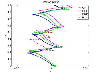
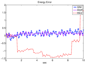
Figure 4. Snakeboard integrator numerics with $N=128$ timesteps over the integration horizon $T=10$ sec. At such coarse resolution RK2 method fails to follow the true trajectory while GNI and RDP have qualitatively correct behavior (position curve on left). One likely explanation lies in their better energy behavior (shown on right).

In special cases, for particular combinations of initial conditions and inertial parameters, the GNI integrator has shown non-physical oscillatory behavior. While this issue is most likely related to instabilities known to occur in projection-based methods, the exact cause remains to be determined in future work.

7. Conclusion

In this paper we have compared two geometric integrators for nonholonomic dynamics, the so-called GNI and RDP integrators. Both are constructed using differential geometric tools developed by geometric mechanics community through a careful study of nonholonomic dynamics during the last twenty years. This paper shows the importance of combining different research areas (differential geometry, numerical analysis and mechanics) to produce methods with an extraordinary qualitative and quantitative behavior.

Such issues raise a number of future work directions. We therefore close with some open questions:

• Given one of the nonholonomic integrators (GNI or RDP), does there exist, in the sense of backward error analysis, a continuous nonholonomic system, such that the discrete evolution for the nonholonomic integrator is the flow of this nonholonomic system up to an appropriate order?

• Is it possible to use the nonholonomic Hamilton-Jacobi theory recently developed [15, 19] for the construction of these methods or new ones?

These questions will be part of the future work that we will develop in the next years.

Appendix

Appendix A Retraction map tangents

The two common choices for retraction maps are the exponential map $\tau=\exp$ and the Cayley map $\tau=\operatorname{cay}$. In this section we provide their right-trivialized tangents $\operatorname{d}\tau$ of these maps and their inverses $\operatorname{d}\tau^{-1}$ (see [3] for more details).

A.1. Exponential map

The right-trivialized derivative of the map $\exp$ and its inverse are defined as

(36) $$\operatorname{dexp}_{x}y=\sum_{j=0}^{\infty}\frac{1}{(j+1)!}\operatorname{ad}_{x}^{j}y,\quad\operatorname{dexp}^{-1}_{x}y=\sum_{j=0}^{\infty}\frac{B_{j}}{j!}\operatorname{ad}_{x}^{j}y,$$

where $B_{j}$ are the Bernoulli numbers. Typically, these expressions are truncated in order to achieve a desired order of accuracy. The first few Bernoulli numbers are $B_{0}=1$, $B_{1}=-1/2$, $B_{2}=1/6$, $B_{3}=0$ (see [6, 13] for more details).

A.2. Cayley map

The derivative maps become (see [13] for derivation)

(37) $$\operatorname{dcay}_{x}y=\left(\operatorname{I}-\frac{x}{2}\right)^{-1}y\left(\operatorname{I}+\frac{x}{2}\right)^{-1},\quad\operatorname{dcay}^{-1}_{x}y=\left(\operatorname{I}-\frac{x}{2}\right)y\left(\operatorname{I}+\frac{x}{2}\right).$$

Appendix B Retraction Maps on $\mathrm{SE}(2)$

The coordinates of $\operatorname{SE}(2)$ are $(\theta,x,y)$ with matrix representation $g\in\operatorname{SE}(2)$ given by:

(41) $$g=\left[\begin{array}[]{ccc}\cos\theta&-\sin\theta&x\\ \sin\theta&\cos\theta&y\\ 0&0&1\end{array}\right].$$

Using the isomorphic map $\widehat{\cdot}:\mathbb{R}^{3}\rightarrow\mathfrak{se}(2)$ given by:

$$\widehat{v}=\left[\begin{array}[]{ccc}0&-v^{1}&v^{2}\\ v^{1}&0&v^{3}\\ 0&0&0\end{array}\right]\text{ for }v=\begin{pmatrix}\!v^{1}\!\\ \!v^{2}\!\\ \!v^{3}\!\end{pmatrix}\in\mathbb{R}^{3},$$

$\{\widehat{e}_{1},\widehat{e}_{2},\widehat{e}_{3}\}$ can be used as a basis for $\mathfrak{se}(2)$, where $\{e_{1},e_{2},e_{3}\}$ is the standard basis of $\mathbb{R}^{3}$.

The two maps $\tau:\mathfrak{se}(2)\rightarrow\operatorname{SE}(2)$ are given by

$$\exp(\widehat{v})\!=\!\!\left\{\!\!\begin{array}[]{cc}\!\!\left[\!\!\begin{array}[]{ccc}\cos v^{1}\!\!&\!\!-\sin v^{1}\!\!&\!\!\frac{v^{2}\sin v^{1}-v^{3}(1-\cos v^{1})}{v^{1}}\\ \sin v^{1}\!\!&\!\!\cos v^{1}\!\!&\!\!\frac{v^{2}(1-\cos v^{1})+v^{3}\sin v^{1}}{v^{1}}\\ 0\!\!&\!\!0\!\!&\!\!1\end{array}\!\!\right]\!\!&\!\!\text{if }v^{1}\neq 0\\ \left[\begin{array}[]{ccc}1&0&v^{2}\\ 0&1&v^{3}\\ 0&0&1\end{array}\right]\!\!&\!\!\text{if }v^{1}=0\end{array}\right.$$

$$\operatorname{cay}(\widehat{v})\!=\!\!\left[\!\!\begin{array}[]{ccc}\frac{1}{4+(v^{1})^{2}}\left[\!\!\begin{array}[]{ccc}(v^{1})^{2}\!-4&-4v^{1}&-2v^{1}v^{3}+4v^{2}\\ 4v^{1}&(v^{1})^{2}\!-4&2v^{1}v^{2}+4v^{3}\end{array}\!\!\right]\\ \begin{array}[]{ccc}0&\qquad 0&\qquad 1\end{array}\end{array}\!\!\right]$$

The maps $[\operatorname{d\tau}_{\xi}^{-1}]$ can be expressed as the $3\times 3$ matrices:

(42) $$[\operatorname{dexp}^{-1}_{\widehat{v}}]\approx\mathbf{I}_{3}-\frac{1}{2}[\operatorname{ad}_{v}]+\frac{1}{12}[\operatorname{ad}_{v}]^{2},$$

(44) $$[\operatorname{dcay}^{-1}_{\widehat{v}}]=\mathbf{I}_{3}-\frac{1}{2}[\operatorname{ad}_{v}]+\frac{1}{4}\left[\begin{array}[]{cc}v^{1}\cdot v&\mathbf{0}_{3\times 2}\end{array}\right],$$

where

$$[\operatorname{ad}_{v}]=\left[\begin{array}[]{ccc}0&0&0\\ v^{3}&0&-v^{1}\\ -v^{2}&v^{1}&0\end{array}\right].$$

References

- [1] Anthony M. Bloch. Nonholonomic mechanics and control, volume 24 of Interdisciplinary Applied Mathematics. Springer-Verlag, New York, 2003.
- [2] Anthony M. Bloch, P. S. Krishnaprasad, Jerrold E. Marsden, and Richard M. Murray. Nonholonomic mechanical systems with symmetry. Arch. Rational Mech. Anal., 136(1):21–99, 1996.
- [3] Nawaf Bou-Rabee and Jerrold E. Marsden. Hamilton-Pontryagin integrators on Lie groups. I. Introduction and structure-preserving properties. Found. Comput. Math., 9(2):197–219, 2009.
- [4] Francesco Bullo and Andrew D. Lewis. Geometric control of mechanical systems, volume 49 of Texts in Applied Mathematics. Springer-Verlag, New York, 2005. Modeling, analysis, and design for simple mechanical control systems.
- [5] Frans Cantrijn, Jorge Cortés, Manuel de León, and David Martín de Diego. On the geometry of generalized Chaplygin systems. Math. Proc. Cambridge Philos. Soc., 132(2):323–351, 2002.
- [6] Elena Celledoni and Brynjulf Owren. Lie group methods for rigid body dynamics and time integration on manifolds. Comput. Methods Appl. Mech. Engrg., 192(3-4):421–438, 2003.
- [7] Hernán Cendra, Jerrold E. Marsden, and Tudor S. Ratiu. Geometric mechanics, Lagrangian reduction, and nonholonomic systems. In Mathematics unlimited—2001 and beyond, pages 221–273. Springer, Berlin, 2001.
- [8] Jorge Cortés and Sonia Martínez. Non-holonomic integrators. Nonlinearity, 14(5):1365–1392, 2001.
- [9] Jorge Cortés Monforte. Geometric, control and numerical aspects of nonholonomic systems, volume 1793 of Lecture Notes in Mathematics. Springer-Verlag, Berlin, 2002.
- [10] Yuri N. Fedorov and Dmitry V. Zenkov. Discrete nonholonomic LL systems on Lie groups. Nonlinearity, 18(5):2211–2241, 2005.
- [11] S. Ferraro, D. Iglesias, and D. Martín de Diego. Numerical and geometric aspects of the nonholonomic shake and rattle methods. In AIMS Proceedings. (To appear).
- [12] S. Ferraro, D. Iglesias, and D. Martín de Diego. Momentum and energy preserving integrators for nonholonomic dynamics. Nonlinearity, 21(8):1911–1928, 2008.
- [13] Ernst Hairer, Christian Lubich, and Gerhard Wanner. Geometric numerical integration, volume 31 of Springer Series in Computational Mathematics. Springer-Verlag, Berlin, 2002.
- [14] David Iglesias, Juan C. Marrero, David Martín de Diego, and Eduardo Martínez. Discrete nonholonomic Lagrangian systems on Lie groupoids. J. Nonlinear Sci., 18(3):221–276, 2008.
- [15] David Iglesias-Ponte, Manuel de León, and David Martín de Diego. Towards a Hamilton-Jacobi theory for nonholonomic mechanical systems. J. Phys. A, 41(1):015205, 14, 2008.
- [16] Marin Kobilarov, Keenan Crane, and Mathieu Desbrun. Lie group integrators for animation and control of vehicles. ACM Transactions on Graphics, 28(2), April 2009.
- [17] Marin Kobilarov, Jerrold Marsden, and Gaurav Sukhatme. Geometric discretization of nonholonomic systems with symmetries. Discrete Contin. Dyn. Syst. Ser. S, 3(1):61–84, 2010.
- [18] Jair Koiller. Reduction of some classical nonholonomic systems with symmetry. Arch. Rational Mech. Anal., 118(2):113–148, 1992.
- [19] Manuel de León, Juan C. Marrero, and David Martín de Diego. Linear almost Poisson structures and Hamilton-Jacobi theory. Applications to nonholonomic mechanics. 2008. Preprint, arXiv:0801.4358.
- [20] Manuel de León and David Martín de Diego. On the geometry of non-holonomic Lagrangian systems. J. Math. Phys., 37(7):3389–3414, 1996.
- [21] Juan C. Marrero, David Martín de Diego, and Eduardo Martínez. Discrete Lagrangian and Hamiltonian mechanics on Lie groupoids. Nonlinearity, 19(6):1313–1348, 2006. Corrigendum: Nonlinearity 19 (2006), no. 12, 3003–3004.
- [22] J. E. Marsden and M. West. Discrete mechanics and variational integrators. Acta Numer., 10:357–514, 2001.
- [23] R. McLachlan and M. Perlmutter. Integrators for nonholonomic mechanical systems. J. Nonlinear Sci., 16(4):283–328, 2006.
- [24] Yuri I. Neĭmark and Nikolai A. Fufaev. Dynamics of Nonholonomic Systems. Translations of Mathematical Monographs, Vol. 33. American Mathematical Society, Providence, R.I., 1972.
- [25] George W. Patrick. Lagrangian mechanics without ordinary differential equations. Rep. Math. Phys., 57(3):437–443, 2006.
- [26] Jean-Paul Ryckaert, Giovanni Ciccotti, and Herman J. C. Berendsen. Numerical integration of the cartesian equations of motion of a system with constraint: molecular dynamics of -alkanes. J. Comput. Physics, 23:327–341, 1977.
- [27] J. M. Sanz-Serna and M. P. Calvo. Numerical Hamiltonian problems, volume 7 of Applied Mathematics and Mathematical Computation. Chapman & Hall, London, 1994.
- [28] Anatoly M. Vershik and L. D. Faddeev. Differential geometry and Lagrangian mechanics with constraints. Sov. Phys. Dokl., 17:34–36, 1972.