Integral equation models for thermoacoustic imaging of dissipative tissue

Abstract

In case of non-dissipative tissue the inverse problem of thermoacoustic imaging basically consists of two inverse problems. First, a function $\phi$ depending on the electromagnetic absorption function, is estimated from one of three types of projections (spherical, circular or planar) and secondly, the electromagnetic absorption function is estimated from $\phi$. In case of dissipative tissue, it is no longer possible to calculate explicitly the projection of $\phi$ from the respective pressure data (measured by point, planar or line detectors). The goal of this paper is to derive for each of the three types of pressure data, an integral equation that allows estimating the respective projection of $\phi$. The advantage of this approach is that all known reconstruction formulas for $\phi$ from the respective projection can be exploited.

1 Introduction

The goal of thermoacoustic imaging is to estimate the electromagnetic absorption function of soft tissue so that the strong contrast between the electromagnetic absorption of cancer and normal tissue can be exploited (cf. [13, 15, 18, 21, 28, 34]). Another advantage of thermoacoustic imaging is that the technological advance allows measuring different types of data (cf. [25, 7, 1, 34]) and therefore various explicit reconstruction formulas can be applied (cf. [5, 9, 14, 15, 29, 30, 31, 33]). In order to increase the resolution of thermoacoustic imaging, we derive integral equation models that take dissipation into account (cf. [2, 19, 20]) and allow the application of all known reconstruction formulas. In the following we explain this more precisely in case of point detectors.

First we discuss shortly the direct problem. The direct problem models the propagation of a pressure wave in dissipative tissue generated by very short heating of the tissue due to a laser. In case of homogeneous and isotropic dissipation, the direct problem can be modeled as follows (cf. Theorem 4.2.1 in [8])

(1) $$p=G*_{\mathbf{x},t}f\qquad\quad\mbox{($*_{\mathbf{x},t}$ space-time-convolution)}\,,$$

where $G$ corresponds to an attenuated spherical wave with origin in $(\mathbf{x},t)=({\mathbf{0}},0)$ and $f$ corresponds to the source term of $p$. In the absence of attenuation, $G$ is the retarted Green function of the standard wave with source term $f$. If $G$ is modeled appropriately, then $f$ is the same sorce term as in the absence of dissipation (cf. Section 2 and [21]), i.e.

(2) $$f(\mathbf{x},t)=\frac{\partial I(t)}{\partial t}\,\phi(\mathbf{x})\qquad\quad\mbox{($I$ short time impulse)}\,,$$

where $\phi$ depends on the electromagnetic absorption function, say $\phi=F(\alpha_{el})$. The essential requirement for $G$ is causality, i.e. the speed of the wave front (cf. [12])

$$\{(\mathbf{x},T(\mathbf{x}))\in{\mathbb{R}}^{4}\,|\,T(\mathbf{x}):=\sup\{t>0\,|\,G(\mathbf{x},\tau)=0\mbox{ for all }\tau\leq t\}\,$$

has to be bounded from above. Here $T(|\mathbf{x}|)$ denotes the travel time of the wave front. Below we will see that causality plays an important role in thermoacoustic imaging.

The respective inverse problem can be formulated as follows. Let $\Gamma$ denote a surface covered with point detectors surrounding the tissue. From (1) and (2), we obtain the integral equation

(3) $$\int_{{\mathbb{R}}^{3}}\tilde{G}(\mathbf{x}-\mathbf{y},t)\,\phi(\mathbf{y})\,{\rm d}\mathbf{y}=p(\mathbf{x},t)\qquad\mbox{ for}\quad\mathbf{x}\in\Gamma,\,t\in[0,T]\,,$$

where $\tilde{G}:=G*_{t}\frac{\partial I(t)}{\partial t}$ and $T$ is sufficiently large. The inverse problem corresponds to the estimation of $\phi$ in integral equation (3) and the subsequent inversion of $\phi=F(\alpha_{el})$.

In this paper we show that integral equation (3) can be reformulated to

(4) $$\int_{0}^{\infty}N(t,t^{\prime})\,R_{sp}(\phi)(\mathbf{x},t^{\prime})\,{\rm d}t^{\prime}=p(\mathbf{x},t)\qquad(N\in C^{\infty}({\mathbb{R}}^{2}\backslash\{(0,0)\})\,,$$

where $R_{sp}(\phi)$ denotes the spherical projection of $\phi$, i.e.

(5) $$R_{sp}(\phi)(\mathbf{x},t):=\int_{\partial B_{t}(\mathbf{x})}\phi(\mathbf{x}^{\prime})\,{\rm d}\lambda^{2}(\mathbf{x}^{\prime})\qquad\quad\mathbf{x}\in{\mathbb{R}}^{3},t\geq 0\,.$$

Here ${\rm d}\lambda^{2}$ denotes the Lebesgue measure on ${\mathbb{R}}^{2}$. The causality of $G$ ensures that $N(t,t^{\prime})=0$ if $t^{\prime}>t$, i.e. the upper integration limit in (4) can be replaced by $t$. This means that the pressure function does not depend on information from the future. For some surfaces $\Gamma$, $\phi$ can be reconstructed from $R_{sp}(\phi)$ via exact or approximate explicit reconstruction formulas. For example, if $\Gamma$ is a sphere, then (cf. e.g. [14, 15])

(6) $$\phi(\mathbf{x})=-\frac{1}{2\,\pi}\,\mbox{div}\,\int_{S^{2}}{\mathbf{n}}(\mathbf{x}^{\prime})\left[\frac{\partial}{\partial t}\left(t\,R_{sp}(\phi)(\mathbf{x}^{\prime},t)\right)\right]_{t=|\mathbf{x}^{\prime}-\mathbf{x}|}{\rm d}\lambda^{2}(\mathbf{x}^{\prime})\,,$$

where ${\mathbf{n}}$ denotes the exterior normal of $S^{2}$. In the absence of attenuation, if $I(t)=\delta(t)$, then the projection $R_{sp}(\phi)$ can be calculated explicitly from (cf. [10])

(7) $$\frac{\partial}{\partial t}\left(\frac{R_{sp}(\phi)(\mathbf{x},t)}{4\,\pi\,t}\right)=p_{0}(\mathbf{x},t)\qquad\mbox{ ($p_{0}$ unattenuated data)}\,.$$

However, in the presence of attenuation, a set of $1d-$integral equations like (4) has to be solved to obtain the projection $R_{sp}(\phi)$. Moreover, we see that if an efficient and accurate explicit reconstruction formula for $\phi$ from data $R_{sp}(\phi)$ exists, then the iterative estimation of $\phi$ via integral equation (3) is unfavorable. The goal of this paper is to derive $1d-$integral equations that relate spherical, circular and planar projections to attenuated pressure data measured by point, line and planar detectors, respectively. We note that this is a theoretical paper that is not concerned with numerical experiments.

The outline of this paper is as follows. The direct problem of thermoacoustic imaging of dissipative tissue is modeled in Section 2. In Section 3 an integral equation model is derived that allows the estimation of the unattenuated pressure data in case $I(t)=\delta(t)$. Then, from this model, the basic theorem of thermoacoustic imaging of dissipative tissue is derived in case $I(t)\not=\delta(t)$. Subsequently, in Section 4, integral equation models for the three types of projections are derived that allow applying the explicit reconstruction formulas of thermoacoustic tomography. In the appendix it is proven that the wave equation modeled in Section 2 has a unique Green function satisfying the “initial condition” $G|_{t<0}=0$ and causality, defined as in Section 2.

2 Modeling of the direct problem

In this section we model the direct problem of thermoacoustic imaging of dissipative tissue. First we summarize essential facts about wave attenuation and causality and then model the stress tensor and the source term for thermoacoustic imaging of dissipative tissue. For more details we refer to [12, 17, 19, 22, 23, 24].

Causal wave attenuation in tissue

Consider a viscous medium that is homogeneous with respect to density, compressibility and attenuation. Then pressure waves obeying a complex attenuation law $\alpha_{*}=\alpha_{*}(\omega)$ satisfy the wave equation (cf. [12])

(8) $$\nabla^{2}p_{\gamma}(\mathbf{x},t)-\left(D_{*}+\frac{1}{c_{0}}\,\frac{\partial}{\partial t}\right)^{2}p_{\gamma}(\mathbf{x},t)=-f(\mathbf{x},t)\,,$$

where $c_{0}>0$ is a constant and $D_{*}$ is a time convolution operator with kernel defined by

$$\hat{K}_{*}(\omega):=\frac{\alpha_{*}(\omega)}{\sqrt{2\,\pi}}\qquad\qquad\mbox{($\hat{\;}$ denotes Fourier transform)}\,.$$

The functions $\alpha_{*}:{\mathbb{R}}\to{\mathbb{C}}$ is called complex attenuation law and $\alpha:=\mbox{Re}(\alpha_{*})$ is called (real) attenuation law. In order that $p_{\gamma}$ is real valued $\alpha$ must be even and $\mbox{Im}(\alpha_{*})$ must be odd. Attenuation occurs only if $\alpha$ is positive. Moreover, the function $\alpha_{*}$ is restrained by the requirement of a bounded wave front speed of the Green function $G_{\gamma}$ of (8) (causality). If the wave front speed this is bounded from above by $c_{1}\in(0,\infty)$, then this is equivalent to

$$G_{\gamma}\left(\mathbf{x},t+T(|\mathbf{x}|)\right)=0\quad\mbox{ if }\quad t<0\quad\mbox{ for all }\mathbf{x}\not=0\,,$$

where $T(|\mathbf{x}|)\in(|\mathbf{x}|/c_{1},\infty)$ is the travel time of the wave front from point ${\mathbf{0}}$ to point $\mathbf{x}$. In case of a constant wave front speed $c_{0}$, causality is equivalent to

(9) $$K(\mathbf{x},t):=4\,\pi\,|\mathbf{x}|\,G_{\gamma}\left(\mathbf{x},t+\frac{|\mathbf{x}|}{c_{0}}\right)=0\quad\mbox{ if }\quad t<0\quad\mbox{ for all }\mathbf{x}\not=0\,.$$

since $T(|\mathbf{x}|)=|\mathbf{x}|/c_{0}$. We note that $\hat{K}(\mathbf{x},\omega)=e^{-\alpha_{*}(\omega)\,|\mathbf{x}|}/\sqrt{2\,\pi}$ (cf. Theorem 9 in the appendix).

Remark 1.

In the literature often a less strong definition of causality is used that demands the existence of a (retarted) Green function that vanishes for $t<0$. However, this requirement is not related to the speed of the wave front.

According to experiments the real attenuation law of a variety of viscous media similar to tissue satisfy (at least approximately) a frequency power law (cf. [24, 27]).

$$\alpha(\omega)=\alpha_{0}\,|\omega|^{\gamma}\qquad\mbox{ for }\qquad\gamma\in(1,2]\,,\quad\mbox{$\alpha_{0}=$const.}$$

This led to the complex attenuation laws (cf. [22, 23, 24, 26])

(10) $$\alpha_{*}(\omega)=\tilde{\alpha}_{0}\,(-{\mathrm{i}}\,\omega)^{\gamma}\qquad\mbox{ with }\qquad\tilde{\alpha}_{0}:=\frac{\alpha_{0}}{\cos(\pi\,\gamma/2)}\,,$$

which violate causality for the range $\gamma\in(1,2]$ relevant for thermoacoustic imaging (cf. appendix). For thermoacoustic imaging we propose the following complex attenuation laws

(11) $$\alpha_{*}(\omega)=\frac{\alpha_{0}\,(-{\mathrm{i}}\,\omega)}{c_{0}\,\sqrt{1+(-{\mathrm{i}}\,\tau_{0}\,\omega)^{\gamma-1}}}\qquad\qquad(\gamma\in(1,2],\,\tau_{0}>0)\,,$$

where the square root of $1+(-{\mathrm{i}}\,\tau_{0}\,\omega)^{\gamma-1}$ is understood as the root that guarantees a nonnegative real part of $\alpha_{*}$.

Remark 2.

We note that the above complex power function is defined by

(12) $$w^{\gamma}=e^{\gamma\,\left(\mbox{log}(r)+{\mathrm{i}}\,\varphi\right)}\qquad\mbox{ for }\qquad w=r\,e^{{\mathrm{i}}\,\varphi}\in C^{-}\,,$$

where $C^{-}:={\mathbb{C}}\backslash\{z\in{\mathbb{C}}\,|\,\mbox{Re}(z)\leq 0,\,\mbox{Im}(z)=0\}$.

Remark 3.

In the appendix we prove that the Green function $G_{\gamma}$ of (8) with $\alpha_{*}$ defined as in (10) does not satisfy the causality requirement (9), but if $\alpha_{*}$ is defined as in (11) then (9) is satisfied (cf. [12]). Models (11) are appropriate for thermoacoustic imaging, since causality is satisfied and $\mbox{Re}(\alpha_{*})$ is approximately a frequency power law with exponent $\gamma\in(1,2]$ for small frequencies (cf. Figure 1). If $\gamma=2$ then $\mbox{Re}(\alpha_{*})$ is the thermo-viscous attenuation law.

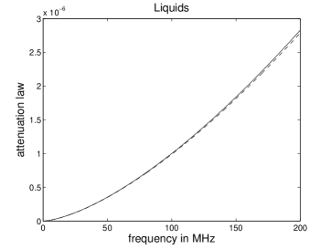
Figure 1: Comparison of the real part of (11) with $\alpha_{0}:=\frac{2\,c_{0}\,\tau_{0}}{|cos(\pi\,\gamma/2)|}$ (dashed line) and the power law $\alpha(\omega)=|\tau_{0}\,\omega|^{\gamma}$ for $\gamma=1.5$. For liquids: $\tau_{0}=10^{-6}\,MHz$ (left picture) and for gases: $\tau_{0}=10^{-4}\,MHz$ (right picture) (cf. [11]). Experimental demonstrations of the power law are performed for the range $0-60\,MHz$ (cf. e.g. [24]).

Remark 4.

All mathematical results in this paper are valid if $\alpha_{*}$ defined as in (11) is replaced by a complex attenuation law that satisfies (9) and has a monotonic increasing real part.

Modeling of the stress tensor and the source term

Since equation (8) is an integro-differential equation, it is not self-evident that the source term $f$ has the same structure as in the absence of wave attenuation. In order to model the source term we first model the temperature dependent stress tensor.

According to [16] the stress tensor of an invisid fluid can be modeled by

$$\sigma_{i,j}=-c_{0}^{2}\,\rho_{0}\,\alpha_{th}\,(T-T_{0})\,\delta_{i,j}-p_{1}\,\delta_{i,j}\qquad\mbox{ where }\qquad p_{1}=p_{0}+c_{0}^{2}\,(\rho-\rho_{0})\,.$$

Here $p_{0}$, $\rho_{0}$, $c_{0}$, $T_{0}$ are reference values of the pressure, the density, the sound speed and the temperature, respectively, and $\alpha_{th}$ is the thermal expansion coefficient. Wave equation (8) shows that a dissipative medium has a long memory (cf. [3]) and therefore we claim that attenuation is accounted for if $\sigma_{i,j}$ is replaced by $K_{1}*_{t}\sigma_{i,j}$, where $*_{t}$ denotes time-convolution and $K_{1}$ is an appropriate kernel. We show that this ansatz implies wave equation (8) with the same thermoacoustic source term as in the absence of wave attenuation. (This calculation can be considered as another justification of model equation (8).) Since $\sigma_{1,1}=\sigma_{2,2}=\sigma_{3,3}$ correspond to the negative total pressure in the absence of dissipation, our claim implies

(13) $$p=\tilde{p}_{0}+c_{0}^{2}\,\,K_{1}*_{t}(\rho-\rho_{0})+c_{0}^{2}\,\rho_{0}\,\alpha_{th}\,K_{1}*_{t}(T-T_{0})$$

with $\tilde{p}_{0}:=p_{0}\,\int_{\mathbb{R}}K_{1}(t)\,{\rm d}t=\sqrt{2\,\pi}\,p_{0}\,\hat{K}_{1}(0+)$.

If the activation time of the laser is very short, say $\Delta t$, then the absorbed heat content of $\Omega$ at $t=\Delta t$ can be modeled by (cf. [6])

$$\Delta Q(\mathbf{x},\Delta t) =\alpha_{el}\,\epsilon_{0}(\mathbf{x})\,\int e^{-\alpha_{el}\,|\mathbf{x}-\mathbf{x}_{S}|}\,{\rm d}\mathbf{x}_{s}\,I(t)\,\Delta t$$

$$=:\alpha_{el}\,I_{0}(\alpha_{el},\mathbf{x})\,I(t)\,\Delta t,$$

where $\alpha_{el}$, $\epsilon_{0}$ and $\mathbf{x}_{s}$ denote the electromagnetic absorption coefficient, the absorbed energy flow density and the origin of an electromagnetic point source, respectively. Moreover, $I=I(t)$ denotes a short time pulse. On the other hand the heat content of the mass $m_{\Omega}$ within $\Omega$ due to the rise of temperature is

$$\Delta Q(\mathbf{x},\Delta t)=m_{\Omega}\,c_{p}\,(T(\mathbf{x},\Delta t)-T_{0}),$$

where $c_{p}$ denotes the specific heat capacity of $m_{\Omega}$ at constant pressure. In summary we get

(14) $$\,\frac{{\rm d}T}{dt}=\frac{\alpha_{el}\,I_{0}(\alpha_{el},\cdot)}{m_{\Omega}\,c_{p}}\,I.$$

Since a state equation refers always to the local comoving system, the total time derivative ${\rm d}/{\rm d}t$ appears. From (13) we infer the state equation

(15) $$\frac{1}{c_{0}^{2}}\,\frac{{\rm d}p}{{\rm d}t}=K_{1}*_{t}\frac{{\rm d}\rho}{{\rm d}t}+\rho_{0}\,\alpha_{th}\,K_{1}*_{t}\frac{{\rm d}T}{{\rm d}t}\,.$$

If the sound speed is not to large, then ${\rm d}/{\rm d}t$ can be replaced by $\partial/\partial t$. In the following we assume that this simplification is appropriate. The linearized equation of motion and the linearized continuity equation

$$\rho_{0}\,\frac{\partial{\mathbf{v}}}{\partial t}=-\nabla p\qquad\mbox{ and }\qquad\frac{\partial\rho}{\partial t}+\rho_{0}\,\nabla\cdot{\mathbf{v}}=0$$

imply

$$\nabla^{2}p-\frac{\partial^{2}\rho}{\partial t^{2}}=0\,.$$

From this, (15) and (14) we infer

(16) $$K_{1}(t)*_{t}\nabla^{2}p(\mathbf{x},t)-\frac{1}{c_{0}^{2}}\,\frac{\partial^{2}p(\mathbf{x},t)}{\partial t^{2}}=-K_{1}(t)*_{t}f(\mathbf{x},t)\,,$$

with

$$f=\frac{\alpha_{th}\,\alpha_{el}\,I_{0}(\alpha_{el},\cdot)}{|\Omega|\,c_{p}}\,\frac{\partial I}{\partial t}\qquad\quad\mbox{($|\Omega|$ volume of $\Omega$)}\,.$$

Comparison of (8) and (16) in Fourier space, shows that both equations are equivalent if

(17) $$\hat{K}_{1}(\omega):=\frac{1}{\sqrt{2\,\pi}}\,\left(\frac{\omega}{c_{0}\,k(\omega)}\right)^{2}\,,\qquad\qquad k(\omega):={\mathrm{i}}\,\alpha_{*}(\omega)+\frac{\omega}{c_{0}}\,.$$

Now we can formulate the direct problem.

The direct problem

Let $T,\,T_{1}>0$ with $T_{1}<<T$ and e.g. $\phi\in L^{2}(\Omega)$ and $I\in\mathcal{E}({\mathbb{R}})$ with $\mbox{supp}(I)\subset[0,T_{1}]$. The direct problem of thermoacoustic tomography is to solve wave equation (16) on ${\mathbb{R}}^{3}\times(0,T)$ with

(18) $$f(\mathbf{x},t):=\phi(\mathbf{x})\,I^{\prime}(t)\qquad\mbox{ where }\qquad\phi:=\frac{\alpha_{th}\,\alpha_{el}}{|\Omega|\,c_{p}}\,I_{0}$$

such that

(19) $$\left.p_{\gamma}\right|_{t<0}=0\,.$$

Let $\delta(t)$ denote the delta distribution. Frequently, it is assumed that $I(t)=\delta(t)$, since the speed of light is much larger than the speed of sound. Then we have

(20) $$f(\mathbf{x},t)=\phi(\mathbf{x})\,\delta^{\prime}(t)$$

and $\phi$ corresponds to an initial value function.

Remark 5.

In the appendix we show that wave equation (16) has a unique Green function $G_{\gamma}$ ($f(\mathbf{x},t)=\delta(\mathbf{x})\,\delta(t)$) satisfying $G_{\gamma}|_{t<0}=0$.

3 Derivation of the basic theorem

Before we explain the purpose of this section we introduce some important notions and assumptions.

• Without loss of generality we assume $c_{0}=1$. $\alpha_{*}$ is defined as in (11) if $\gamma\in(1,2]$ and $\alpha_{*}:=0$ if $\gamma=0$. Moreover, $k$ is defined as in (17).

• $p_{\gamma}$ is the unique solution of (16) with (19) and $f(\mathbf{x},t)=\phi(\mathbf{x})\,I^{\prime}(t)$ and $\tilde{p}_{0}$ is the unique solution of (16) with (19) and $f(\mathbf{x},t)=\phi(\mathbf{x})\,\delta^{\prime}(t)$.

If $I(t)\not=\delta(t)$, then we assume that the signal satisfies

• $I\in C({\mathbb{R}})$ and $\mbox{supp}(I)\subset[0,T_{1}]$ for some $T_{1}>0$.

If $I(t)=\delta(t)$ then $\tilde{p}_{0}=p_{0}$. The uniqueness of the Green function of (16) is proven in Theorem 9 in the appendix.

The goal of this section is to derive an integral equation that allows the estimation of $\tilde{p}_{0}$ from the data $p_{\gamma}$. This will be the basic theorem of thermoacoustic imaging of dissipative tissue.

The following two lemmas provide important properties of a distribution that plays an important role in deriving the basic theorem.

Lemma 1.

Let (A1) be satisfied and

(21) $$\hat{M}_{\gamma}(\omega,t^{\prime}) :=\frac{1}{\sqrt{2\,\pi}}\,\frac{\omega}{k(\omega)}\,e^{{\mathrm{i}}\,k(\omega)\,|t^{\prime}|}\qquad(\omega,\,t^{\prime}\in{\mathbb{R}})\,.$$

a) $M_{\gamma}$ satisfies for $t^{\prime}\geq 0$

(22) $$K_{1}*_{t}\frac{\partial^{2}M_{\gamma}}{\partial t^{\prime 2}}-\frac{\partial^{2}M_{\gamma}}{\partial t^{2}}=0\quad\mbox{ with }\quad\left.\frac{\partial M_{\gamma}}{\partial t^{\prime}}\right|_{t^{\prime}=0}=-\delta^{\prime}(t)$$

b) If $\alpha_{*}\not=0$ then $M_{\gamma}\in C^{\infty}({\mathbb{R}}^{2}\backslash\{(0,0)\})$.
c) If $\alpha_{*}=0$ then $M_{\gamma}(t,t^{\prime})=\delta(t-|t^{\prime}|)$.

Proof.

a) In Fourier space, equation (22) and definition (21) read as follows:

$$\frac{(-{\mathrm{i}}\,\omega)^{2}}{({\mathrm{i}}\,k(\omega))^{2}}\,\frac{\partial^{2}\hat{M}_{\gamma}(\omega,t^{\prime})}{\partial t^{\prime 2}}-(-{\mathrm{i}}\,\omega)^{2}\,\hat{M}_{\gamma}(\omega,t^{\prime})=0\,,$$

$$\frac{\partial^{2}\hat{M}_{\gamma}(\omega,t^{\prime})}{\partial t^{\prime 2}}=({\mathrm{i}}\,k(\omega))^{2}\,\hat{M}_{\gamma}(\omega,t^{\prime})\qquad t^{\prime}>0\,.$$

From both identities, it follows that $M_{\gamma}(t,t^{\prime})$ satisfies the first identity in (22). The second identity in (22) follows from (21):

$$\left.\frac{\partial M_{\gamma}(t,t^{\prime})}{\partial t^{\prime}}\right|_{t^{\prime}=0}=\mathcal{F}^{-1}\left\{\frac{{\mathrm{i}}\,\omega}{\sqrt{2\,\pi}}\,\right\}(t)=-\delta^{\prime}(t)\,.$$

b) Let $\alpha_{*}\not=0$. For fixed $|t^{\prime}|=T>0$, $M_{\gamma}$ can be considered as oscillatory integral (cf. Section 7.8 in [8])

$$I_{\phi,a}(u)=\int e^{{\mathrm{i}}\,\phi(t,\omega)}a(t,\omega)\,u(t){\rm d}t\,{\rm d}\omega\qquad u\in C^{\infty}_{0}({\mathbb{R}})$$

with phase function $\phi(t,\omega)=-t\,\omega$ in $\Gamma={\mathbb{R}}\times({\mathbb{R}}\backslash\{0\})$ and $a(t,\omega)=\frac{1}{\sqrt{2\,\pi}}\,\frac{\omega}{k(\omega)}\,e^{{\mathrm{i}}\,k(\omega)\,T}$, since $a$ is $C^{\infty}$ and rapidly decreasing with respect to $\omega$. From Theorem 7.8.3 in [8] and

$$\frac{{\rm d}\phi}{{\rm d}\omega}(t,\omega)=0\qquad\mbox{ iff }\qquad t=0\,,$$

it follows that $\mbox{sing\,supp\,}(I_{\phi,a})\subseteq\{0\}$. That is to say $M_{\gamma}(t,T)$ is $C^{\infty}$ for $t>0$. Similarly, if $t=T$ is fixed then it follows that $M_{\gamma}(T,t^{\prime})$ is $C^{\infty}$ for $|t^{\prime}|>0$. This shows that $M_{\gamma}$ is $C^{\infty}$ on ${\mathbb{R}}^{2}\backslash\{(0,0)\}$.
c) The claim follows from $k(\omega)=\omega$ ($\alpha_{*}=0$) and property $\mathcal{F}\{\delta(t-t^{\prime})\}(\omega)=e^{{\mathrm{i}}\,\omega\,t^{\prime}}/\sqrt{2\,\pi}$. This concludes the proof. ∎

Lemma 2.

Let (A1) be satisfied with $\alpha_{*}\not=0$ and $M_{\gamma}$ be defined as in (21).
a) If $t^{\prime}=0$ then

$$M_{\gamma}(t,0)=0\qquad\mbox{ for }\quad t<0\,.$$

b) If $t^{\prime}\not=0$ then $t\mapsto M_{\gamma}(t,t^{\prime})$ is a rapidly decreasing $C^{\infty}-$function on ${\mathbb{R}}$ and satisfies

(23) $$M_{\gamma}(t,t^{\prime})=0\qquad\mbox{ for }\quad t\leq|t^{\prime}|\,.$$

Proof.

a) From (21) with $t^{\prime}=0$ and (11) we get

$$\sqrt{2\,\pi}\,\hat{M}_{\gamma}(\omega,0)=\frac{\omega}{k(\omega)}=\frac{\sqrt{1+(-{\mathrm{i}}\,\tau_{0}\,\omega)^{\gamma-1}}}{\alpha_{0}+\sqrt{1+(-{\mathrm{i}}\,\tau_{0}\,\omega)^{\gamma-1}}}\qquad(\alpha_{0}>0)\,.$$

Here the power functions are defined on ${\mathbb{C}}\backslash(-\infty,0]$. Since $\alpha_{0}+\sqrt{1+(-{\mathrm{i}}\,\tau_{0}\,z)^{\gamma-1}}$ maps

$$\{z\in{\mathbb{C}}\,|\,\mbox{Im}(z)\geq 0\}\quad\mbox{ to }\quad\{w\in{\mathbb{C}}\,|\,\mbox{Re}(w)\geq\alpha_{0}\}\,,$$

we see that $\hat{M}_{\gamma}(z,0)$ is holomorphic for all $\mbox{Im}(z)\geq 0$. Hence conditions (C1) and (C2) of Theorem 6 in the appendix are satisfied. Moreover, we see that there exists a polynomial $P$ such that

$$|\hat{M}_{\gamma}(z,0)|\leq P(|z|)\qquad\mbox{ for }\qquad\mbox{Im}(z)\geq 0\,.$$

According to Theorem 6 in the appendix, $M_{\gamma}(t,0)$ vanishes for $t<0$.
b) Let $\alpha_{*}\not=0$. If $t^{\prime}\not=0$ is fixed, then $M_{\gamma}(\omega,t^{\prime})$ is rapidly decreasing and $C^{\infty}-$ and thus $M_{\gamma}(t,t^{\prime})$ is a rapidly decreasing $C^{\infty}-$function on ${\mathbb{R}}$. Hence property (23) is satsified if

(24) $$M_{\gamma}(t+|t^{\prime}|,t^{\prime})=0\qquad\mbox{ for }\quad t<0\,.$$

Because of (21) and the second definition in (17) we have

$$M_{\gamma}(t+|t^{\prime}|,t^{\prime})=\mathcal{F}^{-1}\left\{\hat{M}_{\gamma}(\omega,t^{\prime})\,e^{-{\mathrm{i}}\,\omega\,|t^{\prime}|}\right\}(t)=\mathcal{F}^{-1}\left\{\frac{\omega}{k(\omega)}\,\frac{e^{-\alpha_{*}(\omega)\,|t^{\prime}|}}{\sqrt{2\,\pi}}\,\right\}(t)$$

According to part a) of this proof and Theorem 8 in the appendix both functions

$$\mathcal{F}^{-1}\left\{\frac{\omega}{k(\omega)}\right\}(t)\quad\mbox{ and }\quad\mathcal{F}^{-1}\left\{\frac{e^{-\alpha_{*}(\omega)\,|t^{\prime}|}}{\sqrt{2\,\pi}}\,\right\}(t)$$

vanish for $t<0$ and therefore their convolution vanishes for $t<0$, too. This proves property (24) and concludes the proof. ∎

Let $\tau_{1},\,\tau_{2}\in{\mathbb{R}}$. We recall that if $f_{1}$ and $f_{2}$ are two distributions with support in $[\tau_{1},\infty)$ and $[\tau_{2},\infty)$, respectively, then $f_{1}*f_{2}$ is well-defined and (cf.  [8])

(25) $$\mbox{supp}(f_{1}*f_{2})\subseteq\mbox{supp}(f_{1})+\mbox{supp}(f_{2})\subseteq[\tau_{1}+\tau_{2},\infty)\,.$$

Now we derive the first integral relation that relates the attenuated pressure data with the unattenuated pressure data in case $I(t)=\delta(t)$. Note that in this case $p_{0}\equiv\tilde{p}_{0}$ (cf. (A2)).

Theorem 1.

Let (A1), (A2) with $I(t)=\delta(t)$ be satisfied and $M_{\gamma}$ be defined as in (21). Then $p_{0}$ solves the integral equation

(26) $$p_{\gamma}(\mathbf{x},t)=\int_{0}^{\infty}M_{\gamma}(t,t^{\prime})\,p_{0}(\mathbf{x},t^{\prime})\,{\rm d}t^{\prime}\,.$$

Here the upper limit of integration can be replaced by $t$.

Proof.

Let $t^{\prime}\geq 0$. From properties (22), (23) and (25), it follows that

(27) $$K_{1}(t)*_{t}\frac{\partial^{n}M_{\gamma}(t,t^{\prime})}{\partial t^{\prime n}}=0\qquad\mbox{ if }\qquad t\leq t^{\prime}\;\mbox{ and }\;n\in\{0,\,1\}\,.$$

Moreover, $p_{0}$ satisfies ($\gamma=0$, $K_{1}(t)=\delta(t)$)

(28) $$\nabla^{2}p_{0}(\mathbf{x},t^{\prime})=\frac{\partial^{2}p_{0}(\mathbf{x},t^{\prime})}{\partial t^{\prime 2}}\qquad\mbox{ for $t^{\prime}>0$}\,,$$

$$p_{0}(\cdot,0+)=\phi\qquad\mbox{ and }\qquad\frac{\partial p_{0}}{\partial t}(\cdot,0+)=0\,.$$

For convenience we introduce the notions

(29) $$\Box p:=K_{1}(t)*_{t}(\nabla^{2}p)-\frac{\partial^{2}p}{\partial t^{2}}$$

and

$$q(\mathbf{x},t):=\int_{0}^{\infty}M_{\gamma}(t,t^{\prime})\,p_{0}(\mathbf{x},t^{\prime})\,{\rm d}t^{\prime}\,.$$

Kernel property (23) implies that the upper limit can be replaced by $t$. From (22) we get

$$\Box q(\mathbf{x},t) =\int_{0}^{\infty}K_{1}(t)*_{t}\left[M_{\gamma}(t,t^{\prime})\,\nabla^{2}p_{0}(\mathbf{x},t^{\prime})-\frac{\partial M_{\gamma}(t,t^{\prime})}{\partial t^{\prime}}\,p_{0}(\mathbf{x},t^{\prime})\right]\,{\rm d}t^{\prime}\,,$$

which simplifies with integration by parts together with (27) and (28) to

(30) $$\Box q(\mathbf{x},t) =\phi(\mathbf{x})\,\left[K_{1}(t)*_{t}\frac{\partial M_{\gamma}(t,t^{\prime})}{\partial t^{\prime}}\right]_{t^{\prime}=0}=-\phi(\mathbf{x})\,\,\delta(t)*_{t}K_{1}(t)\,.$$

Because $p_{\gamma}$ is the unique solution of (16) satisfying (19) (cf. Theorem 9 in the appendix), it follows that $p_{\gamma}=q$. This concludes the proof. ∎

From Theorem 1, assumption (A3) and (25), we get:

Theorem 2.

Let (A1)-(A3) be satisfied and $M_{\gamma}$ be defined as in (21). Then $\tilde{p}_{0}$ solves the integral equation

(31) $$p_{\gamma}(\mathbf{x},t)=\int_{0}^{\infty}[I(t)*_{t}M_{\gamma}(t,t^{\prime})]\,\tilde{p}_{0}(\mathbf{x},t^{\prime})\,{\rm d}t^{\prime}\,.$$

The upper limit of integration can be replaced by $t$.

4 Integral equation models for projections of $\phi$

In this section we derive integral equation models for the three types of projections in thermoacoustic tomography. For various situations, the function $\phi$ can be calculated via explicit reconstruction formulas from projections of $\phi$ (cf. [5, 9, 14, 15, 29, 30, 31, 33]). In case of reconstructions with limited-view, we refer to [32] and the literature cited there.

In this section we use the following notions and assumptions:

• The region of interest (tissue) $\Omega\subset{\mathbb{R}}^{3}$ is a subset of the open ball $B_{R_{0}}({\mathbf{0}})$ with radius $R_{0}>0$.

• ${\rm d}\lambda^{m}$ denotes the Lebesgue measure on ${\mathbb{R}}^{m}$ for $m\in\{1,\,2,\,3\}$.

Case of Point detectors

The simplest setup of point detector, which guarantees stable reconstruction, is the sphere $\Gamma=\partial B_{R_{0}}({\mathbf{0}})$ that encloses the region of interest. Then the set of data is

$$\{p_{\gamma}(\mathbf{x},t)\,|\,\mathbf{x}\in\Gamma,\,t\in[0,T]\}\,\quad\qquad\mbox{($T>0$ sufficiently large)\,.}$$

Inserting the spherical mean representation (7) into integral equation (31) and performing integration by parts yield

$$p_{\gamma}(\mathbf{x},t)=-\int_{0}^{t}\frac{\partial}{\partial t^{\prime}}\,\left[I(t)*_{t}M_{\gamma}(t,t^{\prime})\right]\,\frac{R_{sp}(\phi)(\mathbf{x},t^{\prime})}{4\,\pi\,t^{\prime}}\,{\rm d}t^{\prime}\qquad\mbox{ for $t\geq 0$}\,,$$

since (25) holds and

$$\left[\frac{R_{sp}(\phi)(\mathbf{x},t^{\prime})}{4\,\pi\,t^{\prime}}\right]_{t^{\prime}=0}=\left[\int_{0}^{t^{\prime}}\tilde{p}_{0}(\mathbf{x},\tau)\,{\rm d}\tau\right]_{t^{\prime}=0}=0\,.$$

This implies

Theorem 3.

Let (A1)-(A3) be satisfied and $M_{\gamma}$ be defined as in (21). The spherical projection $R_{sp}(\phi)$ of $\phi$ satisfies

(32) $$p_{\gamma}(\mathbf{x},t)=\int_{0}^{t}N_{\gamma}(t,t^{\prime})\,R_{sp}(\phi)(\mathbf{x},t^{\prime})\,{\rm d}t^{\prime}\qquad\mathbf{x}\not=0,\,t\geq 0\,,$$

where

$$N_{\gamma}(t,t^{\prime}) =-\frac{1}{4\,\pi\,t^{\prime}}\,I(t)*_{t}\frac{\partial M_{\gamma}(t,t^{\prime})}{\partial t^{\prime}}\,.$$

Case of planar detectors

In order to define a data setup of planar detectors we need

Definition 1.

Let ${\mathbf{n}}\in S^{1}$ and $E({\mathbf{n}},t)$ denote a plane normal to ${\mathbf{n}}$ with normal distance $t$ to the origin. Let $\phi$ be integrable. We define the planar projecton of $\phi$ by

$$R_{pl}(\phi)({\mathbf{n}},t):=\int_{E({\mathbf{n}},t)}\phi(\mathbf{x}^{\prime})\,{\rm d}\lambda^{2}(\mathbf{x}^{\prime})\qquad{\mathbf{n}}\in S^{1},\,t\geq 0\,.$$

Let $\Gamma=S^{2}$. The simplest setup of planar detectors, which guarantees stable reconstruction, is given by

$$\{R_{pl}(p_{\gamma}(\cdot,t))({\mathbf{n}},\,R_{0})\,|\,{\mathbf{n}}\in\Gamma,\,t\in[0,T]\}\,\quad\qquad\mbox{($T>0$ sufficiently large)\,.}$$

According to [34, 7] the identity

$$R_{pl}(\tilde{p}_{0}(\cdot,s))({\mathbf{n}},R_{0})=2\,R_{pl}(\phi)({\mathbf{n}},R_{0}-s)\qquad{\mathbf{n}}\in S^{1},\,s\geq 0$$

holds. This identity and integral equation (31) imply

$$R_{pl}(p_{\gamma}(\cdot,t))({\mathbf{n}},R_{0}) =\int_{0}^{t}2\,[I(t)*_{t}M_{\gamma}(t,s)]\,R_{pl}(\phi)({\mathbf{n}},R_{0}-s)\,{\rm d}s$$

$$=\int_{R_{0}-t}^{R_{0}}2\,[I(t)*_{t}M_{\gamma}(t,R_{0}-t^{\prime})]\,R_{pl}(\phi)\left({\mathbf{n}},t^{\prime}\right)\,{\rm d}t^{\prime}\,.$$

This leads to

Theorem 4.

Let (A1)-(A3) be satisfied and $M_{\gamma}$ be defined as in (21). The planar projecton $R_{pl}$ of $\phi$ satisfies

(33) $$R_{pl}(p_{\gamma}(\cdot,t))({\mathbf{n}},R_{0})=\int_{R_{0}-t}^{R_{0}}N_{\gamma}(t,t^{\prime})\,R_{pl}(\phi)({\mathbf{n}},t^{\prime})\,{\rm d}t^{\prime}\qquad{\mathbf{n}}\in S^{1},\,t>0$$

where

(34) $$N_{\gamma}(t,t^{\prime}) =2\,[I(t)*_{t}M_{\gamma}(t,R_{0}-t^{\prime})]\,.$$

Case of line detectors

In this case the data setup is more complicated. Again we start with a definition.

Definition 2.

Let ${\mathbf{n}}\in S^{1}$ and $E({\mathbf{n}},0)$ be defined as in Definition 1. For each $\mathbf{x}\in E$, $l_{\mathbf{n}}(\mathbf{x})$ denotes the line passing through $\mathbf{x}$ normal to $E$. For integrable $\phi$ we define the line integral operator by

$$\Phi_{\mathbf{n}}:=L_{{\mathbf{n}}}(\phi)(\mathbf{x}):=\int_{l_{\mathbf{n}}(\mathbf{x})}\phi(\mathbf{x}^{\prime})\,{\rm d}\lambda^{1}(\mathbf{x}^{\prime})\qquad\mathbf{x}\in E\,.$$

We define the circular projection of $\Phi_{\mathbf{n}}$ by

$$R_{circ}(\Phi_{\mathbf{n}})(\mathbf{x},t):=\int_{\partial B_{t}(\mathbf{x})\cap E}\Phi_{\mathbf{n}}(\mathbf{x}^{\prime})\,{\rm d}\lambda^{1}(\mathbf{x}^{\prime})\,\qquad\mathbf{x}\in E,\,t\geq 0\,.$$

Actually we are concerned with three inverse problems. The first is concerned with the estimation of the circular projections $R_{circ}(\Phi_{\mathbf{n}})$ for each ${\mathbf{n}}\in S^{1}$, the second is concerned with the estimation of $\Phi_{\mathbf{n}}$ for each ${\mathbf{n}}\in S^{1}$ and the third is concerned with the estimation of $\phi$ from the set $\{\Phi_{\mathbf{n}}\,|\,{\mathbf{n}}\in S^{1}\}$. The latter problem corresponds to the inverson of the linear Radon transform and will not be discussed in this paper. For each ${\mathbf{n}}\in S^{1}$ let e.g. $\Gamma=\partial B_{R_{0}}({\mathbf{0}})\cap E({\mathbf{n}})$, which guarantees a stable reconstruction. Consider the sets of data

$$\mathcal{M}({\mathbf{n}})=\{L_{{\mathbf{n}}}(p_{\gamma}(\cdot,t))(\mathbf{x})\,|\,\mathbf{x}\in\Gamma,\,t\in[0,T]\}\,\qquad\mbox{($T>0$ sufficiently large)\,.}$$

For each fixed ${\mathbf{n}}$ and data set $\mathcal{M}({\mathbf{n}})$ we derive an integral equation for $R_{circ}(\Phi_{\mathbf{n}})$. In [1] it was shown that

(35) $$L_{{\mathbf{n}}}(\tilde{p}_{0}(\cdot,s))(\mathbf{x})=\frac{1}{2\,\pi}\,\frac{\partial}{\partial s}\int_{0}^{s}\frac{R_{circ}(\Phi_{\mathbf{n}})(\mathbf{x},t^{\prime})}{\sqrt{s^{2}-t^{\prime 2}}}\,{\rm d}t^{\prime}\,.$$

Let $\tilde{M}_{\gamma}(t,s):=I(t)*_{t}M_{\gamma}(t,s)$. From (31) and (35) and integration by parts we get

$$L_{{\mathbf{n}}}(p_{\gamma}(\cdot,t))(\mathbf{x}) =-\frac{1}{2\,\pi}\,\int_{0}^{t}\int_{0}^{s}\frac{\partial\tilde{M}_{\gamma}(t,s)}{\partial s}\,\frac{R_{circ}(\Phi_{\mathbf{n}})(\mathbf{x},t^{\prime})}{\sqrt{s^{2}-t^{\prime 2}}}\,{\rm d}t^{\prime}\,{\rm d}s$$

$$=-\frac{1}{2\,\pi}\,\int_{0}^{t}\int_{t^{\prime}}^{t}\left[\frac{1}{\sqrt{s^{2}-t^{\prime 2}}}\,\frac{\partial\tilde{M}_{\gamma}(t,s)}{\partial s}\right]\,{\rm d}s\,R_{circ}(\Phi_{\mathbf{n}})(\mathbf{x},t^{\prime})\,{\rm d}t^{\prime}\,,$$

since $M_{\gamma}(t,t)=0$ for $t>0$ and

$$\frac{1}{2\,\pi}\,\left[\int_{0}^{s}\frac{R_{circ}(\Phi_{\mathbf{n}})(\mathbf{x},t^{\prime})}{\sqrt{s^{2}-t^{\prime 2}}}\,{\rm d}t^{\prime}\right]_{s=0}=\left[\int_{0}^{s}L_{{\mathbf{n}}}(\tilde{p}_{0}(\cdot,\tau))(\mathbf{x})\,{\rm d}\tau\right]_{s=0}=0\,.$$

We infer

Theorem 5.

Let (A1)-(A3) be satisfied and $M_{\gamma}$ be defined as in (21). For ${\mathbf{n}}\in S^{1}$ let $L_{{\mathbf{n}}}$ and $R_{circ}$ be defined as in Definition 2. Then

(36) $$L_{{\mathbf{n}}}(p_{\gamma}(\cdot,t))(\mathbf{x})=\int_{0}^{t}N_{\gamma}(t,t^{\prime})\,R_{circ}(\Phi_{n})(\mathbf{x},t^{\prime})\,{\rm d}t^{\prime}\qquad\mathbf{x}\in E,\,t>0$$

with kernel

(37) $$N_{\gamma}(t,t^{\prime}) =-\frac{1}{2\,\pi}\,\int_{t^{\prime}}^{t}\left[\frac{1}{\sqrt{s^{2}-t^{\prime 2}}}\,I(t)*_{t}\frac{\partial M_{\gamma}(t,s)}{\partial s}\right]\,{\rm d}s\,.$$

5 Appendix

In the appendix we prove that the frequency power law (10) for $\gamma\in(1,2]$ fails causality, defined as in Section 2, and that the complex attenuation law proposed in (11) permits causality. Moreover, we prove that the attenuated wave equation has a unique Green function that vanish for $t<0$. For this purpose we need Theorem 4 in [4], which is stated below (cf. Theorem 7.4.3 and the following remark in [8]).

Let ${\mathbb{H}}:=\{z\in{\mathbb{C}}\,|\,\mbox{Im}(z)>0\}$ denote the upper open complex half plane and $\mathcal{S}^{\prime}({\mathbb{R}})$ denotes the space of tempered distributions on ${\mathbb{R}}$ with range in ${\mathbb{C}}$.

Theorem 6.

A distribution $f\in\mathcal{S}^{\prime}({\mathbb{R}})$ is causal, i.e. $\mbox{supp}(f)\subseteq[0,\infty)$, if and only if

• $\hat{f}:{\mathbb{R}}\to{\mathbb{R}}$ can be extended to a function $F:{\mathbb{H}}\to{\mathbb{C}}$ that is holomorphic.

• For all fixed $\eta>0$ and $\xi\in{\mathbb{R}}$, $F(\xi+{\mathrm{i}}\,\eta)$ considered as a distribution with respect to the variable $\xi$ is tempered, and $F(\xi+{\mathrm{i}}\,\eta)$ converges (in the sense of $\mathcal{S}^{\prime}$) when $\eta\to 0$.

• There exists a polynomial $P$ such that

  $$|F(z)|\leq P(|z|)\qquad\mbox{for}\qquad\mbox{Im}(z)\geq\epsilon>0\,.$$

If all three conditions are satisfied, then $F$ is the Fourier-Laplace transform of $f$.

Remark 6.

The definition of the Fourier transform in this paper has a different sign as in [4] and thus ${\mathbb{H}}$ is the upper half plane and not the lower half plane.

Theorem 7.

For $\alpha_{0}>0$ and $\gamma\in(1,2]$ let $\alpha_{*}$ be defined as in (10). Then $\mathcal{F}^{-1}\{e^{-\alpha_{*}(\omega)\,|\mathbf{x}|}\}(t)$ is not a causal function.

Proof.

Let $\mathbf{x}\in{\mathbb{R}}^{3}$ be arbitrary but fixed.
1) Since $e^{-\alpha_{*}(\omega)\,|\mathbf{x}|}$ is a rapidly decreasing function, its inverse Fourier transform is also a rapidly decreasing function and hence Theorem 6 is applicable. The holomorphic power function $(-{\mathrm{i}}\,z)^{\gamma}$ (cf. Remark 2) defined on ${\mathbb{C}}^{-}$ is the unique holomorphic extension of the function $\omega\in{\mathbb{R}}\mapsto(-{\mathrm{i}}\,\omega)^{\gamma}\in{\mathbb{C}}$ and hence

$$F(z)=\exp\{-\alpha_{*}(z)\,|\mathbf{x}|\}\qquad\mbox{ for }\quad z\in{\mathbb{H}}$$

is the unique holomorphic extension of $\omega\in{\mathbb{R}}\mapsto\exp\{-\alpha_{*}(\omega)\,|\mathbf{x}|\}\in{\mathbb{C}}$.
2) We show that condition (C3) cannot be satisfied for the sequence $(z_{n})_{n\in{\mathbb{N}}}$ defined by

$$z_{n}:={\mathrm{i}}\,n\in{\mathbb{H}}\qquad\mbox{ for }\qquad n\in{\mathbb{N}}\,.$$

From $-{\mathrm{i}}\,z_{n}=n$ and $\cos(\frac{\pi}{2}\,\gamma)<0$ for $\gamma\in(1,2]$, it follows

$$|F(z_{n})|=\left|\exp\left\{-\alpha_{0}\,\frac{(-{\mathrm{i}}\,z_{n})^{\gamma}}{\cos(\frac{\pi}{2}\,\gamma)}\right\}\right|=\exp\left\{\alpha_{0}\,\frac{n^{\gamma}}{|\cos(\frac{\pi}{2}\,\gamma)|}\right\}\,,$$

which cannot be bounded by a polynomial $P(n)$.
∎

Remark 7.

1) We note that the following modification of the power law

$$\alpha_{*}(\omega)=\tilde{\alpha}_{0}(\gamma)\,(-i\omega)^{\gamma}+\alpha_{1}\,(-{\mathrm{i}}\,\omega)\qquad(\gamma\in(1,2])\,,$$

which also appears in the literature, does not satisfies causality, since

$$|F(z_{n})|=\exp\left\{\alpha_{0}\,\frac{n^{\gamma}}{|\cos(\frac{\pi}{2}\,\gamma)|}-\alpha_{1}\,n\right\}\,$$

cannot be bounded by a polynomial for $\gamma>1$.
2) Let $\gamma\in(0,1)$. It is easy to see that $|F(z)|$ is bounded by a constant, since $\mbox{Re}\left(\alpha_{*}(z)\right)$ is always positive and thus $|F(z)|$ decreases exponentially for $|z|\to\infty$.

Theorem 8.

For $\alpha_{0},\,\tau_{0}>0$ and $\gamma\in(1,2]$, let $\alpha_{*}$ be defined as in (11). Then $\mathcal{F}^{-1}\{e^{-\alpha_{*}(\omega)\,|\mathbf{x}|}\}(t)$ is a causal function.

Proof.

Let $\mathbf{x}\in{\mathbb{R}}^{3}$ be arbitrary but fixed.
1) Since $e^{-\alpha_{*}(\omega)\,|\mathbf{x}|}$ is a rapidly decreasing function, its inverse Fourier transform is also a rapidly decreasing function and thus Theorem 6 is applicable. Let $M_{-\epsilon}:=\{z\in{\mathbb{C}}\,|\,\mbox{Im}(z)>-\epsilon\}$. Since $\alpha_{*}(z)$ is holomorphic on $M_{-\epsilon}$ for sufficiently small $\epsilon$, this function is the unique holomorphic extension of $\omega\in{\mathbb{R}}\mapsto\alpha_{*}(\omega)\in{\mathbb{C}}$. Thus

$$F(z)=\exp\{-\alpha_{*}(z)\,|\mathbf{x}|\}\qquad\mbox{ for }\quad z\in{\mathbb{H}}$$

is the unique extension of $\omega\in{\mathbb{R}}\mapsto\exp\{-\alpha_{*}(\omega)\,|\mathbf{x}|\}\in{\mathbb{C}}$. This proves conditions (C1) and (C2) of Theorem 6.
3) Since the inequality in (C3) is equivalent to

$$\exp\{-\mbox{Re}(\alpha_{*}(z))\}\leq P(|z|)\qquad\mbox{for}\qquad\mbox{Im}(z)\geq\epsilon>0\,,$$

(C3) is satisfied if

$$\mbox{Re}(\alpha_{*}({\mathbb{H}}))\subseteq[0,\infty)\,.$$

Since

$$\mbox{Re}(\alpha_{*})=\frac{\alpha_{0}}{c_{0}}\,(w_{1}\,z_{2}+w_{2}\,z_{1})\qquad\quad(z_{2}>0)$$

with

$$f(z):=\frac{1}{\sqrt{1+(-{\mathrm{i}}\,\tau_{0}\,z)^{\gamma-1}}}=:w_{1}+{\mathrm{i}}\,w_{2}\qquad\mbox{ for }\qquad z\in{\mathbb{H}}\,,$$

we have to show that

(38) $$w_{1}>0\qquad\mbox{ and }\qquad w_{2}\,z_{1}\geq 0\,.$$

Let $f_{1}=-{\mathrm{i}}\,\tau_{0}\,z$, $f_{2}(z):=\sqrt{1+z^{\gamma-1}}$ and $f_{3}(z):=\frac{1}{z}$, so that $f=f_{3}\circ f_{2}\circ f_{1}$. Moreover, let

$$M_{1} :=\{z_{1}+{\mathrm{i}}\,z_{2}\in{\mathbb{C}}\,|\,z_{1}<0\,,z_{2}>0\}\,,$$

$$M_{2} :=\{z_{1}+{\mathrm{i}}\,z_{2}\in{\mathbb{C}}\,|\,z_{1}>0\,,z_{2}>0\}\,,$$

$$M_{3} :=\{z_{1}+{\mathrm{i}}\,z_{2}\in{\mathbb{C}}\,|\,z_{1}>0\,,z_{2}<0\}\,,$$

$$N_{1} :=\{{\mathrm{i}}\,z_{2}\in{\mathbb{C}}\,|\,z_{2}>0\}\,\qquad\mbox{and}\qquad N_{2} :=\{z_{1}\in{\mathbb{C}}\,|\,z_{1}>0\}\,.$$

We see that

$$f_{1}(M_{1})\subseteq M_{2}\,,\qquad f_{1}(N_{1})\subseteq N_{2}\,,\qquad f_{1}(M_{2})\subseteq M_{3}\,,$$

$$f_{2}(M_{2})\subseteq M_{2}\,,\qquad f_{2}(N_{2})\subseteq N_{2}\,,\qquad f_{2}(M_{3})\subseteq M_{3}\,.$$

From

$$\frac{1}{z_{1}+{\mathrm{i}}\,z_{2}}=\frac{z_{1}-{\mathrm{i}}\,z_{2}}{z_{1}^{2}+z_{2}^{2}}\qquad\quad z_{1}^{2}+z_{2}^{2}\not=0\,,$$

we get

$$f_{3}(M_{2})\subseteq M_{3}\,,\qquad f_{3}(N_{2})\subseteq N_{2}\,,\qquad f_{3}(M_{3})\subseteq M_{2}\,.$$

Therefore we end up with

$$f(M_{1})\subseteq M_{3}\,,\qquad f(N_{1})\subseteq N_{2}\,,\qquad f(M_{2})\subseteq M_{2}\,,$$

since $f=f_{3}\circ f_{2}\circ f_{1}$. In other words condition (38) is satisfied and hence condition (C3) holds. This concludes the proof. ∎

Theorem 9.

For $\alpha_{0},\,\tau_{0}>0$ and $\gamma\in(1,2]$, let $\alpha_{*}$ be defined as in (11). Then equation (16) with $f(\mathbf{x},t)=\delta(\mathbf{x})\,\delta(t)$ and

(39) $$p_{\gamma}|_{t<0}=0$$

has a unique solution

$$p_{\gamma}(\mathbf{x},t)=\mathcal{F}^{-1}\left\{\frac{\exp\{{\mathrm{i}}\,k(\omega)\,|\mathbf{x}|\}}{4\,\pi\,|\mathbf{x}|}\right\}\quad\mbox{ with }\quad k(\omega):={\mathrm{i}}\,\alpha_{*}(\omega)+\frac{\omega}{c_{0}}\,.$$

Proof.

Since $p_{\gamma}$ is the Green function, we write $G_{\gamma}$ instead of $p_{\gamma}$. The Helmholtz equation of (16) reads as follows

$$\nabla^{2}\hat{G}_{\gamma}+k^{2}\,\hat{G}_{\gamma}=-\frac{\delta(\mathbf{x})}{\sqrt{2\,\pi}}$$

and has the only two solutions

$$\hat{G}_{\gamma}(\mathbf{x},\omega)=\frac{1}{\sqrt{2\,\pi}}\,\frac{\exp\{s\,{\mathrm{i}}\,k(\omega)\,|\mathbf{x}|\}}{4\,\pi\,|\mathbf{x}|}\qquad\quad s=\pm 1\,.$$

If condition (39) holds, then according to Theorem 6, we have for $z=z_{1}+{\mathrm{i}}\,z_{2}\in{\mathbb{H}}$ and $\mathbf{x}\not=\mathbf{0}$:

(40) $$e^{-s\,\mbox{Re}(\alpha_{*}(z))\,|\mathbf{x}|}\,e^{-s\,z_{2}\,\frac{|\mathbf{x}|}{c_{0}}}=|e^{s\,{\mathrm{i}}\,k(z)\,|\mathbf{x}|}|\leq P(|z|)\qquad z_{1}\in{\mathbb{R}},\,\,z_{2}>0$$

for some polynomial $P$. From Theorem 8 and Theorem 6, we get

$$e^{-\mbox{Re}(\alpha_{*}(z))\,|\mathbf{x}|}\leq Q(|z|)\qquad z_{1}\in{\mathbb{R}},\,\,z_{2}\geq\epsilon>0$$

for some polynomial $Q$, i.e. (40) holds with $P:=Q$ for $s=1$. If $s=-1$, then the left hand side of (40) grows exponentially, since $\mbox{Re}(\alpha_{*}(\omega))>0$ is increasing, i.e. condition (39) cannot be satisfied for $s=-1$. Hence there exists a unique solution. ∎

References

• [1] P. Burgholzer, J. Bauer-Marschallinger, H. Grün, M. Haltmeier and G. Paltauf. Temporal back-projection algorithms for photoacoustic tomography with integrating line detectors. Inverse Probl., 23(6):65-80, 2007
• [2] P. Burgholzer, H. Grün, M. Haltmeier, R. Nuster, and G. Paltauf. Compensation of acoustic attenuation for high-resolution photoacoustic imaging with line detectors. volume 6437, page 643724. SPIE, 2007.
• [3] R. Dautray and J.-L. Lions. Mathematical Analysis and Numerical Methods for Science and Technology. Volume 1. Springer-Verlag, New York, 1992.
• [4] R. Dautray and J.-L. Lions. Mathematical Analysis and Numerical Methods for Science and Technology. Volume 5. Springer-Verlag, New York, 1992.
• [5] D. Finch, S. Patch and Rakesh. Determining a function from its mean values over a family of spheres. Siam J. Math. Anal. Vol. 35, No. 5, pp. 1213-1240.
• [6] V.E. Gusev and A.A. Karabutov. Laser Optoacoustics. American Institute of Physics, New York, 1993.
• [7] M. Haltmeier, O. Scherzer, P. Burgholzer and G. Paltauf. Thermoacoustic imaging with large planar receivers. Inverse Probl., 20(5):1663-1673, 2004
• [8] L. Hörmander. The Analysis of Linear Partial Differential Operators I. Springer Verlag, New York, 2nd edition, 2003.
• [9] Y. Hristova, P. Kuchment, and L. Nguyen. Reconstruction and time reversal in thermoacoustic tomography in acoustically homogeneous and inhomogeneous media. Inverse Problems, 24(5):055006 (25pp), 2008.
• [10] F. John. Partial Differential Equations. Springer Verlag, New York, 1982.
• [11] L. E. Kinsler, A. R. Frey, A. B. Coppens, and J. V. Sanders. Fundamentals of Acoustics. Wiley, New York, 2000.
• [12] R. Kowar, O. Scherzer and X. Bonnefond. Causality analysis of frequency dependent wave attenuation. Submitted, 2009.
• [13] G. Ku, X. Wang, G. Stoica, and L. V. Wang. Multiple-bandwidth photoacoustic tomography. Phys. Med. Biol., 49:1329–1338, 2004.
• [14] L. A. Kunyansky. Explicit inversion formulae for the spherical mean Radon transform. Inverse Probl., 23,373-383, 2007.
• [15] P. Kuchment and L. A. Kunyansky. Mathematics of thermoacoustic and photoacoustic tomography. European J. Appl. Math., 19:191–224, 2008.
• [16] L. D. Landau and E.M. Lifschitz. Lehrbuch der theoretischen Physik, Band VII: Elastizitätstheorie. Akademie Verlag, Berlin, 1991.
• [17] A. I. Nachman, J. F. Smith, III and R. C. Waag. An equation for acoustic propagation in inhomogeneous media with relaxation losses. J. Acoust. Soc. Am. 88 (3), Sept. 1990.
• [18] S. K. Patch and O. Scherzer. Special section on photo- and thermoacoustic imaging. Inverse Probl., 23:S1–S122, 2007.
• [19] S. K. Patch and A. Greenleaf. Equations governing waves with attenuation according to power law. Technical report, Department of Physics, University of Wisconsin-Milwaukee, 2006.
• [20] P. J. La Riviére, J. Zhang, and M. A. Anastasio. Image reconstruction in optoacoustic tomography for dispersive acoustic media. Opt. Letters, 31(6):781–783, 2006.
• [21] O. Scherzer, H. Grossauer, F. Lenzen, M. Grasmair and M. Haltmeier Variational Methods in Inmaging. Springer-Verlag, New York, 2009.
• [22] N. V. Sushilov and R. S. C. Cobbold. Frequency-domain wave equation and its time-domain solution in attenuating media. Journal of the Acoustical Society of America, 115:1431–1436, 2005.
• [23] T.L. Szabo. Time domain wave equations for lossy media obeying a frequency power law. J. Acoust. Soc. Amer., 96:491–500, 1994.
• [24] T.L. Szabo. Causal theories and data for acoustic attenuation obeying a frequency power law. J. Acoust. Soc. Amer., 97:14–24, 1995.
• [25] A. C. Tam. Applications of photoacoustic sensing techniques. Rev. Modern Phys., 58(2):381–431, 1986.
• [26] K. R. Waters, M. S. Hughes, G. H. Brandenburger, and J. G. Miller. On a time-domain representation of the Kramers-Krönig dispersion relation. J. Acoust. Soc. Amer., 108(5):2114–2119, 2000.
• [27] S. Webb, editor. The Physics of Medical Imaging. Institute of Physics Publishing, Bristol, Philadelphia, 2000. reprint of the 1988 edition.
• [28] L. V. Wang. Prospects of photoacoustic tomography. Med. Phys., 35(12):5758–5767, 2008.
• [29] Y. Xu, D. Feng and L. V. Wang. Exact Frequency-Domain Reconstruction for Thermoacoustic Tomography - I: Planar Geometry. IEEE Trans. Med. Imag., Vol. 21, N0. 7, July 2002.
• [30] Y. Xu, M. Xu and L. V. Wang. Exact Frequency-Domain Reconstruction for Thermoacoustic Tomography - II: Cylindrical Geometry. IEEE Trans. Med. Imag., Vol. 21, N0. 7, July 2002.
• [31] M. Xu, Y. Xu and L. V. Wang. Time-Domain Reconstruction Algorithms and Numerical Simulation for Thermoacoustic Tomography in Various Geometries. IEEE Trans. Biomed. Eng., Vol. 50, N0. 9, Sept. 2003.
• [32] Y. Xu and L. V. Wang, G. Ambartsoumian and P. Kuchment. Reconstructions in limited-view thermoacoustic tomography. Med. Phys., 31 (4), April 2004
• [33] M. Xu and L. V. Wang. Universal back-projection algorithm for photoacoustic computed tomography. Phys. Rev. E 71, 2005. Article ID 016706.
• [34] M. Xu and L. V. Wang. Photoacoustic imaging in biomedicine. Rev. Sci. Instruments, 77(4):1–22, 2006. Article ID 041101.