IPPP/10/17

DCPT/10/34

Holographic Metastability

Steven Abel and Felix Brümmer

Institute for Particle Physics Phenomenology

Durham University, DH1 3LE, UK

March 15, 2024

We show how supersymmetric QCD in a slice of AdS can naturally acquire metastable vacua. The formulation closely follows that of Intriligator, Seiberg and Shih (ISS), with an “electric” sector on the UV brane and a “magnetic” sector on the IR brane. However the ’t Hooft anomaly matching that constrains the Seiberg duality central to ISS is replaced by anomaly inflow and cancellation, and the source of strong coupling is the CFT to which the theory couples rather than the gauge groups. The theory contains an anomaly free $R$-symmetry that, when broken by UV effects, leads to an O’Raifeartaigh model on the IR brane. In contrast to ISS, the $R$-symmetry breaking in the UV can be maximal, and yet the $R$-symmetry breaking in the IR theory remains under strict control: there is no need for retrofitting of small parameters.

1 Introduction and Conclusion

Strong coupling will surely be central to our eventual understanding of how supersymmetry (SUSY) is broken in nature, as was suggested in the pioneering work of Refs.[1, 2, 3, 4]. More recently Seiberg’s proposal of electric/magnetic duality in ${\cal N}=1$ theories [5, 6] famously found application to SUSY breaking in the seminal discovery by Intriligator, Seiberg and Shih (ISS) of metastable vacua in the free-magnetic phase of supersymmetric QCD [7]. Although metastability had appeared in the earlier literature in various guises (for example Refs.[8, 9, 10, 11, 12]), the surprise was that it automatically arose in virtually the simplest model that one can write down. That work stimulated further efforts, both in direct model-building applications, and more generally in understanding the general role of metastability in SUSY breaking, and its mediation to the Standard Model.

Given this considerable advance, surprisingly little has been said about metastability using the other well known tool for dealing with strong coupling, namely the AdS/CFT correspondence [13, 14, 15]. Therefore the purpose of this paper is to provide a concrete framework for constructing metastable models in the holographic framework. The model we shall present is guided fairly rigidly by the ISS model itself, but rendered so as to fit in a slice of AdS₅. The ultra-violet (UV) brane (i.e. the fundamental sector) contains a 4D ${\cal N}=1$ theory resembling the electric formulation of SQCD, and the infra-red (IR) brane contains a theory resembling the magnetic formulation. The bulk contains the gauged flavour symmetries of SQCD, and the constraints of anomaly cancellation of those symmetries replace the ’t Hooft anomaly matching conditions of Seiberg duality. Other familiar features of Seiberg duality, such as baryon matching, also have an equivalent realisation in the holographic models we present. Note however that this is not Seiberg duality: the strong coupling is taking place in the CFT theory to which the weakly gauged bulk theory couples.

As in the ISS model (and indeed all metastable models [16]) $R$-symmetry will play an important role. The original theory has an $R$-symmetry that is exact and anomaly free. If the $R$-symmetry is broken spontaneously and maximally in the UV theory, then the warping, together with the (gauged) flavour symmetries, greatly constrain how it can appear in the IR theory. The IR theory closely resembles the ISS model, and metastable SUSY breaking ensues. The SUSY restoring minima may be entirely contained within the perturbative 4D low energy description for a specific choice of flavours and colours (the same choice in fact that would put one in the free magnetic phase of SQCD if one were doing Seiberg duality proper).

There are several benefits of using a holographic approach in this context, some of which were suggested in Refs.[17, 18]. As already mentioned, the UV theory can maximally break $R$-symmetry, but the theory on the IR brane maintains an approximate $R$-symmetry. This contrasts with the ISS model where the $R$-symmetry breaking term is a tiny mass deformation [7]: to generate dynamically (i.e. retrofit [19, 20]) such a term requires another strongly coupled sector. In the holographic approach on the other hand one is effectively retrofitting using the same strong coupling that leads to dynamical SUSY breaking.

The paper is organised as follows: in the following section we recapitulate, for the purposes of comparison, the model of ISS. Following that we introduce in section 3 an equivalent holographic model that closely mimics the electric and magnetic phases of Seiberg duality that are central to ISS. The main difference is that the holographic model is constrained by anomaly cancellation rather than by anomaly matching as mentioned above; thus we spend some time discussing how anomaly cancellation and in particular anomaly inflow works for the 5D formulation. We also make other connections to standard Seiberg duality, for example in baryon matching. Section 4 then introduces a deformation to break SUSY dynamically. The deformation in question is one that maximally breaks $R$-symmetry. The result on the IR brane is a retrofitted O’Raifeartaigh model of the ISS type, with the SUSY breaking parameter being exponentially suppressed by the warping. As in ISS the SUSY breaking is metastable, with SUSY restoring minima appearing in the low energy theory due to the anomalous nature of the remaining $R$-symmetry in that sector. The holographic configuration and spontaneous $R$-breaking ensures that any other $R$-violating operators are even more suppressed and that the metastability is therefore preserved.

2 Metastability in Seiberg duality (ISS)

Our aim is to transpose the dynamical SUSY breaking properties of strongly coupled SQCD into a holographic configuration. Before doing the latter we should first review the former. In particular it is worth re-examining the special role that the global symmetries play in these theories. (In our AdS incarnation of ISS, these symmetries will be gauged.) ISS examined the IR free magnetic dual of an asymptotically free $\mathrm{SU(N)}$ theory with ${\mathrm{F}}$ flavours [7]. With an empty superpotential this theory has a global $\mathrm{SU(F})_{L}\times\mathrm{SU(F})_{R}\times\mathrm{U(1)}_{B}\times\mathrm{U(1)}_{R}$ symmetry. These global symmetries are anomaly free with respect to the gauge symmetry. There is also an anomalous $\mathrm{U(1)}_{A}$ symmetry which (since it cannot be consistently gauged) will be irrelevant for our discussion. The particle content is shown in Table 1.

	$\mathrm{SU}(\mathrm{N})$	$\mathrm{SU(F})_{L}$	$\mathrm{SU(F})_{R}$	$\mathrm{U}(1)_{B}$	$\mathrm{U}(1)_{R}$
$Q$	$\Box$	$\Box$	1	$\frac{1}{\mathrm{N}}$	$1-\frac{\mathrm{N}}{{\mathrm{F}}}$
$\tilde{Q}$	$\overline{\Box}$	1	$\overline{\Box}$	$-\frac{1}{\mathrm{N}}$	$1-\frac{\mathrm{N}}{{\mathrm{F}}}$

Table 1: Spectrum and anomaly free charges in SQCD.

The magnetic dual theory (which we refer to as $\overline{\mbox{SQCD}}$) has a gauged $\mathrm{SU}(\mathrm{n})$ symmetry, where $\mathrm{n}={\mathrm{F}}-\mathrm{N}$ [5, 6]. Its spectrum is given in Table 2. (Throughout we will denote magnetic superfields with small letters and electric superfields with capitals.)

	$\mathrm{SU}(\mathrm{n})$	$\mathrm{SU(F})_{L}$	$\mathrm{SU(F})_{R}$	$\mathrm{U}(1)_{B}$	$\mathrm{U}(1)_{R}$
$q$	$\Box$	$\overline{\Box}$	1	$\frac{1}{\mathrm{n}}$	$1-\frac{\mathrm{n}}{{\mathrm{F}}}$
$\tilde{q}$	$\overline{\Box}$	1	$\Box$	$-\frac{1}{\mathrm{n}}$	$1-\frac{\mathrm{n}}{{\mathrm{F}}}$
${\phi}\equiv Q\tilde{Q}$	1	$\Box$	$\overline{\Box}$	0	$2\frac{\mathrm{n}}{{\mathrm{F}}}$

Table 2: Spectrum and anomaly free charges in $\overline{\mbox{SQCD}}$

The two theories satisfy all the usual tests of anomaly and baryon matching if one adds a superpotential

$$W_{\mbox{\tiny IR}}=\frac{1}{\mu}q{\phi}\tilde{q}.$$ (1)

The equation of motion of the elementary meson then projects the superfluous composite meson $q\tilde{q}$ out of the moduli space of the magnetic theory. By definition $\mu$ relates the vev of the dimension-two composite meson ${\phi}=Q\tilde{Q}$ to the masses of the magnetic quarks (i.e. ${\phi}/\mu$); it connects the dynamical scales of the two theories as

$$\Lambda^{b}\bar{\Lambda}^{\bar{b}}=(-1)^{{\mathrm{F}}-\mathrm{N}}\mu^{b+\bar{b}}$$ (2)

where $b$ and $\bar{b}$ are the SQCD beta function coefficients of the magnetic and electric theories ($3\mathrm{N}-{\mathrm{F}}$ and $3\mathrm{n}-{\mathrm{F}}$ respectively) and where $\Lambda$ and $\bar{\Lambda}$ are their respective dynamical transmutation scales. Note that in this expression the quarks are assumed to be canonically normalized, but ${\phi}$ needs normalizing: generally its Kähler potential will have a leading term

$$K_{\mbox{\tiny IR}}=\frac{{\phi}{\phi}^{\dagger}}{h^{2}\mu^{2}},$$ (3)

where $h$ is some constant expected to be of order unity. One can define a normalized meson for the magnetic theory, $\varphi={\phi}/(h\mu)$, so that the Kähler potential is canonical,

$$K_{\mbox{\tiny IR}}=\varphi\varphi^{\dagger},$$ (4)

and then the superpotential has an unknown Yukawa coupling

$$W_{\mbox{\tiny IR}}=h\,q\varphi\tilde{q}.$$ (5)

In either case, if the coupling of the electric theory (and hence $\Lambda$) is known, then there are two unknown parameters, $h$ and $\mu$, defining a class of Seiberg duals.

Now, the observation of Ref.[7] was that if one adds a mass term to the electric quark

$$W_{\mbox{\tiny UV}}=m_{Q}\,Q\tilde{Q}$$ (6)

then the classical superpotential of the magnetic theory is of the O’Raifeartaigh type:

$$W_{\mbox{\tiny IR}}=h\,(q\varphi\tilde{q}-\mu_{\mbox{\tiny ISS}}^{2}\,\varphi)$$ (7)

where $\mu_{\mbox{\tiny ISS}}^{2}=\mu\,m_{Q}$. For ${\mathrm{F}}>\mathrm{N}$ the so-called rank condition implies that supersymmetry is broken; that is

$$F_{\varphi_{j}^{i}}=\tilde{q}^{j}\cdot q_{i}-\mu_{\mbox{\tiny ISS}}^{2}\,\delta_{i}^{j}=0$$ (8)

can only be satisfied for a rank-$\mathrm{n}$ submatrix of the $F_{\varphi}$. The height of the potential at the metastable minimum is then given by

$$V_{+}(0)=\mathrm{N}\,|h^{2}\mu_{\mbox{\tiny ISS}}^{4}|\,.$$ (9)

The supersymmetric minima in the magnetic theory are located by allowing $\varphi$ to develop a vev. The $q$ and $\tilde{q}$ fields acquire masses of $\langle h\varphi\rangle$ and can be integrated out, whereupon one recovers a pure $\mathrm{SU(n)}$ Yang-Mills theory with a nonperturbative contribution to the superpotential of the form

$$W_{\mbox{\tiny IR}}^{\mbox{\tiny(dyn)}}=\mathrm{n}\left(\frac{h^{{\mathrm{F}}}\mbox{det}_{{\mathrm{F}}}\varphi}{\bar{\Lambda}^{{\mathrm{F}}-3\mathrm{n}}}\right)^{\frac{1}{\mathrm{n}}}.$$ (10)

This leads to $\mathrm{N}$ nonperturbatively generated SUSY preserving minima at

$$\langle h\varphi_{i}^{j}\rangle=\mu_{\mbox{\tiny ISS}}\,\epsilon^{-(\frac{3\mathrm{N}-2{\mathrm{F}}}{\mathrm{N}})}\delta_{i}^{j}$$ (11)

where $\epsilon=\mu_{\mbox{\tiny ISS}}/\bar{\Lambda}$, in accord with the Witten index theorem. The minima can be made to appear far from the origin if $\epsilon$ is small and $3\mathrm{N}>2{\mathrm{F}}$, the condition for the magnetic theory to be IR-free. The positions of the minima are bounded by the Landau pole such that they are always in the region of validity of the macroscopic theory.

It is interesting to note (and obliquely relevant for what comes later) that one can find a whole class of electric theories that flow to the same IR physics, by performing multiple dualities. Dualizing the magnetic theory again one finds an electric theory with two singlet “mesons”, ${\phi}$ and $\Phi$, say, the latter having the same quantum numbers as the magnetic composite meson $q\tilde{q}$. The electric superpotential is then

$$W_{\mbox{\tiny UV}}=-\frac{1}{\mu}Q\Phi\tilde{Q}+\frac{1}{\mu}{\phi}\;\!\Phi-m_{Q}{\phi}\,.$$ (12)

One can then integrate out $\Phi$ and ${\phi}$ whereupon one recovers the original electric theory, the standard dual-of-a-dual test of Seiberg duality. Or one can keep the mesons in the model (choosing parameters such that their masses are below the strong coupling scale of the electric theory). Upon dualizing again one finds a magnetic model with three mesons that has an ISS-like metastable minimum as before, but with SUSY breaking distributed equally between the magnetic mesons. In fact the mass $m_{Q}$ can also be arbitrarily divided between ${\phi}$ and $Q\tilde{Q}$. By continued dualizing any number of mesons can be introduced.

Now, an important role is played by the $R$-symmetry of the model. The mass term $m_{Q}Q\tilde{Q}$ explicitly breaks the anomaly-free $R$-symmetry but leaves behind an anomalous $R$-symmetry which is a linear combination of the $\mathrm{U(1)}_{R}$ in Table 1 and the orthogonal anomalous $\mathrm{U(1)}_{A}$ (which we do not display - see Ref.[21] for more details). It is the anomalous nature of this symmetry which (in accord with the Nelson–Seiberg theorem [16]) allows the supersymmetric minima to appear, but in a controlled manner. Given the anomalous nature of the remaining $R$-symmetry one is then entitled to add further operators to the electric theory in order to do phenomenology (e.g. gauge mediation with non-zero gaugino masses). However the attractive feature of this set-up is that, when such operators are translated to the magnetic theory, factors of $\mu/\mu_{\mbox{\tiny UV}}$ (where $\mu_{\mbox{\tiny UV}}$ is the fundamental scale of new physics in the UV theory) are induced. Consequently the approximate $R$-symmetry of the magnetic theory remains and the metastability is left intact. This was the main point of ref.[22] which showed how to exploit the set-up to do very simple standard gauge mediation. To illustrate the point (without having to discuss mediation), consider adding the operator

$$W_{\mbox{\tiny UV}}\supset\frac{(Q\tilde{Q})^{2}}{\mu_{\mbox{\tiny UV}}}$$ (13)

to the electric theory. In the magnetic theory this becomes a very small mass term,

$$W_{\mbox{\tiny IR}}\supset\frac{\mu^{2}}{\mu_{\mbox{\tiny UV}}}\varphi^{2},$$ (14)

which introduces new minima at vevs of order $\varphi\sim\mu_{\mbox{\tiny UV}}\left(\frac{\mu_{\mbox{\tiny ISS}}^{2}}{\mu^{2}}\right)$ that can easily be made larger than $\mu$. One of the reasons that the ISS set-up is useful for phenomenology is therefore that, as well as generating a linear term in the magnetic theory, the mass deformation operator $\tilde{Q}Q$ is the lowest dimension operator in the electric theory that one can write down. The obvious question is what suppresses $m_{Q}$ itself. Indeed, one requires $\mu_{\mbox{\tiny ISS}}\ll\mu$ (or equivalently $m_{Q}\ll\mu$) in order to have long lived metastable vacua in the magnetic theory: then $m_{Q}$ is smaller than any scales that naturally appear in the electric theory. Clearly in order to achieve this some extension of the model is required in order to retrofit this parameter dynamically [19, 20]. This could for example be a third sector (besides the SUSY breaking and the mediating sectors) that becomes strongly coupled at a scale $\Lambda^{\prime}$ and generates mass parameters of order $m_{Q}\sim(\Lambda^{\prime})^{3}/\mu_{\mbox{\tiny UV}}^{2}$ [23] or $m_{Q}\sim\Lambda^{\prime}$ [24].

Let us summarize the important features of ISS which we wish to reproduce in the holographic context:

1. The theory consists of a UV phase and an IR phase controlled by large global symmetries.

2. The theory has an anomaly free $R$-symmetry that is broken by a deformation of the UV theory.

3. The deformation induces metastable minima in the IR theory that are protected by a remaining anomalous $R$-symmetry.

4. The SUSY breaking is under control. In particular the composite nature of the IR theory means that any additional deformations one adds to the fundamental UV theory are unable to destabilize its metastable vacua.

These points are of course all positive. On the down side we can add the feature that the original deformation is unnaturally small and has to be retrofitted. It turns out that we will be able to avoid this latter problem altogether in a holographic set-up.

Before turning to the specifics of our model, we should briefly comment on the relation of our work to Ref.[17] which also considered metastability in a holographic set-up. That work discussed tunnelling in a theory which was equivalent to the magnetic theory of ISS, but with the superpotential terms split between the IR and UV branes (e.g. $W_{\mbox{\tiny UV}}=h\,q\varphi\tilde{q}$ on the UV brane and $W_{\mbox{\tiny IR}}=\mu_{\mbox{\tiny ISS}}^{2}\varphi$ on the IR brane). As such, the questions above (i.e. the underlying $R$-symmetry, and the method of its breaking) are outside the scope of that framework, and are ultimately on the same footing as in the ISS model itself. For example, given that the $R$-symmetry is anomalous there is no reason not to also include a $\mu_{\mbox{\tiny IR}}\varphi^{2}$ term on the IR brane, where $\mu_{\mbox{\tiny IR}}$ is the warped-down mass scale on the IR brane. This would destabilize the hierarchy by introducing a new global supersymmetric minimum at $\varphi\sim\mu_{\mbox{\tiny ISS}}^{2}/\mu_{\mbox{\tiny IR}}$. Moreover, the quarks acquire vevs of order $\mu_{\mbox{\tiny ISS}}$ in the metastable minimum, and to be able to ignore the effect of their coupling to KK modes one probably requires $\mu_{\mbox{\tiny ISS}}<\mu_{\mbox{\tiny IR}}$, which implies that this second global SUSY minimum lies close to the origin in $\varphi$. The way to prevent this happening without fine-tuning is to appeal to an underlying $R$-symmetry which is approximately maintained because of the composite nature of the IR theory and some underlying dynamics. But for this one would need information about the electric Seiberg dual theory which is not included in that discussion.

3 A holographic rendering of Seiberg duality

In this section we begin to outline the scheme for translating ISS metastability to a holographic set-up. We should stress at the outset than the model is not Seiberg duality, but reproduces the defining features that were important to the ISS model. In particular the strong coupling is not in the explicit gauge groups, but is in the CFT to which they couple. Nevertheless many of the characteristics of the model closely resemble those of Seiberg duality. It will be ${\cal N}=1$ supersymmetric, with an $\mathrm{SU(N)}$ UV theory and an $\mathrm{SU}(\mathrm{n})$ IR theory, and it will preserve a global $R$-symmetry. In the following section we will then show how to break the symmetries to get metastable SUSY breaking on the IR brane.

We will work in the RS1 scenario [25], compactifying on an $S^{1}/(Z_{2}\times Z_{2}^{\prime})$ interval with branes at $y=0$ and $y=\pi R$, where $y$ denotes the fifth dimension. We use the AdS₅ metric

$$ds^{2}=e^{-2ky}\eta_{\mu\nu}dx^{\mu}dx^{\nu}-dy^{2}.$$ (15)

Now, one feature of Seiberg duality is that many aspects (such as baryon matching as we shall see later) resemble what one would have in a model where a unified colour $\mathrm{SU(F})$ is broken to $\mathrm{SU(n)}\times\mathrm{SU(N)}$. Guided by this, we shall take the bulk gauge symmetry to be this group times the non-abelian flavour symmetries $\mathrm{SU(F})_{L}\times\mathrm{SU(F})_{R}$. In order to distinguish the $\mathrm{SU}({\mathrm{F}})$’s we shall put a breve over the one that splits into colours, $\mathrm{SU}(\mathrm{\breve{F}})$. Thus our total bulk gauge symmetry is $\mathrm{SU}(\mathrm{\breve{F}})\times\mathrm{SU(F})_{L}\times\mathrm{SU(F})_{R}$. The $\mathrm{SU}(\mathrm{\breve{F}})$ is to be broken to $\mathrm{SU(n)}\times\mathrm{SU(N)}$ on both branes by orbifold boundary conditions, and the $\mathrm{SU(F})_{L}\times\mathrm{SU(F})_{R}$ will be broken to its diagonal subgroup by bulk field vacuum expectation values. Guided by Seiberg duality, we require that the model has to separate $\mathrm{SU}(\mathrm{N})$ quarks on the UV brane from $\mathrm{SU}(\mathrm{n})$ quarks on the IR brane. An important check for Seiberg duality is ’t Hooft anomaly matching, the fact that the flavour anomalies of both electric and magnetic theories are the same. Anomalies play a similar role in determining our holographic set-up because the flavour symmetries are all gauged in the bulk. Specifically, in order to achieve anomaly cancellation, one can simply put the quarks of the electric theory on the UV brane and the quarks and mesons of the magnetic theory, but with all their flavour charges conjugated, on the IR brane. The bulk we shall assume to be empty of any $\mathrm{SU}(\mathrm{\breve{F}})$ charged matter and vector-like with respect to $\mathrm{SU(F})_{L}\times\mathrm{SU(F})_{R}$. This ensures that the gauge anomalies cancel. Maintaining an anomaly free $R$-symmetry then requires only a modest amount of finessing.

The picture is as shown in Figure 1. On the left, the schematic set-up for Seiberg duality (and ISS metastability). In ’t Hooft anomaly matching, one imagines gauging flavour, which requires all anomalies to be cancelled by some additional spectator sector (uncharged under the colour gauge group). The new sector remains unchanged when the colour gauge group becomes strongly coupled, hence the magnetic theory’s flavour anomalies should be the same. On the right, the set-up for holographic metastability. The flavour charges of one sector are conjugated, such that flavour anomalies of one theory can cancel those of the other (on the level of the 4D effective theory); or in the language of the 5D theory, such that the anomalies on the IR brane and those on the UV brane can be cancelled simultaneously by anomaly inflow from the bulk

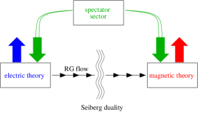
Figure 1: On the left, the schematic set-up for Seiberg duality (and ISS metastability). The blue and red arrows indicate the flavour anomalies generated by the electric and magnetic theories, which may be cancelled by adding a “spectator sector” in the ’t Hooft anomaly matching procedure. On the right, the set-up for holographic metastability. The flavour charges of one sector are conjugated with respect to Seiberg duality so that the gauge anomalies on the IR brane (in red) are now opposite to those of the UV sector (in blue). Both are cancelled by anomaly inflow from a Chern–Simons term in the bulk, which gives equal and opposite contributions to anomalies on the branes.

This is the heuristic picture. Let us now present the model in detail and come back to deal with anomalies and anomaly inflow more carefully in a moment. To mimic the electric and magnetic phases of Seiberg duality, we will use the simple expedient of placing the relevant quarks on their respective branes, but will put some additional meson fields in the bulk. As stated above the latter are uncharged with respect to $\mathrm{SU}(\mathrm{N})$ and $\mathrm{SU}(\mathrm{n})$. The theory is given by Table 3, with the separation into UV brane content, bulk and IR brane content indicated, and depicted once more in Figure 2. As well as the nonabelian symmetries already mentioned, there are two additional abelian symmetries of relevance to us, $\mathrm{U(1)}_{B}$ and $\mathrm{U(1)}_{R}$, both of which are global. As promised, although the assignment superficially resembles that of Seiberg duality in Tables 1 and 2, the $\mathrm{SU(F})_{L}\times\mathrm{SU(F})_{R}\times\mathrm{U(1)}_{B}$ charges (i.e. everything that would be termed a flavour charge in standard Seiberg duality) are reversed.

	$G$	$\mathrm{SU(F})_{L}$	$\mathrm{SU(F})_{R}$	$\mathrm{U}(1)_{B}$	$\mathrm{U}(1)_{R}$
$Q$	$\Box$	$\Box$	1	$\frac{1}{\mathrm{N}}$	$1-\frac{\mathrm{N}}{{\mathrm{F}}}$
$\tilde{Q}$	$\overline{\Box}$	1	$\overline{\Box}$	$-\frac{1}{\mathrm{N}}$	$1-\frac{\mathrm{N}}{{\mathrm{F}}}$
$\Phi$	1	$\overline{\Box}$	$\Box$	0	$-2\frac{\mathrm{N}\mathrm{n}}{{\mathrm{F}}^{2}}$
$\Phi^{c}$	1	$\Box$	$\overline{\Box}$	0	$2+2\frac{\mathrm{N}\mathrm{n}}{{\mathrm{F}}^{2}}$
$\eta$	1	$\Box$	$\overline{\Box}$	0	$2\frac{\mathrm{N}}{{\mathrm{F}}}$
$\eta^{c}$	1	$\overline{\Box}$	$\Box$	0	$2\frac{\mathrm{n}}{{\mathrm{F}}}$
$q$	$\Box$	$\Box$	1	$-\frac{1}{\mathrm{n}}$	$1-\frac{\mathrm{n}}{{\mathrm{F}}}$
$\tilde{q}$	$\overline{\Box}$	1	$\overline{\Box}$	$\frac{1}{\mathrm{n}}$	$1-\frac{\mathrm{n}}{{\mathrm{F}}}$
$\varphi$	1	$\overline{\Box}$	$\Box$	$0$	$2\frac{\mathrm{n}}{{\mathrm{F}}}$

Table 3: Spectrum and anomaly free (with respect to the gauge groups) baryon and R-charges on the UV brane, in the bulk, and on the IR brane. The gauge group $G$ refers to the $\mathrm{SU(N)}$ factor in $\mathrm{SU(n)}\times\mathrm{SU(N)}$ on the UV brane, to the $\mathrm{SU(n)}$ factor on the IR brane.

Figure 2: The field content of the model. The $\mathrm{SU}(\mathrm{\breve{F}}=\mathrm{N}+\mathrm{n})$ bulk gauge group is broken to $\mathrm{SU}(\mathrm{n})\times\mathrm{SU}(\mathrm{N})$ on the branes. On the UV brane the “electric quarks” $Q,\tilde{Q}$ transform only under $\mathrm{SU}(\mathrm{N})$ and are singlets under $\mathrm{SU}(\mathrm{n})$. The opposite is true for the “magnetic quarks” $q,\tilde{q}$ on the IR brane. There are gauge singlets $\Phi$ and $\eta$ in the bulk, and $\varphi$ on the IR brane. In addition there is a weakly gauged $\mathrm{SU}({\mathrm{F}})_{L}\times\mathrm{SU}({\mathrm{F}})_{R}$ flavour symmetry.

The bulk fields $\eta$ and $\eta^{c}$ are conjugate pairs of $D=4$, $\mathcal{N}=1$ superfields which together constitute a 5D hypermultiplet. We take $\eta$ to be even and $\eta^{c}$ to be odd under both orbifold projections. The 5D action reads [27, 26, 28]

$$\begin{split}{\cal S}\leavevmode\nobreak\ =\leavevmode\nobreak\ &\int d^{5}x\Bigl{\{}\int d^{4}\theta\,e^{-2ky}\,\left[\eta e^{-V}\eta^{\dagger}+\eta^{c}e^{V}\eta^{c\dagger}\right]\\ &+\int d^{2}\theta e^{-3ky}\,\Bigl{[}\eta^{c}\left(\mathcal{D}_{y}-\left(\frac{3}{2}-c_{\eta}\right)k\right)\eta+\delta(y)W_{\mbox{\tiny UV}}+\delta(y-\pi R)e^{-3ky}W_{\mbox{\tiny IR}}\Bigr{]}+{\rm h.c.}\Bigr{\}}\end{split}$$ (16)

where $\mathcal{D}$ is the covariant derivative and where $c_{\eta}$ leads to a bulk Dirac mass. We assume that no components of the gauge fields get vevs, so we may for this discussion set $\mathcal{D}_{y}\equiv\partial_{y}$. Since the brane superpotentials $W_{\mbox{\tiny UV}}$ and $W_{\mbox{\tiny IR}}$ cannot depend on the odd fields $\eta^{c}$, the $F$-term equations are

$$e^{-2ky}F^{\dagger}_{\eta} = e^{-3ky}\left(\partial_{y}-\left(\frac{3}{2}+c_{\eta}\right)k\right)\eta^{c}-\delta(y)\partial_{\eta}W_{\mbox{\tiny UV}}-\delta(y-\pi R)e^{-3k\pi R}\partial_{\eta}W_{\mbox{\tiny IR}}\,,$$

$$e^{-2ky}F^{\dagger}_{\eta^{c}} = e^{-3ky}\left(-\partial_{y}+\left(\frac{3}{2}-c_{\eta}\right)k\right)\eta\,.$$ (17)

The bulk solution for $\eta$ is of the form

$$\eta=A\,e^{(\frac{3}{2}-c_{\eta})k|y|}.$$ (18)

The normalized modes are $\hat{\eta}=e^{-ky}\eta$, so that if $c_{\eta}>1/2$ we have localization around $y=0$ whereas $c_{\eta}<1/2$ gives localization around $y=\pi R$. These general solutions have to be matched to whatever vev $\eta$ may acquire due to brane interaction terms. The discussion for the other pair of bulk fields, $\Phi$ and $\Phi^{c}$, is entirely analogous.

The charges and global symmetries do not allow a superpotential on the UV brane (i.e. $W_{\mbox{\tiny UV}}=0$), but they do allow arbitrary Dirac masses in the bulk, and an IR superpotential of

$$e^{-{3k\pi R}}W_{\mbox{\tiny IR}}=h\,(q\varphi\tilde{q})+\mu_{\mbox{\tiny IR}}\,(\hat{\eta}\varphi)\,.$$ (19)

where $\mu_{\mbox{\tiny IR}}\sim e^{-k\pi R}\mu_{\mbox{\tiny UV}}$. (Note that $q$, $\tilde{q}$, $\varphi$ and $\hat{\eta}$ are all defined to be the canonically normalized 4D fields.)

Finally in order to break the gauge group itself (without an adjoint Higgs) we can give boundary conditions of

$$V=\left(\begin{array}[]{c|c}++&+-\\ \hline\cr+-&++\end{array}\right)\,\,;\,\,\Sigma=\left(\begin{array}[]{c|c}--&-+\\ \hline\cr-+&--\end{array}\right),$$ (20)

to the 4D vector and 4D chiral components of the 5D vector supermultiplet, where the blocks refer to $\mathrm{SU}(\mathrm{N})$ and $\mathrm{SU}(\mathrm{n})$ gauge groups. Note that there are no remaining $\Sigma$ zero modes.

3.1 Anomalies and anomaly inflow

In order consistently to gauge the flavour symmetries $\mathrm{SU(F})_{L}$ and $\mathrm{SU(F})_{R}$, they should be anomaly free. Since anomalies are due to fermion zero modes, which are localized in different regions of the internal space in our model, we briefly return to the issue of how local anomaly cancellation can be guaranteed. First we should say that it is well-known that anomaly cancellation in the 4D effective theory is sufficient for cancelling any gauge anomalies in the 5D theory by a suitable bulk Chern–Simons term [29, 30, 31, 32]. We will now briefly describe how this works in our case.

In five non-compact dimensions there is no anomalous divergence of a classically conserved current, as there are no chiral fermions. By locality, anomalies on orbifolds can then only appear on the branes. Both brane-localized fermions and bulk fermion zero modes can contribute. We define the sourceless generating functional $W[A]$ by

$$e^{iW[A]}=\int{\cal D}\Phi\;e^{iS[A,\Phi]},$$ (21)

where the path integral is over all fields $\Phi$ except the gauge field $A$. The anomalous divergence of the gauge current,

$${\cal A}^{a}=(D_{M}J^{M})^{a},$$ (22)

(with the derivative understood to be both gauge-covariant and gravitationally covariant) is then given by the gauge variation of $W$ as

$$\delta_{\alpha}W[A]=\int d^{4}x\int dy\,\sqrt{-g}\,\alpha^{a}\,{\cal A}^{a}.$$ (23)

Since the anomaly is supported only on the branes, we can write

$$\sqrt{-g}\,{\cal A}^{a}(x,y)={\cal A}^{a}_{1}(x)\,\delta(y)+{\cal A}^{a}_{2}(x)\,\delta(y-\pi R).$$ (24)

The ${\cal A}^{a}_{i}(x)$ are determined, up to normalization, by the Wess-Zumino consistency condition. More precisely, they should be proportional to the usual 4D consistent anomaly:

$${\cal A}^{a}_{i}=\frac{n_{i}}{24\pi^{2}}\varepsilon^{\mu\nu\kappa\lambda}\operatorname{tr}\left[T^{a}\,\partial_{\mu}\left(A_{\nu}\partial_{\kappa}A_{\lambda}+\frac{1}{2}A_{\nu}A_{\kappa}A_{\lambda}\right)\right].$$ (25)

Here the gauge fields on the RHS are restricted to the respective branes (hence we can identify them with their 4D zero modes, up to a common normalization, since their bulk profiles are flat). The constants $n_{i}$ depend on the number and distribution of the chiral fermions. Normalizing the trace in Eq. (25) to the fundamental representation, a left-chiral fundamental fermion localized on the $y=0$ ($y=\pi R$) brane will contribute $n_{1}=1,n_{2}=0$ ($n_{1}=0,n_{2}=1$). The contribution from a massless left-chiral bulk fermion is $n_{1}=n_{2}=1/2$. On the $S^{1}/(Z_{2}\times Z_{2}^{\prime})$ orbifold which we are considering, fermions with orbifold parities $(+-)$ and $(-+)$ may also contribute to localized anomalies (even though they do not give rise to 4D zero modes). The contribution from a fundamental fermion with parity $(+-)$ is $n_{1}=-n_{2}=1/2$; from a fermion with parity $(-+)$, it is $n_{1}=-n_{2}=-1/2$. Note that, by the topological nature of the anomaly, the warp factor never enters here and the discussion is similar to the flat case.

For the 4D effective theory, obtained by integrating over $y$, to be anomaly-free, it is necessary and sufficient for ${\cal A}_{1}$ and ${\cal A}_{2}$ to be equal and opposite. If ${\cal A}_{1}=-{\cal A}_{2}$ and both are nonzero, the 5D theory still appears anomalous on the branes. In that case, in order to render the theory consistent, the anomalous gauge variation of the generating functional should be compensated by a 5D Chern–Simons term

$${\cal L}_{\rm CS}=\frac{c}{96\pi^{2}}\,\varepsilon^{MNOPQ}\operatorname{tr}\left[A_{M}F_{NO}F_{PQ}+i\,A_{M}A_{N}A_{O}F_{PQ}-\frac{2}{5}A_{M}A_{N}A_{O}A_{P}A_{Q}\right].$$ (26)

The gauge variation of the Chern–Simons term is a total divergence, leading to equal and opposite boundary terms on the branes that may precisely cancel the anomaly of Eq. (25) for suitable $c$. This is the “anomaly inflow” mechanism [33].

As an example consider the $\mathrm{SU(F})_{L}$ flavour group of the model in Table 3. There are $\mathrm{N}$ fundamentals $Q$ on the $y=0$ brane, ${\mathrm{F}}$ fundamentals $\eta$ and ${\mathrm{F}}$ antifundamentals $\Phi$ in the bulk (note that $\Phi^{c}$ and $\eta^{c}$ do not contribute since they have parities $(--)$), and $\mathrm{n}$ fundamentals $q$ as well as ${\mathrm{F}}$ antifundamentals $\varphi$ on the $y=\pi R$ brane. The anomalies due to bulk fields cancel; the remaining anomaly is

$${\cal A}^{a}_{\mathrm{SU(F})_{L}}=\frac{\mathrm{N}}{24\pi^{2}}\varepsilon^{\mu\nu\kappa\lambda}\operatorname{tr}\left[T^{a}\,\partial_{\mu}\left(A_{\nu}\partial_{\kappa}A_{\lambda}+\frac{1}{2}A_{\nu}A_{\kappa}A_{\lambda}\right)\right]\;\left[\delta(y)-\delta(y-\pi R)\right]\,e^{4ky}\,.$$ (27)

It is cancelled by a bulk Chern–Simons term

$${\cal L}_{\rm CS}=\frac{\mathrm{N}}{192\pi^{2}}\,\varepsilon^{MNOPQ}\operatorname{tr}\left[A_{M}F_{NO}F_{PQ}+i\,A_{M}A_{N}A_{O}F_{PQ}-\frac{2}{5}A_{M}A_{N}A_{O}A_{P}A_{Q}\right].$$ (28)

From a 4D viewpoint one can therefore simply add the contributions of the zero-modes: the $\mathrm{SU(F})_{L}^{3}$ anomaly on the UV brane is $\mathrm{N}$, and on the IR brane is $\mathrm{n}-{\mathrm{F}}=-\mathrm{N}$, and there is no nett anomaly contribution from the zero modes of the even bulk fields. Summarizing the remaining anomalies, the $\mathrm{U(1)}_{R}$ charges in Table 3 are fixed by the vanishing of the $G^{2}-\mathrm{U(1)}_{R}$ anomalies (which implies $R_{\eta}+R_{\Phi}=2\frac{\mathrm{N}^{2}}{{\mathrm{F}}^{2}}$) and by the $\varphi q\tilde{q}$ and $\eta\varphi$ couplings in the IR superpotentials. The $\mathrm{U(1)}_{B}$ charges are fixed by the $\mathrm{SU(F})^{2}-\mathrm{U(1)}_{B}$ anomalies. The gauge group $\mathrm{n}={\mathrm{F}}-\mathrm{N}$ is fixed by the $\mathrm{SU(F})^{3}$ anomalies. Note that $\mathrm{U(1)}_{B}$ and $\mathrm{U(1)}_{R}$ are global and there remain uncancelled $\mathrm{U(1)}_{R}^{3}$ and $\mathrm{U(1)}_{R}-\mathrm{U(1)}_{B}^{2}$ anomalies, but these symmetries are indeed anomaly free with respect to the gauge symmetries as required.

3.2 Baryon matching

To complete this section we briefly demonstrate another equivalence that can be drawn between the holographic picture outlined here and that of standard Seiberg duality, namely the identification of baryons. In Seiberg duality one of the major tests of the equivalence of the electric and magnetic formulations is that the moduli spaces match: in particular there exists a precise mapping between magnetic and electric baryons. Returning to the SQCD content of Tables 1 and 2 for a moment, this mapping is of the form

$$\varepsilon^{({\mathrm{F}})}\varepsilon^{(\mathrm{N})}Q^{\mathrm{N}}\equiv\varepsilon^{(\mathrm{n})}q^{\mathrm{n}},$$ (29)

where the $\varepsilon^{({\mathrm{F}})}$ Levi-Cevita symbol refers to a contraction over “flavour” indices (and similar for antibaryons). Note that the $\varepsilon^{({\mathrm{F}})}$ yields an object on the LHS that transforms with ${\mathrm{F}}-\mathrm{N}=\mathrm{n}$ antisymmetric flavour indices, exactly matching the RHS. Indeed this contraction is why the flavour charges on the quarks have to be negated in the magnetic theory (i.e. the electric quarks are flavour fundamentals whereas the magnetic ones are flavour antifundamentals). The baryons can be labelled as follows

$$\varepsilon^{({\mathrm{F}})}B\equiv b$$ (30)

where $B=\varepsilon^{(\mathrm{N})}Q^{\mathrm{N}}$ and $b=\varepsilon^{(\mathrm{n})}q^{\mathrm{n}}$ have respectively $\mathrm{N}$ and $\mathrm{n}$ antisymmetric flavour indices. Now let us return to the AdS model and consider the bulk $\mathrm{SU}(\mathrm{\breve{F}})$ symmetry. Clearly the $\mathrm{SU(N)}$ and $\mathrm{SU(n)}$ quarks fit into full $\mathrm{SU}(\mathrm{\breve{F}})$ fundamentals so that the quark content in the unbroken theory would be as shown in Table 4.

	$\mathrm{SU}(\mathrm{\breve{F}})$	$\mathrm{SU(F})_{L}$	$\mathrm{SU(F})_{R}$	$\widetilde{\mathrm{U}}(1)_{B}$	$\widetilde{\mathrm{U}}(1)_{R}$
$\mathbf{Q}\supset Q,\,q$	$\Box$	$\Box$	1	$\frac{1}{\mathrm{\breve{F}}}$	$0$
$\mathbf{\tilde{Q}}\supset\tilde{Q},\,\tilde{q}$	$\overline{\Box}$	$1$	$\overline{\Box}$	$-\frac{1}{\mathrm{\breve{F}}}$	$0$

Table 4: Quarks in the unified $\mathrm{SU}(\mathrm{\breve{F}})$ theory.

The baryons in the unbroken theory would be

$$\mathbf{B}=\varepsilon^{(\mathrm{\breve{F}})}\mathbf{Q}^{{\mathrm{F}}},$$ (31)

with $\mathrm{\breve{F}}$ flavour indices. Thus (upto permutation factors) the singlet object is

$$\varepsilon^{({\mathrm{F}})}\mathbf{B} = \varepsilon^{({\mathrm{F}})}\varepsilon^{(\mathrm{N})}\varepsilon^{(\mathrm{n})}Q^{\mathrm{N}}q^{\mathrm{n}}$$ (32)

$$= \varepsilon^{({\mathrm{F}})}B\,b.$$

This allows us to identify each $B$ with an $\mathrm{SU(n)}$ antiquark:

$$\varepsilon^{({\mathrm{F}})}B\equiv\tilde{b}.$$ (33)

As one might expect the identification is simply the conjugate of that in Seiberg duality in eq.(30), and indeed the magnetic “baryon” $b=q^{\mathrm{n}}$ carries baryon charge $-1$.

4 Supersymmetry breaking

Let us now now turn to the question of SUSY breaking. The IR superpotential of (19) is similar to that of ISS, but with the linear term replaced by a brane mass term $\mu_{\mbox{\tiny IR}}\,\hat{\eta}\varphi$. Clearly what is required for SUSY breaking is a vev for $\eta$. Following the thinking outlined in the introduction, we wish to achieve this by a deformation of the UV theory. Hence we break the global $R$-symmetry in the UV theory with terms allowed by the other symmetries,

$$W_{\mbox{\tiny UV}}=\mu_{\mbox{\tiny UV}}\eta\Phi-\frac{1}{2}\frac{\eta\Phi\eta\Phi}{\mu_{\mbox{\tiny UV}}}\,.$$ (34)

A good approximation is to first consider unbroken SUSY on the UV brane. These terms can then generate vevs for both $\eta$ and $\Phi$ as can be seen by setting the $F$-terms equal to zero. By a choice of gauge they can be chosen to be diagonal, and then the $D$-term contribution to the potential sets $\eta=\Phi=\mu_{\mbox{\tiny UV}}\mathbbm{1}$ in the vacuum with maximal remaining symmetry. (Note that the mesons are effectively ${\mathrm{F}}$ generations of fundamental or antifundamental with respect to a particular $\mathrm{SU(F})_{L}$ or $\mathrm{SU(F})_{R}$.) In this way the flavour symmetry can be broken down to the diagonal symmetry $\mathrm{SU(F})_{L}\times\mathrm{SU(F})_{R}\rightarrow\mathrm{SU(F})_{D}$ as in ISS. We may also add a

$$W_{\mbox{\tiny UV}}\supset Q\Phi\tilde{Q}$$

coupling. Once $\Phi$ gets a vev, this term generates precisely the $m_{Q}$ deformation, but with an unsuppressed mass, $m_{Q}\sim\mu_{\mbox{\tiny UV}}$.

It is reasonable to assume that some spontaneous breaking of $R$-symmetry in the fundamental UV theory generates these terms. The mass term can be generated by some $R$-charged singlet fields getting a vev for example, or both it and the quartic term may be generated by gravitational effects since the $R$-symmetry is after all only global. Note here a marked departure from the ISS model: the $R$-symmetry breaking that subsequently appears in the IR theory is under rigid control. Indeed according to (18) the vev of $\hat{\eta}$ is

$$\hat{\eta}=\mu_{\mbox{\tiny UV}}\,e^{(\frac{1}{2}-c_{\eta})ky},$$ (35)

so that the effective superpotential (19) becomes the O’Raifeartaigh/ISS one:

$$W_{\mbox{\tiny IR}}=h\,q\varphi\tilde{q}+\mu_{\mbox{\tiny ISS}^{\prime}}^{2}\varphi\,.$$ (36)

where

$$\mu_{\mbox{\tiny ISS}^{\prime}}^{2}=e^{-\left(\frac{1}{2}+c_{\eta}\right)k\pi R}\mu_{\mbox{\tiny UV}}^{2}.$$ (37)

Note that a warped down mass-squared term would be of order $e^{-2k\pi R}\mu_{\mbox{\tiny UV}}^{2}$. For $c_{\eta}=1/2$ the parameter $\mu_{\mbox{\tiny ISS}^{\prime}}$ scales with a single power of the warp factor because the wave-function of $\hat{\eta}$ is evenly spread over the compact dimension. By taking $c_{\eta}>1/2$ one makes $\mu_{\mbox{\tiny ISS}^{\prime}}$ further exponentially suppressed, due to the localization of the zero-mode of $\hat{\eta}$ on the UV brane.

Hence the IR theory develops a metastable minimum as in ISS [7], and as in ISS it has a remaining anomalous $R$-symmetry responsible for the supersymmetric minima being situated at large $\varphi$ vev. In order for the 4D description to be trustable however there are additional constraints on the parameter $c_{\eta}$. Since the metastable minimum has quark vevs of order $\mu_{\mbox{\tiny ISS}^{\prime}}$, and the KK modes of the theory have masses of order $\mu_{\mbox{\tiny IR}}=e^{-k\pi R}\mu_{\mbox{\tiny UV}}$, we have a necessary condition,

$$\mu_{\mbox{\tiny ISS}^{\prime}}<\mu_{\mbox{\tiny IR}}\,.$$ (38)

This enforces

$$c_{\eta}>\frac{3}{2}\,.$$ (39)

Additional constraints arise if one requires the global SUSY minimum (and hence aspects of the metastability such as the tunnelling rate) to be well under control entirely within the low energy 4D description. A sufficient condition for this would be that the $\varphi$ vev (11) is less than the KK mode scale $\mu_{\mbox{\tiny IR}}$. This depends on the choice of dynamical transmutation scale $\bar{\Lambda}$ in the IR theory. In order to have perturbative control this should certainly be greater than $\mu_{\mbox{\tiny IR}}$. In the limiting case that $\bar{\Lambda}\sim\mu_{\mbox{\tiny IR}}$ we find the same necessary condition $\mu_{\mbox{\tiny ISS}^{\prime}}<\mu_{\mbox{\tiny IR}}$, and hence $c_{\eta}>\frac{3}{2}$, for the SUSY restoring vacuum to be visible within the 4D theory. The general necessary condition that includes a valid metastable minimum, and a global supersymmetric minimum much further from the origin but less than $\mu_{\mbox{\tiny IR}}$ is

$$\mu_{\mbox{\tiny ISS}^{\prime}}\ll\langle\varphi\rangle\sim\mu_{\mbox{\tiny ISS}^{\prime}}\epsilon^{\alpha}\sim\bar{\Lambda}\epsilon^{\alpha+1}<\mu_{\mbox{\tiny IR}}\ll\bar{\Lambda}\,,$$ (40)

where $\alpha=\frac{2F-3N}{N}$ and as before $\epsilon=\mu_{\mbox{\tiny ISS}^{\prime}}/\bar{\Lambda}$. This requires $\alpha$ to be in the range $0>\alpha>-1$, so that for small enough $\epsilon$ one can always achieve $\mu_{\mbox{\tiny ISS}^{\prime}}\ll\langle h\varphi\rangle\ll\bar{\Lambda}$. In terms of numbers of colours and flavours this becomes

$$\frac{3N}{2}>F>N,$$ (41)

precisely the requirement in the ISS model that one is in the free magnetic phase. (Of course $F>N$ is satisfied in this model by design.)

Since we break $R$ symmetry in the UV, $R$-symmmetry breaking operators on the IR brane will generically be induced, and they will lead to additional supersymmetric vacua. It is, however, readily checked that these are far away in field space and thus not dangerous. First, note that a $\varphi^{2}$ term cannot be induced even though the remaining symmetry $\mathrm{SU(F})_{D}$ allows it, because the $\mathrm{SU(F})_{L}\times\mathrm{SU(F})_{R}\rightarrow\mathrm{SU(F})_{D}$ breaking is spontaneous and proportional to $\langle\eta\rangle$. Also, since the possible operators would be generated in the UV theory (by gravity for example) one would expect them always to be suppressed by powers of $\mu_{\mbox{\tiny UV}}$. (Even if they are absent in the superpotential, there can be similarly suppressed operators in the Kähler potential.) In this case one can have for instance, a term

$$W_{\mbox{\tiny IR}}\leavevmode\nobreak\ \supset\leavevmode\nobreak\ \frac{(\varphi\hat{\eta})^{2}}{\mu_{\mbox{\tiny UV}}}$$ (42)

which would in principle induce a minimum at

$$\langle\varphi\rangle\sim\frac{\mu_{\mbox{\tiny IR}}\mu_{\mbox{\tiny UV}}}{\langle\hat{\eta}\rangle}\sim\frac{\mu_{\mbox{\tiny IR}}^{2}\mu_{\mbox{\tiny UV}}}{(\mu_{\mbox{\tiny ISS}^{\prime}})^{2}}\gg\mu_{\mbox{\tiny IR}}\,.$$ (43)

However, since $\mu_{\mbox{\tiny ISS}^{\prime}}\ll\mu_{\mbox{\tiny IR}}$ and $\mu_{\mbox{\tiny UV}}\gg\mu_{\mbox{\tiny IR}}$ this lies outside the region of validity of the IR theory and it cannot destabilize the metastable minimum. (To be very conservative, even if one were to consider the lowest possible suppression scale of $\mu_{\mbox{\tiny IR}}$ in Eq. (42), the global SUSY restoring minima would still be still sufficiently far away.)

An (appropriately suppressed) IR brane operator of the form $q\Phi\tilde{q}$ could be useful if we identify (part of) the magnetic quarks as messenger fields for gauge mediation. It would effectively be a mass term for $q$ and $\tilde{q}$; since their vevs leave an $\mathrm{SU(N)}$ subgroup of the $\mathrm{SU(F})_{D}$ flavour group unbroken, one could imagine identifying this subgroup with the visible sector gauge group. Soft masses would then be generated, as usual in gauge mediation, by $q$ and $\tilde{q}$ loops.

As a final remark, in the metastable SUSY breaking vacuum the expectation value of the bulk fields $\eta$ and $\Phi$ (which we determined in a first approximation from the condition for unbroken SUSY) will receive small corrections because the potential is now elevated by an additional term $\sim\mathrm{N}|h\mu_{\mbox{\tiny ISS}^{\prime}}^{2}|^{2}$. These corrections are suppressed by the warping (i.e. they are a correction of order $e^{-2\pi kR}\mu_{\mbox{\tiny UV}}$ in the vev of $\eta$ on the UV brane), so they can be consistently neglected for our analysis.

4.1 Holographic interpretation

By the AdS/CFT correspondence [13, 14, 15], an RS1 type model on a “slice of AdS₅” can be regarded as dual to a 4D conformal field theory. The AdS/CFT dictionary relates the building blocks of the 5D theory to objects on the CFT side [34, 35]. Specifically, the fifth dimension $y$ of AdS₅ becomes the renormalization scale in the CFT; the truncation of AdS₅ at $y=0$ by a UV brane corresponds to introducing a UV cutoff scale for the CFT, coupling it to gravity and possibly other fundamental degrees of freedom; and the truncation at $y=\pi R$ by an IR brane corresponds to a spontaneous breaking of conformal invariance in the infra-red. The CFT is strongly coupled, because gravity on the AdS side is weakly coupled (gravitational dynamics is, of course, completely negligible for our analysis). Bulk gauge groups in AdS correspond to internal global symmetries of the CFT which are weakly gauged, so as not to affect the CFT dynamics. Localized fields on the UV brane correspond to fundamental, “elementary” fields external to the CFT, while localized fields on the IR brane are interpreted as “composite” bound states formed by the CFT degrees of freedom. Fields propagating in the 5D bulk should be regarded as being partly composite and partly elementary.

It is interesting to see how the 4D CFT interpretation of our model relates to a purely four-dimensional, conventional ISS model retrofitted by an additional, strongly coupled gauge sector. Clearly some aspects are analogous: for instance, by construction the far infra-red dynamics is more or less the same. That is, in the 4D effective theory of our model we can integrate out the $\eta$ as well as $\Phi$ and the electric quarks at scales below $m_{Q}$, $\mu_{\mbox{\tiny UV}}$. Then we are left with only the IR brane degrees of freedom, constituting the magnetic side of an ISS model, and a pure $\mathrm{SU(N)}$ gauge theory which is effectively decoupled.

Similarly, the purely elementary degrees of freedom are, according to the AdS/CFT dictionary, just those living on the UV brane. In our case these are just the electric quarks, which together with the $\mathrm{SU(N)}$ gauge fields form the corresponding Seiberg dual electric theory.

In an ISS model, one may think of the small electric quark mass (which is eventually responsible for dynamical SUSY breaking) as being generated by strong dynamics of an additional gauge sector (see e.g. [19, 20, 23, 24]). Our model is similar in the sense that the meson mass term in the magnetic theory is naturally small, because it is suppressed by the warp factor and by the $\eta$ bulk profile in the AdS picture. In the CFT picture the reason for its suppression is that it is again generated dynamically.

There is, however, an important difference in that strong coupling of the bulk gauge group never plays a role in our model. This is very much in contrast to the usual 4D picture of Seiberg duality, where the electric gauge group has a Landau pole around the same scale as the magnetic gauge group, defining where the transition between electric and magnetic degrees of freedom takes place. In fact, in our model we are delaying the onset of strong coupling for both the magnetic and the electric gauge factors beyond the range of validity of a purely magnetic or electric description. That is, the $\mathrm{SU(n)}$ and $\mathrm{SU(N)}$ gauge couplings should unify near the compactification scale into the $\mathrm{SU}(\mathrm{\breve{F}})$ gauge coupling, which should be perturbative at that scale. Formally the magnetic sector has a Landau pole in the UV, which is however at a much higher scale where the description in terms of far IR degrees of freedom is no longer valid. Likewise, the electric sector would become strongly coupled in the infra-red if the quark mass was sufficiently small. However, since $m_{Q}\sim\mu_{\mbox{\tiny UV}}$ is large the electric quarks decouple before strong coupling is reached. What remains of the electric theory is then a pure SYM theory which couples to the magnetic sector only through irrelevant operators.

Acknowledgements

We are grateful to Tony Gherghetta for very useful conversations. SAA acknowledges a Leverhulme Research Fellowship.

References

- [1] E. Witten, “Dynamical Breaking Of Supersymmetry,” Nucl. Phys. B 188, 513 (1981).
- [2] I. Affleck, M. Dine and N. Seiberg, “Supersymmetry Breaking By Instantons,” Phys. Rev. Lett. 51, 1026 (1983).
- [3] I. Affleck, M. Dine and N. Seiberg, “Dynamical Supersymmetry Breaking In Supersymmetric QCD,” Nucl. Phys. B 241, 493 (1984).
- [4] I. Affleck, M. Dine and N. Seiberg, “Dynamical Supersymmetry Breaking In Four-Dimensions And Its Phenomenological Implications,” Nucl. Phys. B 256, 557 (1985).
- [5] N. Seiberg, “Electric-magnetic duality in supersymmetric non-abelian gauge theories", Nucl. Phys. B 435(1), 129–146 (1995), [arXiv:hep-th/9411149].
- [6] For a review see K. A. Intriligator and N. Seiberg, “Lectures on supersymmetric gauge theories and electric-magnetic duality,” Nucl. Phys. Proc. Suppl. 45BC, 1 (1996) [arXiv:hep-th/9509066].
- [7] K. A. Intriligator, N. Seiberg and D. Shih, “Dynamical SUSY breaking in meta-stable vacua,” JHEP 0604 (2006) 021 [arXiv:hep-th/0602239].
- [8] J. R. Ellis, C. H. Llewellyn Smith and G. G. Ross, “Will The Universe Become Supersymmetric?,” Phys. Lett. B 114, 227 (1982).
- [9] M. Dine, A. E. Nelson, Y. Nir and Y. Shirman, “New tools for low-energy dynamical supersymmetry breaking,” Phys. Rev. D 53, 2658 (1996) [arXiv:hep-ph/9507378].
- [10] S. Dimopoulos, G. R. Dvali, R. Rattazzi and G. F. Giudice, “Dynamical soft terms with unbroken supersymmetry,” Nucl. Phys. B 510, 12 (1998) [arXiv:hep-ph/9705307].
- [11] M. A. Luty and J. Terning, “Improved single sector supersymmetry breaking,” Phys. Rev. D 62, 075006 (2000) [arXiv:hep-ph/9812290].
- [12] T. Banks, “Cosmological supersymmetry breaking and the power of the pentagon: A model of low energy particle physics,” arXiv:hep-ph/0510159.
- [13] J. M. Maldacena, “The large N limit of superconformal field theories and supergravity,” Adv. Theor. Math. Phys. 2, 231 (1998) [Int. J. Theor. Phys. 38, 1113 (1999)] [arXiv:hep-th/9711200].
- [14] S. S. Gubser, I. R. Klebanov and A. M. Polyakov, “Gauge theory correlators from non-critical string theory,” Phys. Lett. B 428 (1998) 105 [arXiv:hep-th/9802109].
- [15] E. Witten, “Anti-de Sitter space and holography,” Adv. Theor. Math. Phys. 2 (1998) 253 [arXiv:hep-th/9802150].
- [16] A. E. Nelson and N. Seiberg, “R symmetry breaking versus supersymmetry breaking,” Nucl. Phys. B 416, 46 (1994) [arXiv:hep-ph/9309299].
- [17] E. Dudas, J. Mourad and F. Nitti, “Metastable Vacua in Brane Worlds,” JHEP 0708, 057 (2007) [arXiv:0706.1269 [hep-th]].
- [18] H. Abe, T. Kobayashi and Y. Omura, “Metastable supersymmetry breaking vacua from conformal dynamics,” Phys. Rev. D 77, 065001 (2008) [arXiv:0712.2519 [hep-ph]].
- [19] M. Dine, J. L. Feng and E. Silverstein, “Retrofitting O’Raifeartaigh models with dynamical scales,” Phys. Rev. D 74, 095012 (2006) [arXiv:hep-th/0608159].
- [20] M. Dine and J. Mason, “Gauge mediation in metastable vacua,” Phys. Rev. D 77, 016005 (2008) [arXiv:hep-ph/0611312].
- [21] S. A. Abel, C. Durnford, J. Jaeckel and V. V. Khoze, “Patterns of Gauge Mediation in Metastable SUSY Breaking,” JHEP 0802, 074 (2008) [arXiv:0712.1812 [hep-ph]].
- [22] H. Murayama and Y. Nomura, “Gauge mediation simplified,” Phys. Rev. Lett. 98, 151803 (2007) [arXiv:hep-ph/0612186].
- [23] O. Aharony and N. Seiberg, “Naturalized and simplified gauge mediation,” JHEP 0702, 054 (2007) [arXiv:hep-ph/0612308].
- [24] F. Brümmer, “A natural renormalizable model of metastable SUSY breaking,” JHEP 0707 (2007) 043 [arXiv:0705.2153 [hep-ph]].
- [25] L. Randall and R. Sundrum, “A large mass hierarchy from a small extra dimension,” Phys. Rev. Lett. 83 (1999) 3370 [arXiv:hep-ph/9905221].
- [26] D. Marti and A. Pomarol, “Supersymmetric theories with compact extra dimensions in N = 1 superfields,” Phys. Rev. D 64, 105025 (2001) [arXiv:hep-th/0106256].
- [27] T. Gherghetta and A. Pomarol, “Bulk fields and supersymmetry in a slice of AdS,” Nucl. Phys. B 586 (2000) 141 [arXiv:hep-ph/0003129].
- [28] T. Gherghetta, “Warped models and holography,” arXiv:hep-ph/0601213.
- [29] N. Arkani-Hamed, A. G. Cohen and H. Georgi, “Anomalies on orbifolds,” Phys. Lett. B 516, 395 (2001) [arXiv:hep-th/0103135].
- [30] C. A. Scrucca, M. Serone, L. Silvestrini and F. Zwirner, “Anomalies in orbifold field theories,” Phys. Lett. B 525 (2002) 169 [arXiv:hep-th/0110073].
- [31] R. Barbieri, R. Contino, P. Creminelli, R. Rattazzi and C. A. Scrucca, “Anomalies, Fayet-Iliopoulos terms and the consistency of orbifold field theories,” Phys. Rev. D 66, 024025 (2002) [arXiv:hep-th/0203039].
- [32] S. Groot Nibbelink, H. P. Nilles and M. Olechowski, “Instabilities of bulk fields and anomalies on orbifolds,” Nucl. Phys. B 640 (2002) 171 [arXiv:hep-th/0205012].
- [33] C. G. . Callan and J. A. Harvey, “Anomalies And Fermion Zero Modes On Strings And Domain Walls,” Nucl. Phys. B 250 (1985) 427.
- [34] N. Arkani-Hamed, M. Porrati and L. Randall, “Holography and phenomenology,” JHEP 0108 (2001) 017 [arXiv:hep-th/0012148].
- [35] R. Rattazzi and A. Zaffaroni, “Comments on the holographic picture of the Randall-Sundrum model,” JHEP 0104 (2001) 021 [arXiv:hep-th/0012248].