Ultra- and Hyper-compact HII regions at 20 GHz

Abstract

We present radio and infrared observations of 4 hyper-compact HII regions and 4 ultra-compact HII regions in the southern Galactic plane. These objects were selected from a blind survey for UCHII regions using data from two new radio surveys of the southern sky; the Australia Telescope 20 GHz survey (AT20G) and the 2nd epoch Molonglo Galactic Plane Survey (MGPS-2) at 843 MHz. To our knowledge, this is the first blind radio survey for hyper- and ultra-compact HII regions.

We have followed up these sources with the Australia Telescope Compact Array to obtain H$70\alpha$ recombination line measurements, higher resolution images at 20 GHz and flux density measurements at 30, 40 and 95 GHz. From this we have determined sizes and recombination line temperatures as well as modeling the spectral energy distributions to determine emission measures. We have classified the sources as hyper-compact or ultra-compact on the basis of their physical parameters, in comparison with benchmark parameters from the literature.

Several of these bright, compact sources are potential calibrators for the Low Frequency Instrument (30$-$70 GHz) and the 100-GHz channel of the High Frequency Instrument of the Planck satellite mission. They may also be useful as calibrators for the Australia Telescope Compact Array, which lacks good non-variable primary flux calibrators at higher frequencies and in the Galactic plane region. Our spectral energy distributions allow the flux densities within the Planck bands to be determined, although our high frequency observations show that several sources have excess emission at 95 GHz (3 mm) that can not be explained by current models.

1 Introduction

The process of massive star formation is thought to proceed via collapse and accretion from a dense molecular cloud. According to this scenario, a hot molecular gas core evolves to produce a massive star within a dense cocoon of gas and dust, most readily detected at this early stage by infrared and sub-mm emission. As the Lyman continuum from the fledgling star begins to ionize its environs, free-free radio emission is detected and the phase designated as an ultra-compact HII region (UCHII) begins. Wood & Churchwell (1989) first defined this phase observationally and determined that these objects were distinct from more evolved HII regions, which are typically optically thin at radio wavelengths. UCHII regions are very small ($<0.1$ pc), dense ($>10^{4}$ cm^-3) ionized regions of gas that surround the youngest and most massive O and B stars. The lifetime of an UCHII is estimated to be less than 10⁵ years (Comeron & Torra, 1996).

While UCHII regions were thought to be the intermediate stage between a massive star being formed in a hot molecular core and a fully formed compact HII region of ionised gas, it was discovered by Gaume et al. (1995) that there is an even earlier phase just after the star is newly formed, but presumably before it becomes an UCHII region. In this phase the object is called a hyper-compact HII region (HCHII) and is characterised by more extreme parameters, namely electron densities ($n_{e}$) $>10^{6}$ cm^-3, emission measures (EMs) of $>10^{8}$ pc cm^-6 and physical size $<0.05$ pc. These objects typically have broadened radio recombination lines, when compared with the expected line width due to thermal and turbulent broadening found in more evolved HII regions.

Results from Sewilo et al. (2004), Kurtz (2005), and Gaume et al. (1995) show that the HCHII recombination lines range in width from about 40 to 250 km s^-1. These broad lines could be explained by bulk motions of gas (infall, outflow or rotation), pressure broadening or a blending of components. Sewilo et al. (2004) studied seven massive star-forming regions and found eight components with broad recombination lines, potentially indicating HCHII regions. In some sources a double-peaked profile may indicate infalling gas as an ionized accretion flow (Keto, 2003). A halo of diffuse gas, optically thin at 3.6 cm, surrounding the HCHII candidates was a surprise as was the presence of multiple massive stars at the same early evolutionary phase, given their expected brief lifetimes.

Such a precise definition of an HCHII region is somewhat artificial and the question of whether there is merely a continuum in evolutionary phases or whether HCHII represent a distinct class of objects remains unresolved. For example, Kurtz (2005) speculates that HCHII regions are signposts for individual stars, whereas the objects classified as UCHII regions often contain clusters.

The currently identified HCHII regions are heavily optically obscured by a thick cocoon of dust and are very rare, principally for two reasons. Firstly, there is a strong selection bias in the early surveys searching for young HII regions. These surveys, mostly around $\lambda$ 6 cm, were optimised for objects with electron densities about $10^{4}$ cm^-3. At higher densities an object remains optically thick to a much higher frequency and will below the detection limit (Kurtz, 2005). The second constraint is that the expected lifetime of this phase is likely to be brief (Comeron & Torra, 1996) and potentially difficult to capture.

In this early phase of massive stellar evolution, no optical and minimal near-infrared light emerges from the core because of the enormous amount of surrounding dust. Radiative transfer maintains a large gradient in dust temperature from the core to the outer surface of the dust shell and the region emits brightly from the far- to mid-infrared (FIR, MIR) regime. If there is a continuum of evolutionary stages, then as the star ages the HCHII expands, becoming first an UCHII and then a compact HII region, defined as having a size of $<0.5\,\rm{pc}$. Subsequently, the FIR$-$MIR emission fades and eventually the dust becomes optically thin at visible wavelengths and the birth process is complete.

The stellar radiation from the HCHII and UCHII phases is absorbed by the cocoon of molecular gas and dust and re-emitted in the far-infrared. As a result, they are amongst the brightest point sources in the IRAS 100 $\mu$m catalogue. At radio wavelengths the surrounding molecular gas and dust is transparent, and so UCHII regions appear as bright unresolved continuum sources. It is not clear at what stage the HCHII regions become bright radio sources, as they may be optically thick at lower frequencies. The continuum emission is often associated with OH and H₂O masers, which indicates that the UCHII regions are affected by stellar winds, bow shocks, masers and other dynamical processes in star formation regions. Some HCHII regions are also associated with the masers, particularly H₂O masers which are produced by dense gas. For example G75.78$+$0.34 (Hofner & Churchwell, 1996) and NGC 7538 (see summary in Sewilo et al. (2004)).

Although UCHII were initially defined on the basis of being unresolved in radio continuum observations, high resolution ($<1\arcsec$) radio observations have revealed a variety of morphologies. These have been classified into 5 general types by Wood & Churchwell (1989): Spherical (or unresolved), Cometary (parabolic), Core-halo, Shell and Irregular (or multiply peaked). The apparent shape of an UCHII is affected by the optical depth of the gas at the particular observing frequency. When gas is optically thick, only the surface of the UCHII region is visible, and the internal structure is hidden. UCHII usually have an inverted (or rising) spectral index at radio frequencies and are much brighter in the FIR/MIR regime.

The observational morphologies for HCHII regions are less well known. From the literature, we have collated a working definition of HCHII regions as a stage in development earlier than UCHII (see Section 5). The difficulty in determining morphologies is that the sources are largely unresolved. The fit to a simple one component model and its limitations are discussed later in this paper.

The objects presented here are drawn from a complete sample of 46 sources identified as part of a blind survey for UCHII regions (Murphy et al., in preparation). The initial selection of sources in the blind survey was done on the basis of their rising spectral index between 843 MHz and 20 GHz. We have used this subset of eight objects to investigate the process of classifying and characterising the sources as UCHII and HCHII regions. In addition to being scientifically interesting, these objects are also likely to be useful calibrators for the Planck satellite mission, as well as for high frequency observations with the Australia Telescope Compact Array.

In Section 2 we describe our observations and sample selection procedure, incorporating data from the Molonglo Observatory Synthesis Telescope (MOST) and the Australia Telescope Compact Array (ATCA). For this paper the sub-sample were studied in detail to validate the process of characterizing the complete sample in a future project. Follow-up observations with the ATCA were undertaken to refine the positions and flux densities of these eight objects. Section 3 gives our radio frequency results and analysis of radio recombination line data. Section 4 presents the spectral energy distributions of the eight regions and the models that best fit our multi-frequency results. In Section 5, the benchmark definitions of HCHII and UCHII regions are generated from a synthesis of parameters collected from the literature and our classifications are discussed. Section 6 presents a comparison of the mid-infrared (MIR) and radio observations.

2 Radio Frequency Observations

Our sample was selected using observations from two new panoramic surveys of the Southern sky; the second epoch Molonglo Galactic Plane Survey (MGPS-2; Murphy et al., 2007) (Murphy et al., 2007) which covers the sky south of Declination $-30\degr$ at 843 MHz and the Australia Telescope 20 GHz survey (Massardi et al., 2008; Murphy et al., 2010). The two surveys are well matched in resolution ($45\arcsec$ and $30\arcsec$ respectively), and are described in more detail below. We carried out a blind search for UCHII, selecting a sample of 46 sources on the basis of being bright ($f_{20GHz}\geq 200\,\rm{mJy}$), compact, and having a rising (inverted) spectral index between 843 MHz and 20 GHz ($\alpha^{20}_{0.843}>0.1$).

Once a list of candidates was produced, follow-up observations of 20 GHz continuum and the H$70\alpha$ radio recombination line were made to provide accurate positions and flux densities and to eliminate extragalactic sources. The database SIMBAD was used to remove known stars. Eight of the remaining Galactic sources were selected for subsequent observation and analysis to test the potential of this method for identifying objects in the earliest phases of HII region evolution. These sources provide the link between massive star formation from hot molecular cores and the evolved HII regions which figure prominently in optical, infrared and radio images of the Galaxy. The eight sources selected were identified as the best candidates for further investigation as they were isolated sources with a MIR image relatively unencumbered by diffuse Galactic emission.

2.1 The Australia Telescope 20 GHz survey

The Australia Telescope 20 GHz survey (AT20G) is a blind 20 GHz survey of the whole southern sky ($\delta\leq 0\degr$) including the Galactic plane. Follow-up observations were carried out at 5, 8 and 20 GHz for all detections excluding those in the Galactic plane ($|b|>1.5\degr$). The survey was carried out between 2004 and 2008, detecting approximately 5800 sources down to the 40 mJy flux density limit.

The AT20G was carried out in two phases. An initial blind survey was done in a special scanning mode of the ATCA. Using custom data reduction and source extraction software, a list of positions and fluxes for candidate sources brighter than $5\sigma$ (about 40 mJy) was produced. This scanning survey is described in (Hancock et al, in preparation).

For the region outside the Galactic plane ($|b|>1.5\degr$), each candidate source was re-observed with the ATCA in standard snapshot mode to confirm the detection and measure accurate positions, flux densities (at 5, 8 and 20 GHz) and polarization information (Massardi et al., 2008; Murphy et al., 2010). The results presented here are part of a larger program to investigate the Galactic plane at 20 GHz as this region was excluded from the main AT20G follow-up survey because of the complexity of the emission in the Plane.

2.2 The Molonglo Galactic Plane Survey

The second epoch Molonglo Galactic Plane Survey (MGPS-2; Murphy et al., 2007) is the Galactic counterpart to the Sydney University Molonglo Sky Survey (SUMSS; Bock et al., 1999; Mauch et al., 2003) and together the surveys cover the whole sky south of $\delta=-30\degr$ at a frequency of 843 MHz. They were undertaken over the period 1997 to 2007 with the Molonglo Observatory Synthesis Telescope (MOST; Mills, 1981; Robertson, 1991). MGPS-2 has better resolution ($45\arcsec\times 45\arcsec\csc|\delta|$) and sensitivity than any previous panoramic radio survey of the southern Galaxy.

The primary data products are a catalogue of compact sources, with $48\,850$ sources above a limiting peak flux of 10 mJy beam^-1 (Murphy et al., 2007) and a set of mosaic images. Positions in the catalogue are accurate to $1-2\arcsec$ and flux densities to about $5\%$. Images from MGPS-2 and SUMSS are available online .

2.3 Follow-up Radio Observations

All follow-up observations of the eight sources were carried out with the Australia Telescope Compact Array (ATCA) at Narrabri. The observations are described below and a summary of their technical specifications is given in Table 1. The output from each run was processed using standard techniques with the miriad data reduction package.

Table 1: Summary of observation parameters. The three pairs of high frequency continuum measurements were each combined to give a single image and flux density for that frequency band. Note that 7 mm data for G301.1366-00.2248 was obtained in a different configuration, as described in Section 2.3.3.

Frequency (GHz)	18.496 & 19.520	18.624	18.769	32.064 & 34.112	42.944 & 44.992	93.504 & 95.552
Array configuration	1.5C	H75	H75	H214	H214	H214
Observing mode	continuum	continuum	line	continuum	continuum	continuum
Bandwidth (MHz)	128	128	32	128	128	128
No. Channels	32	32	128	32	32	32
Primary beam	2$\aas@@fstack{\prime}$7	2$\aas@@fstack{\prime}$7	2$\aas@@fstack{\prime}$5	1$\aas@@fstack{\prime}$5	1$\aas@@fstack{\prime}$1	0$\aas@@fstack{\prime}$5
Synthesised beam	$1\aas@@fstack{\prime\prime}7\times 1\aas@@fstack{\prime\prime}2$	$34\arcsec\times 25\arcsec$	$34\arcsec\times 34\arcsec$	$6\aas@@fstack{\prime\prime}7\times 6\aas@@fstack{\prime\prime}7$	$5\aas@@fstack{\prime\prime}0\times 5\aas@@fstack{\prime\prime}0$	$2\aas@@fstack{\prime\prime}3\times 2\aas@@fstack{\prime\prime}3$
Observing dates	2007 Apr 26, 27	2006 Sep 16$-$18	2006 Sep 16$-$18	2008 Jul 10	2008 Jul 10	2008 Jul 10

2.3.1 Snapshot imaging

The AT20G flux densities from the blind survey scanning runs are accurate to $\sim 20\%$. Two sets of follow-up measurements at 20 GHz were necessary to confirm the flux density and spectral index selection criteria of the sources and also to provide high resolution images to compare with the infrared data (see Section 6).

On 2006 September 18 our sources were observed with the ATCA in the H75 configuration, which is a compact hybrid array with baselines ranging from 31 m to 89 m. The synthesised beam is $34\arcsec\times 25\arcsec$ which is well matched to MGPS-2 (resolution $\sim 45\arcsec$) and the US Midcourse Space eXperiment (MSX; Price et al., 2001) with a resolution of $\sim 20\arcsec$. We simultaneously observed at 18.624 GHz (continuum mode with 128 MHz bandwidth split into 32 channels) and 18.769 GHz (spectral line mode with 128 channels over 32 MHz bandwidth, see Section 2.3.2). With this configuration, each source was observed in 3 cuts, with a total integration time of 4 minutes per source. As expected, all of the sources in our sample were unresolved with this array.

The second set of snapshot observations was made on 2007 April 26 and 27 with the ATCA in the 1.5C configuration (with baselines of 77 m to 4500 m). Each source was observed for $8-12$ short periods spread over 12 hours, with a total integration time of 1 hour per source. This gave us the UV coverage necessary to produce high resolution ($\sim 1.5\arcsec$ FWHM) images, which are shown in Fig. 1.

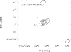
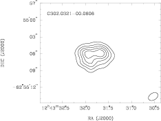
Figure 1: High resolution images of our UCHII and HCHII regions. The 18.496 and 19.520 GHz data have been combined to make a single 19.008 GHz image. The contours show 6 levels, equally spaced between $5\sigma$ and the image peak.

2.3.2 H$70\alpha$ radio recombination lines

Hydrogen recombination lines are a customary diagnostic for HII regions. In the 2006 September 18 snapshot observing run with the H75 hybrid array, we used the second frequency band to observe the H$70\alpha$ radio recombination line (rest frequency 18.769 GHz). The resulting velocity resolution was 250 kHz (4 km s^-1) with a total velocity coverage for each spectrum measurement of $\sim$500 km s^-1. For the H$70\alpha$ transition in a typical HII region, the observed spectral line is predicted to be approximately 5% of the peak flux of the associated continuum source, which was well within our sensitivity limits. The eight sources presented here all had a clear H$70\alpha$ detection, as shown in the spectra plotted in Fig. 2.

Figure 2: H$70\alpha$ radio recombination line spectra for our UCHII and HCHII regions showing the mean flux density in a $2\times 2$ pixel region centred on the source position.

2.3.3 High frequency observations

On 2008 July 10 we observed seven of the eight sources (excluding G301.1366-00.2248) at 33 GHz (central frequencies 32.064 GHz and 34.112 GHz) and 44 GHz (central frequencies 42.944 GHz and 44.992 GHz) as part of the ongoing ATCA calibrator program (C007). We also observed seven of the eight sources at 95 GHz (central frequencies 93.504 GHz and 95.552 GHz).

All observations were done in continuum mode with a 128 MHz bandwidth on each of the two central frequencies, sub-divided into 32 channels. We used the H214 hybrid array, with baselines from 92 m to 247 m. We observed one or two cuts for each object, with a typical total integration time of a few minutes. This is not enough to do meaningful imaging, but is sufficient to measure the angular size and flux density accurately. The smallest scale these observations are sensitive to is roughly 5–6″at 33 GHz and 44 GHz and 2″at 95 GHz.

The planet Uranus was used as the primary flux calibrator. Calibration at these high frequencies can be problematic, which is one of the motivations for searching for new UCHII candidates as potential flux calibrators for the ATCA.

The remaining object, G301.1366-00.2248, was observed on 2009 September 01 as part of the C2050 calibrator program. We obtained data at 33, 44 and 46 GHz using the EW352 array, with baselines from 31 m to 352 m.

2.3.4 Radio properties of the sample

The observational attributes of the sources are shown in Table 2. These include our measured flux densities in Janskys; the Gaussian-fitted angular sizes at 18.624 GHz, ($\theta$) in arcsec; the recombination line-to-continuum ratios ($F_{L}$/$F_{C}$); $V$, the LSR radial velocity of the recombination line in km s^-1; and, in the final column, the ratios of spatially integrated 8.0-$\mu$m fluxes to those at 843 MHz. This ratio provides a discriminant between thermal and non-thermal radio emission (Cohen & Green, 2001). MIR/radio continuum ratios have been measured for ensembles of thermal emission sources, in particular for HII regions of different morphologies (Cohen & Green, 2001) and planetary nebulae (Cohen et al., 2007). Non-thermal sources, for example galaxies and supernova remnants, are about 400 times weaker than a thermal source of equivalent radio intensity.

The errors in the flux densities are a function of the RMS noise, systematic errors in the calibration, and errors associated with our method of measurement. The listed flux densities at high frequencies are dominated by systematic calibration uncertainties, which are hard to estimate. In Table 2 we have given an overall estimate of the percentage error at each frequency.

Table 2: Measured attributes of the sources, including flux densities in Janskys, recombination line ratios ($F_{L}/F_{C}$) and velocities (V) in km s^-1, and MIR/radio flux ratios.

Name	$f_{0.843}$	$f_{18.624}$	$\theta$(”)	$F_{L}$/$F_{C}$	V	$f_{19.008}$	$f_{32.064}$	$f_{42.944}$	$f_{44.992}$	$f_{95}$	MIR/$f_{0.843}$
	($\pm 5\%$)	($\pm 10\%$)				($\pm 10\%$)	($\pm 10\%$)	($\pm 10\%$)	($\pm 10\%$)	($\pm 10\%$)
G301.1366$-$00.2248	0.012	1.03	0.7	0.053	$-20$	0.9	1.6	1.7	1.8	$-$	$200\pm 30$
G302.0321$-$00.0606	0.274	0.99	4.0	0.219	$-31$	1.0	1.0	1.0	0.9	1.2	$45\pm 2$
G307.5604$-$00.5875	0.446	0.74	8.0	0.224	$-41$	0.8	0.8	0.8	0.7	0.8	$40\pm 2$
G309.9217$+$00.4788	0.028	1.02	1.0	0.163	$-63$	1.1	1.1	1.2	1.1	3.1	$450\pm 50$
G323.4594$-$00.0788	0.094	0.98	2.0	0.106	$-75$	$-$	1.3	1.3	1.3	3.1	$90\pm 10$
G328.8076$+$00.6330	0.224	1.91	4.4	0.203	$-44$	$-$	2.1	2.1	2.0	4.2	$30\pm 3$
G330.9536$-$00.1820	0.151	3.77	1.8	0.102	$-91$	5.0	6.0	6.8	6.5	21.0	$16\pm 2$
G332.8254$-$00.5499	0.669	4.76	3.0	0.189	$-69$	7.1	6.0	6.0	5.8	14.5	$80\pm 10$

3 Analysis

Recombination lines can be characterised as Gaussian profiles with a peak $F_{L}$, a central velocity $V$ and a FWHM velocity $\Delta V$. The line velocity can be used to estimate a kinematic distance for the object, which then determines its linear size and subsequent classification. The line width is used to calculate the electron temperatures ($T_{e}$) and any broadening becomes a useful discriminant between HCHII and UCHII regions. The derived parameters calculated in this section are given in Table 3. Also included in Table 3 are extinction values calculated using the optical depth of silicate features in the IRAS Low Resolution Spectrometer (LRS) spectra, as discussed in Section 6.3.

Table 3: Summary of quantities derived from pure free-free, constant density model fits to observations from 843 MHz$-$45 GHz.

Name	$\alpha^{20}_{0.843}$	Te	$\Delta$V	Dist.	Size	EM	Ne	AV	95/45 GHz	Class
		(K)	(km s-1)	(kpc)	(pc)	(pc cm-6)		(mag)	flux ratio
G301.1366$-$00.2248	1.5	11600	66	4.5	0.02	3.0E+09	6.8E+05	$11\pm 1$	…	H
G302.0321$-$00.0606	0.4	8000	24	7.2	0.14	3.0E+07	1.5E+04	$20\pm 2$	1.6	U
G307.5604$-$00.5875	0.2	7100	27	7.7	0.30	5.0E+06	4.1E+03	$60\pm 5$	…	U
G309.9217$+$00.4788	1.2	6700	40	5.5	0.03	8.0E+08	2.3E+05	$40\pm 3$	2.0	H
G323.4594$-$00.0788	0.8	8100	50	4.8	0.05	1.9E+08	6.4E+04	$18\pm 1$	2.9	H
				8.9	0.09		4.7E+04			U–H
G328.8076$+$00.6330	0.7	6400	34	11.7	0.25	6.0E+07	1.6E+04	$50\pm 4$	2.5	U
G330.9536$-$00.1820	1.1	10400	38	5.5	0.05	1.3E+09	1.6E+05	$9\pm 1$	3.5	H
				9.3	0.08		1.2E+05			U–H
G332.8254$-$00.5499	0.7	6500	36	4.4	0.06	4.0E+08	8.0E+04	…	1.8	U

3.1 Electron and brightness temperatures

The continuum and recombination line brightness temperatures $T_{C}$ and $T_{L}$ can be calculated from the peak flux density using the Rayleigh-Jeans approximation

$$T_{B}=\frac{c^{2}}{2\nu^{2}k_{B}\Omega}S_{\nu}$$ (1)

where $\Omega$ is the solid beam angle.

We calculated the electron temperature $T_{e}$ for each object following (Condon, 2007) (Equation 7C5):

$$T_{e}\simeq\left[7\times 10^{3}\nu^{1.1}\frac{1}{1.08\Delta v}\frac{T_{c}}{T_{L}}\right]^{0.87}$$ (2)

which assumes LTE and that the typical He$+$/H$+$ ion ratio is N(He$+$)/N(H$+$)$\simeq 0.08$. These derived values are shown in Table 3 and are primarily of interest for the SED modelling in the next section. Note that since the recombination line width may be affected by other factors than just the temperature, our values of $T_{e}$ may be overestimated. However, this overestimate can not be large, or our SED’s will not fit the observed flux densities and sizes. For our data the uncertainties due to complexity of source shapes make $T_{e}$ estimates from the continuum alone unreliable but this does indicate that future higher quality and higher resolution imaging observations with flux densities and size measurements at a range of frequencies could be used to separate thermal broadening of the recombination lines from other effects.

3.2 Distance estimates

We calculated kinematic distances using the Galactic rotation curve of McClure-Griffiths & Dickey (2007)

$$\Theta(R)=\left(0.186\frac{R}{R_{0}}+0.887\right)\Theta_{0}$$ (3)

with $\Theta_{0}=220{\rm kms}^{-1}$ and the distance to the Galactic centre $R_{0}=8.5{\rm kpc}$. Four of our sources (G302.0321$-$00.0606, G307.5604$-$00.5875, G328.8076$+$00.6330, and G332.8254$-$00.5499) are included in the Caswell & Haynes (1987) study of southern HII regions, and our distances are in good agreement.

For those of our sources with a distance ambiguity, we followed Caswell & Haynes (1987) who resolved a number of such ambiguities by checking for optical counterparts. The argument is that sources with optical counterparts must be at the near distance because dust would obscure any object further than about 5 kpc. We took the same approach using the highly sensitive SuperCOSMOS H$\alpha$ Survey (Parker et al., 2005) and have attempted to refine the distance to which an object can be detected in H$\alpha$ as a function of Galactic longitude. We also consulted 2MASS K_s images to look for diffuse counterparts. The distance of 4.4 kpc for G332.8254$-$00.5499 was considered most likely based on a visual identification by Caswell & Haynes (1987).

Frew (priv. comm.) has determined reddenings for about 1000 ESO PNe listed by Acker et al. (1992) and Acker et al. (1996). These diminish around $E(B-V)$ of 3 (i.e. for extinction A${}_{V}\geq 9.3$). Frew notes that recently discovered PNe are impossible to detect in H$\alpha$ when A_Hα exceeds 7 mag., equivalent to A${}_{V}\sim$ 8.6 mag, consistent with his estimate from ESO PNe. Therefore, PNe can serve as a probe of the interstellar medium’s (ISM) average transparency. Mean values of extinction near the Galactic plane have been measured as a function of longitude by Joshi (2005) and vary from about 0.2 to 0.6 mag kpc^-1. The lowest reddening occurs for longitudes between 190°and 290°and the highest toward the Galactic Centre (Arenou et al., 1992; Chen et al., 1998; Joshi, 2005). For our HII regions, we expect to detect H$\alpha$ emission to a distance of 12, 6, and 5 kpc at longitudes of 270°, 300°and 330°, respectively. Non-detection of H$\alpha$ suggests that distances greater than these are more likely in a given direction. Using these guidelines we have resolved most of the distance ambiguities in Table 3, putting the most likely distance in the table. When we have been unable to decide (e.g. in the absence of any optical and even a near-infrared counterpart), two models for that source have been calculated, corresponding to both distances.

4 SED models

The spectral energy distributions (SED) for each of our eight objects are shown in Fig. 3. The flux densities increase from 843 MHz to 95 GHz (or the highest frequencies for sources not observed at all bands). Table 3 tabulates quantities derived from constant density models fit to the SEDs over the range 843 MHz to 45 GHz. For each of the eight sources we give the observed recombination line temperature and line width, followed by the emission measure (EM), the predicted linear size, mean electron density, A_V, and our classification of the type of HII region based on all these data (U: ultra-compact or H: hyper-compact).

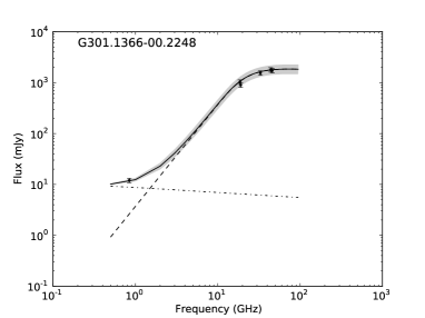
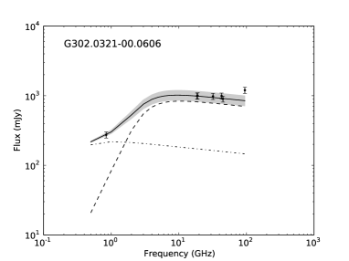
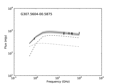
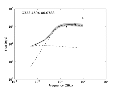
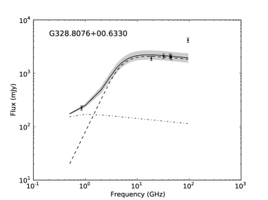
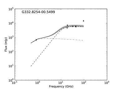
Figure 3: Spectral energy distributions and best fit models for our sample. The dashed line shows the fit to flux density points between 1 GHz and 45 GHz. The dotted line shows the additional component required to account for the 843 MHz flux density. The solid line represents the sum of the two components, with grey scale showing the range in fits allowed by a 10% change in measured source size.

We have modeled each source’s SED to find the best estimate for its physical parameters. The models also allow the flux density in the Planck Low Frequency Instrument (LFI) and High Frequency Instrument (HFI) bands to be estimated by interpolation or extrapolation. To model the SEDs we fit the component visibilities, measured source sizes and the recombination line electron temperature. We used the standard model for the electron density of an HII region, given by Mezger & Henderson (1967).

We estimated each source’s distance as described in Section 3.2. All flux densities were calculated by fitting the visibilities and extrapolating back to zero spacing. The errors associated with this process are shown on each point in Fig. 3. Any contribution from large scale diffuse emission was excluded. The source sizes were calculated by fitting a Gaussian to the 19 GHz visibilities. These sizes are accurate to $\pm 10\%$, and the range of allowed models is represented by grey shading in Fig. 3. If the output from the snapshot observations of cuts in hour angle were inconsistent with circular symmetry then the geometric mean size was used.

Given the angular size constraints from the visibility functions at all frequencies we have only one free parameter, the emission measure, which was calculated by. assuming free-free emission and fitting uniform density SEDs to the observed flux density distribution in the frequency range 1 GHz to 45 GHz. A second component (shown as a dotted line for each model in Fig. 3) was added to demonstrate that the higher than expected flux density measurement at 843 MHz can be explained by a diffuse component ($\sim 10\arcsec$ in size) surrounding the core of the UCHII region. Although this more diffuse component is not imaged directly, it is well constrained by the observations. It must be smaller than $\sim$45″or it would appear resolved in the MPGS-2 image and it must be larger than $10-20$″or it will violate the 20 GHz size and flux density. The corresponding emission measures are between $10^{4}$ and a few $\times 10^{5}$ pc cm^-6.

These simple models suffice to match the SEDs of G301.1366$-$00.2248 (which lacks data 95 GHz), G302.0321$-$00.0606 and G307.5604$-$00.5875. However, the rest of the objects all show sharp increases in flux between 45 GHz and 95 GHz. The most extreme case, G330.9536$-$00.1820, has a 95 GHz flux 3.5 times that measured at 45 GHz. This phenomenon is well established (e.g. Gibb & Hoare, 2007) though not well understood. Attempts to fit these by purely-free-free components fail to match the observed source sizes by requiring a smaller angular size at 95 GHz, whereas the visibilities indicate a diameter similar to that of the 19 GHz flux.

There is a tendency in the literature to characterize all HCHII region spectra as approximately $\nu^{+1}$ but there are significant variations even in our small sample. Nonetheless, the values are suggestive of the spectra found for (proto)planetary nebulae, and ionized stellar winds in general. Several groups have proposed explanations, interpreting the steep spectra as thermal emission either from constant density cores (Olnon, 1975), or a constant velocity wind with an r^-2 density distribution (Panagia & Felli, 1975; Wright & Barlow, 1975).

Further refinements were introduced by Marsh who proposed truncation of a constant velocity inverse-square stellar wind flow (Marsh, 1975), and acceleration of the stellar envelope by radiation pressure on dust grains in the wind (Marsh, 1976). All these approaches require the size of the unit optical depth surface to be frequency-dependent. Both mechanisms would steepen the spectral energy distribution of the radio emission, which constituted the essential constraint for modeling single dish data. This aspect of early models was successful. However, when one also has multi-wavelength data including visibilities from synthesis imaging at a range of antenna separations, the spatial scale of the radio-emitting envelope has further constraints and may not be consistent with an analysis of single dish observations.

Sewilo et al. (2004) allude to the possibility of clumping of the gas on an unresolved scale and this was discussed by Ignace & Churchwell (2004) and Gibb & Hoare (2007). If the 95 GHz (3 mm) free-free emission had a very small filling factor over the entire measured size then this component would become optically thick below 45 GHz (7 mm) and one could fit the rise at 95 GHz without violating the size constraint. It is possible that a thin shell or even the sharp edge of a shell, could provide the required small scale structure but more complete high resolution observations would be needed to confirm this.

Thermal emission by dust is more commonly invoked to account for the 95 GHz excess, particularly for sources where dust emission is shown to be a natural extension of the associated MIR and FIR spectral energy distribution (e.g. Sabbatini et al., 2005). This could be cold dust ($\sim$30 K) mixed into the molecular core (Brooks et al. in preparation) or warmer dust, heated by the embedded star(s) forming in the core, and expelled from the core into the envelope by a radiatively driven stellar wind.

Lizano (2008) argues that heating of grains by collisions with gas to their sublimation temperatures could not occur unless the gas densities exceeded $10^{9}{\rm cm}^{-3}$. We have also been able to model the high frequency excesses by a shell of hot dust ($\sim 800$ K) for which we require similar high mean densities $2\times 10^{9}{\rm cm}^{-3}$. Full radiative transfer modelling would be needed to verify this scenario. This should be guided by FIR observations, preferably with significantly higher resolution than IRAS to avoid confusion in the Galactic plane caused by unassociated point sources and widespread diffuse emission. MIPSGAL 70-$\mu$m images will be useful when they become available. The modelled dust contributions cannot be excluded solely from their implied temperatures. Our SEDs have the great merit of fitting all the data for a given source and hence we can estimate flux densities to satisfy the Planck LFI calibration requirements through interpolation.

The 843 MHz flux densities predicted from our simple models were lower (by up to a factor of 10) than our observed values. Assuming the excess flux densities are also produced by thermal emission then it is easy to match the observed values by adding an optically thin component of a larger size (typically $\sim 10\arcsec$) but with an emission measure of only 1% of the 19 GHz component. This dominates the 843 MHz emission yet does not perceptibly influence the high frequency fluxes. However, it is not possible to determine the size, temperature and EM of this component uniquely from our data because the resolution of the 843MHz data is too low to resolve this structure. We emphasize that this aspect of our models relates solely to the ionized volume surrounding the UCHII regions. These zones also support the idea (Kurtz et al., 1999) that every UCHII region is associated with an extensive low ionization halo sustained by leakage of UV photons from the compact core.

5 Criteria for ultra- and hyper-compact regions

To discriminate between ultra-compact (UC) and hyper-compact (HC) HII regions we have adopted standard quantitative criteria based on a survey of the literature (see, for example Kurtz, 2000, 2002, 2005; Wood & Churchwell, 1989; Afflerbach et al., 1996; Sewilo et al., 2004; Hoare, 2005). Typical ranges for these parameters (size, mean density, emission measure and recombination line width) are shown in Table 4.

Table 4: Quantitative criteria for UCHII and HCHII, summarised from the literature.

Parameter	UCHII	HCHII
Size	$<0.1$ pc	$<0.05$ pc
Mean density	$\geq$ 104 cm-3	$\geq$ 3$\times$ 105 cm-3
Emission measure	$\geq 10^{7}$pc cm-6	$\geq$ 108 pc cm-6
Recombination line width	$\leq 40{\rm kms}^{-1}$	$>40{\rm kms}^{-1}$

Fig. 4 shows the diameter of each HII region plotted against its emission measure (left) and recombination line width (right). The dashed lines represent the boundaries between UC and HC regions in each attribute, with UCHII expected to fall towards the top left quadrant, and HCHII towards the bottom right quadrant. The two sources (G323.4594$-$00.0788 and G330.9536$-$00.1820) for which we were unable to resolve the distance ambiguity are plotted twice (one for each distance) and connected with a line.

Figure 4: Left: HII region diameter vs. emission measure for the eight sources in our sample. Sources are identified with a truncated version of their full name. The two objects with unresolved distance ambiguities (G323.4594$-$00.0788 and G330.9536$-$00.1820) are plotted twice, corresponding to parameters derived for each distance, and their points are connected in the plot. Right: HII region diameter vs. the radio recombination line width. The dashed lines in each figure represent the demarcation between UCHII and HCHII candidates — the quadrant containing HCHII is indicated by arrows.

If the dust distribution surrounding these nascent high mass stars were always a disk then the orientation of that disk would govern the amount of extinction along the line of sight rather than the mean density or EM. G307.5604$-$00.5875 combines the highest measured extinction with the lowest EM, perhaps indicating that the dust envelopes are indeed flattened instead of spherical. No IRAS LRS spectrum is available for two of the three objects with the largest EMs. This might indicate that the extinction to these two regions is so large that the MIR emission from them simply cannot escape in our direction.

It is often argued that each HC region contains only a single star, where UC regions may have several associated stars. Of particular interest is the complexity clearly shown by the Spitzer MIR images in Fig. 7. In addition to the associated filaments and diffuse emission, the regions we have observed consist of small clusters of stars, probably at different stages of early evolution based on their IRAC false colours. Even if one tried rigorously to trace every such component star in an HII region from one wavelength region to the next it would be a gross oversimplification to define an infrared SED based on the sum of all flux within a given complex. The underlying issue is the variation of beam size with IR wavelength. Constructing a NIR-to-FIR SED from 2MASS, IRAC, MIPS, and IRAS would involve the mingling of data from instrumental beams whose FWHMs change across the resulting SED from 2.3, 1.9, 6, to about 25–100 arcsec, respectively. No individual entity in these regions is likely to match the shape of the total SED because the content of these beams would only very rarely consist of the same single entity at all wavelengths.

Inspection of the 95 GHz (3 mm) interferometer visibilities indicate that several of our HII regions have small structures present which are not present in the lower frequency visibilities (or images) where they are presumably optically thick. The visibilities of G323.4594$-$00.0788 clearly shows two components, with approximately half the flux ($\pm 20\%$) emitted by each component. Our 45 GHz data yields only the total flux and at 95 GHz we are dominated by the smaller component which we estimate as only 0$\aas@@fstack{\prime\prime}$7 in size. It is likely to be another hyper-compact source. In summary, our sample contains 2 hyper-compact sources (G301.1366$-$00.2248, G309.9217$+$00.4788), 4 ultra-compact sources (G302.0321$-$00.0606, G307.5604$-$00.5875, G328.8076$+$00.6330, G332.8254$-$00.5499), and two sources with attributes intermediate between hyper-compact and ultra-compact, with a final classification partly dependent on resolving their distance ambiguities (G323.4594$-$00.0788, G330.9536$-$00.1820).

6 Infrared Data

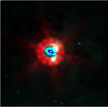
Figure 5: Spitzer IRAC-MIPS false colour $24\mu$m images of G301.1366$-$00.2248 and G309.9217$+$00.4788.

To further explore the nature of each radio-selected source we extracted images from four Spitzer Space Telescope Legacy projects. Firstly, GLIMPSE-I (Benjamin et al., 2003), which mapped the inner Galactic plane between longitudes $\pm 10$°and $\pm 65$°and latitudes $\pm 1$°using the InfraRed Array Camera (IRAC) (Fazio et al., 2004) at 3.6, 4.5, 5.8, and $8.0\mu$m. Secondly, the later GLIMPSE-II described by Churchwell et al. (2007) which completed the coverage of the Galactic Centre region and extended the latitude range to $\pm 2$°at the Centre. Finally, the MIPSGAL-I and MIPSGAL-II projects (Carey et al., 2005; Carey et al., 2007) which matched the GLIMPSE projects using the Multiband Imaging Photometer for Spitzer (MIPS) at 24, 70 and $160\mu$m.

The IRAC images provide spatial resolutions between 1$\aas@@fstack{\prime\prime}$5 and 1$\aas@@fstack{\prime\prime}$9 FWHM, comparable with that achieved by the ATCA at 20 GHz using the 6 km baseline. False-colour IRAC imagery is valuable in diagnosing the nature of the IR emission process in a wide variety of objects. Cohen et al. (2007) have discussed the values for coding IRAC images of HII regions so that blue, green and red represent 4.5, 5.8 and 8.0 $\mu$m, respectively. Structures that appear yellow in the resulting 3-colour images are indicative of sources in which polycyclic aromatic hydrocarbons (PAHs) dominate the emission. By contrast, regions that appear white trace broadband thermal emission by heated dust, indicative of the MIR-emitting surface of the cocoon. White regions represent less evolved structures than yellow regions.

The spatial resolution of MIPS at $24\mu$m is $\sim 6\arcsec$, substantially poorer than that of IRAC. However, its ability to trace thermal emission from cool circumstellar dust (temperature around 120 K) surrounding deeply embedded massive stars is an important tool for isolating the youngest object in a group of sources. We made 3-colour Spitzer images that combine IRAC 5.8, 8.0 and MIPS $24\mu$m images as blue, green and red, respectively to define the locations of cooler thermally emitting dust. The $24\mu$m images were from the 2007 October release of enhanced MIPSGAL images, described by Carey et al. (2009). The $24\mu$m peaks always coincide with the white IRAC sources and PAH emission would appear turquoise in the IRAC-MIPS combined colours as demonstrated in Fig. 5.

6.1 Comparison of high resolution MIR and radio observations

Our high resolution 19 GHz images have almost the same spatial resolution as the IRAC images and hence are invaluable for associating the dominant radio emission of a region with specific MIR components. Fig. 6 shows our 19 GHz continuum images (as contours), overlaid on grey-scale $8\mu$m images, which enables us to locate the origin of the radio emission. These indicate that the radio peaks match the white IRAC sources and the $24\mu$m peaks.

For example, the most well studied source in the set, G301.1366$-$00.2248 (see Henning et al., 2000) appears to consist of about 6 separate MIR components, some diffuse. Yet radio emission is found from only two of these objects, and the stronger radio component is far brighter than the second radio source in this complex. This is important because this region also has the highest recombination line width in our sample. This 66 km s^-1 line width is intrinsic. It could not arise simply by overlaying lines from the two radio components.

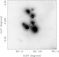
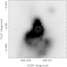
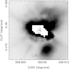
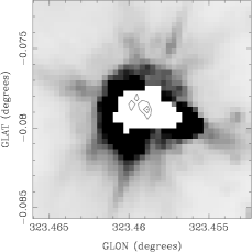
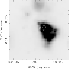
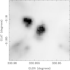
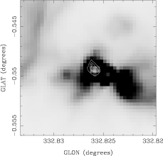
Figure 6: Overlays of MIR and high resolution 19 GHz images demonstrating the relationship between radio emission and the MIR structure of these regions. The white contours (or black contours in the cases where the MIR image is saturated) of radio emission show 3 levels, equally spaced between $5\sigma$ and the image peak. Sources shown from left to right then top to bottom are: G301.1366$-$00.2248; G302.0321$-$00.0606; G307.5604$-$00.5875; G309.9217$+$00.4788; G323.4594$-$00.0788; G328.8076$+$00.6330; G330.9536$-$00.1820; and G332.8254$-$00.5499.

6.2 MIR morphologies

High spatial resolution MIR views of our sample are provided by the false-colour IRAC images shown in Fig. 7. From these, one can appreciate that: (i) MIR and radio morphologies of these sources are totally different; (ii) our sample shows a diversity of MIR structures; (iii) most objects consist of clusters of MIR point sources or small extended sources, often in association with diffuse emission and/or separate bright MIR sources. Most of the point sources that constitute these small groups are yellow (indicative of PAH emission) but a small number (typically only one) of the cluster members are white, suggesting thermal radiation by warm dust grains which emit in all three of the IRAC bands. These white objects are always the brightest elements of the MIR groups. When such an ultra-compact MIR object is detected it is always closely accompanied either by other, fainter, sources or diffuse emission, or both. Turquoise cores arise because of saturation in the IRAC arrays. Red, orange or yellow diffuse emission is often observed around the small groups, again suggesting widespread PAH emission as Cohen et al. (2007) found for spatially extended HII regions.

The MIR counterparts of G309.9217$+$00.4788 and G323.4594$-$00.0788 contain obvious indications of an unresolved source as evidenced by the diffraction spikes from the Spitzer telescope as seen in the IRAC images. There is no relationship between MIR and radio morphologies for HII regions in general (Cohen et al., 2007) and there appears to be none for HCHII and UCHII regions either.

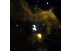
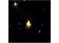
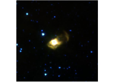
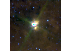
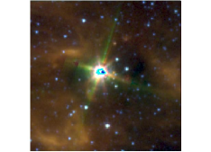
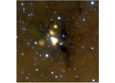
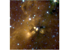
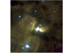
Figure 7: MIR false-colour images of UCHII regions. For the Spitzer images we used blue, green, red for images at 4.5, 5.8, 8.0 $\mu$m bands, respectively. Sources shown from left to right then top to bottom are: G301.1366$-$00.2248; G302.0321$-$00.0606; G307.5604$-$00.5875; G309.9217$+$00.4788; G323.4594$-$00.0788; G328.8076$+$00.6330; G330.9536$-$00.1820; and G332.8254$-$00.5499.

6.3 Extinction within UCHII regions

We have examined false-colour images based on 2MASS $JHK$ bands to aid interpretation of the MIR images. However, very few near-infrared (NIR) counterparts to the UCHII regions are found, presumably due to heavy obscuration. In order to test this presumption and to estimate the total line-of-sight extinction toward our sources we have sought spectra from the complete IRAS LRS database of 171 000 spectra from 7.7$-$22.7 $\mu$m. All spectra were recalibrated by Cohen et al. (1992). Fig. 8 shows a representative spectrum for the source G323.4594$-$00.0788. The most obvious features are deep amorphous silicate absorption bands near 10 and $18\mu$m. These arise as light from the embedded MIR-bright central star suffers heavy extinction along the line-of-sight within the dusty circumstellar cocoon.

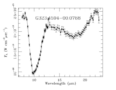
Figure 8: IRAS LRS spectrum of G323.4594$-$00.0788 showing the deep silicate absorptions.

The $10\mu$m optical depths of the silicate features can be converted into measures of the associated extinction by multiplying by $18.5\pm 1.5$ (Roche & Aitken, 1984). In several regions the silicate absorption at $10\mu$m is so severe that the LRS data fall to zero. In such spectra the $18\mu$m absorption band is still readily detected and we estimate a median of 5.3 for the ratio of $\tau_{10\,\mu m}/\tau_{18\,\mu m}$ for a much larger sample of HII regions than are represented here. In this way we have derived line-of-sight extinctions for 7 of the 8 sources in this paper. The expectation is that almost all of this extinction arises solely within the dusty shell that still envelops each of these regions, rather than in the intervening interstellar medium.

7 Conclusions

We present a sample of eight hyper- and ultra-compact HII regions, identified as part of a blind survey for ultra-compact HII regions. These are part of a larger set of 46 objects, identified on the basis of their 20 GHz to 843 MHz radio flux density ratio. These sources are some of the brightest compact sources in the Southern sky at 20 GHz. The basis for this work are two new surveys of the southern sky — the Australia Telescope 20 GHz survey and the second epoch Molonglo Galactic Plane Survey at 843 MHz.

We have classified each source as hyper- or ultra-compact on the basis of their emission measures, sizes, and radio recombination line width, resulting in 2 HCHII, 4 UCHII and 2 sources that are undetermined between these classifications because of an ambiguity in their kinematic distances. Using MIR and radio images at comparable resolution we have shown that, on the smallest scales that we can explore, the MIR morphologies of these sources are completely different from their radio morphologies. The MIR images show that UCHII regions are rarely simple, and what appears to be a single object at lower resolution may actually be a complex cluster of young stars. The high frequency radio emission is useful for picking out the youngest objects in these clusters.

We have modelled the spectral energy distributions with a uniform density model assuming free-free emission. A majority of the objects show excess emission at the highest frequency, with the flux density at 95 GHz up to three times the flux density at 45 GHz. The confirms similar observations of young stellar objects by Gibb & Hoare (2007). To explain this excess we require a more sophisticated model than the one used here. For example, clumpiness of the gas on unresolved scales could produce the observed flux densities without violating the size constraints. Another alternative is the presence of cold dust mixed into the molecular core, or warmer dust formed in the core and then expelled into the envelope by a stellar wind. To investigate these possibilities higher resolution imaging in radio and the FIR are required.

7.1 Suitable calibration sources

An important goal which we have attempted to address was to identify calibrators so that Plank’s LFI could monitor the Galactic plane foreground emission. Our observations span the range from 0.8 to 95 GHz, covering the entire range of wavelengths for LFI (30, 44, 70 GHz). To extend to the 100 GHz channel of the HFI requires only minimal extrapolation of our models of these HII regions. Our objects were chosen on the basis of being compact and isolated (based on MGPS-2 observations) and as such are candidates for Planck calibrators.

In addition, these sources may be useful as 45 GHz (7 mm) and 95 GHz (3 mm) primary flux calibrators or secondary calibrators) for the Australia Telescope Compact Array. A subset of these sources are now being monitored as part of the C007 and C2050 calibration programs. It should be noted that the sources with excess emission at 95 GHz can not be explained by current models, and hence high frequency flux densities can not be extrapolated from our SEDs.

References

- Acker et al. (1996) Acker A., Marcout J., Ochsenbein F., 1996, First Supplement to the Strasbourg - ESO catalogue of galactic planetary nebulae. Garching: European Southern Observatory
- Acker et al. (1992) Acker A., Marcout J., Ochsenbein F., Stenholm B., Tylenda R., 1992, Strasbourg - ESO catalogue of galactic planetary nebulae. Garching: European Southern Observatory
- Afflerbach et al. (1996) Afflerbach A., Churchwell E., Acord J. M., Hofner P., Kurtz S., Depree C. G., 1996, ApJS, 106, 423
- Arenou et al. (1992) Arenou F., Grenon M., Gomez A., 1992, A&A, 258, 104
- Benjamin et al. (2003) Benjamin R. A., Churchwell E., Babler B. L., et al., 2003, PASP, 115, 953
- Bock et al. (1999) Bock D. C.-J., Large M. I., Sadler E. M., 1999, AJ, 117, 1578
- Carey et al. (2007) Carey S. J. Mizuno D. R., Kraemer K. E., Shenoy S., Noriega-Crespo A., Price S. D., Paladini R., Kuchar T. A., 2007, MIPSGAL v1.0 Data Delivery Description Document, http://data.spitzer.caltech.edu
- Carey et al. (2009) Carey S. J., Noriega-Crespo A., Mizuno D. R., et al., 2009, PASP, 121, 76
- Carey et al. (2005) Carey S. J., Noriega-Crespo A., Price S. D., et al., 2005, in Bulletin of the American Astronomical Society Vol. 37, MIPSGAL: A Survey of the Inner Galactic Plane at 24 and 70 microns, Survey Strategy and Early Results. pp 1–16
- Caswell & Haynes (1987) Caswell J. L., Haynes R. F., 1987, A&A, 171, 261
- Chen et al. (1998) Chen B., Vergely J. L., Valette B., Carraro G., 1998, A&A, 336, 137
- Churchwell et al. (2007) Churchwell E., Watson D. F., Povich M. S., et al., 2007, The Bubbling Galactic Disk II: the Inner 20 Degrees, http://www.astro.wisc.edu/glimpse/BubblesII_V2.pdf
- Cohen & Green (2001) Cohen M., Green A. J., 2001, MNRAS, 325, 531
- Cohen et al. (2007) Cohen M., Green A. J., Meade M. R., et al., 2007, MNRAS, 374, 979
- Cohen et al. (2007) Cohen M., Parker Q. A., Green A. J., et al., 2007, ApJ, 669, 343
- Cohen et al. (1992) Cohen M., Walker R. G., Witteborn F. C., 1992, AJ, 104, 2030
- Comeron & Torra (1996) Comeron F., Torra J., 1996, A&A, 314, 776
-
Condon (2007)
Condon J. J., 2007, Technical report, Essential Radio Astornomy,
http://www.cv.nrao.edu/course/astr534. National Radio Astronomy Observatory - Fazio et al. (2004) Fazio G. G., Hora J. L., Allen L. E., et al., 2004, ApJS, 154, 10
- Gaume et al. (1995) Gaume R. A., Goss W. M., Dickel H. R., Wilson T. L., Johnston K. J., 1995, ApJ, 438, 776
- Gibb & Hoare (2007) Gibb A. G., Hoare M. G., 2007, MNRAS, 380, 246
- Henning et al. (2000) Henning T., Lapinov A., Schreyer K., Stecklum B., Zinchenko I., 2000, A&A, 364, 613
- Hoare (2005) Hoare M. G., 2005, Astrophys. Space. Sci., 295, 203
- Hofner & Churchwell (1996) Hofner P., Churchwell E., 1996, A&AS, 120, 283
- Ignace & Churchwell (2004) Ignace R., Churchwell E., 2004, ApJ, 610, 351
- Joshi (2005) Joshi Y. C., 2005, MNRAS, 362, 1259
- Keto (2003) Keto E., 2003, ApJ, 599, 1196
- Kurtz (2002) Kurtz S., 2002, in Crowther P., ed., Hot Star Workshop III: The Earliest Phases of Massive Star Birth Vol. 267 of Astronomical Society of the Pacific Conference Series, Ultracompact HII Regions. p. 81
- Kurtz (2005) Kurtz S., 2005, in Cesaroni R., Felli M., Churchwell E., Walmsley M., eds, Massive Star Birth: A Crossroads of Astrophysics Vol. 227 of IAU Symposium, Hypercompact HII regions. pp 111–119
- Kurtz (2000) Kurtz S. E., 2000, in Arthur S. J., Brickhouse N. S., Franco J., eds, Revista Mexicana de Astronomia y Astrofisica Conference Series Vol. 9 of Revista Mexicana de Astronomia y Astrofisica Conference Series, Ultracompact H II Regions: New Challenges. pp 169–176
- Kurtz et al. (1999) Kurtz S. E., Watson A. M., Hofner P., Otte B., 1999, ApJ, 514, 232
- Lizano (2008) Lizano S., 2008, in Beuther H., Linz H., Henning T., eds, Massive Star Formation: Observations Confront Theory Vol. 387 of Astronomical Society of the Pacific Conference Series, Hypercompact HII Regions. p. 232
- Marsh (1975) Marsh K. A., 1975, ApJ, 201, 190
- Marsh (1976) Marsh K. A., 1976, ApJ, 203, 552
- Massardi et al. (2008) Massardi M., Ekers R. D., Murphy T., et al., 2008, MNRAS, 384, 775
- Mauch et al. (2003) Mauch T., Murphy T., Buttery H. J., Curran J., Hunstead R. W., Piestrzynski B., Robertson J. G., Sadler E. M., 2003, MNRAS, 342, 1117
- McClure-Griffiths & Dickey (2007) McClure-Griffiths N. M., Dickey J. M., 2007, ApJ, 671, 427
- Mezger & Henderson (1967) Mezger P. G., Henderson A. P., 1967, ApJ, 147, 471
- Mills (1981) Mills B. Y., 1981, Proceedings of the Astronomical Society of Australia, 4, 156
- Murphy et al. (2007) Murphy T., Mauch T., Green A., Hunstead R. W., Piestrzynska B., Kels A. P., Sztajer P., 2007, MNRAS, 382, 382
- Murphy et al. (2010) Murphy T., Sadler E. M., Ekers R. D., et al., 2010, MNRAS, in press, (astro-ph/0911.0002)
- Olnon (1975) Olnon F. M., 1975, A&A, 39, 217
- Panagia & Felli (1975) Panagia N., Felli M., 1975, A&A, 39, 1
- Parker et al. (2005) Parker Q. A., Phillipps S., Pierce M. J., et al., 2005, MNRAS, 362, 689
- Price et al. (2001) Price S. D., Egan M. P., Carey S. J., Mizuno D. R., Kuchar T. A., 2001, AJ, 121, 2819
- Robertson (1991) Robertson J. G., 1991, Australian Journal of Physics, 44, 729
- Roche & Aitken (1984) Roche P. F., Aitken D. K., 1984, MNRAS, 208, 481
- Sabbatini et al. (2005) Sabbatini L., Cavaliere F., dall’Oglio G., et al., 2005, A&A, 439, 595
- Sewilo et al. (2004) Sewilo M., Churchwell E., Kurtz S., Goss W. M., Hofner P., 2004, ApJ, 605, 285
- Wood & Churchwell (1989) Wood D. O. S., Churchwell E., 1989, ApJS, 69, 831
- Wright & Barlow (1975) Wright A. E., Barlow M. J., 1975, MNRAS, 170, 41