Searching for the earliest galaxies in the 21 cm forest

Abstract

We use a model developed by Xu et al. (2010) to compute the 21 cm line absorption signatures imprinted by star-forming dwarf galaxies (DGs) and starless minihalos (MHs). The method, based on a statistical comparison of the equivalent width ($W_{\nu}$) distribution and flux correlation function, allows us to derive a simple selection criteria for candidate DGs at very high ($z\geq 8$) redshift. We find that $\approx 18\%$ of the total number of DGs along a line of sight to a target radio source (GRB or quasar) can be identified by the condition $W_{\nu}<0$; these objects correspond to the high-mass tail of the DG distribution at high redshift, and are embedded in large HII regions. The criterion $W_{\nu}>0.37\,{\rm kHz}$ instead selects $\approx 11\%$ of MHs. Selected candidate DGs could later be re-observed in the near-IR by the JWST with high efficiency, thus providing a direct probe of the most likely reionization sources.

1 INTRODUCTION

The properties of the earliest galaxies, such as their star formation histories, masses, production of ionizing photons and their escape fraction, are crucial in understanding the reionization process, during which the previously neutral intergalactic medium (IGM) becomes totally ionized. Thanks to the availability of large ground-based and space telescopes, and improvements in the searching technique for Lyman Break Galaxies and Lyman-$\alpha$ Emitters, we are now tracing galaxy formation at progressively higher redshifts beyond 6 (see Bunker et al. 2009 for a review). Candidates at redshifts as high as $z\sim 10$ are newly reported from the analysis of the Hubble Ultra Deep Field (HUDF) (Bouwens et al., 2009). However, it is now believed that the galaxies that produced most of the necessary (re)ionizing photons were dwarfs (Choudhury & Ferrara, 2007) which are currently beyond our capability of direct detection. The forthcoming James Webb Space Telescope (JWST) will have the capabilities to directly detect the reionization sources at the faint end of the luminosity function. Still, given their faintness, long integration times will be required; hence, defining target candidate reionizing sources will be of primary importance to study them in spectroscopic detail.

Instead of looking at a specific galaxy directly, the redshifted 21 cm transition of HI traces the neutral gas either in the diffuse IGM or in non-linear structures, comprising the most promising probe of the reionization process (see e.g. Furlanetto, Oh & Briggs 2006 for a review). While the 21 cm tomography maps out the three dimensional structure of the 21 cm emission or absorption by the IGM against the cosmic microwave background (CMB) (e.g. Madau et al. 1997; Tozzi et al. 2000), the 21 cm forest observation detects absorption lines of intervening structures towards high redshift radio sources showing high sensitivity to gas temperature (Xu et al., 2009). The problem of the 21 cm forest signatures produced by different kinds of structures has been addressed by several authors. Carilli et al. (2002) presented a detailed study of 21 cm absorption by the mean neutral IGM as well as filamentary structures based on the simulations of Gnedin (2000), but their box was too small to account for large scale structures and was not able to resolve collapsed objects. Instead, Furlanetto & Loeb (2002) used a simple analytic model to compute the absorption profiles and abundances of minihalos and galactic disks. Later on, Furlanetto (2006) re-examined four kinds of 21 cm forest absorption signatures in a broader context, especially the transmission gaps produced by ionized bubbles.

Recently, Xu et al. (2010) developed a more detailed model of the 21 cm absorption lines of minihalos (i.e. starless galaxies, MHs) and dwarf galaxies (star-forming galaxies, DGs) during the epoch of reionization, explored the physical origins of the line profiles, and generated synthetic spectra of the 21 cm forest on top of both high-$z$ quasars and gamma ray burst (GRB) afterglows. Interestingly, they find that: (i) MHs and DGs show very distinct 21 cm line absorption profiles (ii) they contribute differently to the spectrum due to the mass segregation between the two populations. It follows that it is in principle possible to build a criterion based on the 21 cm forest spectrum to efficiently select DGs.

The goal of this work is to derive the different signatures of DGs and MHs using a 21 cm spectrum of high-$z$ radio sources, and provide a criterion to pick DGs lines in the spectrum. For these candidates, precise redshift information will be available; moreover, given the angular position of the background source, the 21 cm forest observation provides an excellent tool for locating the high-$z$ DGs. The great advantage of using high-$z$ GRBs as background radio sources is that the follow-up IR JWST observations after the afterglow has faded away will not be hampered by the presence of a very luminous source (as in the case of a background quasar) in the field.

2 METHOD

Here we briefly summarize the main features of the model used in this work, but refer the interested reader to Xu et al. (2010) for a more comprehensive description. We use the Sheth-Tormen halo mass function (Sheth & Tormen, 1999) to model the halo number density at high redshift in the mass range $10^{5-10}M_{\odot}$, which covers the minimum mass allowed to collapse (Abel et al., 2000; O^′Shea & Norman, 2007) and most of the galaxies that are responsible for reionization (Choudhury & Ferrara, 2007). The dark matter halos have an NFW density profile within the virial radii $r_{\rm vir}$ (Navarro, Frenk & White, 1997), with a concentration parameter fitted to high-redshift simulation results by Gao et al. (2005); the dark matter density and velocity structure outside $r_{\rm vir}$ are described by an “Infall model” (Barkana, 2004). The gas inside the $r_{\rm vir}$ is assumed to be in hydrostatic equilibrium at temperature $T_{\rm vir}$ in the dark matter potential, while the gas outside follows the dark matter overdensity and velocity field.

Once the halo population is fixed, a timescale criterion for star formation is introduced to determine whether a halo is capable of hosting star formation. The timescale required for turning on star formation is modeled as the maximum between the free-fall time $t_{\rm ff}$ and the H₂ cooling time $t_{\rm cool}$ (Tegmark et al., 1997), i.e. $t_{\rm SB}=\max\{\,t_{\rm ff},\,t_{\rm cool}\,\}$. Then star formation activity begins at $t_{\rm s}=t_{\rm F}+t_{\rm SB}$, where $t_{\rm F}$ is the halo formation time predicted by the standard EPS model (Lacey & Cole, 1993). If $t_{\rm s}$ is larger than the Hubble time at the halo redshift, we define the system as a minihalo, i.e. a starless galaxy. The ionized fraction in a MH is computed with collisional ionization equilibrium, which depends on its temperature. The gas within $r_{\rm vir}$ is at the virial temperature, and in the absence of an X-ray background the gas outside is adiabatically compressed, so that the temperature is simply $T_{\rm K}=T_{\rm IGM}(1+\delta)^{\gamma-1}$, where $\gamma=5/3$ is the adiabatic index for atomic hydrogen, and $T_{\rm IGM}$ is the temperature of the mean-density IGM. The Ly$\alpha$ photons inside a MH are produced by recombinations, which are negligible for most MHs that are almost neutral, but serve as a dominant coupling source for the most massive MHs which are partially ionized due to their higher $T_{vir}$.

When the criterion $t_{\rm s}<t_{\rm H}$ is satisfied, star formation occurs within a Hubble time turning the halo into a dwarf galaxy. We use a mass-dependent handy fit of star formation efficiency provided by Salvadori & Ferrara (2009). Adopting the spectra of high redshift starburst galaxies provided by Schaerer (2002, 2003) and an escape fraction of $f_{\rm esc}=0.07$ as favored by the early reionization model (ERM, Gallerani et al. 2008), we numerically follow the expansion of the HII region. The gas temperature inside the HII region is fixed at $2\times 10^{4}{\rm K}$, while the temperature of gas around the HII region is calculated including the Hubble expansion, soft X-ray heating and the Compton heating. Although the soft X-ray heating dominates over the Compton heating, its effect is weak unless the DG has a higher stellar mass and/or a top-heavy initial mass function. Besides ionization and heating effects, the DG metal-free stellar population produces Ly$\alpha$ photons from soft X-ray cascading, which could penetrate into the nearby IGM and help to couple the spin temperature to the kinetic temperature of the gas. Finally, we account for the Ly$\alpha$ background produced by the collective contribution of DGs.

With the detailed modeling of properties of both MHs and dwarf galaxies, and an associated Ly$\alpha$ background, we compute the 21 cm absorption lines of these non-linear structures. The diffuse IGM creates a global decrement in the spectra of high-$z$ radio sources, on top of which MHs and DGs produce deep and narrow absorption lines. The 21 cm optical depth of an isolated object is (Field, 1959; Madau et al., 1997; Furlanetto & Loeb, 2002):

$$\tau(\nu) = \frac{3\,h_{\rm P}\,c^{3}A_{10}}{32\,\pi^{3/2}k_{\rm B}}\,\frac{1}{\nu^{2}}$$ (1)

$$\times \int_{-\infty}^{+\infty}\frac{n_{\rm HI}(r)}{b(r)T_{\rm S}(r)}\,\exp\left[\,-\,\frac{(u(\nu)-\bar{v}(r))^{2}}{b^{2}(r)}\,\right]dx,$$

where $A_{10}=2.85\times 10^{-15}\,{\rm s}^{-1}$ is the Einstein coefficient for the spontaneous decay of the 21 cm transition, $n_{\rm HI}$ is the neutral hydrogen number density, $T_{\rm S}$ is the spin temperature, and $b(r)$ is the Doppler parameter of the gas, $b(r)=\sqrt{\,2\,k_{\rm B}T_{K}(r)/m_{\rm H}}$. Here $u(\nu)$ is the frequency difference from the line center in terms of velocity, $u(\nu)\equiv c\,(\nu-\nu_{10})/\nu_{10}$, where $\nu_{10}=1420.4\,{\rm MHz}$ is the rest frame frequency of the 21 cm line, and $\bar{v}(r)$ is bulk velocity of gas projected onto the line of sight at radius $r$. Inside of the virial radius, the gas is thermalized, and $\bar{v}(r)=0$, while the gas outside the virial radius has a bulk velocity contributed from both infall and Hubble flow, which is predicted by the “Infall Model.” The coordinate $x$ is related to the radius $r$ by $r^{2}=(\alpha\,r_{\rm vir})^{2}+x^{2}$, where $\alpha$ is the impact parameter of the penetrating line of sight in units of $r_{\rm vir}$.

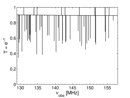
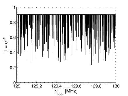
Figure 1: Relative transmission along a line of sight. Left: the spectrum with absorptions caused by DGs alone from 129$\,{\rm MHz}$ to 158$\,{\rm MHz}$ corresponding to $z=10.01$ – $7.99$. Right: the spectrum with absorptions caused by MHs alone from 129$\,{\rm MHz}$ to 130$\,{\rm MHz}$ corresponding to $z=10.01$ – $9.93$.

The spin temperature of neutral hydrogen is defined by the relative occupation numbers of the two hyperfine structure levels, and it is determined by (Field, 1958; Furlanetto, Oh & Briggs, 2006):

$$T_{\rm S}^{-1}\,=\,\frac{T_{\gamma}^{-1}+x_{c}\,T_{\rm K}^{-1}+x_{\alpha}\,T_{\rm C}^{-1}}{1+x_{c}+x_{\alpha}},$$ (2)

where $T_{\gamma}=2.726(1+z)\,{\rm K}$ is the CMB temperature at redshift $z$, $T_{\rm K}$ is the gas kinetic temperature, and $T_{\rm C}$ is the effective color temperature of the UV radiation. In most cases, $T_{\rm C}=T_{\rm K}$ due to the frequent Ly$\alpha$ scattering (Furlanetto, Oh & Briggs, 2006). The collisional coupling is described by the coefficient $x_{c}$, and $x_{\alpha}$ is the coupling coefficient of the Ly$\alpha$ pumping effect known as the Wouthuysen-Field coupling (Wouthuysen, 1952; Field, 1958). The main contributions to $x_{c}$ are H-H collisions and H-$e^{-}$ collisions, which can be written as $x_{c}\,=\,x_{c}^{\rm eH}+x_{c}^{\rm H\!H}\,=\,(n_{e}\,\kappa_{10}^{\rm eH}/A_{10})\,(T_{\star}/T_{\gamma})+(n_{\rm HI}\,\kappa_{10}^{\rm H\!H}/A_{10})\,(T_{\star}/T_{\gamma})$, where $T_{\star}=0.0682\,{\rm K}$ is the equivalent temperature of the energy splitting of the 21 cm transition, and $\kappa_{10}^{\rm eH}$ and $\kappa_{10}^{\rm H\!H}$ are the de-excitation rate coefficients in collisions with free electrons and hydrogen atoms, respectively. The coupling coefficient $x_{\alpha}$ is proportional to the total scattering rate between Ly$\alpha$ photons and hydrogen atoms, $x_{\alpha}\,=\,(4\,P_{\alpha}/27\,A_{10})\,(T_{\star}/T_{\gamma})$, where the scattering rate $P_{\alpha}$ is given by $P_{\alpha}\,=\,c\,\sigma_{\alpha}\,n_{\alpha}^{\rm tot}/\Delta\nu_{D}\,=\,4\pi\,\sigma_{\alpha}J_{\alpha}$. Here $\sigma_{\alpha}\equiv{\displaystyle\frac{\pi e^{2}}{m_{e}c}f_{\alpha}}$ where $f_{\alpha}=0.4162$ is the oscillator strength of the Ly$\alpha$ transition, $n_{\alpha}^{\rm tot}$ is the total number density of Ly$\alpha$ photons, $J_{\alpha}$ is the number intensity of the Ly$\alpha$ photons, and $\Delta\nu_{D}=(b/c)\,\nu_{\alpha}$ is the Doppler width with $b$ being the Doppler parameter and $\nu_{\alpha}$ being the Ly$\alpha$ frequency.

3 RESULTS

3.1 The spectra of dwarfs and minihalos

With the halo number density predicted by the Sheth-Tormen mass function and the cross-sectional area of halos determined by the mean halo separation, we derive the number density of the absorption lines. Applying our star formation criterion to each intersected halo with Monte-Carlo sampled mass and formation-redshift, we compute the absorption lines of MHs in collisional ionization equilibrium or DGs photoionized by central stars, and generate a synthetic spectrum along a line of sight. The entire spectrum with absorptions of both MHs and DGs is shown in Xu et al. (2010) against a quasar or a GRB afterglow. In order to illustrate the differences between the spectrum caused by MHs and that by DGs, and disregarding the background source properties, we plot the relative transmission $T=\exp(-\,\tau)$ of a spectrum with absorptions caused by dwarf galaxies alone (DG-spectrum) in the left panel of Fig.1 and that with absorptions caused by MHs alone (MH-spectrum) in the right panel, respectively. Note that the ranges of observed frequency are different in the two panels. The absorption lines are very narrow and closely spaced in the MH-spectrum which resembles a 21 cm forest, while the 21 cm lines on the DG-spectrum are much rarer. A clear signature unique to the DG-spectrum is that there are some dwarf galaxies with sufficiently large HII regions that give rise to leaks (i.e. negative absorption lines with equivalent width $W_{\nu}<0$) on the spectrum rather than absorption lines. Also, we see that absorption lines of MHs are generally deeper than DGs.

We define $\delta(\nu)$ to be the relative difference between the flux $f$ at observed frequency $\nu$ and the global flux transmitted through the homogeneous IGM at the corresponding redshift,

$$\delta(\nu)\,\equiv\,\frac{f(\nu)}{f_{\rm IGM}}-1.$$ (3)

Then we compute the flux correlation functions with the formula

$$\xi_{ab}(\Delta\nu)\,=\,\frac{1}{N}\sum_{i=1}^{N}\,\delta_{a}(\nu_{i})\,\delta_{b}(\nu_{i}+\Delta\nu),$$ (4)

where $N$ is the total number of point pairs on the spectrum with a frequency distance of $\Delta\nu$. The subscript “ab” takes the values “gg” (“hh”) for the auto-correlation function of the DG (MH) spectrum, or “hg” for the cross-correlation between the MH and DG spectra.

We plot these correlation functions with solid curves in Fig.2. From the auto-correlation function of the DG-spectrum, we see little correlation on frequency separations larger than $10\,{\rm kHz}$, while little correlation on frequency separations larger than $1\,{\rm kHz}$ is seen in the MH-spectrum. This is what we could expect for a randomly generated spectrum with only the halo mass function. The correlation seen on smaller frequency separations just comes from the point pairs located within the same lines. The DGs have a longer correlation length because of their broader absorption lines or leaks, but the amplitude of the correlation is very low because they are rare.

In order to illustrate the contribution of those dwarfs with negative absorption, we calculated the auto-correlation function of the DG-spectrum with leaks excluded; the result is shown as the dashed curve in the upper panel of Fig.2. The correlation amplitude is smaller due to the reduced number of signals, and the correlation length is reduced by more than one order of magnitude. This shows that the broad signals are caused primarily by those leaks. In addition, comparing this dashed curve with the solid curve in the bottom panel, we find that on average, an absorption line of a DG is even narrower than that of a MH. This is because some of these DGs produce HII regions larger than $r_{\rm vir}$, and the absorption lines from the gas outside the virial radii but inside the HII region, which has the largest infalling velocities, are erased.

The cross-correlation function between the MHs and DGs can also be obtained in the same way. In this work we have not considered the clustering property of the MHs and DGs arising from large scale structure, so the flux cross-correlation should be zero, except for the Poisson fluctuations. Our computation confirms this expectation.

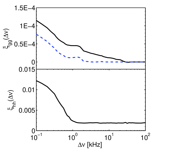
Figure 2: The flux correlation functions of the 21 cm forest spectrum. Upper panel: the auto-correlation functions of the DG-spectrum. The solid curve includes all the lines while the dashed curve excludes the leaks with $W_{\nu}<0$. Bottom panel: the auto-correlation function of the MH-spectrum. The spectra used for the computation here are all from 129$\,{\rm MHz}$ to 158$\,{\rm MHz}$ corresponding to $z=10.01$ – $7.99$.

3.2 Equivalent width distributions

Directly from the spectrum, we could compute the distribution of equivalent width (EW) of the absorption lines for a specific range of observed frequency corresponding to a specific redshift. As the continuum of a background source has a global decrement due to the absorption of the diffuse IGM, the real signal of non-linear structures is the extra absorption with respect to the flux transmitted through the IGM. Therefore, the EW of an absorption line should be defined as

$$W_{\nu} = \int\,\frac{\displaystyle f_{c}\,e^{-\,\tau_{\rm IGM}(z)}\,-\,f_{c}\,e^{-\,\tau(\nu)}}{\displaystyle f_{c}\,e^{-\,\tau_{\rm IGM}(z)}}\;d\nu$$ (5)

$$= \int\,{\displaystyle(1\,-\,e^{\tau_{\rm IGM}(z)\,-\,\tau(\nu)})}\;d\nu,$$

where $f_{c}$ is the continuum flux of the background radio source, and $\tau_{\rm IGM}(z)$ is the optical depth of the diffuse IGM at redshift $z$. We compute the differential and cumulative distributions of EW for the DG-spectrum in the left panel and for the MH-spectrum in the right panel respectively in Fig.3. The histograms represent the number distributions and the solid curves are the cumulative distributions per redshift interval.

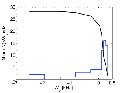
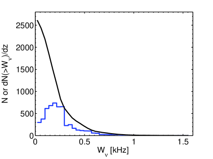
Figure 3: The differential and cumulative distributions of equivalent width of the 21 cm absorption lines. Left: the distribution for the DG-spectrum. Right: the distribution for the MH-spectrum. The spectra used for the computation here are both from 129$\,{\rm MHz}$ to 158$\,{\rm MHz}$ corresponding to $z=10.01$ – $7.99$.

We see that both EW distributions for DGs and MHs peak in the same region at $W_{\nu}\sim 0.1$ - $0.3\,{\rm kHz}$. This means that most of the dwarfs and MHs have comparable EWs, and we cannot distinguish them only from their EWs. However, the distribution curves of their EWs show different shapes. The EW distribution of DGs has a long tail at the small EW end, while MHs have a large-EW tail in the distribution curve.

3.3 Selection criteria

In this subsection, we aim at deriving a criterion to distinguish between the absorption lines caused by DGs and those caused by MHs.

From the computation of EW distributions, we find that only dwarf galaxies cause negative absorptions and thus have $W_{\nu}<0$, while only MHs are found to have EWs above $0.37\,{\rm kHz}$. Therefore, the first criterion for candidate DGs could be $W_{\nu}<0$, with which we select 10 dwarfs out of 54 in our synthetic spectrum. They have a 100 percent probability of being caused by DGs. That means, we can find $18.5\%$ of the total dwarfs along the line of sight, and they are relatively large dwarfs with large HII regions. In addition, with the predicted EW distribution, we can estimate the total number of DGs in the spectrum with the number of selected dwarf galaxies that have negative absorptions. Similarly, using the second criterion $W_{\nu}>0.37\,{\rm kHz}$, we can select 812 MHs out of a total of 7108. This is $11.4\%$ of all the MHs, which cannot be misidentified as DGs.

From the correlation functions shown above, on the other hand, we see that DGs have a longer correlation length than MHs. In the absence of halo clustering information, the correlation length reflects the mean width of the absorption lines, so this is also a distinctive signature of dwarfs from MHs. However, we have demonstrated that the correlation of dwarfs at relatively large frequency distances are exactly caused by those with negative absorptions. Therefore, the criterion of broad absorption is degenerate with the negative tail of the EW distribution of the DGs. Excluding those dwarfs with negative absorptions, the mean width of an absorption line of a DG (about $0.3\,{\rm kHz}$) is even smaller than that of an MH (about $0.5\,{\rm kHz}$). Hence, for the lines with $0<W_{\nu}<0.37\,{\rm kHz}$, if we have infinite resolution, a narrower absorption line will have a higher probability of being caused by a dwarf galaxy. This is probably beyond the resolution capabilities of currently planned instruments. The probability of these absorption lines being a DG would be $\sim 44/6296\sim 0.7\%$, with the complementary probability attributed to MHs.

4 DISCUSSION

Using the model developed by Xu et al. (2010), we have computed 21 cm absorption line spectra (“forest”) caused by DGs and MHs separately, their flux correlation functions and EW distributions, with the aim of distinguishing DGs from MHs in a statistical way. With the selection criterion of $W_{\nu}<0$, we are able to identify $\sim 18.5\%$ of DGs, and the criterion of $W_{\nu}>0.37\,{\rm kHz}$ selects $\sim 11.4\%$ of MHs. As a whole, we can disentangle $\sim 11.5\%$ of all the non-linear objects along a line of sight for which we can tell whether they are DGs or MHs. In this way, we find a strong but simple criterion to select candidate DGs to be later re-observed in the optical or infrared. Using the radio afterglow of a high redshift GRB as the background, this selection strategy could be accomplished by LOFAR or SKA. Then, after the GRB fades away, the follow-up observations can be carried out by JWST, which will be capable of directly detecting the DGs that are responsible for reionization.

Cosmic voids can also produce negative absorptions with respect to the mean absorption by the IGM. Accounting for the density voids requires the clustering information of large scale structure which is not included in our computation. However, according to the void size distribution based on the excursion set model developed by Sheth & Weygaert (2004), the characteristic scale of a density void is much larger than that of a DG HII region. As a result, density voids will produce “transmissivity windows” which are about one order of magnitude broader than the “leaks” produced by HII regions. As the width of both “transmissivity windows” and “leaks” exceed the current spectral resolution, a second criterion of signal width could be applied to eliminate those voids. Further, it is not necessary to consider the so-called “mixing problem” between the density voids and the HII regions as Shang et al. (2007) did for the Ly$\alpha$ forest, because the dwarfs are more likely to exist in filaments out of the voids, and they are not likely to mix with the density voids.

While the selection criterion for candidate DGs is reliable, the total number of predicted DGs and the percentages of identifiable objects are model-dependent. Specifically, they depend on the star formation law and efficiency, stellar initial mass function, and $f_{\rm esc}$. However, the fraction of dwarfs having negative absorption depends only on the shape of the EW distribution. If different star formation models predict similar shapes of the EW distribution, then our prediction of the fraction of dwarfs producing leaks is quite reliable and model-independent, and the total number of DGs along a given line of sight can be safely inferred from the number of selected leaks. Otherwise, we could compare the total number of dwarfs inferred from the percentage argument with the one originally predicted from our star formation model, and use this result to constrain the model.

To improve on the current selection criteria, the next step is to include the clustering properties of dark matter halos. With this ingredient included, the correlation functions will retain additional information on the distances between the lines. In principle, knowing the shape of the correlation function, one could associate to any given line in the spectrum (e.g. by using Bayesian methods) the statistical probability that it arises from a DG. We reserve these and other aspects to future work.

5 ACKNOWLEDGMENTS

We thank R. Barkana who provided his infall code. This work was supported in part by a scholarship from the China Scholarship council, by a research training fellowship from SISSA astrophysics sector, by the NSFC grants 10373001, 10533010, 10525314, and 10773001, by the CAS grant KJCX3-SYW-N2, and by the 973 program No. 2007CB8125401.

References

- Abel et al. (2000) Abel T., Bryan G. L., Norman M. L., 2000, ApJ, 540, 39
- Barkana (2004) Barkana R., 2004, MNRAS, 347, 59
- Bouwens et al. (2009) Bouwens R. J., Illingworth G. D., Labbé I., Oesch P. A., Carollo C. M., Trenti M., van Dokkum P. G., Franx M., Stiavelli M., González V., Magee D., submitted to Nature, arXiv:0912.4263
- Bunker et al. (2009) Bunker A., Stanway E., Ellis R., Lacy M, McMahon R., Eyles L., Stark D., Chiu K., 2009, arXiv:0909.1565
- Carilli et al. (2002) Carilli C. L., Gnedin N. Y., Owen F., 2002, ApJ, 577, 22
- Choudhury & Ferrara (2007) Choudhury T. R., Ferrara A., 2007, MNRAS, 380, L6
- Field (1958) Field G. B., 1958, Proc. I.R.E., 46, 240
- Field (1959) Field G. B., 1959, ApJ, 129, 525
- Furlanetto (2006) Furlanetto S. R., 2006, MNRAS, 370, 1867
- Furlanetto & Loeb (2002) Furlanetto S. R., Loeb A., 2002, ApJ, 579, 1
- Furlanetto, Oh & Briggs (2006) Furlanetto S. R., Oh S. P., Briggs F. H., 2006, PhR, 433, 181
- Gallerani et al. (2008) Gallerani S., Ferrara A., Fan X., Choudhury T. R., 2008, MNRAS, 386, 359
- Gao et al. (2005) Gao L., White S. D. M., Jenkins A., Frenk C. S., Springel V., 2005, MNRAS, 363, 379
- Gnedin (2000) Gnedin N. Y., 2000, ApJ, 535, 530
- Komatsu et al. (2009) Komatsu E. et al., 2009, ApJS, 180, 330
- Lacey & Cole (1993) Lacey C., Cole S., 1993, MNRAS, 262, 627
- Madau et al. (1997) Madau P., Meiksin A., Rees M. J., 1997, ApJ, 475, 429
- Navarro, Frenk & White (1997) Navarro J. F., Frenk C. S., White S. D. M., 1997, ApJ, 490, 493
- O′Shea & Norman (2007) O′Shea B., Norman M. L., 2007, ApJ, 654, 66
- Salvadori & Ferrara (2009) Salvadori S., Ferrara A., 2009, MNRAS, 395, L6
- Schaerer (2002) Schaerer D., 2002, A&A, 382, 28
- Schaerer (2003) Schaerer D., 2003, A&A, 397, 527
- Shang et al. (2007) Shang C., Crotts A., Haiman Z., 2007, ApJ, 671, 136
- Sheth & Tormen (1999) Sheth R. K., Tormen G., 1999, MNRAS, 308, 119
- Sheth & Weygaert (2004) Sheth R. K., van de Weygaert R., 2004, MNRAS, 350, 517
- Tegmark et al. (1997) Tegmark M., Silk J., Rees M. J., Blanchard A., Abel T., Palla F., 1997, ApJ, 474,1
- Tozzi et al. (2000) Tozzi P., Madau P., Meiksin A., Rees M. J., 2000, ApJ, 528, 597
- Wouthuysen (1952) Wouthuysen S. A., 1952, AJ, 57, 31
- Xu et al. (2009) Xu Y., Chen X., Fan Z., Trac H., Cen R., 2009, ApJ, 704, 1396
- Xu et al. (2010) Xu Y., Ferrara A., Chen X., 2010, submitted to MNRAS