Magnetic Field Structures in a Facular Region Observed by THEMIS and Hinode

Abstract

The main objective of this paper is to build and compare vector magnetic maps obtained by two spectral polarimeters, i.e. THEMIS/MTR and Hinode SOT/SP, using two inversion codes (UNNOFIT and MELANIE) based on the Milne–Eddington solar atmosphere model. To this end, we used observations of a facular region within active region NOAA 10996 on 23 May 2008, and found consistent results concerning the field strength, azimuth and inclination distributions. Because SOT/SP is free from the seeing effect and has better spatial resolution, we were able to resolve small magnetic polarities with sizes of $1^{\prime\prime}$ to $2^{\prime\prime}$, and we could detect strong horizontal magnetic fields, which converge or diverge in negative or positive facular polarities. These findings support models which suggest the existence of small vertical flux tube bundles in faculae. A new method is proposed to get the relative formation heights of the multi-lines observed by MTR assuming the validity of a flux tube model for the faculae. We found that the Fe i 6302.5 Å line forms at a greater atmospheric height than the Fe i 5250.2 Å line.

1 Introduction

s-intro

Faculae are bright plages observed in H$\alpha$ or photospheric lines. They are considered as magnetized regions constituted of a bundle of thin vertical flux tubes with a magnetic field strength of thousands of gauss and a size of tens to hundreds of kilometers [Zwaan (1987)]. Similar values for field strength and size of the flux tubes have been found by analyzing the ratio of Stokes $V$ signals in the Fe i 5250.2 Å, Fe i 5247.1 Å, and Fe i 5232.9 Å lines, for a spatially unresolved photospheric network [Stenflo (1973)]. The flux tubes are located at the boundaries of granules and bundled by the convection flow. Since the pressure of the solar atmosphere decreases with height, the tubes expand and the magnetic field strengths decrease to compensate the pressure decrease. The network field expands rapidly with height and forms a canopy above the internetwork region. Similarly, the faculae would be bundles of flux tubes expanding with height.

In order to derive the three-dimensional (3D) magnetic structure of these features, we require multi-line spectral polarimetry. On the other hand, to resolve the fine structure, we require high spatial resolution. The French–Italian ground-based solar telescope THEMIS (Télescope Héliographique pour l’Etude du Magnétisme et des Instabilités Solaires) on the Canary Islands [López Ariste, Rayrole, and Semel (2000), Bommier et al. (2007)] and the Japanese space borne satellite Hinode [Kosugi et al. (2007)] provide this ability. THEMIS is designed to be free from the instrumental polarization, since the polarization analyzer is located at the primary focus. It is also characterized by the multi-line spectroscopy capability in the MTR (Multi-Raies) grid mode that ensures the best co-spatiality. The beam exchange technique of MTR increases the polarimetric accuracy as the flat field errors are minimized. Solar Optical Telescope (SOT) aboard the Hinode spacecraft is not affected by the Earth’s atmospheric seeing effect. It observes diffraction limited images with $0.2^{\prime\prime}$ – $0.3^{\prime\prime}$ resolution by its 50 cm aperture optical telescope. The Spectral Polarimeter (SP) behind SOT observes the full Stokes profiles of two magnetically sensitive lines Fe i 6301.5 Å and Fe i 6302.5 Å (Ichimoto2008; Shimizu2008; Suematsu2008; Tsuneta2008). With its high performance, breakthroughs in different topics related to photospheric fields have been obtained by SOT: the detection of horizontal fields over granules and the hidden turbulent magnetic flux [Lites et al. (2007)], the birth of small flux tubes with kilo-gauss field strength [Nagata et al. (2008)], and the discovery of transient horizontal magnetic fields in quiet sun [Ishikawa et al. (2008)].

The aim of this paper is: (i) to demonstrate that the two spectral polarimeters THEMIS/MTR and Hinode SOT/SP, and the two Stokes profile inversion codes give consistent results, and (ii) to study the magnetic structure of faculae. We observe a facular region, build and compare vector magnetic fields using the full Stokes profiles of multi spectral lines observed by two spectral polarimeters (MTR and SOT/SP) and fitted by two inversion codes. We find concentrations of magnetic flux with converging and diverging transverse field vectors in high angular resolution magnetograms observed by SOT/SP. Finally, we use a flux tube model to get a qualitative view on the formation heights of two Fe i lines. The multi-line capability of THEMIS/MTR and the high angular resolution of SOT/SP complement each other in this study. The description of the observations and the methods of data analysis are given in Section s-obser. The results are presented in Section s-resul. We discuss the magnetic field gradient according to the flux tube model in Section s-magalt. The conclusions are drawn in Section s-discu.

2 Observations and Data Analysis

s-obser

2.1 Instruments and Observations

The faculae in the active region NOAA 10996 (N10^∘ W32^∘) were simultaneously observed by THEMIS and Hinode. THEMIS/MTR scanned the region from 16:44–17:38 UT and Hinode SOT/SP from 14:30–15:01 UT, on 23 May 2008. The heliocentric angle for the observed region was $\approx 34^{\circ}$. We plot the full field of view of SOT/SP and THEMIS/MTR in Figure fig01. Both instruments scan the solar surface from east to west. THEMIS/MTR recorded the two beams on the same CCD camera using a grid in order to avoid problems of co-spatiality. The grid had empty space ($15.5^{\prime\prime}$) between the bars, along the slit ($\approx 120^{\prime\prime}$). The grid bars were covered with three $8^{\prime\prime}$ steps along the slit (which was north–south). The next step was to move the telescope towards the west with a step size of $0.8^{\prime\prime}$. The scan of the region ($110^{\prime\prime}\times 104^{\prime\prime}$) was obtained within about one hour. The characteristics of THEMIS/MTR are given in Table tbl11.

The three photospheric lines observed with MTR were selected because they are all normal Zeeman triplet lines (formed by transition between energy levels with $J=0$ and $J=1$). Moreover, their Landé $g$ factors are rather large, 3.0, 2.5 and 2.0 for Fe i 5250.2 Å, Fe i 6302.5 Å, and Ca i 6102.7 Å, respectively. For both reasons, these lines in the visible spectrum have good magnetic sensitivity. They are also well adapted to the UNNOFIT inversion, which can treat only normal Zeeman triplet lines. For the other lines we have UNNOFIT2 [Bommier et al. (2007)], but generally their Zeeman sensitivity is lower and the inversion fails to converge in pixels with poor signal-to-noise ratio.

The fast map mode of SOT/SP provides us with a relatively high cadence of 3.8 s per position of the slit, and a spatial resolution of $\approx 0.3^{\prime\prime}$ per pixel after binning on flight. The width of the slit was $0.16^{\prime\prime}$, and the length was reduced to $164^{\prime\prime}/2$ for this study. The scan of the region ($145^{\prime\prime}\times 82^{\prime\prime}$) was obtained within 30 minutes. We selected a central part of the active region, where data were observed with good quality both by SOT/SP and MTR (solid rectangle in Figure fig01), to perform a detailed analysis.

2.2 Inversion Procedures and Bisector Method

How can we extract the vector magnetic field from the full Stokes profiles? It needs two steps. The forward problem answers how the line forms for given magnetic fields in the photosphere of the Sun, by solving the radiative transfer equations for polarized radiation [Unno (1956), Rachkovsky (1962), Jefferies, Lites, and Skumanich (1989)]. The inversion problem extracts the magnetic field and other physical parameters by fitting the observed line profiles with the theoretical line profiles obtained in the first step [Landolfi and Landi Degl’Innocenti (1982), Skumanich and Lites (1987)].

All the raw spectra of THEMIS are calibrated by spectral destretching, dark current subtraction and flat field correction [Bommier and Rayrole (2002), Bommier and Molodij (2002)] before polarimetric analysis and inversion. In Table tbl11, we list the observational characteristics of five of the major lines that we have used within the wavelength range of MTR, and of the Fe i 6302.5 Å line of SOT/SP. The $I,Q,U,$ and $V$ profiles of SOT/SP are obtained by adding and subtracting the raw spectra after calibration with the standard data analysis packages for SOT/SP in Solar Software (SSW) [Ichimoto et al. (2008)].

We use the UNNOFIT inversion code [Landolfi and Landi Degl’Innocenti (1982), Bommier et al. (2007)] to fit the line profiles of Ca i 6102.7 Å, Fe i 6302.5 Å, and Fe i 5250.2 Å observed by THEMIS/MTR. The data obtained by SOT/SP are fitted by two inversion codes, i.e. by UNNOFIT and by the code developed by Hinode team based on MELANIE (Milne–Eddington Line Analysis using an Inversion Engine; Socas-Navarro2001). UNNOFIT and MELANIE use the Levenberg–Marquardt algorithm to achieve the least $\chi^{2}$ fitting of the observed profiles by the model profiles. The model profiles are given by the Unno–Rachkovsky solution based on the Milne–Eddington approximation for the solar atmosphere. Including the magneto-optical and damping effects, all parameters needed to synthesize the theoretical Stokes profiles are listed in Table tbl12. The damping parameter $\gamma$ and damping constant $a$ are related by $a=\gamma/(4\pi\Delta\lambda_{\mathrm{D}})$. The parameter of the source function $b$ is defined by $b=\mu B_{1}/B_{0}$, where $\mu$ is the cosine of the angle between the normal to the solar surface and line-of-sight (LOS), and $B(\tau)=B_{0}+B_{1}\tau$, where $\tau$ is the optical depth. Bommier2007 introduced the filling factor in UNNOFIT as follows:

$$\left\{\begin{array}[]{l}I=(1-\alpha)I_{\mathrm{q}}+\alpha I_{\mathrm{m}}\\ Q=\alpha Q_{\mathrm{m}}\\ U=\alpha U_{\mathrm{m}}\\ V=\alpha V_{\mathrm{m}}\end{array}\right..$$ (1)

$I_{\mathrm{m}}$, $Q_{\mathrm{m}}$, $U_{\mathrm{m}}$, and $V_{\mathrm{m}}$ are the Stokes parameters in magnetic fields. $I_{\mathrm{q}}$ is the intensity of the quiet sun. They have the same physical conditions except for the presence or absence of magnetic fields. So the profiles of $I_{\mathrm{q}}$ in UNNOFIT are calculated using the radiative transfer equations with the same parameters as used for $I_{\mathrm{m}}$, while ignoring the magnetic fields. Note that $I_{\mathrm{q}}$ in MELANIE is given by the average intensity profiles within the whole field of view excluding active regions, and it is usually recognized as the stray light [Skumanich and Lites (1987)], whose fraction $f$ is relative to the filling factor $\alpha$ as $\alpha=1-f$. All the magnetic field maps that are plotted in the figures of this paper have been multiplied by the filling factors. They are $\alpha B$ for UNNOFIT inversions and $(1-f)B$ for MELANIE inversions. These local averaged magnetic fields are the only determined quantities, since the intrinsic field strengths and filling factors cannot be determined separately as shown by Bommier2007. From now on, we will use $B$ instead of $\alpha B$ to represent the local average field strength for concision. But we should keep in mind that all field strengths and field components, such as the LOS magnetic fields, have been multiplied by the filling factors.

The magnetic fields of the Na D₁ line profiles observed by THEMIS/MTR are calculated by the formula [Semel (1967)] as follows:

$$\delta\lambda=4.67\times 10^{-13}g_{\mathrm{eff}}\lambda^{2}B_{\mathrm{LOS}}\ ,\ilabel{eqn12}$$ (2)

where $g_{\mathrm{eff}}=1.33$ for the Na D₁ line, and the units of wavelength and magnetic field are Å and gauss, respectively. The formula shown in Equation (eqn12) is different from the weak field approximation, where the LOS magnetic field is calculated by $V\propto B_{\mathrm{LOS}}\frac{\partial I}{\partial\lambda}$. Equation (eqn12) remains valid even for strong fields [Bommier, Rayrole, and Eff-Darwich (2005)]. We determined the Zeeman shift $\delta\lambda$ by a bisector method using the middle point of a chord with a length of $2\Delta\lambda$, which connects the equal intensity points of a line profile. The wavelength difference of the middle points of the $I+V$ and $I-V$ profiles is the Zeeman shift $\delta\lambda$ [Berlicki, Mein, and Schmieder (2006)], and $\Delta\lambda$ represents the wavelength difference from the line core approximately. We obtain the magnetic fields for $\Delta\lambda$ = 0.08 Å, 0.16 Å, 0.24 Å, and 0.32 Å in the Na D₁ line.

2.3 Co-alignment

s-align In order to compare the magnetic field characteristics, we have to co-align the images in different wavelength bands and by different instruments. The observations in different wavelength bands of MTR have offsets between each other. The pixel sizes for these wavelength bands also differ slightly, which requires an interpolation to the same pixel resolution before co-alignment. Also, the instruments observe only partial regions of the solar disk; hence pointing errors cannot be avoided. We use the magnetic map of the Michelson Doppler Imager (MDI; Scherrer1995) as the basic reference frame, since the full-disk observation ensures the accuracy of the MDI coordinates by comparing the position of solar limbs [Guo et al. (2009)]. Firstly, we make a coarse alignment of the MTR and SOT/SP magnetic maps referred to the MDI magnetic map that has the closest observation time. The so-called feature identification method is employed, where several points sharing common features on the two images are selected consecutively to determine the shifts between them. Next, the magnetic maps of MTR are interpolated to a common spatial resolution, which is that of Fe i 6302.5 Å here. The magnetic map of SOT/SP is differentially rotated to the middle observation time of the MTR scanning and interpolated. Finally, the fine alignment is done by correlating each image with the Fe i 6302.5 Å magnetic map, and finding out the position where two images have the largest correlation coefficient.

We present in Figure fig02 some of the co-aligned maps of the LOS magnetic fields in the selected field of view, shown by the solid rectangle in Figure fig01. For MTR, magnetic fields have been calculated for the Ca i 6102.7 Å, Fe i 6302.5 Å, Fe i 5250.2 Å, and Na D₁ 5896 Å lines, and for the SOT/SP Fe i 6302.5 Å line. For the Na D₁ line we have calculated four magnetic maps at $\Delta\lambda$ = 0.08 Å, 0.16 Å, 0.24 Å, and 0.32 Å. Only one Na D₁ magnetic map for $\Delta\lambda=0.08$ Å is shown Figure fig02 as an example. We draw two cuts in each magnetic field map in order to perform a detailed comparison of the field distributions in the subsequent sections.

2.4 180^∘ Ambiguity Removal

The transverse component of the magnetic field vector has an intrinsic 180^∘ ambiguity. We have to remove this ambiguity before we can transform the magnetic field to the local heliographic coordinates for a better understanding of the magnetic field structure. Metcalf2006 reviewed different existing methods that aim to remove the 180^∘ ambiguity. A new method based on the fields measured at two different heights and the divergence-free nature of the magnetic field has been recently proposed by Crouch2009 and is currently under development.

In this work we adopt the method of non-potential magnetic field calculation, developed by Georgoulis2005 and Metcalf2006. This method iteratively compares the observed magnetic field vectors with the model field ${\mathbf{B}}={\mathbf{B}}_{\mathrm{p}}+{\mathbf{B}}_{\mathrm{c}}$ in the heliographic coordinates system, where the potential component ${\mathbf{B}}_{\mathrm{p}}$ is calculated by potential field extrapolation and the non-potential component ${\mathbf{B}}_{\mathrm{c}}$ is calculated by the direct and inverse Fourier transforms of the vertical electric current density $J_{z}$ [Chae (2001), Georgoulis (2005)]. We use the improved version of the non-potential magnetic field calculation method [Metcalf et al. (2006)], where the vertical electric current density $J_{z}$ is updated in every iterative step based on the intermediate ambiguity solution ${\mathbf{B}}$. $J_{z}$ is calculated by means of Ampère’s law. The field of view for the potential and non-potential magnetic field is padded with zeros to allow for a more accurate implementation of the Fourier transform.

2.5 MTR H$\alpha$ Observation

We plot the intensity map of the facular region at the line center of H$\alpha$ 6563 Å in the bottom panel of Figure fig02. The H$\alpha$ map is not precisely aligned with the magnetic field map, but the alignment is sufficient for a qualitative comparison. The comparison shows that dark filaments are located between positive and negative magnetic polarities. The H$\alpha$ intensity increases in the regions of magnetic field concentration. This can also be found in the Hinode SOT/BFI (Broadband Filter Imager) Ca ii H line intensity map. It is still not fully understood why faculae are brighter than a normal quiet sun region. One possible explanation is that the optical thickness is smaller in magnetic tubes than in the external photosphere. This effect allows us to see deeper and hotter layers [Strous (1994)]. Keller2004 have performed a 3D simulation of non-grey radiative magneto-convection to explain the origin of this phenomenon. Hasan2008 suggest that the bright features are heated by the dissipation of short period magneto-acoustic waves in magnetic flux tubes.

3 Results

s-resul

3.1 Magnetic Field Maps and Histograms

Magnetic maps of MTR Ca i 6102.7 Å, Fe i 6302.5 Å, Fe i 5250.2 Å and SOT/SP Fe i 6302.5 Å are shown in Figure fig03. All magnetic field parameters have been transformed into a local solar coordinate system. The arrows are plotted for the transverse fields with strength larger than 50 gauss, which is the limit of the transverse field accuracy [Ichimoto et al. (2008)]. The results obtained from MTR show that in the regions of strong concentrations, the magnetic fields are almost vertical. The horizontal components are typically less than 50 gauss; therefore, only a few arrows appear in these regions. In the central part of the facular region the arrows could correspond to the footpoints of H$\alpha$ fibrils that appear in the bottom panel of Figure fig02 between the two bright regions.

The fields obtained by SOT/SP show more detailed features. The horizontal vectors at the inner edges of the strong field concentration regions also indicate that this region could correspond to footpoints of the H$\alpha$ fibrils. In large concentrations we can detect many small cells with horizontal fields pointing towards and away from the center of negative and positive polarities, respectively; see the circles in the bottom panel of Figure fig03. This indicates the existence of expanding flux bundles rooted in these cells, supporting the canopy model.

The histograms of the field strength, azimuth, and inclination angles that have been transformed into the heliographic coordinates after the $180^{\circ}$ ambiguity removal are shown in Figure fig04. There are two peaks that appear in each of the histogram of the azimuth angle. The plots are in the range of $-180^{\circ}$ to $180^{\circ}$, since the ambiguity has been removed. The histograms of the inclination angles obtained from MTR Fe i 6302.5 Å and Fe i 5250.2 Å clearly show that the magnetic fields are mainly vertical in the local solar surface plane, and the inclination histograms of SOT/SP Fe i 6302.5 Å show departures from the vertical direction. This is due to the expansion of the flux tube and the high spatial resolution of SOT/SP. MTR observes the average value indicating mostly the vertical component.

The inclination angles measured by the THEMIS/MTR Fe i lines are more vertical than that measured by the Ca i 6102.7 Å line. There are several possible explanations for this difference. First of all, the uncertainties of the angle measurements may account for it. Bommier2007 found that azimuth and inclination angles can only be determined within the accuracy of $10^{\circ}$ to $20^{\circ}$, due to the polarimetric accuracy of THEMIS/MTR. Secondly, the magnetic fields obtained by different lines are formed at different altitudes and the Ca i line could be formed at greater atmospheric heights than the other lines, where the magnetic field is more inclined. Finally, the Ca i 6102.7 Å line may not be formed in local thermodynamical equilibrium (LTE), whereas UNNOFIT is based on the Milne–Eddington model of the atmosphere which assumes LTE. In that case the magnetic fields obtained from the inversion of the Ca i 6102.7 Å line would have large uncertainties.

3.2 Comparison of Magnetic Fields Observed by THEMIS/MTR and SOT/SP

s-fine

Hinode observes seeing-free images with better quality and provides finer structures in this facular region than ground-based instruments. It makes sense to compare the data from Hinode SOT/SP and THEMIS/MTR. In order to make the comparison reliable, we treated the Stokes profiles of SOT/SP with both UNNOFIT and MELANIE. The comparison results are shown in Figure fig05. The magnetic fields obtained by UNNOFIT and MELANIE inversion codes are found coherent, especially for LOS components. Yet, the absolute values obtained by UNNOFIT inversion code are generally larger than that by MELANIE inversion code, which can be explained by the different free parameters considered in the two inversion codes, especially the different methods of the computation of the filling factors. Only a few points violate the positive correlation relationship, and most of them appear in the weak magnetic field regions.

The structures are clearly shown in the top row of Figure fig06, where the LOS magnetic fields obtained by SOT/SP and MTR Fe i 6302.5 Å are plotted along two selected cuts. The absolute value of SOT/SP LOS magnetic fields reaches about 1200 gauss, while the one of MTR is about 300 gauss. The sizes of the structures are about $1^{\prime\prime}$ to $2^{\prime\prime}$ with SOT/SP if we define them as the full-width at half-maximum of the absolute value of the field strength variation along a cut, which are comparable to previous direct measurement [Müller (1994), Daras-Papamargaritis and Koutchmy (1983)]. These values should correspond to the sizes of the bundles of flux tubes. The sizes determined by the observation of MTR in the same region are larger. The magnetic fields observed by SOT/SP are obtained by the MELANIE inversion. We have already shown in Figure fig05 that MELANIE and UNNOFIT give consistent inversion results. However, considering that MELANIE has been optimized for SOT/SP data by the Hinode team, we still use the MELANIE inversion result for the SOT/SP data to be compared with the UNNOFIT inversion result of MTR data. The time difference between the two observations is about 2 hours. We have checked the evolution of this region by four sets of magnetograms taken on the same day, and we found no evidence for a decreasing trend in the field strengths.

The difference of field strengths can be understood by the difference of pixel sizes ($0.3^{\prime\prime}$ for SOT/SP and $0.8^{\prime\prime}$ for THEMIS/MTR),and by considering the seeing effects and the photometric accuracy. THEMIS observes on the ground, where the atmosphere of the Earth blurs, distorts the observed images, and decreases the spatial resolution. We adopt a convolution process to simulate the seeing effect on the Stokes profiles observed by SOT/SP. Each Stokes profile is reconstructed after a convolution of each wavelength image by a $3^{\prime\prime}\times 3^{\prime\prime}$ two-dimensional (2D) boxcar function sampled at the SOT/SP pixel size. The photometric accuracy of MTR is $\approx 3\times 10^{-3}$ [López Ariste, Rayrole, and Semel (2000)] and it is $\approx 10^{-3}$ for SOT/SP [Ichimoto et al. (2008)]. We add a random noise with a normal distribution in the field of view and with a standard deviation of $3I_{\mathrm{c}}\times 10^{-3}$ to each Stokes profile of SOT/SP at each wavelength. $I_{\mathrm{c}}$ is the continuum intensity. Then the MELANIE inversion is applied. The distributions of the LOS magnetic fields on the selected cuts are shown in the bottom row of Figure fig06. Both the field strength and the size of the magnetic concentration feature of the degenerate SOT/SP LOS magnetic field map are comparable to what MTR observed.

3.3 Formation Heights of Ca i and Fe i Lines

Some simulated formation heights of Fe i lines are listed in Table tbl13. The heights are measured from $\tau_{5000}=1$, and $\tau_{5000}$ is the optical depth at the wavelength of 5000 Å. All the calculations adopt the LTE assumption, but with different atmosphere models. Bommier2007 employed the quiet sun photospheric reference model [Maltby et al. (1986)], extrapolated downwards beyond $-70$ km to $-450$ km below the $\tau_{5000}=1$ level. Above $-70$ km, this model is very similar to the quiet sun VAL-C model [Vernazza, Avrett, and Loeser (1981)]. Bruls1991 adopted the VAL-C model, and Sheminova1998 assumed the Holweger–Müller model [Holweger and Müller (1974)]. The formation heights show some discrepancies. The calculation of these heights depends on the choice of the physical parameters, such as the temperature, magnetic field, and microturbulent velocity. We would need the formation altitudes of lines by using the response function to magnetic field perturbations (Vitas, private communication). It is not in the scope of this paper. However, we propose another way to derive the relative formation altitudes of the lines by using the assumption of the flux tube model in the faculae.

In order to have a quantitative comparison of the LOS magnetic fields obtained by the different lines of THEMIS/MTR, we produce scatter plots, shown in Figure fig07. The plots show that for each pixel the LOS magnetic fields obey the following relation, except for some weak field pixels that we will not consider, because they are not in facular concentrations:

$$|B_{\mathrm{LOS,6102.7}}|>|B_{\mathrm{LOS,6302.5}}|>|B_{\mathrm{LOS,5250.2}}|\ .\ilabel{eqn13}$$ (3)

Presently, we have measured the magnetic field strengths in different lines. In the following sections we will use the LOS magnetic field, but not the strength, for two reasons. First, the field in the region is mainly vertical and the region is not so far from the solar disk center. Secondly, only the LOS magnetic field can be computed for the Na D₁ line. In the flux tube model the tube expands and the magnetic field strength decreases with height. Equation (eqn13) would indicate that the formation height of Fe i 5250.2 Å is the highest one, and the Ca i 6102.7 Å is formed below the Fe i 6302.5 Å.

We can also test this assumption of the flux tube model by measuring the full-width at half-maximum of the absolute value of the field strength variation along a cut in the image. We analyzed the LOS magnetic fields along the selected cuts presented in Figure fig02. They are plotted in the top row of Figure fig08. The full-widths at half-maximum follow the relations:

$$W_{\mathrm{LOS,6102.7}}>W_{\mathrm{LOS,6302.5}}>W_{\mathrm{LOS,5250.2}}\ .\ilabel{eqn14}$$ (4)

In the flux tube model we expect that the structure with the smallest width would be formed at the lowest height. Equation (eqn14) is in contradiction with what Equation (eqn13) implies. We can use the measurements of the magnetic field along the Na D₁ line wings, where the relative formation heights of each wavelength have already become known, to explain this inconsistency.

3.4 Magnetic Field Gradient in the Na D₁ Line Wings

We have computed the fields at different wavelengths in the line wing of Na D₁ 5896 Å, i.e. $\Delta\lambda=$ 0.08 Å, 0.16 Å, 0.24 Å, and 0.32 Å. The LOS magnetic fields along the white and black cuts as shown in Figure fig02 are plotted at the bottom row of Figure fig08. We measured the full-widths at half-maximum of the structures, which peak at 6 to 12 arcsec in all the plots of Figure fig08, and we found the following relation:

$$W_{\mathrm{LOS,5896\pm 0.08}}>W_{\mathrm{LOS,5896\pm 0.32}}\ .\ilabel{eqn15}$$ (5)

The magnetic features observed in the line core have a larger size than that in the line wing. This result is consistent with the flux tube model assumption. Let us analyze the magnetic field strength variation along the Na D₁ profile.

From the bottom row in Figure fig08, we got the following relation of the magnetic fields obtained in the core and wing of Na D₁ ($\Delta\lambda=$ 0.08 Å and 0.32 Å respectively):

$$|B_{\mathrm{LOS,5896\pm 0.08}}|>|B_{\mathrm{LOS,5896\pm 0.32}}|\ ,\ilabel{eqn16}$$ (6)

The fields in the line core of Na D₁ are stronger than those in the line wing. We found a similar contradiction by using Ca i and Fe i lines. Such a behavior for the Na D₁ line has been reported by Berlicki2006 and Mein2007.

4 Discussion

s-magalt

4.1 Magnetic Flux Tube Modelling

Mein2007 resolved this contradiction by a 2D magnetic flux tube model. They computed theoretical profiles of the Na D₁ line in an atmosphere where flux tubes and quiet sun regions coexist side-by-side in a pixel. First, they showed that the increase of magnetic field strength with height can be explained by a pure geometrical effect at the edge of flux tubes. For one pixel with a size of 2$s$, where $s$ is the half-width of the spatial resolution, a smaller quiet sun region should be considered at higher levels than at lower altitudes (left panel of Figure fig09). Secondly, it should be explained by the combination of small filling factors with slopes of the Stokes profiles at the flux tube center (right panel of Figure fig09). In fact, the measurements of Stokes parameters and magnetic field ($I$, $V$, and $B$) are obtained by THEMIS with a spatial resolution, 2$s$, much larger than the expected size of the flux tube sections 2$\mathrm{w}_{\Delta\lambda}$. Mein2007 studied this effect on the Stokes profiles by using flux tube models with different sizes. On the one hand, the filling factor of the lower formed line is smaller because the size of the flux tube is smaller. On the other hand, the Stokes $I$ profile slope depends on the atmosphere model. In the line wing, the absolute value of the profile slope $\frac{\partial I}{\partial\lambda}$ is larger in the quiet sun than that in the flux tube center. It is reversed in the line core. Assuming that $I_{\mathrm{q}}(\Delta\lambda)$ and $I_{\mathrm{m}}(\Delta\lambda,0)$ are the intensities in the quiet sun region and magnetic flux tube center as denoted in Figure fig09, we have the following relationship for $|\Delta\lambda|>$0.24 Å:

$$|\frac{\partial I_{\mathrm{q}}(\Delta\lambda)}{\partial\lambda}|>|\frac{\partial I_{\mathrm{m}}(\Delta\lambda,0)}{\partial\lambda}|\ ,$$ (7)

and for $\Delta\lambda<$0.24 Å:

$$|\frac{\partial I_{\mathrm{q}}(\Delta\lambda)}{\partial\lambda}|<|\frac{\partial I_{\mathrm{m}}(\Delta\lambda,0)}{\partial\lambda}|\ .$$ (8)

The ratio $r(\Delta\lambda,0)$ of the profile slope between the quiet sun and flux tube region is larger in the line wing than in the line core, where

$$r(\Delta\lambda,0)=\frac{\partial I_{\mathrm{q}}(\Delta\lambda)}{\partial\lambda}/\frac{\partial I_{\mathrm{m}}(\Delta\lambda,0)}{\partial\lambda}\ .$$ (9)

Mein2007 derived the following equation from a simpler but comprehensive model, where the magnetic field in the flux tube is constant at the same height:

$$\frac{B_{\mathrm{m}}(\Delta\lambda,0)}{B(\Delta\lambda,0)}=1+r(\Delta\lambda,0)\cdot(s/\mathrm{w}_{\Delta\lambda}-1)\ .\ilabel{eqn110}$$ (10)

The half-widths of the tube and the spatial resolution of the instrument are denoted by $\mathrm{w}_{\Delta\lambda}$ and $s$, respectively, as shown in Figure fig09. $B_{\mathrm{m}}(\Delta\lambda,0)$ and $B(\Delta\lambda,0)$ are the LOS magnetic field in the flux tube center and the synthetic magnetic field convolved with the quiet sun region within the spatial resolution $2s$, respectively. $B(\Delta\lambda,0)$ corresponds to the observed magnetic field.

$B(\Delta\lambda,0)$ has a negative relationship with the ratio $r(\Delta\lambda,0)$, which is larger in the line wing, and a positive relationship with $\mathrm{w}_{\Delta\lambda}$, which is smaller in the line wing. So $B(\Delta\lambda,0)$ will become smaller at lower altitudes after convolving the profiles of the flux tubes with the profiles originating from the quiet sun.

The discussion above is for a single flux tube, whose size may be smaller than the spatial resolution of SOT/SP ($0.3^{\prime\prime}$). In this case, each of the peaks $A1,A2,B1,B2$, and $B3$ measured by SOT/SP shown in Figure fig06 is constituted by a bundle of smaller flux tubes. Mein2007 showed that the sizes of the flux tube bundle still increase with height in a multi-flux tube simulation. Further, Equation (10) still holds, i.e. a combination of Stokes profiles in quiet and active regions may reverse the field strength variation with height.

4.2 Relative Formation Heights of the Fe i, Ca i, and Na D₁ Lines

The results of Equation (eqn16), in contradiction with the half-width relation, are now explained by the small filling factor of the magnetic field and the difference of slopes of the Stokes $I$ profiles observed in quiet sun and in the flux tube. We believe that these effects will also affect the Ca i and Fe i lines. Thus, we suggest that the formation altitude of Ca i 6102.7 Å is higher than that of Fe i 6302.5 Å, which forms higher than Fe i 5250.2 Å. The formation height of Ca i 6102.7 Å is comparable to the one where the line wing of Na D₁ forms. Nevertheless, we should still keep in mind that the magnetic fields obtained by Ca i 6102.7 Å were computed in LTE and the Milne–Eddington approximation, which may be not adequate for this line. The results for the two Fe i lines are more reliable; however, the formation height of a line varies along the line profile itself. In addition, the magnetic inversion makes use of the whole profile, which forms at different altitudes. Nevertheless, if Fe i 6302.5 Å forms at greater heights than Fe i 5250.2 Å at each wavelength from the line center, this relation will be conserved by the inversion.

5 Conclusion

s-discu

In this paper we have compared the vector magnetic fields obtained from the THEMIS/MTR multi-line observations and Hinode SOT/SP observations for a facular region. Two inversion codes, i.e. UNNOFIT and MELANIE, were adopted to determine the field strength, azimuth, and inclination angles in this region from the full Stokes profiles. The 180^∘ ambiguity was removed by the non-potential magnetic field calculation method [Georgoulis (2005), Metcalf et al. (2006)]. The magnetic fields in the faculae are found to be mainly vertical. We resolve small flux tube bundles in the faculae with converging and diverging horizontal components of magnetic fields in negative and positive polarities, respectively. The maximum field strengths observed by SOT/SP (1200 gauss) are four times larger than those obtained from MTR. The sizes of the detectable facular details are found to be about $1^{\prime\prime}$ to $2^{\prime\prime}$ for SOT/SP, while they are larger when measured by MTR. Nevertheless, we conclude that MTR and SOT/SP give consistent results concerning the characteristics of the fields, particularly for the inclination and azimuth histograms. The differences between the field strengths are reduced to a factor of $\approx 1.5$ if the Earth’s atmospheric seeing effects are taken into account.

The assumption of the conservation of magnetic flux in the expanding flux tube model has been used to derive the formation heights of the lines observed with MTR. We also consider the opposite effect on the magnetic field strength gradient that is generated by poor spatial resolution compared to the size of the flux tube [Mein et al. (2007)]. Fe i 6302.5 Å forming at greater heights than Fe i 5250.2 Å can be compared with some simulated results listed in Table tbl13. It is consistent with the calculation by Bommier2007 obtained by solving the radiative transfer equation.

The combination of the high spatial resolution of SOT/SP and the multi-line observation of THEMIS/MTR allowed us to have a 3D view on the flux tubes in faculae. To get a quantitative model, one would need to calculate more complete and reliable formation heights of the lines using response functions. The formation height of different magnetically sensitive lines is an important parameter in the new 3D method to resolve the 180^∘ ambiguity, where the divergence-free nature of magnetic fields is used. Removing the 180^∘ ambiguity is necessary to built vector magnetic fields, which are used as the boundary condition for nonlinear force-free field extrapolations to get the fields in the corona.

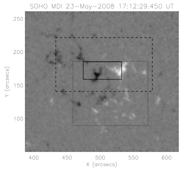
Figure 1.: The full fields of view of SOT/SP (dashed rectangle) and THEMIS/MTR (dotted rectangle). The solid rectangle denotes the region that we select to study the magnetic field in detail. The background is part of the full disk 96 min magnetogram observed by SOHO/MDI.fig01

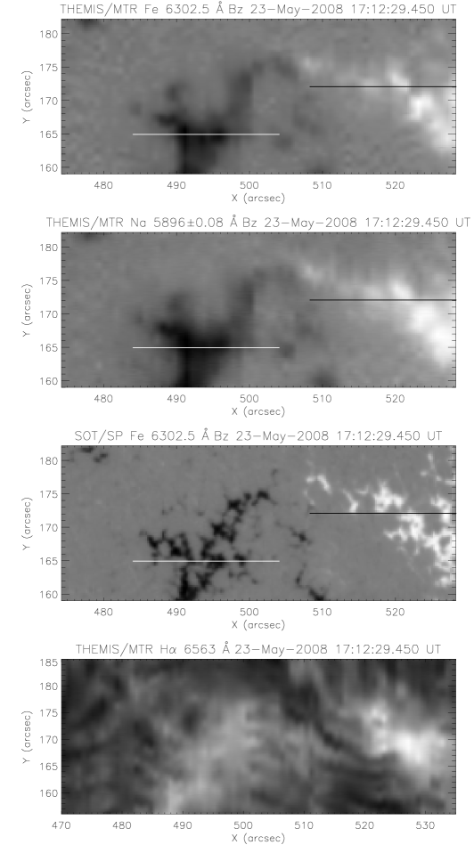
Figure 2.: LOS magnetic fields of THEMIS/MTR Fe i 6302.5 Å, Na D₁ 5896$\pm$0.8 Å, and SOT/SP Fe i 6302.5 Å in the solid rectangle region as shown in Figure fig01. The H$\alpha$ intensity map is shown in the bottom panel. Some slices are drawn and denoted by the solid lines on the magnetic field images, which will be used in Figures fig06 and fig08.fig02

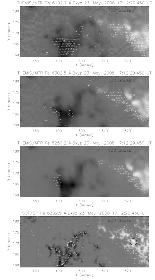
Figure 3.: The vector magnetic fields of THEMIS/MTR Ca i 6102.7 Å, Fe i 6302.5 Å, Fe i 5250.2 Å, and SOT/SP Fe i 6302.5 Å in the solid rectangle region as shown in Figure fig01. The 180^∘ ambiguity has been removed by the non-potential magnetic field calculation method and the fields have been transformed into the heliographic coordinates. Backgrounds are the vertical fields, white (black) is positive (negative). Arrows are the horizontal fields. The threshold of the plotted arrows is 50 gauss. The circles in the bottom panel denote the regions of divergence and convergence of the arrows.fig03

Figure 4.: Histograms of the product of field strengths and filling factors, the azimuth, and inclination angles in the regions as shown in Figure fig02 in the heliographic coordinates system. Only the fields where the field strength is greater than 50 gauss are included. The azimuth angles are measured counterclockwise from the north direction viewed towards the Sun and the 180^∘ ambiguity has been removed. The inclination angles are referred to the vertical direction of the solar surface. $0^{\circ}$ is away from the Sun center and $180^{\circ}$ is towards the Sun center.fig04

Figure 5.: The scatter plots show the comparisons of $B_{z}$, $B_{x}$, and $B_{y}$ obtained by UNNOFIT and MELANIE inversions and SOT/SP observation in the field of view of the solid rectangle shown in Figure fig01.fig05

Figure 6.: LOS magnetic field distribution along the white cut (left column) and along the black cut (right column) observed by SOT/SP (solid line) and MTR (dashed line). Top panels display the fields obtained by the inversion of the original SOT/SP observed profiles, while in the bottom row the Stokes profiles were convolved by a $3^{\prime\prime}\times 3^{\prime\prime}$ 2D boxcar function at each wavelength before inversion. See text for details. fig06

Figure 7.: Scatter plots of the LOS magnetic fields obtained by THEMIS/MTR Fe 6302.5 Å vs. Fe 5250.2 Å (left panel) and by MTR Fe 6302.5 Å vs. Ca 6102.7 Å (right panel). The data points are in the field of view of the solid rectangle shown in Figure fig01.fig07

Figure 8.: LOS magnetic fields along the white (left column) and black (right column) cuts as shown in Figure fig02. Top row shows the distributions for Ca i 6102.7 Å (dotted), Fe i 6302.5 Å (dashed), and Fe i 5250.2 Å (dash-dotted). Bottom row shows for Na D₁ 5896 Å with $\Delta\lambda=$ 0.08 Å (solid), 0.16 Å (dotted), 0.24 Å (dashed), and 0.32 Å (dash-dotted).fig08

Figure 9.: The sketch of a flux tube model and the parameters for the flux tube. $I_{\mathrm{m}}$, $V_{\mathrm{m}}$, and $B_{\mathrm{m}}$ are the Stokes parameters and LOS magnetic field at the flux tube center. $I$, $V$, and $B$ are the observed parameters convolved with the quiet sun region. The intensity of the quiet sun is $I_{\mathrm{q}}$. The half-widths of the tube and the spatial resolution are denoted by $\mathrm{w}_{\Delta\lambda}$ and $s$, respectively. All the parameters except $s$ depend on the wavelength position $\Delta\lambda$ from the line center of Na D₁ 5896 Å. Left and right panels show observations at the edge and at the center of the flux tubes, respectively.fig09

Table 1.: Instrumental characteristics for different lines of THEMIS/MTR and Hinode SOT/SP. The data were observed on 23 May 2008.tbl11

Line	Scan duration	Dispersion	Pixel size
	(UT)	(Å/pixel)	(arcsec)
MTR Ca i 6102.7 Å	16:44:03 – 17:38:55	0.0130	0.800, 0.236
MTR Fe i 6302.5 Å	16:44:03 – 17:38:55	0.0125	0.800, 0.233
MTR Fe i 5250.2 Å	16:44:03 – 17:38:55	0.0111	0.800, 0.230
MTR Na D1 5895.9 Å	16:44:03 – 17:38:55	0.0130	0.800, 0.232
MTR H$\alpha$ 6562.8 Å	16:44:03 – 17:38:55	0.0144	0.800, 0.226
SOT/SP Fe i 6302.5 Å	14:30:05 – 15:01:38	0.0215	0.297, 0.320

Table 2.: The free parameters fitted in UNNOFIT and MELANIE.tbl12

UNNOFIT	MELANIE
Zeeman splitting $\Delta\lambda_{\mathrm{H}}$	Field strength $B$
Inclination angle $\psi$	Inclination angle $\psi$
Azimuth angle $\phi$	Azimuth angle $\phi$
Line strength $\eta_{0}$	Line strength $\eta_{0}$
Doppler width $\Delta\lambda_{\mathrm{D}}$	Doppler width $\Delta\lambda_{\mathrm{D}}$
Damping parameter $\gamma$	Damping constant $a$
Line wavelength $\lambda_{0}$	Doppler velocity $v$
Parameter of source function $b$	Source function gradient $B_{1}$
Filling factor $\alpha$	Stray light fraction $f$
	Macro-turbulence velocity $v_{\mathrm{m}}$

Table 3.: Formation heights at the line center of Fe i 6302.5 Å and Fe i 5250.2 Å. The heights are measured from $\tau_{5000}=1$.tbl13

Method	Formation height (km)		Atmosphere model
	Fe i 6302.5 Å	Fe i 5250.2 Å
Bommier et al. (2007)	262	210	Maltby et al. (1986)
Bruls et al. (1991)	232	259	VAL-C
Sheminova (1998)	404	440	Holweger-Müller

Acknowledgements

THEMIS is a French–Italian telescope operated by the CNRS and CNR on the island of Tenerife in the Spanish Observatorio del Teide of the Instituto de Astrofísica de Canarias. Hinode is a Japanese mission developed and launched by ISAS/JAXA, with NAOJ as domestic partner and NASA and STFC (UK) as international partners. It is operated by these agencies in cooperation with ESA and NSC (Norway). The authors thank P. Mein, M.K. Georgoulis, N. Vitas, and T. T$\mathrm{\ddot{o}r\ddot{o}}$k very much for their help and discussions. Y. Guo was supported by the scholarship granted by China Scholarship Council (CSC) under file No. 2008619058. S. Gosain acknowledges CEFIPRA funding for his visit to Observatoire de Paris, Meudon, France under its project No. 3704-1.

References

- Berlicki, Mein, and Schmieder (2006) Berlicki, A., Mein, P., Schmieder, B.: 2006, A&A 445, 1127.
- Bommier and Molodij (2002) Bommier, V., Molodij, G.: 2002, A&A 381, 241.
- Bommier and Rayrole (2002) Bommier, V., Rayrole, J.: 2002, A&A 381, 227.
- Bommier, Rayrole, and Eff-Darwich (2005) Bommier, V., Rayrole, J., Eff-Darwich, A.: 2005, A&A 435, 1115.
- Bommier et al. (2007) Bommier, V., Landi Degl’Innocenti, E., Landolfi, M., Molodij, G.: 2007, A&A 464, 323.
- Bruls, Lites, and Murphy (1991) Bruls, J.H.M.J., Lites, B.W., Murphy, G.A.: 1991, In: November, L. (ed.) Solar Polarimetry, Proc. 11th Sacramento Peak Workshop, NSO, Sunspot, New Mexico, 444.
- Chae (2001) Chae, J.: 2001, ApJ 560, L95.
- Crouch, Barnes, and Leka (2009) Crouch, A.D., Barnes, G., Leka, K.D.: 2009, Sol. Phys. 260, 271. doi:10.1007/s11207-009-9454-2.
- Daras-Papamargaritis and Koutchmy (1983) Daras-Papamargaritis, H., Koutchmy, S.: 1983, A&A 125, 280.
- Georgoulis (2005) Georgoulis, M.K.: 2005, ApJ 629, L69.
- Guo et al. (2009) Guo, Y., Ding, M.D., Jin, M., Wiegelmann, T.: 2009, ApJ 696, 1526.
- Hasan and van Ballegooijen (2008) Hasan, S.S., van Ballegooijen, A.A.: 2008, ApJ 680, 1542.
- Holweger and Müller (1974) Holweger, H., Müller, E.A.: 1974, Sol. Phys. 39, 19.
- Ichimoto et al. (2008) Ichimoto, K., Lites, B., Elmore, D., Suematsu, Y., Tsuneta, S., Katsukawa, Y., Shimizu, T., Shine, R., Tarbell, T., Title, A., Kiyohara, J., Shinoda, K., Card, G., Lecinski, A., Streander, K., Nakagiri, M., Miyashita, M., Noguchi, M., Hoffmann, C., Cruz, T.: 2008, Sol. Phys. 249, 233.
- Ishikawa et al. (2008) Ishikawa, R., Tsuneta, S., Ichimoto, K., Isobe, H., Katsukawa, Y., Lites, B.W., et al.: 2008, Astron. Astrophys. Lett. 481, L25.
- Jefferies, Lites, and Skumanich (1989) Jefferies, J., Lites, B.W., Skumanich, A.: 1989, ApJ 343, 920.
- Keller et al. (2004) Keller, C.U., Schüssler, M., Vögler, A., Zakharov, V.: 2004, ApJ 607, L59.
- Kosugi et al. (2007) Kosugi, T., Matsuzaki, K., Sakao, T., Shimizu, T., Sone, Y., Tachikawa, S., et al.: 2007, Sol. Phys. 243, 3.
- Landolfi and Landi Degl’Innocenti (1982) Landolfi, M., Landi Degl’Innocenti, E.: 1982, Sol. Phys. 78, 355.
- Lites et al. (2007) Lites, B., Socas-Navarro, H., Kubo, M., Berger, T.E., Frank, Z., Shine, R.A., et al.: 2007, PASJ 59, 571.
- López Ariste, Rayrole, and Semel (2000) López Ariste, A., Rayrole, J., Semel, M.: 2000, A&AS 142, 137.
- Maltby et al. (1986) Maltby, P., Avrett, E.H., Carlsson, M., Kjeldseth-Moe, O., Kurucz, R.L., Loeser, R.: 1986, ApJ 306, 284.
- Mein et al. (2007) Mein, P., Mein, N., Faurobert, M., Aulanier, G., Malherbe, J.M.: 2007, A&A 463, 727.
- Metcalf et al. (2006) Metcalf, T.R., Leka, K.D., Barnes, G., Lites, B.W., Georgoulis, M.K., Pevtsov, A.A., et al.: 2006, Sol. Phys. 237, 267.
- Müller (1994) Müller, R.: 1994, In: Rutten, R.J., Schrijver, C.J. (eds.) Solar Surface Magnetism, Proc. NATO Advanced Research Workshop 433, Kluwer Academic Publishers, Dordrecht, 55.
- Nagata et al. (2008) Nagata, S., Tsuneta, S., Suematsu, Y., Ichimoto, K., Katsukawa, Y., Shimizu, T., et al.: 2008, ApJ 677, L145.
- Rachkovsky (1962) Rachkovsky, D.N.: 1962, Izv. Krymskoi Astrofiz. Obs. 27, 148.
- Scherrer et al. (1995) Scherrer, P.H., Bogart, R.S., Bush, R.I., Hoeksema, J.T., Kosovichev, A.G., Schou, J., et al.: 1995, Sol. Phys. 162, 129.
- Semel (1967) Semel, M.: 1967, Ann. Astrophys. 30, 513.
- Sheminova (1998) Sheminova, V.A.: 1998, A&A 329, 721.
- Shimizu et al. (2008) Shimizu, T., Nagata, S., Tsuneta, S., Tarbell, T., Edwards, C., Shine, R., et al.: 2008, Sol. Phys. 249, 221.
- Skumanich and Lites (1987) Skumanich, A., Lites, B.W.: 1987, ApJ 322, 473.
- Socas-Navarro (2001) Socas-Navarro, H.: 2001, In: Sigwarth, M. (ed.) Advanced Solar Polarimetry – Theory, Observation, and Instrumentation, ASP Conf. Ser. 236, 487.
- Stenflo (1973) Stenflo, J.O.: 1973, Sol. Phys. 32, 41.
- Strous (1994) Strous, L.H.: 1994, In: Rutten, R.J., Schrijver, C.J. (eds.) Solar Surface Magnetism, Proc. NATO Advanced Research Workshop 433, Kluwer Academic Publishers, Dordrecht, 73.
- Suematsu et al. (2008) Suematsu, Y., Tsuneta, S., Ichimoto, K., Shimizu, T., Otsubo, M., Katsukawa, Y., et al.: 2008, Sol. Phys. 249, 197.
- Tsuneta et al. (2008) Tsuneta, S., Ichimoto, K., Katsukawa, Y., Nagata, S., Otsubo, M., Shimizu, T., et al.: 2008, Sol. Phys. 249, 167.
- Unno (1956) Unno, W.: 1956, PASJ 8, 108.
- Vernazza, Avrett, and Loeser (1981) Vernazza, J.E., Avrett, E.H., Loeser, R.: 1981, ApJS 45, 635.
- Zwaan (1987) Zwaan, C.: 1987, ARA&A 25, 83.