Lowering the Error Floor of LDPC Codes Using Cyclic Liftings

Abstract

Cyclic liftings are proposed to lower the error floor of low-density parity-check (LDPC) codes. The liftings are designed to eliminate dominant trapping sets of the base code by removing the short cycles which form the trapping sets. We derive a necessary and sufficient condition for the cyclic permutations assigned to the edges of a cycle $c$ of length $\ell(c)$ in the base graph such that the inverse image of $c$ in the lifted graph consists of only cycles of length strictly larger than $\ell(c)$. The proposed method is universal in the sense that it can be applied to any LDPC code over any channel and for any iterative decoding algorithm. It also preserves important properties of the base code such as degree distributions, encoder and decoder structure, and in some cases, the code rate. The proposed method is applied to both structured and random codes over the binary symmetric channel (BSC). The error floor improves consistently by increasing the lifting degree, and the results show significant improvements in the error floor compared to the base code, a random code of the same degree distribution and block length, and a random lifting of the same degree. Similar improvements are also observed when the codes designed for the BSC are applied to the additive white Gaussian noise (AWGN) channel.

I Introduction

Low-density parity-check (LDPC) codes [8] have emerged as one of the top contenders for capacity approaching error correction over many important channels. They not only perform superbly but also lend themselves well to highly efficient parallel decoding algorithms. A well-known construction of LDPC codes is based on protographs, also referred to as base graphs or projected graphs [15]. In such constructions, a bipartite base graph $G$ is copied $N$ times and for each edge $e$ of $G$, a permutation is applied to the $N$ copies of $e$ to interconnect the $N$ copies of $G$. The resulting graph, called the $N$-cover or the $N$-lifting of $G$, is then used as the Tanner graph [17] of the LDPC code. If the permutations are cyclic, the resulting LDPC code is called quasi-cyclic (QC). QC LDPC codes are attractive due to their simple implementation and analysis [15].

At very large block lengths, the performance of LDPC codes can be well estimated using asymptotic techniques such as density evolution [14]. At finite lengths, however, our understanding of the dynamics of iterative decoding algorithms is limited. In particular, iteratively decoded finite-length codes demonstrate an abrupt change in their error rate curves, referred to as error floor, in the high signal to noise ratio (SNR) region. The analysis of the error floor and techniques to improve the error floor performance of LDPC codes are still very active areas of research. For the binary erasure channel (BEC), the error floor is well understood and is known to be caused by graphical structures called stopping sets [5]. Richardson related the error rate performance of LDPC codes on the binary symmetric channel (BSC) and the additive white Gaussian noise (AWGN) channel to more general graphical structures, called trapping sets, and devised a technique to estimate the error floor [13]. Other estimation techniques based on finding the dominant trapping sets were also proposed for the BSC in [3] and for the AWGN channel in [4], [16]. In [22] - [24], Xiao and Banihashemi took a different approach, and instead of focusing on trapping sets which are the eventual result of the decoder failure, focussed on the input error patterns that cause the decoder to fail. A simple technique for estimating the frame error rate (FER) and the bit error rate (BER) of finite-length LDPC codes over the BSC was developed in [22]. The complexity of this algorithm was then reduced in [24], and the estimation technique was extended to the AWGN channel with quantized output in [23]. More recent work on the estimation of the error floor of LDPC codes is presented in [2], [6], to which the reader is also referred for a more comprehensive list of references.

There is extensive literature on reducing the error floor of finite-length LDPC codes over different channels and for different iterative decoding algorithms. One category of such literature, focusses on modification of iterative decoding algorithms, see, e.g., [9], while another category is concerned with the code construction. In the second category, some researchers use indirect measures such as girth [18] or approximate cycle extrinsic message degree (ACE) [19], while others work with direct measures of error floor performance such as the distribution of stopping sets or trapping sets [20], [10], [11]. In [20], edge swapping is proposed as a technique to increase the stopping distance of an LDPC code, and thus to improve its error floor performance over the BEC. Random cyclic liftings are also studied in [20] and shown to improve the average performance of the ensemble in the error floor region compared to the base code. Ivkovic et al. [10] apply the same technique of edge swapping between two copies of a base LDPC code to eliminate the dominant trapping sets of the base code over the BSC.

In the approach proposed here also, we focus on dominant trapping sets which are the main contributors to the error floor. We start from the code whose error floor is to be improved, as the base code. We then construct a new code by cyclically lifting the base code. The lifting is designed carefully to eliminate the dominant trapping sets of the base graph. This is achieved by removing the short cycles which form the dominant trapping sets. Our work has similarities to [10] and [20]. The similarity with both [10] and [20] is that we also use graph covers or liftings to improve the error floor performance of a base code. It however differs from [10] in that we restrict ourselves to cyclic liftings that are advantageous in implementation. Moreover, to eliminate the dominant trapping sets we use a different approach than the one in [10]. More specifically, our approach is based on the elimination of the short cycles involved in the trapping sets. To do so, we derive a necessary and sufficient condition for the problematic cycles of the base code such that they are mapped to strictly larger cycles in the lifted code. The difference with [20] is that while [20] is focused on the ensemble performance of random liftings, our work is concerned with the intentional design of a particular cyclic lifting.

Given a base code and its dominant trapping sets over a certain channel and under a specific iterative decoding algorithm, the proposed construction can lower the error floor by increasing the block length while preserving the important properties of the base code such as degree distributions, and the encoder and decoder structure. The code rate is also preserved or is decreased slightly depending on the rank deficiency of the parity-check matrix of the base code. Moreover, the cyclic nature of the lifting makes it implementation friendly. We apply the proposed construction to the Tanner code [18] and two randomly constructed codes, one regular and the other irregular, to improve the error floor performance of Gallager A/B algorithms over the BSC. Simulation results show a consistent improvement in the error floor performance by increasing the degree of liftings. The constructed codes are far superior to similar random codes or codes constructed by random liftings in the error floor region. We also examine the performance of the codes constructed for BSC/Gallager B algorithm, over the AWGN channel with min-sum decoding and observe similar improvements in the error floor performance.

The remaining of the paper is organized as follows: Section II introduces definitions, notations and background material used throughout the paper. In Section III, the proposed construction is explained and discussed. Numerical results are presented in Section IV, and finally Section V concludes the paper.

II PRELIMINARIES: LDPC CODES, TANNER GRAPHS, GRAPH LIFTINGS AND TRAPPING SETS

II-A LDPC Codes and Tanner Graphs

Consider a binary LDPC code ${\cal C}$ represented by a Tanner graph $G=(V_{b}\cup V_{c},E)$, where $V_{b}=\{b_{1},\ldots,b_{n}\}$ and $V_{c}=\{c_{1},\ldots,c_{m}\}$ are the sets of variable nodes and check nodes, respectively, and $E$ is the set of edges. Corresponding to $G$, we have an $m\times n$ parity-check matrix $H=[h_{ij}]$ of ${\cal C}$, where $h_{ij}=1$ if and only if (iff) the node $c_{i}\in V_{c}$ is connected to the node $b_{j}\in V_{b}$ in $G$; or equivalently, iff $\{b_{j},c_{i}\}\in E$. If all the nodes in the set $V_{b}$ have the same degree $d_{v}$ and all the nodes in the set $V_{c}$ have the same degree $d_{c}$, the corresponding LDPC code is called a regular $(d_{v},d_{c})$ code. Otherwise, it is called irregular.

A subgraph of $G$ is a path of length $k$ if it consists of a sequence of $k+1$ nodes $\{u_{1},\ldots,u_{k+1}\}$ and $k$ distinct edges $\{\{u_{i},u_{i+1}\}:i=1,\ldots,k\}$. We say two nodes are connected if there is a path between them. A path is a cycle if $u_{1}=u_{k+1}$, and all the other nodes are distinct. The length of the shortest cycle(s) in the graph is called girth. In bipartite graphs, including Tanner graphs, all cycles have even lengths. So, the girth is an even number.

II-B Graph Liftings

Consider the set of all possible permutations $S_{N}$ over the set of integer numbers $Z_{1\rightarrow N}\stackrel{{\scriptstyle\Delta}}{{=}}\{1,\ldots,N\}$. This set forms a group, known as the symmetric group, under composition. Each element $\pi\in S_{N}$ can be represented by all the values $\pi(i),\>i\in Z_{1\rightarrow N}$. For the identity element $\pi_{0}$, we have $\pi_{0}(i)=i,\forall i$, and the inverse of $\pi$ is denoted by $\pi^{-1}$ and defined as $\pi^{-1}(\pi)=\pi_{0}$. It is easy to see that the symmetric group is not Abelian. An alternate representation of permutations is to represent a permutation $\pi$ with an $N\times N$ matrix $\Pi=[\pi_{ij}]$, whose elements are defined by $\pi_{ij}=1$ if $j=\pi(i)$, and $\pi_{ij}=0$, otherwise. As a result, we have the isomorphic group of all $N\times N$ permutation matrices with the group operation defined as matrix multiplication, and the identity element equal to the identity matrix $I_{N}$. In particular, corresponding to the composition $\pi^{\prime}(\pi)$, we have the matrix multiplication $\Pi\times\Pi^{\prime}$. Moreover, since the permutation matrices are orthogonal, the inverse of a permutation matrix is its transpose, i.e., $\Pi^{-1}=\Pi^{T}$.

Consider the cyclic subgroup $C_{N}$ of $S_{N}$ consisting of the $N$ circulant permutations defined by $\pi_{d}(i)=i+d\>\>\>\;\mbox{mod}\>\>\>\;N+1,\>d\in Z_{0\rightarrow N-1}$. The permutation $\pi_{d}$ corresponds to $d$ cyclic shifts to the right. In the matrix representation, permutation $\pi_{d}$ corresponds to a permutation matrix whose rows are obtained by cyclically shifting all the rows of the identity matrix $I_{N}$ by $d$ to the right. This matrix is denoted by $I^{(d)}$. Note that $I^{(0)}=I_{N}$. For the composition of permutations, we have

$$I^{(d_{1})}\times I^{(d_{2})}=I^{(d_{1}+d_{2}\>\mbox{mod}\;N)}\>.$$ (1)

Clearly, $C_{N}$ can be generated by $I^{(1)}$, where each element $I^{(d)},\>d\in Z_{0\rightarrow N-1}$ of $C_{N}$ is the $d$-th power of $I^{(1)}$. This defines a natural isomorphism between $C_{N}$ and the set of integers modulo $N$, $Z_{0\rightarrow N-1}$, under addition. The latter group is denoted by $Z_{N}$.

Consider the following construction of a graph $\tilde{G}=(\tilde{V},\tilde{E})$ from a graph $G=(V,E)$: We first make $N$ copies of $G$ such that for each node $v\in V$, we have $N$ copies $\tilde{v}\stackrel{{\scriptstyle\Delta}}{{=}}\{v_{1}\ldots,v_{N}\}$ in $\tilde{V}$. For each edge $e=\{u,v\}\in E$, we assign a permutation $\pi^{e}\in S_{N}$ to the $N$ copies of $e$ in $\tilde{E}$ such that an edge $\{u_{i},v_{j}\}$ belongs to $\tilde{E}$ iff $\pi^{e}(i)=j$. The set of these edges is denoted by $\tilde{e}$. The graph $\tilde{G}$ is called an $N$-cover or an $N$-lifting of $G$, and $G$ is referred to as the base graph, protograph or projected graph corresponding to $\tilde{G}$. We also call the application of a permutation $\pi^{e}$ to the $N$ copies of $e$, edge swapping, high lighting the fact that the permutation swaps edges among the $N$ copies of the base graph.

In this work, $G$ is a Tanner graph, and we define the edge permutations from the variable side to the check side, i.e., the set of edges $\tilde{e}$ in $\tilde{E}$ corresponding to an edge $e=\{b,c\}\in E$ are defined by $\{b_{i},c_{\pi^{e}(i)}\},\>i\in Z_{1\rightarrow N}$. Equivalently, $\tilde{e}$ can be described by $\{b_{(\pi^{e})^{-1}(j)},c_{j}\},\>j\in Z_{1\rightarrow N}$. Our focus in this paper is on cyclic liftings of $G$, where the edge permutations are selected from $C_{N}$, or equivalently $Z_{N}$. Thus the nomenclature cyclic edge swapping. In this case, if $I^{(d)}$ is a permutation matrix from variable nodes to check nodes, $I^{(d^{\prime})};\>d^{\prime}=N-d\>\>\mbox{mod}\>\>N$, will be the corresponding permutation matrix from check nodes to variable nodes. It is important to distinguish between the two cases when we compose permutations on a directed path.

To the lifted graph $\tilde{G}$, we associate an LDPC code $\tilde{\cal{C}}$, referred to as the lifted code, such that the $mN\times nN$ parity-check matrix $\tilde{H}$ of $\tilde{\cal{C}}$ is equal to the adjacency matrix of $\tilde{G}$. More specifically, $\tilde{H}$ consists of $m\times n$ sub-matrices $[\tilde{H}]_{ij}\>,1\leq i\leq m,\>1\leq j\leq n$, arranged in $m$ rows and $n$ columns. The sub-matrix $[\tilde{H}]_{ij}$ in row $i$ and column $j$ is the permutation matrix from $C_{N}$ corresponding to the edge $\{b_{j},c_{i}\}$ where $h_{ij}\neq 0$; otherwise, $[\tilde{H}]_{ij}$ is the all-zero matrix. Let the $m\times n$ matrix $D=[d_{ij}]$ be defined by $[\tilde{H}]_{ij}=I^{(d_{ij})},\>d_{ij}\in Z_{N}$ if $h_{ij}\neq 0$, and $d_{ij}=+\infty$, otherwise. Matrix $D$, called the matrix of edge permutation indices, fully describes $\tilde{H}$ and thus the cyclically lifted code $\tilde{\cal{C}}$.

II-C Trapping Sets and Error Floor

It is well-known that trapping sets are the culprits in the error floor region of iterative decoding algorithms. An $(a,b)$ trapping set is defined as a set of $a$ variable nodes which have $b$ check nodes of odd degree in their induced subgraph. Among trapping sets, the most harmful ones are called dominant. Trapping sets depend not only on the Tanner graph of the code but also on the channel and the iterative decoding algorithm. In general, finding all the trapping sets is a hard problem, and one often needs to resort to efficient search techniques to obtain the dominant trapping sets [13], [4], [24], [21]. Trapping sets for Gallager A/B algorithms over the BSC are examined for a number of LDPC codes in [3], [24]. In this work, we assume that the dominant trapping sets are known and available.

In the context of symmetric decoders over the BSC, the error floor of FER can be estimated by [22]

$$FER\approx N_{J}\>\epsilon^{J}\>,$$ (2)

where $\epsilon$ is the channel crossover probability, and $J$ and $N_{J}$ are the size and the number of the smallest error patterns that the decoder fails to correct. From (2), it is clear that the dominant trapping sets over the BSC are those caused by the minimum number of initial errors. (In [3], [10], parameter $J$ in (2) is called minimum critical number.) In the double-logarithmic plane, one can see from (2) that $\log(FER)$ decreases linearly with $\log(\epsilon)$ and the slope of the line is determined by $J$.

III DESIGN OF CYCLIC LIFTINGS TO ELIMINATE TRAPPING SETS

In this work, our focus is on the design of cyclic liftings of a given Tanner graph to eliminate its dominant trapping sets with respect to a given channel/decoding algorithm with the purpose of reducing the error floor. (This is equivalent to the design of non-infinity edge permutation indices of matrix $D$.) For example, Equation (2) indicates that for improving the error floor on the BSC, one needs to increase $J$ and decrease $N_{J}$ corresponding to the dominant trapping sets. In particular, while increasing $J$ for dominant trapping sets increases the slope of $\log(\mbox{FER})$ vs. $\log(\epsilon)$ at low channel crossover probabilities $\epsilon$, reducing $N_{J}$ amounts to a downward shift of the curve. So, the general idea is to primarily increase $J$ by eliminating the trapping sets with the smallest critical number, and the secondary goal is then to decrease $N_{J}$.

It is well-known that dominant trapping sets composed of short cycles [3], [24]. To eliminate the trapping sets, we thus aim at eliminating their constituent cycles in the lifted graph. In the following, we examine the inverse image of a (base) cycle in the cyclically lifted graph.

III-A Cyclic Liftings of Cycles

Lemma 1

Consider a cyclic $N$-lifting $\tilde{G}$ of a Tanner graph $G$. Consider a path $\xi$ of length $\ell$ in $G$, which starts from a variable node $b$ and ends at a variable node $b^{\prime}$ with the sequence of edges $e_{1},\ldots,e_{\ell}$. Corresponding to the edges, we have the sequence of permutation matrices $I^{(d_{1})},\ldots,I^{(d_{\ell})}$. Then the permutation matrix that maps $\tilde{b}$ to $\tilde{b^{\prime}}$ through the path $\tilde{\xi}$ is $I^{(d)}$, where

$$d=\sum_{i=0}^{\ell-1}(-1)^{i}d_{i+1}\>\mbox{mod}\>N\>.$$ (3)

Proof:

The permutation matrix that maps $\tilde{b}$ to $\tilde{b^{\prime}}$ is obtained by multiplying the permutation matrices of the “directed" edges along the path. This results in $I^{(d)}=I^{(d_{1})}\times I^{(N-d_{2}\>\mbox{mod}\>N)}\times\cdots\times I^{(N-d_{\ell}\>\mbox{mod}\>N)}$. The lemma is then proved using (1). ∎

The value of $d$ given in (3) is called the permutation index of the path from $b$ to $b^{\prime}$. Clearly, the permutation index of the path from $b^{\prime}$ to $b$ is equal to $d^{\prime}=N-d\>\>\mbox{mod}\>\>N$. If $b=b^{\prime}$ and all the other nodes are distinct, then the path will become a cycle and depending on the direction of the cycle, its permutation index will be equal to $d$ or $d^{\prime}$.

Theorem 1

Consider the cyclic $N$-lifting $\tilde{G}$ of the Tanner graph $G$. Suppose that $c$ is a cycle of length $\ell$ in $G$. The inverse image of $c$ in $\tilde{G}$ is then the union of $N/k$ cycles, each of length $k\ell$, where $k$ is the order of the element(s) of $Z_{N}$ corresponding to the permutation indices of $c$.

Proof:

We first note that the elements of $Z_{N}$ corresponding to both permutation indices of $c$ have the same order. Suppose that the permutation indices of $c$ in the two directions are equal to $d$ and $d^{\prime}=N-d\>\>\mbox{mod}\>\>N$. Now, $d^{\prime}$ is the inverse of $d$ in $Z_{N}$, and thus has the same order as $d$.

Denote the sequence of variable and check nodes in $c$ by $b_{i_{1}},c_{i_{2}},b_{i_{3}},c_{i_{4}},\ldots,b_{i_{\ell-1}},c_{i_{\ell}},b_{i_{1}}$. Starting from any of the $N$ variable nodes in $\tilde{b_{i_{1}}}$, say $b_{i_{1}j},\>1\leq j\leq N$, without loss of generality, we follow one of the two paths of length $\ell$ in the inverse image of $c$ in $\tilde{G}$, which corresponds to the direction on $c$ associated with the permutation index $d$. As a result, based on Lemma 3, we will end up at the variable node $b_{i_{1}p}$ in $\tilde{b_{i_{1}}}$, where $p=j+d\>\>\>\mbox{mod}\>\>\>N$ and $d$ is given in (3). If $d=0$, then the path ends at $b_{i_{1}j}$, meaning that the inverse image of $c$ which passes through $b_{i_{1}j}$ is a cycle of length $\ell$. Similarly one can see that the inverse image of $c$ passing through any of the $N$ nodes $b_{i_{1}1},\ldots,b_{i_{1}N}$ is a cycle of length $\ell$, and since these cycles do not overlap, the inverse image of $c$ in this case is the union of $N$ cycles, each of length $\ell$. This corresponds to the case where the element of $Z_{N}$ corresponding to the permutation index of $c$ is $0$, which has order $k=1$. For the cases where $d\neq 0$, continuing along the path and passing through $q\ell$ edges of the inverse image of $c$, we reach the node $b_{i_{1}p^{\prime}}$, where $p^{\prime}=j+qd\>\>\>\mbox{mod}\>\>\>N$. Clearly, we will be back to the starting node for the first time when $qd=0\>\>\mbox{mod}\>\>N$, for the smallest value of $q$. (In that case by continuing the path we will just go over the same cycle of length $q\ell$.) By definition, $q$ is the order of $d$ in $Z_{N}$, and thus $q=k$. Since the order of any element of a finite group divides the order of the group, $s=N/k$ is an integer. It can then be easily seen that by starting from any of the nodes $b_{i_{1}1},\ldots,b_{i_{1}s}$, we can partition the inverse image of $c$ into $s$ cycles of length $k\ell$ each. This completes the proof. ∎

In what follows, we refer to the value $k$ in Theorem 1 as the order of cycle $c$, and use the notation ${\cal O}(c)$ to denote it.

Corollary 1

Consider the cyclic $N$-lifting $\tilde{G}$ of the Tanner graph $G$. Suppose that $c$ is a cycle of length $\ell$ in $G$. The inverse image of $c$ in $\tilde{G}$ is the union of non-overlapping cycles, each strictly longer than $\ell$ iff ${\cal O}(c)>1$; or equivalently, iff the permutation index of $c$, given in (3), is nonzero.

III-B Intentional Edge Swapping (IES) Algorithm

Suppose that $T$ is the set of all dominant trapping sets, and $C(T)$ is the set of all the cycles in $T$. We also use the notations $t$ and $C(t)$ for a trapping set and its constituent cycles, respectively. For an edge $e$, we use $C^{e}(t)$ to denote the set of cycles in the trapping set $t$ that include $e$. In the previous subsection, we proved that a cycle $c$ in the base Tanner graph $G$ is mapped to the union of larger cycles in the cyclically lifted graph $\tilde{G}$ iff ${\cal O}(c)>1$. To eliminate the dominant trapping sets, we are thus interested in assigning the edge permutation indices to the edges of $C(T)$ such that ${\cal O}(c)>1$ for every cycle $c\in C(T)$. To achieve this, we order the trapping sets in accordance with the increasing order of their critical number. We still denote this ordered set by $T$ with a slight abuse of notation. Note that $T$ may now include trapping sets with critical numbers larger than the minimum one. We then go through the trapping sets in $T$ one at a time and identify and list all the cycles involved in each trapping set in $C(T)$, i.e., $C(T)=\{c\in C(t),\forall t\in T\}$. Note that $C(T)$ is also partially ordered based on the corresponding ordering of the trapping sets in $T$.

Example 1

Three typical trapping sets for Gallager A/B algorithms are shown in Fig. 1 [3]. The $(4,4)$ and $(5,3)$ trapping sets include one and three cycles of length 8, respectively, while the $(4,2)$ trapping set has 2 cycles of length 6 and one cycle of length 8.

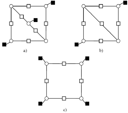
Figure 1: a) (5, 3) Trapping set b) (4, 2) Trapping set c) (4, 4) Trapping set. $\circ=$ Variable Node, $\square=$ Even degree Check Node and $\blacksquare=$ Odd degree Check Node.

The next step is to choose proper edges of each trapping set to be swapped, i.e., to choose the edges to which nonzero permutation indices are assigned. In general, the policy is to select the minimum number of edges that can result in ${\cal O}(c)>1$ for every cycle $c$ in the trapping set $t$ under consideration.

Example 2

Going back to Fig. 1, for the $(4,4)$ trapping set, it would be enough to just pick one of the edges of the cycle of length 8 to eliminate this cycle in the lifted graph. For the $(5,3)$ and $(4,2)$ trapping sets, however, at least two edges should be selected for the elimination of all the cycles. A proper choice would be to select one edge from the diagonal and the other edge from one of the sides.

Related to the edge selection, is the next step of permutation index assignment to the selected edges such that ${\cal O}(c)>1$ for every cycle $c\in C(t)$. In general, we would like to have larger orders for the cycles. This in turn would result in larger cycles in the lifted graph. To limit the complexity, however, we approach this problem in a greedy fashion and with the main goal of just eliminating all the cycles in $C(t)$, i.e., for each selected edge $e$, we choose the permutation index such that all the cycles $C^{e}(t)$ have orders larger than one. This can be performed by sequentially testing the values in the set $Z_{1\rightarrow N}$. As soon as such an index is found, we assign it to $e$ and move to the next selected edge and repeat the same process.

We call the proposed algorithm intentional edge swapping (IES) to distinguish it from “random edge swapping," commonly used to construct lifted codes and graphs. The pseudocode of the algorithm is given as Algorithm 1. At the output of Algorithm 1, we have the sets $SwappedSet$ and $IndexSet$, which contain the edges of the Tanner graph that should be swapped, and their corresponding permutation indices, respectively.

1) Initialization: Create the ordered sets $T$ and $C(T)$. Select $N$. $ProcessedSet=\emptyset$, $SwappedSet=\emptyset$, $IndexSet=\emptyset$.
2) Select the next trapping set $t\in T$.
3) $CurrentSet=$ edges of $C(t)$.
4) $CandidateSet=CurrentSet\setminus ProcessedSet$.
5) If $CandidateSet=\emptyset$, go to Step 8.
6) Select the edges ${\cal E}$ from $CandidateSet$ that should be swapped, and assign their permutation indices ${\cal I}$ from $Z_{1\rightarrow N}$ such that ${\cal O}(c)>1$ for every cycle $c$ in $C^{e}(t)$.
7) $SwappedSet=SwappedSet\>\cup\>{\cal E}$, $IndexSet=IndexSet\>\cup\>{\cal I}$, and $ProcessedSet=ProcessedSet\>\cup\>CurrentSet$. Go to Step 12.
8) $CandidateSet=CurrentSet\setminus SwappedSet$. If $CandidateSet=\emptyset$, Stop.
9) Select an edge $e$ from $CandidateSet$ and assign a permutation index $i\in Z_{1\rightarrow N}$ to it such that for all cycles $c\in C^{e}(ProcessedSet\>\cup\>t)$, we have ${\cal O}(c)>1$. If this is not feasible, go to Step 11.
10) $SwappedSet=SwappedSet\cup e$, $IndexSet=IndexSet\cup i$, and $CurrentSet=CurrentSet\setminus C^{e}(t)$. If $CurrentSet\neq\emptyset$, go to Step 8. Otherwise, go to Step 12.
11) $CandidateSet=CandidateSet\setminus e$, If $CandidateSet\neq\emptyset$, go to Step 9. Else, stop.
12) If all the trapping sets in $T$ are processed, stop. Otherwise, go to Step 2.

Algorithm 1 Intentional Edge Swapping (IES) Algorithm

In Algorithm 1, the search for edges to be swapped and the permutation index assignment to these edges are performed in two phases. The first phase is in Steps 4 - 6, where any edge from previously processed trapping sets is removed from the set of candidates for swapping. If the first phase fails, in that no edge exists as a candidate for swapping ($CandidateSet=\emptyset$), then the algorithm switches to the second phase in Steps 8 - 9, where only previously swapped edges are removed from the candidate set for swapping.

The process of permutation index assignment in Algorithm 1 involves the satisfaction of inequalities $d\neq 0$ for certain cycles, where $d$ is given in (3). In general, this is easier to achieve if the variables involved in (3) are selected from a larger alphabet space. In fact, by increasing $N$, one can eliminate more trapping sets and achieve a better performance in the error floor region.

III-C Minimum Distance and Rate of Cyclic Liftings

Consider an LDPC code $\cal{C}$ with an $m\times n$ parity-check matrix $H$. To prove our results on the minimum distance and the rate of a cyclic $N$-lifting $\tilde{\cal{C}}$ of $\cal{C}$, we consider an alternate parity-check matrix $\tilde{H}^{\prime}$ of $\tilde{\cal{C}}$ obtained by permutations of rows and columns of matrix $\tilde{H}$ introduced in Subsection II-B, as follows:

$${\tilde{H}^{\prime}}=\left(\begin{array}[]{cccccc}\mathcal{A}_{0}&\mathcal{A}_{N-1}&\mathcal{A}_{N-2}&\ldots&\mathcal{A}_{2}&\mathcal{A}_{1}\\ \mathcal{A}_{1}&\mathcal{A}_{0}&\mathcal{A}_{N-1}&\ldots&\mathcal{A}_{3}&\mathcal{A}_{2}\\ \vdots&\vdots&\vdots&\ddots&\vdots&\vdots\\ \mathcal{A}_{N-2}&\mathcal{A}_{N-3}&\mathcal{A}_{N-4}&\ldots&\mathcal{A}_{0}&\mathcal{A}_{N-1}\\ \mathcal{A}_{N-1}&\mathcal{A}_{N-2}&\mathcal{A}_{N-3}&\ldots&\mathcal{A}_{1}&\mathcal{A}_{0}\end{array}\right)\>.$$ (4)

In (4), all the sub matrices $\mathcal{A}_{d},\>d=0,\ldots,N-1$, have size $m\times n$, and are given by

$$(i,j)\text{th entry of }\mathcal{A}_{d}=\left\{\begin{array}[]{cc}1&\textrm{if $d=d_{ij}$}\\ 0&\quad\textrm{otherwise},\\ \end{array}\right.$$ (5)

where $d_{ij}$ is the permutation index corresponding to $h_{ij}$. The parity-check matrix $\tilde{H}^{\prime}$ is block circulant with the property that

$$\mathcal{A}_{0}+\mathcal{A}_{1}+\ldots+\mathcal{A}_{N-1}=H.$$ (6)

Theorem 2

If code $\cal{C}$ has rate $r$, then the rate $r^{(N)}$ of a cyclic $N$-lifting $\tilde{\cal{C}}$ of $\cal{C}$ satisfies $r^{(N)}\leq r$, for $N=2^{q},\>q=1,2,3,\ldots$.

Proof:

Due to the block circulant structure of $\tilde{H}^{\prime}$, it can be written as

$$\tilde{H}^{\prime}=\left(\begin{array}[]{c c}\mathcal{M}&\mathcal{N}\\ \mathcal{N}&\mathcal{M}\end{array}\right)\>,$$ (7)

where matrices $\mathcal{M}$ and $\mathcal{N}$ are given by

$$\mathcal{M}=\left(\begin{array}[]{ccccc}\mathcal{A}_{0}&\mathcal{A}_{N-1}&\ldots&\mathcal{A}_{\frac{N}{2}+2}&\mathcal{A}_{\frac{N}{2}+1}\\ \mathcal{A}_{1}&\mathcal{A}_{0}&\ldots&\mathcal{A}_{\frac{N}{2}+3}&\mathcal{A}_{\frac{N}{2}+2}\\ \vdots&\vdots&\ldots&\vdots&\vdots\\ \mathcal{A}_{\frac{N}{2}+1}&\mathcal{A}_{\frac{N}{2}}&\ldots&\mathcal{A}_{1}&\mathcal{A}_{0}\end{array}\right)_{\frac{N}{2}m\times\frac{N}{2}n},$$

and

$$\mathcal{N}=\left(\begin{array}[]{ccccc}\mathcal{A}_{\frac{N}{2}}&\mathcal{A}_{\frac{N}{2}-1}&\ldots&\mathcal{A}_{2}&\mathcal{A}_{1}\\ \mathcal{A}_{\frac{N}{2}+1}&\mathcal{A}_{\frac{N}{2}}&\ldots&\mathcal{A}_{3}&\mathcal{A}_{2}\\ \vdots&\vdots&\ldots&\vdots&\vdots\\ \mathcal{A}_{N-1}&\mathcal{A}_{N-2}&\ldots&\mathcal{A}_{\frac{N}{2}+3}&\mathcal{A}_{\frac{N}{2}+2}\end{array}\right)_{\frac{N}{2}m\times\frac{N}{2}n},$$

respectively. (Note that all indices $i$ of $\mathcal{A}_{i}$ should be interpreted as modulo $N$.) Adding the second block column of (7) to the first, followed by adding the first block row to the second, we have

$$\left(\begin{array}[]{c c}\mathcal{M}&\mathcal{N}\\ \mathcal{N}&\mathcal{M}\end{array}\right)\rightarrow\left(\begin{array}[]{c c}\mathcal{M}+\mathcal{N}&\mathcal{N}\\ \mathcal{N}+\mathcal{M}&\mathcal{M}\end{array}\right)\rightarrow\left(\begin{array}[]{c c}\mathcal{M}+\mathcal{N}&\mathcal{N}\\ 0&\mathcal{M}+\mathcal{N}\end{array}\right)\>.$$ (8)

For $N=2$, $\mathcal{M}+\mathcal{N}=H$, and since the rank of the matrix in (8), and thus the rank of $\tilde{H}^{\prime}$, is at least twice the rank of $H$, we have $r^{(2)}\leq r$, and the proof is complete. For $N>2$, it is easy to see that $\mathcal{M}+\mathcal{N}$ is also block circulant and can in turn be partitioned into four sub matrices, each of size $\frac{N}{4}m\times\frac{N}{4}n$, as follows:

$$\mathcal{M}+\mathcal{N}=\left(\begin{array}[]{c c}\mathcal{M}^{\prime}&\mathcal{N}^{\prime}\\ \mathcal{N}^{\prime}&\mathcal{M}^{\prime}\end{array}\right)\>.$$

Replacing this in the rightmost matrix of (8), and performing similar block operations as in (8), we obtain

$$\left(\begin{array}[]{c | c}\begin{array}[]{c c}\mathcal{M}^{\prime}&\mathcal{N}^{\prime}\\ \mathcal{N}^{\prime}&\mathcal{M}^{\prime}\end{array}&\mathcal{N}\\ \hline\cr 0&\begin{array}[]{c c}\mathcal{M}^{\prime}&\mathcal{N}^{\prime}\\ \mathcal{N}^{\prime}&\mathcal{M}^{\prime}\end{array}\end{array}\right)\rightarrow$$

$$\left(\begin{array}[]{c | c}\begin{array}[]{c c}\mathcal{M}^{\prime}+\mathcal{N}^{\prime}&\mathcal{N}^{\prime}\\ 0&\mathcal{M}^{\prime}+\mathcal{N}^{\prime}\end{array}&\mathcal{P}\\ \hline\cr 0&\begin{array}[]{c c}\mathcal{M}^{\prime}+\mathcal{N}^{\prime}&\mathcal{N}^{\prime}\\ 0&\mathcal{M}^{\prime}+\mathcal{N}^{\prime}\end{array}\end{array}\right)\>.$$ (9)

For $N=4$, $\mathcal{M}^{\prime}+\mathcal{N}^{\prime}=H$, and as the rank of the matrix in (9) is at least four times the rank of $H$, we have $r^{(4)}\leq r$, and the proof is complete. For $N=2^{q}>4$, the same process of block column and row operations is repeated $q$ times resulting in a block upper triangular matrix with the following structure

$$\left(\begin{array}[]{ccccc}H&\mathcal{B}_{1,2}&\ldots&\mathcal{B}_{1,N-1}&\mathcal{B}_{1,N}\\ 0&H&\ldots&\mathcal{B}_{2,N-1}&\mathcal{B}_{2,N}\\ \vdots&\vdots&\cdots&\vdots&\vdots\\ 0&0&\ldots&H&\mathcal{B}_{N-1,N}\\ 0&0&\ldots&0&H\end{array}\right)_{Nm\times Nn}\>.$$ (10)

As the rank of the above matrix, and thus the rank of $\tilde{H}^{\prime}$, is at least $N$ times the rank of $H$, we have $r^{(N)}\leq r$. ∎

Corollary 2

If matrix $H$ has full rank, then $r^{(N)}=r$, for $N=2^{q},\>q=1,2,3,\ldots$.

Proof:

If $H$ has full rank, then the matrix in (10) is also full-rank, and so is $\tilde{H}^{\prime}$. This implies $r^{(N)}=r$. ∎

It is easy to find counter examples to demonstrate that Theorem 2 and Corollary 2 do not always hold for odd values of $N$ or even values that are not integer powers of two.

Theorem 3

If code $\cal{C}$ has minimum distance $d_{min}$, then the minimum distance $d_{min}^{(N)}$ of a cyclic $N$-lifting $\tilde{\cal{C}}$ of $\cal{C}$ satisfies $d_{min}\leq d_{min}^{(N)}\leq N\;d_{min}$, for $N=2^{q},\>q=1,2,3,\ldots$.

Proof:

We first prove the lower bound. Consider a codeword $\underline{c}^{(N)}$ with minimum Hamming weight $d_{min}^{(N)}=\mathcal{W}_{h}(\underline{c}^{(N)})$ in $\tilde{\cal{C}}$. Let $\underline{c}^{(N)}=(\underline{c}_{0},\underline{c}_{1},\ldots,\underline{c}_{N-1})$, where the subvectors $\underline{c}_{i},\>i=0,1,\ldots,N-1$, are of size $n$ each. Based on $\tilde{H}^{\prime}\underline{c}^{(N)}=\underline{0}$, we have

$$\sum_{i=0}^{N-1}\mathcal{A}_{N-i+j\>\mbox{mod}\>N}\>\underline{c}_{i}=\underline{0}\>,\>\>\>j=0,\ldots,N-1\>.$$ (11)

Adding all the equations in (11) for different values of $j$, and exchanging the order of summations over $i$ and $j$, we obtain

$$\sum_{i=0}^{N-1}\left(\sum_{j=0}^{N-1}\mathcal{A}_{N-i+j\>\mbox{mod}\>N}\right)\underline{c}_{i}=\sum_{i=0}^{N-1}\left(\sum_{k=0}^{N-1}\mathcal{A}_{k}\right)\underline{c}_{i}=\underline{0}\>.$$ (12)

Based on (6), this implies that $\underline{c}=\underline{c}_{0}+\underline{c}_{1}+\ldots+\underline{c}_{N-1}$ is a codeword of $\cal{C}$. Moreover, $\mathcal{W}_{h}(\underline{c})\leq\mathcal{W}_{h}(\underline{c}^{(N)})=d_{min}^{(N)}$. If $\underline{c}\neq\underline{0}\>$, this means $d_{min}\leq d_{min}^{(N)}$.

If $\underline{c}=\underline{0}\>$ and $N=2$, then $\underline{c}_{0}=\underline{c}_{1}$. This along with $\tilde{H}^{\prime}\underline{c}^{(2)}=\underline{0}$ results in $H\underline{c}_{0}=\underline{0}$, and thus $\underline{c}_{0}\in\cal{C}$. Since $\underline{c}_{0}\neq\underline{0}$, this implies $d_{min}\leq\mathcal{W}_{h}(\underline{c}_{0})=d_{min}^{(2)}/2<d_{min}^{(2)}$ and the proof is complete.

If $\underline{c}=\underline{0}\>$ and $N>2$, through a number of steps, we demonstrate that either there exists a subset $s$ of $Z_{0\rightarrow N-1}$, such that the vector $\underline{v}=\sum_{i\in s}\underline{c}_{i}$ is nonzero and is in $\cal{C}$, or $\underline{c}_{i}=\underline{c}_{i+N/2}\>,\>\>\>\mbox{for}\>\>i=0,1,\ldots,N/2-1\>.$ For the former case, $d_{min}\leq\mathcal{W}_{h}(\underline{v})\leq\mathcal{W}_{h}(\underline{c}_{s})\leq\mathcal{W}_{h}(\underline{c}^{(N)})=d_{min}^{(N)}$, where $\underline{c}_{s}$ is defined as the vector of size $|s|\cdot n$ obtained by the concatenation of vectors $\underline{c}_{i},\>i\in s$. This proves the lower bound. For the latter case, the problem is reduced to that of a lifting with degree $N/2$. Iterating the same process, we either find a nonzero vector of $\cal{C}$ with Hamming weight less than $d_{min}^{(N)}$ or reach to a point where all the constituent vectors $\underline{c}_{0},\underline{c}_{1},\ldots,\underline{c}_{N-1}$ of $\underline{c}$ are equal. In this case, vector $\underline{v}=\underline{c}_{0}=\underline{c}_{1}=\cdots=\underline{c}_{N-1}$ is nonzero and is in $\cal{C}$. We thus have $d_{min}\leq\mathcal{W}_{h}(\underline{v})=d_{min}^{(N)}/N<d_{min}^{(N)}$.

Here, we explain the first step for demonstrating that when $\underline{c}=\underline{0}\>$ and $N>2$, either there exists a subset $s$ of $Z_{0\rightarrow N-1}$, such that the vector $\underline{v}=\sum_{i\in s}\underline{c}_{i}$ is nonzero and is in $\cal{C}$, or $\underline{c}_{i}=\underline{c}_{i+N/2}\>,\>\>\>\mbox{for}\>\>i=0,1,\ldots,N/2-1\>.$ The other steps are similar and omitted to avoid redundancy. (Note that the first step suffices to prove the claim for $N=4$. For larger values of $N$ further steps are required.) Consider the vectors $\underline{c}^{\prime}_{i},\>i=0,1,\ldots,N-1$, defined by

$$\underline{c}^{\prime}_{i}=\sum_{j=i}^{i-1+N/2}\underline{c}_{j\>\mbox{mod}\>N}\>.$$ (13)

Using equations (11), it is easy to see that vector $\underline{c}^{\prime(N)}=(\underline{c}^{\prime}_{0},\underline{c}^{\prime}_{1},\ldots,\underline{c}^{\prime}_{N-1})$ satisfies $\tilde{H}^{\prime}\underline{c}^{\prime(N)}=\underline{0}$, and is therefore in $\tilde{\cal{C}}$. Moreover, from $\underline{c}=\underline{0}\>$, we have

$$\underline{c}^{\prime}_{i}=\underline{c}^{\prime}_{i+N/2}\>,\>\>\>\mbox{for}\>\>i=0,\ldots,N/2-1\>.$$ (14)

Applying this to equation $\tilde{H}^{\prime}\underline{c}^{\prime(N)}=\underline{0}$, we obtain

$$\sum_{i=0}^{N/2-1}(\mathcal{A}_{N-i+j\>\mbox{mod}\>N}+\mathcal{A}_{N/2-i+j\>\mbox{mod}\>N})\>\underline{c}^{\prime}_{i}=\underline{0}\>,\>\>\>j=0,\ldots,N/2-1\>.$$ (15)

Adding the equations in (15) for different values of $j$ and switching the summations with respect to $i$ and $j$, we obtain

$$\left(\sum_{i=0}^{N/2-1}\underline{c}^{\prime}_{i}\right)\left(\sum_{k=0}^{N-1}\mathcal{A}_{k}\right)=\underline{0}\>,$$ (16)

which implies that the vector $\underline{c}^{\prime}=\underline{c}^{\prime}_{0}+\underline{c}^{\prime}_{1}+\cdots+\underline{c}^{\prime}_{N/2-1}$ is a codeword of $\cal{C}$. On the other hand, using definition (13), we have $\underline{c}^{\prime}=\underline{c}_{0}+\underline{c}_{2}+\cdots+\underline{c}_{N-2}$. (The subset $s$ in this case is $\{0,2,\ldots,N-2\}$.) Thus $\mathcal{W}_{h}(\underline{c}^{\prime})\leq\mathcal{W}_{h}((\underline{c}_{0},\underline{c}_{2},\ldots,\underline{c}_{N-2}))\leq\mathcal{W}_{h}(\underline{c}^{(N)})$, implying $d_{min}\leq d_{min}^{(N)}$ if $\underline{c}^{\prime}\neq\underline{0}$. If $\underline{c}^{\prime}=\underline{0}$, then $\sum_{i\in s}\underline{c}_{i}=\underline{0}$ over both the even and odd subsets $s$ of $Z_{0\rightarrow N-1}$. For $N=4$, this means $\underline{c}_{0}=\underline{c}_{2}$ and $\underline{c}_{1}=\underline{c}_{3}$. Replacing these in (11), we have

$$\left(\begin{array}[]{c c}\mathcal{A}_{0}+\mathcal{A}_{2}&\mathcal{A}_{1}+\mathcal{A}_{3}\\ \mathcal{A}_{1}+\mathcal{A}_{3}&\mathcal{A}_{0}+\mathcal{A}_{2}\end{array}\right)\left(\begin{array}[]{c}\underline{c}_{0}\\ \underline{c}_{1}\end{array}\right)=\underline{0}\>.$$

Now the problem is reduced to that of $N=2$, which means $\underline{v}=\underline{c}_{0}+\underline{c}_{1}\in\cal{C}$ and either $\underline{v}\neq\underline{0}$, or $\underline{c}_{0}=\underline{c}_{1}$. In both cases, the lower bound is proved.

To prove the upper bound, consider a codeword $\underline{c}\in\cal{C}$ with $\mathcal{W}_{h}(\underline{c})=d_{min}$. Define a vector $\underline{c}^{(N)}$ of size $n\cdot N$ by $\underline{c}^{(N)}=(\underline{c},\ldots,\underline{c})$. It is easy to see based on (6) that $\underline{c}^{(N)}$ satisfies $\tilde{H}^{\prime}\underline{c}^{(N)}=\underline{0}$ and is thus in the cyclic $N$-lifting $\tilde{\cal{C}}$ of $\cal{C}$. We therefore have $d_{min}^{(N)}\leq\mathcal{W}_{h}(\underline{c}^{(N)})=N\cdot\mathcal{W}_{h}(\underline{c})=N\cdot d_{min}$. ∎

It is important to note that Theorems 1 and 2 of [10] are special cases of Theorems 2 and 3 of this paper, respectively, where $N=2^{q}=2$.

IV NUMERICAL RESULTS

In this section, we apply the IES algorithm of Subsection III-B to three LDPC codes to eliminate their dominant trapping sets over the BSC. The codes are: the $(155,64)$ Tanner code [18], a $(504,252)$ randomly constructed regular code [12], and an optimized $(200,100)$ randomly constructed irregular code.

Example 3

For the $(155,64)$ Tanner code under Gallager B algorithm, the most dominant trapping set is the $(5,3)$ trapping set, shown in Fig. 1, with critical number 3. We apply the IES algorithm to this code to design cyclic $N$-liftings for $N=2,3,4,$ and $5$. The FER curves of the designed codes are presented in Fig. 2 along with the FER of the base code.

A careful inspection of Fig 2 shows that using a 2-lifting, the slope of the curve changes from 3 to 4, an indication that all $(5,3)$ trapping sets are eliminated. In this case, $(4,4)$ trapping sets play the dominant role. Further increase of $N$ to 3 and then 4, only causes a downward shift of the curve (with no change of slope), an indication that the minimal critical number remains at 4 for the 2 lifted codes and increasing the degree of lifting just reduces the number of $(4,4)$ trapping sets. Increasing $N$ to 5 however, eliminates all the $(4,4)$ trapping sets and the slope of the FER curve further increases to 5. The dominant trapping sets for the 5-lifting are $(5,5)$ trapping sets.

It is important to note that for $N=2$, the performance of the designed code is practically identical to that of the code designed in Example 3 of [10] based on a 2-cover of the Tanner code. There are however no results reported in [10] for covers of larger degree.

For comparison, we have also included in Fig 2, the FER of a random 5-lifting of the Tanner code. As can be seen, the error floor performance of this code is significantly worse than that of the designed 5-lifting. In particular, the slope of the random lifting is just 4 versus 5 for the designed lifting.

The code rates of the designed $N$-liftings are: 0.4065, 0.4043, 0.4032, and 0.4026, for N = 2 to 5, respectively. The small decrease in the code rate by increasing the degree of lifting is a consequence of the fact that the original parity-check matrix of the Tanner code is not full rank. The rate of the Tanner code itself is $0.4129$.

It is also worth noting that while the girth of the $N$-liftings, $N=2,3,4$, remains the same as that of the Tanner code, i.e., $g=8$, for the 5-lifting, the girth is increased to 10.

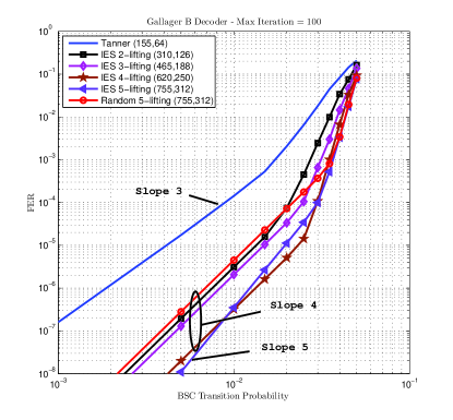
Figure 2: Comparison of the FER performance of the Tanner code and its liftings over the BSC (Example 3).

Example 4

In this example, we consider a regular $(504,252)$ code from [12] decoded by Gallager B algorithm. The dominant trapping sets in this case have critical number 3 and include $(3,3),(4,2)$, and $(5,3)$ trapping sets among others. The IES algorithm is used to design cyclic $N$-liftings of this code for $N=2$ to 6. The FER results of the liftings and the base code are reported in Fig. 3. Again, the performance of the $2$-lifting is similar to that of the code designed in [10]. All $(3,3)$ trapping sets are eliminated in the 2-lifting, but the survival of other trapping sets with critical number 3 keeps the minimal critical number at 3, and thus no change of FER slope compared to the base code is attained. Increasing $N$ to 3, however, eliminates all the trapping sets with critical number 3 and changes the slope of the FER to 4. The dominant trapping sets in this case are $(4,4)$ sets. Further increase of $N$ to 4 and 5 only reduces the number of $(4,4)$ trapping sets and thus results in a downward shift of the FER curve. For $N=6$, the algorithm can eliminate all the $(4,4)$ trapping sets, and thus increases the slope of the FER curve to 5. The dominant trapping sets in this case are $(5,5)$ sets.

For comparison, in Fig. 3, we have also shown the performance of a random 6-lifting of the $(504,252)$ code. As can be seen the performance of this code in the error floor region is far poorer than that of the designed $6$-lifting. In particular, the slope of the FER curve for this code is only 3 versus 5 for the designed code.

In this example, the parity-check matrix of the base code is full-rank, and all the liftings have the same rate of 0.5 as the base code.

Noteworthy is that while the 2-lifting has the same girth of $g=6$ as the base code, the girth for $N$-liftings, $N$ = 3 to 6, is increased respectively to 8, 8, 8 and 10.

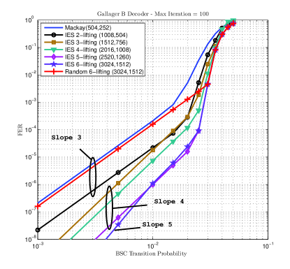
Figure 3: Comparison of the FER performance of the regular $(504,252)$ code and its liftings over the BSC (Example 4).

Example 5

In this example, we consider a randomly constructed rate-1/2 irregular $(200,100)$ code as the base code. The degree distributions for this code, optimized for Gallager A algorithm over the BSC [1], are $\lambda(x)=0.1115x^{2}+0.8885x^{3}$ and $\rho(x)=0.26x^{6}+0.74x^{7}$. The code has $g=6$. This code has a wide variety of dominant trapping sets under Gallager A algorithm, all with critical number 3.

We apply the IES algorithm to this code to design a cyclic $13$-lifting of length $2600$, rate 0.5 and $g=6$. The FER curves of the lifted code and the base code are presented in Fig. 4. As can be seen, the lifted code has a much better error floor performance compared to the base code. In fact, the minimum critical number for the lifted code is 5 versus 3 for the base code. For comparison, a rate-1/2 code of block length $2600$ with the same degree distribution and $g=6$ is constructed. The performance of this code is also given in Fig. 4. Clearly the performance of the lifted code is significantly better in the error floor region. In particular, the slope of the FER curve for the random code is the same as the base code and much less than that of the lifted code.

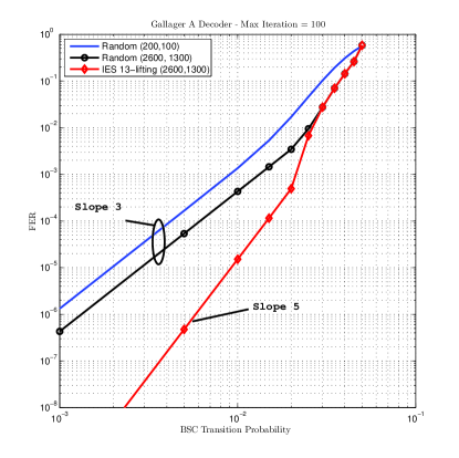
Figure 4: FER curves of the irregular $(200,100)$ code, its IES cyclic 13-lifting and a random irregular $(2600,1300)$ code with the same degree distribution over the BSC (Example 5).

Example 6

It is known that codes designed for a certain channel/decoding algorithm would also perform well for other channel/decoding algorithms [7]. In this example, we show that cyclically lifted codes designed for Gallager B algorithm in Examples 3 and 4 also perform very well on the binary-input AWGN channel under min-sum algorithm. The FER results for the 5-lifting of the Tanner code and the 6-lifting of the MacKay code are reported in Figures 5 and 6, respectively. In each figure, the performance of the corresponding base code and a similar random code (same block length and degree distributions) is also presented. One can see that at high SNR values, the designed codes perform far superior to the corresponding base codes and random codes. In particular, they show no sign of error floor for FER values down to about $10^{-8}$, and their FER decreases at a much faster rate compared to the base codes and random codes.

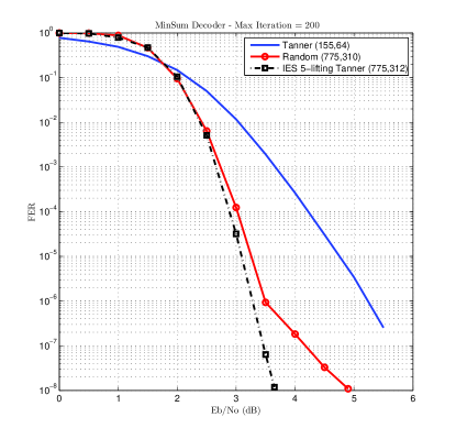
Figure 5: FER performance of the Tanner code, its IES cyclic 5-lifting and a random $(775,310)$ code with the same degree distribution over the BIAWGN channel (Example 6).

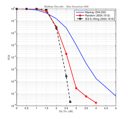
Figure 6: FER performance of the regular $(504,252)$ code, its IES cyclic 6-lifting and a random $(3024,1512)$ code with the same degree distribution over the BIAWGN channel (Example 6).

V CONCLUSIONS

In this work, cyclic liftings are proposed to improve the error floor performance of LDPC codes. The liftings are designed to eliminate the dominant trapping sets of the code by eliminating their constituent short cycles. The design approach is universal in that it can be applied to any decoding algorithm over any channel, as long as the dominant trapping sets are known and available. In addition, the liftings have the same degree distribution as the base code and are implementation friendly due to their cyclic structure. For base codes with full-rank parity-check matrices, the liftings also have the same rate as the base code and the performance improvement is achieved at the expense of larger block length. Compared to random codes or random liftings with the same block length and degree distribution, the designed codes perform significantly better in the error floor region.

While the cyclic liftings in this work were designed for Gallager A/B algorithms over the BSC, they also performed very well over the BIAWGN channel. In particular, the designed codes substantially outperformed similar random codes in the high SNR region.

References

- [1] L. Bazzi, T. J. Richardson and R. L. Urbanke, “Exact threshold and optimal codes for the binary-symmetric channel and Gallager s decoding algorithm A," IEEE Trans. Inform. Theory, vol. 50, pp. 2010 - 2021, Sept. 2004.
- [2] S. K. Chilappagari, M. Chertkov, M. G. Stepanov, and B. Vasic, “Instanton-based techniques for analysing and reduction of error floors of LDPC codes,“ IEEE Journ. Select. Areas Comm., vol. 27, no. 6, pp. 855-865, Aug. 2009.
- [3] S. K. Chilappagari, S. Sankaranarayanan, and B. Vasic, “Error floors of LDPC codes on the binary symmetric channel,” Proc. Int. Conf. Commun. (ICC 2006), Istanbul, Turkey, Jun. 2006, pp. 1089 - 1094.
- [4] C. A. Cole, S. G. Wilson, E. K. Hall, and T. R. Giallorenzi, “A general method for finding low error rates of LDPC codes," submitted to IEEE Trans. Inform. Theory, 2006.
- [5] C. Di, D. Proietti, I. E. Telatar, T. J. Richardson, and R. L. Urbanke, “Finite-length analysis of low-density parity-check codes on the binary erasure channel,” IEEE Trans. Inform. Theory, vol. 48, no.6, pp. 1570-1579, June 2002.
- [6] L. Dolecek, P. Lee, Z. Zhang, V. Anantharam, B. Nikolic and M. Wainwright, “Predicting error floors of structured LDPC codes: Deterministic bounds and estimates," IEEE Journ. Select. Areas Comm., vol. 27, no. 6, pp. 908 - 917, Aug. 2009.
- [7] M. Franceschini, G. Ferrari, and R. Raheli, “Does the performance of LDPC codes depend on the channel?,” IEEE Trans. Commun., vol. 54, no. 12, pp. 2129-2132, Dec. 2006.
- [8] R. G. Gallager, Low Density Parity Check Codes, Cambridge, MA: MIT Press, 1963.
- [9] Y. Han and W. E. Ryan, “Low-floor decoders for LDPC codes," IEEE Trans. Comm., vol. 57, no. 6, pp. 1663 - 1673, June 2009.
- [10] M. Ivkovic , S. K. Chilappagari, and B. Vasic, “Eliminating trapping sets in low-density parity-check codes by using Tanner graph covers,” IEEE Trans. Inform. Theory, vol. 54, no. 8, pp. 3763-3768, Aug. 2008.
- [11] X. Jiao, J. Mu, J. Song and L. Zhou, “Eliminating small stopping sets in irregular low-density parity-check codes," IEEE Comm. Lett., vol. 13, no. 6, pp. 435 - 437, June 2009.
- [12] D. J. C. Mackay, Encyclopedia of Sparse Graph Codes [Online]. Available: http://www.interference.phy.cam.ac.uk/mackay/codes/data.html.
- [13] T. Richardson, “Error floors of LDPC codes,” Proc. 41st Annual Allerton Conf. Commun., Control and Computing, Monticello, IL, Oct. 2003, pp. 1426 - 1435.
- [14] T. Richardson and R. Urbanke, “The capacity of low-density parity-check codes under message-passing decoding," IEEE Trans. Inform. Theory, vol. 47, no. 2, pp. 599 - 618, Feb. 2001.
- [15] T. Richardson and R. Urbanke, Modern Coding Theory, Cambridge University Press, 2008.
- [16] M. Stepanov and M. Chertkov, “Instanton analysis of low-density parity-check codes in the error floor regime,” Proc. IEEE Int. Symp. Inf. Theory (ISIT), Seattle, WA, July 2006, pp. 9 - 14.
- [17] R. M. Tanner, “A recursive approach to low complexity codes," IEEE Trans. Inform. Theory, vol. 27, pp. 533 - 547, Sept. 1981.
- [18] R. M. Tanner, D Sridhara, and T. Fuja, “A class of group-structured LDPC codes,” Proc. ISCTA 2001, Ambleside, England, 2001. [Online]. Available: http://www.soe.ucsc.edu/ tanner/isctaGrpStrLDPC.pdf.
- [19] D. Vukobratovic and V. Senk, “Evaluation and design of irregular LDPC codes using ACE spectrum," IEEE Trans. Comm., vol. 57, no. 8, pp. 2272 - 2278, Aug. 2009.
- [20] C.-C. Wang, “Code annealing and suppressing effect of the cyclically lifted LDPC code ensembles,” IEEE Information Theory workshop 2006, Chengdu, China, Oct. 2006, pp. 86 - 90.
- [21] C. Wang, S. R. Kulkarni, and V. Poor, “Finding all small error-prone substructures in LDPC codes,” IEEE Trans. Inform. Theory, vol. 55, no. 5, pp. 1976-1999, May 2009.
- [22] H. Xiao and A. H. Banihashemi, “Estimation of bit and frame error rates of finite-length low-density parity-check codes on binary symmetric channels,” IEEE Trans. Commun., vol. 55, no. 12, pp. 2234-2239, Dec. 2007.
- [23] H. Xiao and A. H. Banihashemi, “Error rate estimation of finite-length low-density parity-check codes decoded by soft-decision iterative algorithms," in Proc. 2008 IEEE ISIT, July 2008, pp. 439 - 443.
- [24] H. Xiao and A. H. Banihashemi, “Error rate estimation of low-density parity-check codes on binary symmetric channels using cycle enumeration,” IEEE Trans. Commun., vol 57, no. 6, pp. 1550-1555, June 2009.