IPPP/10/12 DCPT/10/24 IC/HEP/010-1

Constraining new physics with $B\rightarrow K^{*}\mu^{+}\mu^{-}$
in the early LHC era
Aoife Bharucha^,1 and William Reece^,2
1 IPPP, Department of Physics, University of Durham, Durham DH1 3LE, UK

² Blackett Lab, Physics Department, Prince Consort Road, London SW7 2AZ, UK

Abstract
We investigate the observables available in the angular distribution of $B\rightarrow K^{*}\mu^{+}\mu^{-}$ to identify those suitable for measurements in the first few years of LHC data taking. As experimental uncertainties will dominate, we focus on observables that are simple to measure, while maximizing the potential for discovery. There are three observables that may be extracted by counting signal events as a function of one or two decay angles and correspond to large features of the full angular distribution in the Standard Model: $A_{\mathrm{FB}}$, $F_{\mathrm{L}}$, and $S_{5}$. Two of these are well known in the experimental community; however, we show that measuring $S_{5}$ adds complementary sensitivity to physics beyond the Standard model. Like $A_{\mathrm{FB}}$, it features a zero–crossing point with reduced hadronic uncertainties at leading order and in the large recoil limit. We explore the experimental sensitivity to this point at LHCb and show that it may be measured with high precision due to the steepness of the $S_{5}$ distribution. Current experimental model independent constraints on parameter space are presented and predictions made for the values of the $A_{\mathrm{FB}}$ and $S_{5}$ zero–crossing points. The relative impact of LHCb measurements of $A_{\mathrm{FB}}$, $F_{\mathrm{L}}$, and $S_{5}$, with 2$\mbox{\,fb}^{-1}$ of integrated luminosity, is assessed. These issues are explored with a new model of the decay that can be used with standard simulation tools such as EvtGen.

Keywords : $B$-Physics; Beyond Standard Model; Rare Decays.

1 Introduction

The decay $\kern 1.79993pt\overline{\kern-1.79993ptB}{}_{d}\rightarrow\kern 1.99997pt\overline{\kern-1.99997ptK}{}^{*0}\mu^{+}\mu^{-}$ is a golden channel for the study of flavour changing neutral currents (FCNC) at the Large Hadron Collider (LHC). The four-body final state, as $\kern 1.99997pt\overline{\kern-1.99997ptK}{}^{*0}\rightarrow K\pi$, means that there is a wealth of information in the full-angular distribution that is complementary to that available in the widely studied $b\rightarrow s\gamma$ decays. In the presence of physics beyond the Standard Model (SM), new heavy degrees of freedom may enter the $b\rightarrow s$ loops. These can alter the decay amplitudes, affecting the full-angular distribution observed. This makes $\kern 1.79993pt\overline{\kern-1.79993ptB}{}_{d}\rightarrow\kern 1.99997pt\overline{\kern-1.99997ptK}{}^{*0}\mu^{+}\mu^{-}$ one of the most promising places in the flavour sector to search for new physics (NP) at the LHC (see Ref. [1] for a review). We concentrate on the large-recoil regime, where the energy of the $K^{*}$ is large such that QCD factorization is applicable. The low-recoil regime was described in Ref. [2], however at present form factors in this regime are not well known. A number of interesting measurements have already been made [3, 4, 5, 6, 7, 8, 9]. They are broadly in agreement with SM predictions; however, experimental precision is currently too low for firm conclusions to be drawn.

The properties of the full-angular distribution have been studied by many authors and a number of potential measurements have been identified; e.g. Refs [10, 11, 12, 13, 14, 15, 16]. Particular emphasis has been placed on finding angular observables with reduced theoretical uncertainties or enhanced sensitivity to particular classes of NP. However, in the first few years of LHC data taking the dominant sources of uncertainty will be experimental; thus, the emphasis should be on finding quantities that can be cleanly measured with relatively small uncertainties. Once very large data sets have been collected, it will be possible to use a full-angular analysis to extract the various underlying amplitudes directly [13, 17]. This will allow the determination of many theoretically clean observables. However, performing this kind of analysis will not be possible until detectors are very well understood and the number of collected signal events are in the thousands. Prior to this, symmetries and asymmetries of the full-angular distribution can be used to extract some observables individually from angular projections [18, 19, 20, 15, 14].

In this paper, we focus on observables that correspond to large features in the $\kern 1.79993pt\overline{\kern-1.79993ptB}{}_{d}\rightarrow\kern 1.99997pt\overline{\kern-1.99997ptK}{}^{*0}\mu^{+}\mu^{-}$ full-angular distribution and can be measured by counting the number of signal events as a function of one or two decay angles. We then investigate the relative experimental sensitivities to these observables at LHCb [21] and their projected impact on the allowed parameter space after measurements with 2$\mbox{\,fb}^{-1}$ of integrated luminosity. The rest of the paper is structured as follows: In the next section we give a brief overview of the theoretical framework employed with details of the decay amplitude calculation; in Sec. 3, observables that will be relevant for analyses with the first few years of LHC data are discussed, and details of benchmark NP models provided. We also summarize the impact of existing experimental measurements on constraining the NP contribution to the Wilson coefficients. In Sec. 5, we analyse the possibility of detecting NP effects at LHCb using our chosen observables. In Sec. 6, the potential impact of these measurements on parameter space is assessed. Finally, in Sec. 7, a short summary is given.

2 Theoretical Details

2.1 Introduction

A decay model following Ref. [22] has become the standard tool for studies of $\kern 1.79993pt\overline{\kern-1.79993ptB}{}_{d}\rightarrow\kern 1.99997pt\overline{\kern-1.99997ptK}{}^{*0}\mu^{+}\mu^{-}$ within the experimental community due to its inclusion in the decay simulator EvtGen [23]. A significantly improved version of that model with much greater support for the simulation of NP as well as a state-of-the-art SM treatment has been developed as part of the present work [24]. We present our theoretical framework in a way that allows direct comparison with Ref. [22], by expressing the decay amplitude in terms of the auxiliary functions used in that reference. Calculation of these requires Wilson coefficients, form factors and quantum-chromodynamics factorization (QCDF) corrections, as described in detail in this section.

2.2 Wilson Coefficients

$\,C_{1}(\mu)\quad$	$\,C_{2}(\mu)\quad$	$\,C_{3}(\mu)\quad$	$\,C_{4}(\mu)\quad$	$\,C_{5}(\mu)\quad$	$\,C_{6}(\mu)\quad$
-0.135	1.054	0.012	-0.033	0.009	-0.039

$\,C^{\mathrm{eff}}_{7}(\mu)$	$\,C^{\mathrm{eff}}_{8}(\mu)$	$\,\Delta C^{\mathrm{eff}}_{9}(\mu)$	$\,C^{\mathrm{eff}}_{10}(\mu)\,$
-0.306	-0.159	4.220	-4.093

Table 1: SM Wilson coefficients at $\mu=m_{b}=4.52{\mathrm{\,Ge\kern-1.00006ptV\!/}c^{2}}$, where $\Delta C^{\mathrm{eff}}_{9}(\mu)\sim C^{\mathrm{eff}}_{9}(\mu)-Y(q^{2})$.

The Wilson coefficients, $C_{i}(\mu)$, are process-independent coupling constants for the basis of effective vertices described by local operators, $\mathcal{O}_{i}(\mu)$, and encode contributions at scales above the renormalization scale, $\mu$. For a given NP model, new diagrams will become relevant and the $C_{i}(\mu)$’s may change from their SM values; additional operators may also become important. The weak effective Hamiltonian, neglecting doubly Cabibbo-suppressed contributions, ${\cal H}_{\rm{eff}}^{(u)}$, is given by

$${\cal H}_{\mathrm{eff}}=-\frac{4\,G_{F}}{\sqrt{2}}\lambda_{t}\left(C_{1}\mathcal{O}^{c}_{1}+C_{2}\mathcal{O}^{c}_{2}+\sum_{i=3}^{6}C_{i}\mathcal{O}_{i}+\sum_{j}(C_{j}\mathcal{O}_{j}+C_{j}^{\prime}\mathcal{O}^{\prime}_{j})\,\right),$$ (1)

where $j=7,8,9,10,P,S$, $G_{\mathrm{F}}$ is the Fermi constant, and $\lambda_{t}=V_{tb}V_{ts}^{*}$ is the relevant combination of Cabibbo–Kobayashi–Maskawa (CKM) matrix elements. The operators $\mathcal{O}$ and $\mathcal{O}^{\prime}$ are defined in Ref. [15], and a subset is given explicitly in App. A.

The primed operators have opposite chirality to the unprimed ones and their corresponding coefficients, $C_{i}^{\prime}(\mu)$, are suppressed by $m_{s}/m_{b}$ or vanish in the SM; however, they may be enhanced by NP. We neglect the contributions from $\mathcal{O}_{i}^{\prime}$ for $1\leq i\leq 6$ as they are either heavily constrained by experimental results or generically small; NP contributions to $\mathcal{O}^{\prime}_{7-10}$ may still be important and are included. We also include the scalar and pseudoscalar operators $\mathcal{O}^{(\prime)}_{S,P}$. These vanish in the SM but may arise in certain NP scenarios, for example in the case of an additional Higgs doublet.

The Wilson coefficients are calculated by matching the full and effective theories at the scale of the $W$ boson mass, $m_{W}$. For the SM Wilson coefficients, we aim at next-to-next-to-leading logarithmic (NNLL) accuracy. This requires calculating the matching conditions at $\mu=m_{W}$ to two-loop accuracy. This has been done in Ref. [26]. NP contributions are included to one-loop accuracy only, as two-loop corrections are expected to be small. This was shown explicitly for the MSSM in Ref. [27]. The Wilson coefficients must then be evolved down to the scale $\mu\sim m_{b}$. The evolution has been implemented using the full $10\times 10$ anomalous dimension matrix following Refs [28, 29, 30]. The primed operators, $\mathcal{O}^{\prime}_{7-10}$, are evolved as their unprimed equivalents; however, the scalar and pseudoscalar operators $\mathcal{O}^{(^{\prime})}_{S/P}$ are defined to be conserved currents and do not mix with the other operators and so do not require evolution. For convenience, we define the following combinations of Wilson coefficients:

$$C^{\mathrm{eff}}_{7} = \frac{4\pi}{\alpha_{s}}\,C_{7}-\frac{1}{3}\,C_{3}-\frac{4}{9}\,C_{4}-\frac{20}{3}\,C_{5}\,-\frac{80}{9}\,C_{6};$$

$$C^{\mathrm{eff}}_{8} = \frac{4\pi}{\alpha_{s}}\,C_{8}+C_{3}-\frac{1}{6}\,C_{4}+20C_{5}\,-\frac{10}{3}\,C_{6};$$

$$C^{\mathrm{eff}}_{9} = \frac{4\pi}{\alpha_{s}}\,C_{9}+Y(q^{2});$$

$$C^{\mathrm{eff}}_{10} = \frac{4\pi}{\alpha_{s}}\,C_{10};$$

$$C^{\prime\,\mathrm{eff}}_{7,8,9,10} = \frac{4\pi}{\alpha_{s}}\,C_{7,8,9,10}^{\prime}\,;$$ (2)

where $q^{2}$ is the invariant mass squared on the muon pair and $Y(q^{2})$ is defined in Ref. [31]. Tab. 1 gives the values of the Wilson coefficients at $\mu=m_{b,{\rm PS}}(2{\rm GeV})$ in the SM. The treatment of quark masses in the PS scheme is discussed in Sec. 2.6.

2.3 Form Factors

$\kern 1.79993pt\overline{\kern-1.79993ptB}{}_{d}\rightarrow\kern 1.99997pt\overline{\kern-1.99997ptK}{}^{*0}\mu^{+}\mu^{-}$ is characterized by eight form factors, $V(q^{2})$, $A_{0-3}(q^{2})$ and $T_{1-3}(q^{2})$. These are hadronic quantities that, for certain ranges in $q^{2}$, may be obtained by non-perturbative methods. Their definition in terms of hadronic matrix elements can be found, for example, in Ref. [32]. Lattice field theory currently offers a prediction for the form factor $T_{1}(0)$ relevant to $B\rightarrow K^{*}\gamma$ [33], but not for the others. However, QCD sum rules on the light cone (LCSR) is a well established alternative technique that provides results for the desired range in $q^{2}$ [32, 15]. It is an extension of classic QCD sum rules [34], in which matrix elements are evaluated via both operator product expansion and dispersive representation. Quark-hadron duality then leads to sum rules for the desired hadronic quantities. LCSR follows a similar procedure to obtain sum rules for the form factors, but the operator product expansion in terms of vacuum condenstates is replaced by a light-cone expansion in terms of universal light-cone meson distribution amplitudes. A comprehensive review of QCD sum rules and LSCR can be found in Ref. [35].

We use the full set of LCSR form factors in our model [32, 36], where the sum rules for all form factors except for $A_{0}$ were calculated at $\mathcal{O}(\alpha_{s})$ accuracy for twist-2 and-3 and tree-level accuracy for twist-4 contributions. Note that the normalization of the form factors we use differs slightly from Ref. [15], however this will not have much impact on the observables, as they are normalized by the total decay rate, so the effect will cancel out. We estimate the uncertainties using the values provided in Ref. [32] for $q^{2}=0$, as shown in Tab. 2. Note that $A_{3}(0)$ and $T_{2}(0)$ are not included in the table, as they can be found using the relations $A_{3}(0)=A_{0}(0)$ and $T_{2}(0)=T_{1}(0)$.

In the large energy limit of the $K^{*}$, the form factors satisfy certain relations and, therefore, can be reduced to two heavy-to-light or soft form factors, denoted $\xi_{\perp}$ and $\xi_{\parallel}$ [37, 38, 39, 40]. These reduced form factors are generally used within the QCDF framework [31, 41]. The relations are studied through appropriate ratios of the LCSR predictions for the full form factors in Appendix B of Ref. [15]. It is shown that those involving $\xi_{\perp}$ are almost independent of $q^{2}$, but those involving $\xi_{\parallel}$ have a definite dependence on $q^{2}$, so are probably more sensitive to the $1/m_{b}$ corrections neglected in QCDF.

	$F(0)$	$\Delta_{\rm tot}$	$\Delta_{a_{1}}$
$V$	0.411	0.033	0.44 $\delta_{a_{1}}$
$A_{0}$	0.374	0.034	0.39 $\delta_{a_{1}}$
$A_{1}$	0.292	0.028	0.33 $\delta_{a_{1}}$
$A_{2}$	0.259	0.027	0.31 $\delta_{a_{1}}$
$T_{1}$	0.333	0.028	0.34 $\delta_{a_{1}}$
$T_{3}$	0.202	0.018	0.18 $\delta_{a_{1}}$

Table 2: Form factors for $\kern 1.79993pt\overline{\kern-1.79993ptB}{}_{d}\rightarrow\kern 1.99997pt\overline{\kern-1.99997ptK}{}^{*0}\mu^{+}\mu^{-}$ from LCSR at $q^{2}=0$ [32], as described in Sec. 2.3. Here $\Delta_{\rm tot}$ is the total error arising from the uncertainty on all input parameters with the exception of the Gegenbauer moment $a_{1}$. $\Delta_{a_{1}}$ contains the uncertainty due to $a_{1}$, where $\delta_{a_{1}}$ is defined $\delta_{a_{1}}=a_{1}(K^{*},\,1\mathrm{GeV})-0.1$.

2.4 QCD Factorization Corrections

QCD factorization is a framework in which the $\mathcal{O}(\alpha_{s})$ corrections to $\kern 1.79993pt\overline{\kern-1.79993ptB}{}_{d}\rightarrow\kern 1.99997pt\overline{\kern-1.99997ptK}{}^{*0}\mu^{+}\mu^{-}$ can be calculated in the combined heavy-quark and large-recoil energy limit; this applies when the energy of the $K^{*}$ is large. These corrections take into account contributions that cannot be included in the form factors, such as the non-factorizable scattering effects arising from hard gluon exchange between the constituents of the $B$ meson.

Our calculation of the decay amplitude includes QCDF corrections at next-to-leading order (NLO) in $\alpha_{s}$ but leading order (LO) in $1/m_{b}$. These corrections are included in the definitions of $\mathcal{T}_{\parallel}(q^{2})$ and $\mathcal{T}_{\perp}(q^{2})$ found in Ref. [31] and are given in terms of $\xi_{\perp}$ and $\xi_{\parallel}$; however, $\mathcal{O}(\alpha_{s})$ factorizable corrections that arise from expressing the full form factors in terms of $\xi_{\perp}$ and $\xi_{\parallel}$ must then be subsumed. Following Ref. [15], we instead express our LO results for the decay amplitude in terms of the full form factors. Factorizable corrections are then redundant and the main source of $\mathcal{O}(1/m_{b})$ corrections is automatically included. In addition, we neglect weak annihilation corrections at LO in $1/m_{b}$ and $\mathcal{O}(\alpha_{s})$ as they are dependent on the numerically small Wilson coefficients $C_{3}$ and $C_{4}$.

We denote $\mathcal{T}^{\mathrm{NLO}}_{\parallel}(q^{2})$ and $\mathcal{T}^{\mathrm{NLO}}_{\perp}(q^{2})$ to be the analogues of $\mathcal{T}_{\parallel}(q^{2})$ and $\mathcal{T}_{\perp}(q^{2})$ from Ref. [31] with the only relevant $\mathcal{O}(\alpha_{s})$ contributions included. We also define $\mathcal{T}^{\prime\mathrm{NLO}}_{\parallel}(q^{2})$ and $\mathcal{T}^{\prime\mathrm{NLO}}_{\perp}(q^{2})$; the primes indicate that the unprimed Wilson coefficients should be replaced by their primed equivalents. In order to extend the results of Ref. [22] to include NLO corrections, we must make the following replacements:

$$C^{(\prime)\,\mathrm{eff}}_{7}T_{1}(q^{2})\quad\rightarrow \quad C^{(\prime)\,\mathrm{eff}}_{7}T_{1}(q^{2})+\mathcal{T}^{(\prime)\,\mathrm{NLO}}_{\perp}(q^{2});$$

$$C^{(\prime)\,\mathrm{eff}}_{7}T_{2}(q^{2})\quad\rightarrow \quad C^{(\prime)\,\mathrm{eff}}_{7}T_{2}(q^{2})+2\frac{E_{K^{*}}(q^{2})}{m_{B}}\mathcal{T}^{(\prime)\,\mathrm{NLO}}_{\perp}(q^{2});$$

$$C^{(\prime)\,\mathrm{eff}}_{7}T_{3}(q^{2})\quad\rightarrow \quad C^{(\prime)\,\mathrm{eff}}_{7}T_{3}(q^{2})+\mathcal{T}^{(\prime)\,\mathrm{NLO}}_{\perp}(q^{2})+\mathcal{T}^{(\prime)\,\mathrm{NLO}}_{\parallel}(q^{2});$$ (3)

where $E_{K^{*}}(q^{2})$ is the energy of the $K^{*}$ and $m_{B}$ is the mass of the B meson.

We have now introduced the Wilson coefficients, form factors and defined the QCD factorization corrections. These are all ingredients for the auxiliary functions describing the decay amplitude, as seen in the following subsection.

2.5 Decay Amplitude

The Hamiltonian defined in Eq. (1), combined with the standard definitions of the form factors, leads to the following decay amplitude [22, 42]:

$$\mathcal{M} \propto\left[\mathcal{T}_{\mu}^{1}\left(\bar{\mu}\,\gamma^{\mu}\,\mu\right)+\mathcal{T}_{\mu}^{2}\left(\bar{\mu}\,\gamma^{\mu}\gamma_{5}\,\mu\right)+\mathcal{S}(\bar{\mu}\,\mu)\right]$$ (4)

where

$$\mathcal{T}_{\mu}^{1} =A(q^{2})\epsilon_{\mu\rho\alpha\beta}\epsilon^{*\rho}\,\hat{p}^{\alpha}_{B}\,\hat{p}^{\beta}_{K^{*}}-iB(q^{2})\,\epsilon^{*}_{\mu}+iC(q^{2})(\epsilon^{*}\cdot\hat{p}_{B})\,\hat{p}_{\mu}+iD(q^{2})(\epsilon^{*}\cdot\hat{p}_{B})\,\hat{q}_{\mu}$$ (5)

$$\mathcal{T}_{\mu}^{2} =E(q^{2})\epsilon_{\mu\rho\alpha\beta}\,\epsilon^{*\rho}\hat{p}^{\alpha}_{B}\,\hat{p}^{\beta}_{K^{*}}-iF(q^{2})\,\epsilon^{*}_{\mu}+iG(q^{2})(\epsilon^{*}\cdot\hat{p}_{B})\,\hat{p}_{\mu}+iH(q^{2})(\epsilon^{*}\cdot\hat{p}_{B})\,\hat{q}_{\mu}$$ (6)

and

$$\mathcal{S} =i2\hat{m}_{K^{*}}(\epsilon^{*}\cdot\hat{p}_{B})\,I(q^{2}).$$ (7)

Here, $p_{B,K^{*}}$ and $m_{B,K^{*}}$ are the four-momenta and masses of the respective particles in the $B$ meson rest frame, $p\equiv p_{B}+p_{K^{*}}$, $q\equiv p_{B}-p_{K^{*}}$, and $\epsilon^{*}_{\mu}$ is the $K^{*}$ polarization vector. The circumflex denotes division by $m_{B}$ (e.g. $\hat{m}_{K^{*}}\equiv m_{K^{*}}/m_{B}$). The auxiliary functions $A$-$I(q^{2})$ follow Ref. [22]; however, we have updated the previous expressions to include additional primed, scalar, and pseudoscalar operators, as well as QCDF correction via $\mathcal{T}^{(^{\prime})\rm NLO}_{\parallel}(q^{2})$ and $\mathcal{T}^{(^{\prime})\rm NLO}_{\perp}(q^{2})$ as outlined in Sec. 2.4. They are defined as:

$$A(q^{2})= \frac{2}{1+\hat{m}_{K^{*}}}(C^{\mathrm{eff}}_{9}+C^{\prime\,\mathrm{eff}}_{9})V(q^{2})+\frac{4\hat{m}_{b}}{\hat{q}^{2}}\bigg{(}(C^{\mathrm{eff}}_{7}+C^{\prime\,\mathrm{eff}}_{7})T_{1}(q^{2})$$

$$+{\mathcal{T}}^{\rm NLO}_{\perp}(q^{2})+{\mathcal{T}}^{\prime\,\rm NLO}_{\perp}(q^{2})\bigg{)};$$ (8a)

$$B(q^{2})= (1+\hat{m}_{K^{*}})\bigg{\{}(C^{\mathrm{eff}}_{9}-C^{\prime\,\mathrm{eff}}_{9})A_{1}(q^{2})+\frac{2\hat{m}_{b}}{\hat{q}^{2}}(1-\hat{m}_{K^{*}})\bigg{(}(C^{\mathrm{eff}}_{7}-C^{\prime\,\mathrm{eff}}_{7})T_{2}(q^{2})$$

$$+2\hat{E}_{K^{*}}(q^{2})({\mathcal{T}}^{\rm NLO}_{\perp}(q^{2})-{\mathcal{T}}^{\prime\,\rm NLO}_{\perp}(q^{2}))\bigg{)}\bigg{\}};$$ (8b)

$$C(q^{2})= \frac{1}{1-\hat{m}_{K^{*}}^{2}}\bigg{\{}(1-\hat{m}_{K^{*}})(C^{\mathrm{eff}}_{9}-C^{\prime\,\mathrm{eff}}_{9})A_{2}(q^{2})$$

$$+2\hat{m}_{b}\bigg{(}(C^{\mathrm{eff}}_{7}-C^{\prime\,\mathrm{eff}}_{7})(T_{3}(q^{2})+\frac{1-\hat{m}_{K^{*}}^{2}}{\hat{q}^{2}}T_{2}(q^{2}))$$

$$+(1+\frac{(1-\hat{m}_{K^{*}}^{2})\,2\hat{E}_{K^{*}}(q^{2})}{\hat{q}^{2}})({\mathcal{T}}^{\rm NLO}_{\perp}(q^{2})-{\mathcal{T}}^{\prime\,\rm NLO}_{\perp}(q^{2}))$$

$$+{\mathcal{T}}^{\rm{NLO}}_{\parallel}(q^{2})-{\mathcal{T}}^{\prime\,\rm NLO}_{\parallel}(q^{2})\bigg{)}\bigg{\}};$$ (8c)

$$E(q^{2})= \frac{2}{(1+\hat{m}_{K^{*}})}(C^{\mathrm{eff}}_{10}+C^{\prime\,\mathrm{eff}}_{10})V(q^{2});$$ (8d)

$$F(q^{2})= (1+\hat{m}_{K^{*}})(C^{\mathrm{eff}}_{10}-C^{\prime\,\mathrm{eff}}_{10})A_{1}(q^{2});$$ (8e)

$$G(q^{2})= (C^{\mathrm{eff}}_{10}-C^{\prime\,\mathrm{eff}}_{10})\frac{A_{2}(q^{2})}{(1+\hat{m}_{K^{*}})};$$ (8f)

$$H(q^{2})= \frac{1}{\hat{q}^{2}}(C^{\mathrm{eff}}_{10}-C^{\prime\,\mathrm{eff}}_{10})\bigg{(}(1+\hat{m}_{K^{*}})A_{1}(q^{2})-(1-\hat{m}_{K^{*}})A_{2}(q^{2})$$

$$-2\hat{m}_{K^{*}}A_{0}(q^{2})\bigg{)}-\frac{\hat{m}_{K^{*}}m_{B}}{2\hat{m}_{\mu}}A_{0}(q^{2})(C_{P}-C_{P}^{\prime});$$ (8g)

$$I(q^{2})= -A_{0}(q^{2})(C_{S}-C_{S}^{\prime}).$$ (8h)

The recoil energy of the $K^{*}$ is given by

$$E_{K^{*}}(q^{2})=\frac{m_{B}^{2}+m_{K^{*}}^{2}-q^{2}}{2m_{B}}.$$ (9)

Using the equations of motion for the muons,

$$q^{\mu}(\bar{\mu}\gamma_{\mu}\,\mu)=0\qquad{\rm and}\qquad q^{\mu}(\bar{\mu}\gamma_{\mu}\gamma_{5}\,\mu)=-2m_{\mu}\bar{\mu}\gamma_{5}\,\mu,$$ (10)

where $m_{\mu}$ is the muon mass, we see that $D(q^{2})$ vanishes and $H(q^{2})$ is suppressed by a power of $m_{\mu}$. However, $H(q^{2})$ receives a pseudoscalar contribution inversely proportional to $m_{\mu}$ allowing for some sensitivity to $C_{P}-C_{P}^{\prime}$ [42]. The observables described in Sec. 3.1 (e.g. Eqs (16)–(17)) may be calculated directly from the amplitudes given in Eq. (8); the necessary formulae are presented in App. B and implemented in our model.

Parameter	Value	Ref.
$m_{s}$	0.104	[43]
$m_{c,{\rm PS}}(0.7{\rm\,GeV})$	1.5 GeV	[44]
$m_{b,{\rm PS}}(2{\rm\,GeV})$	4.52 GeV	[45]
$\hat{m}_{t}(\hat{m}_{t})$	162.3 GeV	[46]

Table 3: Quark masses

2.6 Numerical Input

2.6.1 Quark Masses

The calculation of the auxiliary functions requires the bottom quark pole mass, which is known to contain large long-distance corrections. To avoid this, a renormalization scheme, known as the potential subtraction scheme (PS), was introduced in Ref. [47]. The quark mass defined in the PS scheme has the advantage that the large infrared contributions are absent, while being numerically close to the pole mass. It is suitable for calculations in which the quark is nearly on-shell. Following Ref. [31], we replace the pole mass by the PS mass, $m_{\mathrm{PS}}(\mu_{f})$, using

$$m=m_{\mathrm{PS}}(\mu_{f})+\frac{4\alpha_{s}}{3\pi}\mu_{f}+\mathcal{O}(\alpha_{s}^{2})$$ (11)

and neglect any resulting terms of $\mathcal{O}(\alpha_{s}^{2})$. Here $\mu_{f}$ is the scale at which the PS mass is calculated. All occurrences of the symbol $m_{b}$ in our formulae refer to the PS mass, $m_{b,{\rm PS}}(2{\rm\,GeV})$, as shown in Tab. 3.

The operator $\mathcal{O}_{7}$ is defined in terms of the modified minimal subtraction ($\mathrm{\overline{MS}}$) mass. In the $\mathrm{\overline{MS}}$ scheme, the $1/\epsilon$ poles are simply removed, along with the associated terms in $\gamma$ and $4\pi$. Therefore, when the $b$ quark mass arises in combination with $C^{\mathrm{eff}}_{7}$, we replace the $\mathrm{\overline{MS}}$ mass, $\bar{m}$, by the pole mass, using

$$\bar{m}(\mu)=m\left(1+\frac{\alpha_{s}}{3\pi}\left(3\ln\frac{m_{b}^{2}}{\mu^{2}}-4\right)+\mathcal{O}(\alpha_{s}^{2})\right).$$ (12)

This leads to factorizable $\mathcal{O}(\alpha_{s})$ corrections to $\mathcal{T}^{\rm{NLO}}_{\perp/\parallel}(q^{2})$ and $\mathcal{T}^{\prime\rm{NLO}}_{\perp/\parallel}(q^{2})$ as found in Ref. [31].

For consistency, we calculate the charm quark pole mass using Eq. (11). Here the PS mass is taken from the most recent calculation as in Tab. 3. The resulting pole mass agrees with results in Ref. [43], where it is calculated from the $\overline{\rm{MS}}$ mass. The top quark mass enters the calculation of the Wilson coefficients, and for this we use the $\overline{\rm{MS}}$ mass in Tab. 3, as in Ref. [15].

Parameter	Value	Ref.	Parameter	Value	Ref.
$f_{B}$	$200\pm 25$ MeV	[48]	$a_{1,K^{*}}^{\perp}$(2 GeV)	$0.03\pm 0.03$	[49]
$\lambda_{B}$(2.2 GeV)	$0.51\pm 0.12$ GeV	[50]	$a_{1,K^{*}}^{\parallel}$(2 GeV)	$0.02\pm 0.02$	[49]
$f_{K^{*}}^{\perp}$(2 GeV)	$163\pm 8$ MeV	[49]	$a_{2,K^{*}}^{\perp}$(2 GeV)	$0.08\pm 0.06$	[49]
$\,f_{K^{*}}^{\parallel}\,$	$220\pm 5$ MeV	[49]	$\,a_{2,K^{*}}^{\parallel}\,$(2 GeV)	$0.08\pm 0.06$	[49]

Table 4: Hadronic parameters

2.6.2 Hadronic Parameters

In addition to the form factors described in Sec. 2.3, the QCDF corrections require light-cone distribution amplitudes and decay constants. The light-cone distribution amplitude for both the $B$ and $K^{*}$ mesons enter the hard scattering corrections. For the $B$ meson we follow the prescription in Ref. [31] using the values for $\mathchar 28931\relax_{B}$ given in Tab. 4. For the $K^{*}$ meson we use the standard Gegenabauer expansion,

$$\Phi_{K^{*}}^{m}=6u(1-u)(1+a_{1,K^{*}}^{m}C_{1}^{(3/2)}(2u-1)+a_{2,K^{*}}^{m}C_{2}^{(3/2)}(2u-1)),$$ (13)

for $m=\perp,\parallel$, taking the coefficients from Tab. 4. We also require the decay constants for both the $B$ and $K^{*}$ mesons. Additional parameters are summarized in Tab. 5.

3 Observables and New physics

Parameter	Value	Parameter	Value
$m_{B}$	5.28 GeV	$V_{\mathrm{us}}$	$0.226\pm 0.002$
$m_{K^{*}}$	0.896 GeV	$V_{\mathrm{ub}}$	$(3.93\pm 0.36)10^{-3}$
$m_{\mu}$	0.106 GeV	$\gamma$	$(77^{+30}_{-32})^{\circ}$
$M_{W}$	80.4 GeV	$G_{F}$	$(1.166)10^{-5}\,\mathrm{GeV}^{-2}$

Table 5: CKM matrix parameters, additional masses and constants from Ref. [43].

Having established the basic theoretical framework, we proceed to discuss experimental observables for $\kern 1.79993pt\overline{\kern-1.79993ptB}{}_{d}\rightarrow\kern 1.99997pt\overline{\kern-1.99997ptK}{}^{*0}\mu^{+}\mu^{-}$.

3.1 Observables

The full-angular decay distribution can be written as:

$$\frac{\rm{d}^{4}\Gamma}{\rm{d}q^{2}\,\rm{d}\cos\theta_{l}\,\rm{d}\cos\theta_{K^{*}}\,\rm{d}\phi}=\frac{9}{32\pi}I(q^{2},\theta_{l},\theta_{K^{*}},\phi),$$ (14)

where the angles $\theta_{K^{*}}$, $\theta_{l}$ and $\phi$ are defined as follows: $\theta_{K^{*}}$ is the angle between the $K^{-}$ and $\bar{B}$ in the rest frame of the $\kern 1.99997pt\overline{\kern-1.99997ptK}{}^{*}$, and is defined in the range $-1\leq\cos\theta_{K^{*}}\leq 1$; $\theta_{l}$ is defined as the angle between the $\mu^{-}$ and $\bar{B}$ in the di-muon centre of mass frame, and is defined in the range $-1\leq\cos\theta_{l}\leq 1$; $\phi$ is the angle between the normal to the $K$-$\pi$ plane and the normal to the di-muon plane, and is defined in the range $0\leq\phi\leq 2\pi$. For the conjugate decay, the angles are defined analogously, but with reference to the $K^{+}$ and $\mu^{+}$. We can then express $I(q^{2},\theta_{l},\theta_{K^{*}},\phi)$ in terms of these angles as follows:

$$I(q^{2},\theta_{l},\theta_{K^{*}},\phi) =I_{1}^{s}\sin^{2}\theta_{K^{*}}+I_{1}^{c}\cos^{2}\theta_{K^{*}}+(I_{2}^{s}\sin^{2}\theta_{K^{*}}+I_{2}^{c}\cos^{2}\theta_{K^{*}})\cos 2\theta_{l}$$

$$+I_{3}\sin^{2}\theta_{K^{*}}\sin^{2}\theta_{l}\cos 2\phi+I_{4}\sin 2\theta_{K^{*}}\sin 2\theta_{l}\cos\phi$$

$$+I_{5}\sin 2\theta_{K^{*}}\sin\theta_{l}\cos\phi$$

$$+(I_{6}^{s}\sin^{2}\theta_{K^{*}}+{I_{6}^{c}\cos^{2}\theta_{K^{*}}})\cos\theta_{l}+I_{7}\sin 2\theta_{K^{*}}\sin\theta_{l}\sin\phi$$

$$+I_{8}\sin 2\theta_{K^{*}}\sin 2\theta_{l}\sin\phi+I_{9}\sin^{2}\theta_{K^{*}}\sin^{2}\theta_{l}\sin 2\phi.$$ (15)

The angular coefficients $I_{i}^{(a)}$, where $i=1$ to $9$ and $a=s$ or $c$, describe the decay distribution. A natural set of observables was identified in Ref. [15] by taking combinations of these $I_{i}^{(a)}$’s that emphasize $C\!P$-conserving and $C\!P$-violating effects. These were defined as

$$S^{(s/c)}_{i} =(I^{(s/c)}_{i}+\bar{I}^{(s/c)}_{i})\Bigg{/}\frac{\rm{d}(\Gamma+\bar{\Gamma})}{\rm{d}q^{2}},$$ (16)

$$A^{(s/c)}_{i} =(I^{(s/c)}_{i}-\bar{I}^{(s/c)}_{i})\Bigg{/}\frac{\rm{d}(\Gamma+\bar{\Gamma})}{\rm{d}q^{2}},$$ (17)

where the $A^{(s/c)}_{i}$’s have also been studied in Ref. [14]. We introduce the rate average, which, for a variable $V(q^{2})$, is given by

$$\left<V\right>_{\text{1-6}\mathrm{\,Ge\kern-0.70004ptV}^{2}}=\int^{6\mathrm{\,Ge\kern-0.70004ptV}^{2}}_{1\mathrm{\,Ge\kern-0.70004ptV}^{2}}\mathrm{d}q^{2}\left(V(q^{2})\,\frac{\rm{d}(\Gamma+\bar{\Gamma})}{\rm{d}q^{2}}\right)\Bigg{/}\int^{6\mathrm{\,Ge\kern-0.70004ptV}^{2}}_{1\mathrm{\,Ge\kern-0.70004ptV}^{2}}\mathrm{d}q^{2}\frac{\rm{d}(\Gamma+\bar{\Gamma})}{\rm{d}q^{2}}.$$ (18)

Using Eq. (16), it is possible to reconstruct standard observables such as the forward-backward asymmetry, $A_{\mathrm{FB}}$, and the longtitudinal polarization fraction, $F_{\mathrm{L}}$:

$$A_{\mathrm{FB}}=\frac{3}{8}(2S_{6}^{s}+S_{6}^{c})\qquad\qquad\rm{and}\qquad\qquad F_{\mathrm{L}}=-S_{2}^{c}.$$ (19)

As explained in Sec. 1, our focus is on those observables that will be measurable at LHCb without a full-angular analysis. In order to keep the experimental complexity to a minimum, these observables should require information on only one or two of the angles. $A_{\mathrm{FB}}$, which depends only on $\theta_{l}$, and $F_{\mathrm{L}}$, which depends only on $\theta_{K^{*}}$, are well known examples. They can be expressed as:

$$A_{\mathrm{FB}}= \frac{4}{3}\left(\int_{0}^{1}-\int_{-1}^{0}\right)\rm{d}\theta_{l}\frac{\mathrm{d}^{2}(\Gamma+\bar{\Gamma})}{d\mathrm{q}^{2}\,\rm{d}\theta_{l}}\bigg{/}\frac{\mathrm{d}(\Gamma+\bar{\Gamma})}{\mathrm{d}q^{2}};$$ (20)

$$F_{\mathrm{L}}= \frac{1}{9}\left(16\int_{-1/2}^{1/2}\frac{\mathrm{d}(\Gamma+\bar{\Gamma})}{d\mathrm{q}^{2}\,\rm{d}\cos\theta_{K^{*}}}\bigg{/}\frac{\mathrm{d}(\Gamma+\bar{\Gamma})}{\mathrm{d}q^{2}}-11\right),$$ (21)

where the latter expression makes use of the massless lepton approximation. We also study the possibility of an early measurement of $$S_{5} \cos\theta_{K^{*}} \phi$$, which can be measured using only and . It is possible to express this as

$$S_{5}= \frac{4}{3}\left(\int_{0}^{\pi/2}+\int_{3\pi/2}^{2\pi}-\int_{\pi/2}^{3\pi/2}\right)\mathrm{d}\phi\left(\int_{0}^{1}-\int_{-1}^{0}\right)\rm{d}\cos\theta_{K^{*}}\frac{\mathrm{d}^{3}(\Gamma-\bar{\Gamma})}{\mathrm{d}q^{2}\,\rm{d}\cos\theta_{K^{*}}\,\rm{d}\phi}\bigg{/}\frac{\mathrm{d}(\Gamma+\bar{\Gamma})}{\mathrm{d}q^{2}}\,.$$ (22)

A comprehensive study of the effects of the Wilson coefficients on the above observables, and vice-versa, can be found in Ref. [15]. We note that $S_{3}$, $A_{7}$, and $A_{9}$ can also be extracted by the counting of signal events over one or two angles. $S_{3}$ is related to the well known and theoretically clean observable $A_{T}^{\left(2\right)}$ [12]; to be precise, $S_{3}$ equals $\frac{1}{2}(1-F_{\mathrm{L}})A_{T}^{\left(2\right)}$ in the massless lepton limit. While significant enhancement of $A_{T}^{\left(2\right)}$ is possible in the presence of non-SM $C^{\prime\,\mathrm{eff}}_{7}$ [51], the $\frac{1}{2}(1-F_{\mathrm{L}})$ prefactor implies that the enhancement is less pronounced in $S_{3}$ [20]. The smallness of $S_{3}$ means that the experimental sensitivity to $\left<S_{3}\right>_{\text{1-6}\mathrm{\,Ge\kern-0.70004ptV}^{2}}$ will be limited in the first few years of LHCb data taking; thus, the study of $S_{3}$ is thus left for other works [13]. Enhancements to $A_{7}$ and $A_{9}$ in the presence of NP phases can, however, be sizable [14] and could, in principle, lead to reasonable experimental resolutions, particularly for $\left<A_{9}\right>_{\text{1-6}\mathrm{\,Ge\kern-0.70004ptV}^{2}}$. However, these measurements will still be experimentally challenging in the first few years. For these reasons we choose to focus on $A_{\mathrm{FB}}$, $F_{\mathrm{L}}$ and $S_{5}$ for early study at LHCb.

As stated earlier, NP enters the calculations through contributions to the Wilson coefficients; constraints on these contributions are described in the Sec. 4. It is well known that for certain values of $q^{2}$, the observables $A_{\mathrm{FB}}$ and $S_{5}$ vanish. We refer to these values of $q^{2}$ as the zero-crossing points, $q_{0}^{2}(A_{\mathrm{FB}})$ and $q_{0}^{2}(S_{5})$. They are particularly sensitive to NP, and can be used to further constrain the values of the Wilson Coefficients. At leading order, in the large recoil limit, and for real values of the Wilson coefficients, it is possible to obtain simple expressions for $q_{0}^{2}(A_{\mathrm{FB}})$ [11, 31] and $q_{0}^{2}(S_{5})$:

$$q_{0}^{2}(A_{\mathrm{FB}})=-2m_{B}\,m_{b}\dfrac{C^{\mathrm{eff}}_{7}}{C^{\mathrm{eff}}_{9}};\qquad\qquad q_{0}^{2}(S_{5})=\dfrac{-m_{B}\,m_{b}(C^{\mathrm{eff}}_{7}+C^{\prime\,\mathrm{eff}}_{7})}{C^{\mathrm{eff}}_{9}+\hat{m}_{b}(C^{\mathrm{eff}}_{7}+C^{\prime\,\mathrm{eff}}_{7})}\,.$$ (23)

In deriving these results we make use of the soft form factors, following Refs [31, 41]. The two observables provide complementary sensitivity to NP through their differing dependence on the Wilson coefficients, and allow for sensitivity to both chiralities of $\mathcal{O}_{7}$. The cancellation of the soft form factors and the relative smallness of $\mathcal{O}(\alpha_{s})$ corrections mean that both zero–crossing points meet the criteria for theoretical cleanliness given in, e.g., Ref. [13]. In addition, we define the gradient of $A_{\mathrm{FB}}$ and $S_{5}$ at their zero-crossing points,

$$G_{0}(\mathcal{O})=\dfrac{\mathrm{d}\mathcal{O}}{\mathrm{d}q^{2}}\bigg{|}_{q_{0}^{2}(\mathcal{O})}\,,$$ (24)

where $\mathcal{O}$ is the observable $A_{\mathrm{FB}}$ or $S_{5}$ respectively. $A_{\mathrm{FB}}$ has also been studied in the context of $B\rightarrow K\pi l^{+}l^{-}$ [52], where expressions for $q_{0}^{2}(A_{\mathrm{FB}})$ and $G_{0}(A_{\mathrm{FB}})$ were determined for the case of an energetic kaon and soft pion. However, the kinematic region where the $K\pi$ pair is energetic is dominated by the $K^{*}$, and non-resonant effects can be neglected.

3.2 Overview of Specific Models and Effects on Wilson Coefficients

The observables for $\kern 1.79993pt\overline{\kern-1.79993ptB}{}_{d}\rightarrow\kern 1.99997pt\overline{\kern-1.99997ptK}{}^{*0}\mu^{+}\mu^{-}$ are most sensitive to the Wilson coefficients $C^{\mathrm{eff}}_{7}$, $C^{\mathrm{eff}}_{9}$, $C^{\mathrm{eff}}_{10}$ and their primed equivalents, so we concentrate on the NP contributions to these in this section. We also consider $C_{S}^{(\prime)}$ and $C_{P}^{(\prime)}$ for completeness; however, experimental sensitivity to their effects are expected to be limited in this decay.

• Flavour Blind MSSM (FBMSSM): Here the MFV version of the Minimal Supersymmetric Standard Model (MSSM) is modified by some flavour-conserving but $C\!P$-violating phases in the soft supersymmetry (SUSY) breaking trilinear couplings [53]. The Wilson coefficients we use correspond to those calculated in scenario FBMSSM II defined in Table 11 of Ref. [15]. The additional $C\!P$-violation contributes substantial complex phases to $C^{\mathrm{eff}}_{7}$, however there is no flavour structure beyond the SM, so primed operators are suppressed as in the SM. As in all SUSY models, scalar and pseudoscalar operators arise due to the additional Higgs doublet.

• General MSSM (GMSSM): Minimal flavour violation is not imposed, and generic flavour- and $C\!P$-violating soft SUSY-breaking terms are allowed [54]. The Wilson coefficients we use are close to the scenario GMSSM IV in Ref. [15], corresponding to large NP contributions to both $C^{\mathrm{eff}}_{7}$ and $C^{\prime\,\mathrm{eff}}_{7}$ allowed by existing experimental bounds (see Sec. 4).

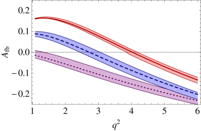
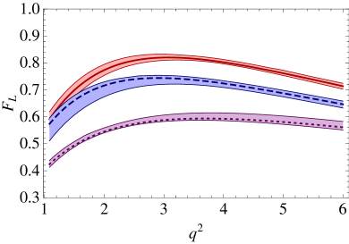
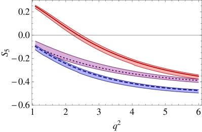
Figure 1: Theoretical predictions for $A_{\mathrm{FB}}$, $F_{L}$ and $S_{5}$. The red (continuous) line is the SM, the blue (dashed) line is the GMSSM, and the purple (dotted) line is the FBMSSM.

The Wilson coefficients in the above scenarios are given explicitly in Tab. 6. The central values for the distributions of $A_{\mathrm{FB}}$, $F_{\mathrm{L}}$, and $S_{5}$ are shown in Fig. 1 for the SM, the GMSSM, and FBMSSM, along with estimates of the theoretical uncertainties. The agreement with previous results is good. The predominant sources of the uncertainties are the form factors, hadronic parameters, and quark masses, which are determined as discussed in Sec. 2. We also include the uncertainty arising from varying the factorization scale, $\mu$, in the range $\mu\in[\mu/2,2\mu]$. The three distributions all show significant variation for the models considered here, as do the position or absence of the zero-crossing points in $A_{\mathrm{FB}}$ and $S_{5}$ in the range $q^{2}\in[1,6]\,\mathrm{GeV}^{2}$.

	Model
	SM	FBMSSM	GMSSM
$C^{\mathrm{eff}}_{7}(\mu)$	-0.306	-0.031+0.475i	-0.186+0.002i
$C^{\prime\,\mathrm{eff}}_{7}(\mu)$	-0.007	-0.008+0.003i	-0.155+0.160i
$C^{\mathrm{eff}}_{8}(\mu)$	-0.159	-0.085+0.149i	-0.062+0.004i
$C^{\mathrm{eff}}_{8}(\mu)$	-0.004	-0.000+0.001i	-0.330+0.336i
$\Delta C^{\mathrm{eff}}_{9}(\mu)$	4.220	-4.257+0.000i	-4.231+0.000i
$C^{\prime\,\mathrm{eff}}_{9}(\mu)$	0.000	-0.002+0.000i	-0.018+0.000i
$C^{\mathrm{eff}}_{10}(\mu)$	-4.093	-4.063+0.000i	-4.241+0.000i
$C^{\prime\,\mathrm{eff}}_{10}(\mu)$	0.000	-0.004+0.000i	-0.003+0.003i
$\hat{C}_{S}(\mu)/\mathrm{GeV}^{-1}$	0.000	-0.044-0.056i	-0.000+0.001i
$\hat{C}_{P}(\mu)/\mathrm{GeV}^{-1}$	0.000	-0.043+0.054i	-0.001+0.001i

Table 6: NP Wilson coefficients at $\mu=m_{b,\mathrm{PS}}(2{\mathrm{\,Ge\kern-1.00006ptV\!/}c^{2}})=4.52{\mathrm{\,Ge\kern-1.00006ptV\!/}c^{2}}$ in the FBMSSM and GMSSM as described in Sec. 3.2, where $\hat{C}_{X}(\mu)=(C_{X}-C_{X}^{\prime})(\mu)$ for $X=S$ or $P$.

4 Constraints

Experimental results can be used to constrain the NP contributions, denoted $C_{i}^{\mathrm{NP}}$, to the Wilson coefficients: we define $C_{i}=C_{i}^{\mathrm{SM}}+C_{i}^{\mathrm{NP}}$. We can then determine possible model-independent effects of NP on $\kern 1.79993pt\overline{\kern-1.79993ptB}{}_{d}\rightarrow\kern 1.99997pt\overline{\kern-1.99997ptK}{}^{*0}\mu^{+}\mu^{-}$. The most important constraints on the Wilson coefficients are from the following measurements:

• Branching Ratio for $B_{s}\rightarrow\mu^{+}\mu^{-}$: This is used to constrain the possible NP contribution to the scalar and pseudoscalar operators. To calculate the branching ratio we use the standard result from Ref. [15]

  $$\mathcal{B}(B_{s}\rightarrow\mu^{+}\mu^{-})=\tau_{B_{s}}f_{B_{s}}^{2}m_{B_{s}}\frac{\alpha_{EM}^{2}G_{F}^{2}}{16\pi^{3}}|V_{tb}V^{*}_{ts}|^{2}\sqrt{1-\frac{4m_{\mu}^{2}}{m_{B_{s}}^{2}}}(|S|^{2}\left(1-\frac{4m_{\mu}^{2}}{m_{B_{s}}^{2}}\right)+|P|^{2}),$$ (25)

  with the definitions

  $$S=\frac{m_{B_{s}}^{2}}{2}(C_{S}-C_{S}^{\prime});\qquad P=\frac{m_{B_{s}}^{2}}{2}(C_{P}-C_{P}^{\prime})+m_{\mu}(C^{\mathrm{eff}}_{10}-C^{\prime\,\mathrm{eff}}_{10}).$$ (26)

  We use $f_{B_{s}}=0.259\pm 0.032$ GeV [55], $\tau_{B_{s}}=1.456\pm 0.03$ps [56] and $m_{B_{s}}=5.37$ GeV [43], and other numerical parameters as in Ref. [15]. In agreement with existing results, we find the SM prediction, $\mathrm{BR}(B_{s}\rightarrow\mu^{+}\mu^{-})=(3.70\pm 0.31)\cdot 10^{-9}$, to be well below the current experimental upper bound $3.6\cdot 10^{-8}$ [57, *CDF:2009].

• Branching Ratio for $B\rightarrow X_{s}l^{+}l^{-}$: We compare NP predictions for $\mathcal{B}(B\rightarrow X_{s}l^{+}l^{-})_{\text{1-6}\,\mathrm{GeV}^{2}}$ to the mean experimental value $(1.60\pm 0.51)\cdot 10^{-6}$, as adopted in Ref. [14], combining the results of BABAR, $(1.8\pm 0.7\pm 0.5)\cdot 10^{-6}$ [59], and Belle, $(1.49_{-0.32}^{+0.41}\pm 0.50)\cdot 10^{-6}$ [60]. This helps to constrain the NP contribution to $C^{(\prime)\,\mathrm{eff}}_{7,9,10}$ as well as $C^{(^{\prime})}_{S,P}$. As an inclusive mode, the calculation for the region $q^{2}\in[1,6]\mathrm{\,Ge\kern-1.00006ptV}^{2}$ of the branching ratio is theoretically clean. We use the expression for the differential decay distribution in Ref. [61], but also include the NLO corrections computed in Ref. [62], and the contribution of the primed operators as in Ref. [63]. Using our parameters we find $\mathcal{B}(B\rightarrow X_{s}l^{+}l^{-})=(1.96\pm 0.11)\cdot 10^{-6}$ for the SM.

• Branching Ratio for $B\rightarrow X_{s}\gamma$: The current experimental average for $\mathrm{E}_{\gamma}>1.6\,\mathrm{GeV}$ is $\,\mathcal{B}(B\rightarrow X_{s}\gamma)=(3.52\pm 0.23\pm 0.09)\cdot 10^{-4}$, as calculated by the Heavy Flavor Averaging Group [56]. We use the recent theoretical SM result of Ref. [64], $(3.28\pm 0.25)\cdot 10^{-4}$ for $\mathrm{E}_{\gamma}>1.6\,\mathrm{GeV}$, and include NP effects as in Ref. [51]. The SM calculation makes use of the kinetic renormalization scheme for determining $m_{c}$ and $m_{b}$; an alternative calculation using the 1S scheme leads to a branching ratio of $(3.15\pm 0.23)\cdot 10^{-4}$ [65, 66]; however, our results are not sensitive to the difference between these two values.

• Time dependent $C\!P$ Asymmetry $S(B\rightarrow K^{*}\gamma$): This constraint is sensitive to the photon polarization, and, hence, to $C^{\prime\,\mathrm{eff}}_{7}$. This should be compared to $S(B\rightarrow K^{*}\gamma)=(-1.6\pm 2.2)\cdot 10^{-1}$ from experiment [56]. Our SM result $S(B\rightarrow K^{*}\gamma)=(-0.26\pm 0.05)\cdot 10^{-1}$ agrees with that of Ref. [14] within uncertainties. In Refs [67, 68], the soft gluon contribution was calculated, leading to a small correction to the predicted value. This is neglected in our treatment as it has little effect on the constraining power of the experimental measurement.

• Integrated Forward-Backward Asymmetry $\langle A_{\mathrm{FB}}\rangle_{\text{1-6}\,\mathrm{GeV}^{2}}$ for $\kern 1.79993pt\overline{\kern-1.79993ptB}{}_{d}\rightarrow\kern 1.99997pt\overline{\kern-1.99997ptK}{}^{*0}\mu^{+}\mu^{-}$: We use the existing $\kern 1.79993pt\overline{\kern-1.79993ptB}{}_{d}\rightarrow\kern 1.99997pt\overline{\kern-1.99997ptK}{}^{*0}\mu^{+}\mu^{-}$ measurements as constraints. Recently Belle has made a measurement of the forward-backward asymmetry, and finds the integrated $A_{\mathrm{FB}}$ value in the region 1-6$\,\mathrm{GeV}^{2}$ to be $-0.26\pm 0.29$ [8]. This is to be compared to our SM prediction of $0.04\pm 0.03$, which is in agreement with the recent result in Ref. [69]. This observable constrains the Wilson coefficients as seen in Tab. 7. We look forward to a 1-6$\,\mathrm{GeV}^{2}$ measurement from CDF with great interest [9].

• Integrated Longitudinal Polarization Fraction $\langle F_{\mathrm{L}}\rangle_{\text{1-6}\,\mathrm{GeV}^{2}}$ for $\kern 1.79993pt\overline{\kern-1.79993ptB}{}_{d}\rightarrow\kern 1.99997pt\overline{\kern-1.99997ptK}{}^{*0}\mu^{+}\mu^{-}$: Belle has also recently measured the Longitudinal Polarization Fraction to be $0.67\pm 0.24$ [8]. This should be compared to our SM prediction $0.76\pm 0.08$, also in agreement with Ref. [69]. Again this constraint affects Wilson coefficients as seen in Tab. 7.

Observable	Wilson Coefficients
$A_{\mathrm{FB}}$	$C^{\mathrm{eff}}_{7}$, $C^{\mathrm{eff}}_{9}$
$F_{\mathrm{L}}$	$C^{\mathrm{eff}}_{7}$, $C^{\prime\,\mathrm{eff}}_{7}$,$C^{\mathrm{eff}}_{8}$,$C^{\prime\,\mathrm{eff}}_{9}$, $C^{\mathrm{eff}}_{10}$, $C^{\prime\,\mathrm{eff}}_{10}$
$S_{5}$	$C^{\mathrm{eff}}_{7}$, $C^{\prime\,\mathrm{eff}}_{7}$, $C^{\mathrm{eff}}_{9}$, $C^{\prime\,\mathrm{eff}}_{10}$

Table 7: Relevant observables and the Wilson coefficients they most strongly depend on [15].

Observable	Experiment	SM Theory
$\mathcal{B}(B_{s}\rightarrow\mu^{+}\mu^{-})$	$3.6\cdot 10^{-8}$ [57, *CDF:2009]	$(3.70\pm 0.31)\cdot 10^{-9}$
$\,\mathcal{B}(B\rightarrow X_{s}l^{+}l^{-})_{\text{1-6}\,\mathrm{GeV}^{2}}\,$	$(1.60\pm 0.51)\cdot 10^{-6}$ [14]	$(1.97\pm 0.11)\cdot 10^{-6}$
$\mathcal{B}(B\rightarrow X_{s}\gamma)$	$(3.52\pm 0.23\pm 0.09)\cdot 10^{-4}$ [56]	$(3.28\pm 0.25)\cdot 10^{-4}$
$S(B\rightarrow K^{*}\gamma)$	$(-1.6\pm 2.2)\cdot 10^{-1}$ [56]	$(-0.26\pm 0.05)\cdot 10^{-1}$
$\langle A_{\mathrm{FB}}\rangle_{\text{1-6}\,\mathrm{GeV}^{2}}$	$-0.26\pm 0.29$ [8]	$0.04\pm 0.03$
$\langle F_{L}\rangle_{\text{1-6}\,\mathrm{GeV}^{2}}$	$0.67\pm 0.24$ [8]	$0.76\pm 0.08$

Table 8: Experimental measurements used as constraints, along with theoretical predictions in the SM.

In order to assess the impact of these constraints on the NP contributions to the underlying Wilson coefficients in as general a way as possible, we have performed a semi-random walk through parameter space. We allow $(C_{S}-C_{S}^{\prime})$, $(C_{P}-C_{P}^{\prime})$ and the NP components of $C^{(\prime)\,\mathrm{eff}}_{7-10}$ to vary simultaneously, both in magnitude and phase. To our knowledge this has not been done in previous studies. At each randomly chosen point in parameter space, predictions are made for the six observables listed above. The point is then either accepted or rejected using a modified $\chi^{2}$ metric that treats experimental uncertainties as being normally distributed, but theoretical uncertainties as having uniform probability within the specified range. Following traditional minimization techniques, the random walk is guided by this modified $\chi^{2}$ so that regions with lower values may be identified. Using this method, a sample of $2.5\cdot 10^{5}$ independent sets of Wilson coefficients was produced. Each set results in predictions for the observables listed above with better than $2\sigma$ agreement with current measurements. It was found that the agreement between existing measurements and the SM is excellent, with a $\chi^{2}$ per degree of freedom of $0.35$. While this is not implausible for six degrees of freedom, the level of agreement suggests that more detailed study of the theoretical uncertainties will be required as experimental resolutions improve.

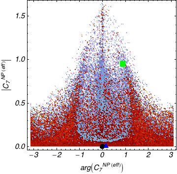
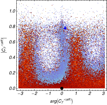
Figure 2: [Colour online] Allowed parameter space for the NP contribution to $C^{\mathrm{eff}}_{7}$ and $C^{\prime\,\mathrm{eff}}_{7}$ at the scale $\mu=m_{W}$, as described in Sec. 4. Points with a compatibility with data of 68% or better are drawn with a dark (red) colour palette, while those with less than this are drawn with a light (blue) palette. The SM point is shown in black at the origin, while the FBMSSM is a green square and the GMSSM is a blue triangle. The Wilson coefficients for these models are shown in Tab. 6.

Fig. 2 shows the range of values found for the phase and magnitude of the NP contribution to $C^{\mathrm{eff}}_{7}$ and $C^{\prime\,\mathrm{eff}}_{7}$ (at the scale $\mu=m_{W}$) during the parameter space exploration. The colour index shows the mean value of the probability that a point is compatible with current experimental results. Areas with probability greater than $1\sigma$ are shaded red, while those with less than $1\sigma$ are shaded blue. The outline of the $1\sigma$ contour can clearly be seen. The values of the Wilson coefficients for the SM, FBMSSM, and GMSSM are also shown.

Fig. 2 can be compared to Fig. 2 from Ref. [14], in which $C^{\mathrm{eff}}_{7}$ and $C^{\prime\,\mathrm{eff}}_{7}$ are assumed to be real and all other Wilson coefficients SM-like. The effects of weakening these assumptions can be seen. Similar figures are shown for the other Wilson coefficients in Figs 3 and 4. The allowed regions of parameter space are still large, particularly if NP phases are allowed. In contrast to Ref. [14], constraints from $A_{\mathrm{FB}}$ measurements at high–$q^{2}$ (low recoil) are not included as we feel that NLO effects are not under control in this region. The effect of this constraint may be seen by comparing our $C^{\mathrm{eff}}_{10}$ figure, shown in Fig. 4, with that in Fig. 2 of Ref. [14].

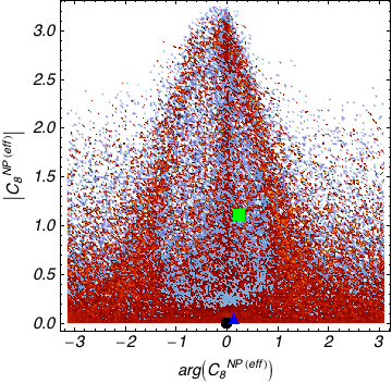
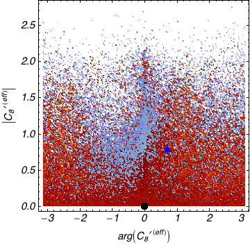
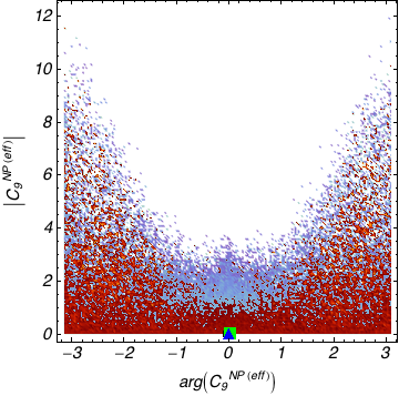
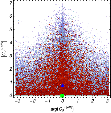
Figure 3: [Colour online] Allowed parameter space for the Wilson coefficients $C^{(\prime)\,\mathrm{eff}}_{8-9}$ after applying relevant $b\rightarrow s$ experimental constraints. The colour coding is the same as in Fig. 2.

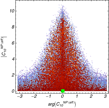
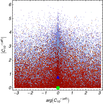
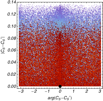
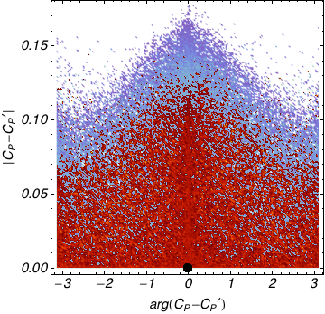
Figure 4: [Colour online] Allowed parameter space for the Wilson coefficients $C^{(\prime)\,\mathrm{eff}}_{10}$ and $(C_{S,P}-C_{S,P}^{\prime})$ after applying relevant $b\rightarrow s$ experimental constraints. The colour coding is the same as in Fig. 2.

The ensemble of constrained NP models can also be used to explore the likely values of the $A_{\mathrm{FB}}$ and $S_{5}$ zero-crossing points in the range $q^{2}\in[0.5,15]\mathrm{\,Ge\kern-1.00006ptV}^{2}$. While it should be noted that theoretical uncertainties are not well controlled over this $q^{2}$ range, the majority of points within the $1\sigma$ contour lie within the theoretically clean region, $q^{2}\in[1,6]\mathrm{\,Ge\kern-1.00006ptV}^{2}$ (see Fig. 5a). It was found that 8% of the parameter space points considered had no $A_{\mathrm{FB}}$ zero-crossing in the range $q^{2}\in[0.5,15]\mathrm{\,Ge\kern-1.00006ptV}^{2}$. For $S_{5}$, only 2% of points had no zero-crossing in the same range. Fig. 5b shows the $A_{\mathrm{FB}}$ and $S_{5}$ gradients at their zero-crossing points. We find that, for the majority of points, $G_{0}(S_{5})$ is greater than $G_{0}(A_{\mathrm{FB}})$. This will have an impact for the $q^{2}_{0}(S_{5})$ experimental analysis discussed in the Sec. 5.4.2.

To summarize, in this section we have considered six existing experimental constraints, and used these to determine the allowed regions in parameter space for the NP contribution to the Wilson coefficients. These allowed values for the Wilson coefficients were then used to find corresponding predictions for $q^{2}_{0}(S_{5})$, $q^{2}_{0}(A_{\mathrm{FB}})$, $G_{0}(S_{5})$, and $G_{0}(A_{\mathrm{FB}})$. In the following sections, we investigate the experimental sensitivity to the observables $A_{\mathrm{FB}}$, $S_{5}$, and $F_{\mathrm{L}}$, and how measurements of these could have an impact on the allowed NP contributions to the Wilson coefficients.

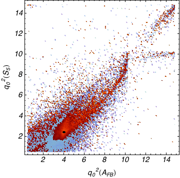
(a)

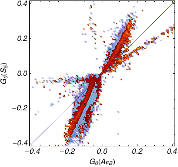
(b)

Figure 5: [Colour online] Fig. LABEL:sub@fig:constraints-zero shows allowed values of the $A_{\mathrm{FB}}$ and $S_{5}$ zero-crossing points in the range $q^{2}\in[0.5,15]\mathrm{\,Ge\kern-1.00006ptV}^{2}$. The SM point and its uncertainty is shown as a black ellipse. Fig. LABEL:sub@fig:constraints-grad shows the gradient of the $A_{\mathrm{FB}}$ and $S_{5}$ at the zero-point. For comparison, the line $G_{0}(S_{5})=G_{0}(A_{\mathrm{FB}})$ is included. In each case the colour index has the same meaning as in Fig. 2.

5 Experimental Sensitivities

Three observables that can be measured as a function of $q^{2}$ by counting signal events in specific angular bins, using Eqs (20)–(22), were highlighted in Sec. 3.1: $A_{\mathrm{FB}}$, $F_{\mathrm{L}}$, and $S_{5}$. These observables should be suitable for early measurement at LHCb. In the following, we estimate the experimental sensitivities in order to make a fair comparison between these observables.

LHCb is expected to collect $\sim 6.2\cdot 10^{3}$ signal events per 2$\mbox{\,fb}^{-1}$ of integrated luminosity with a signal to background ratio of approximately four [70, 71]. With relatively small data sets it should be possible to extract the values of these observables integrated over $q^{2}$. These measurements provide an early opportunity to discover NP in $b\rightarrow s$ transitions. For larger data sets it will be possible to map out the dependence on $q^{2}$ as well, allowing for additional NP discrimination. Studies of these two approaches can be found in Refs [18, 19] for the observable $A_{\mathrm{FB}}$.

To assess the impact of each potential measurement on the allowed NP parameter space, simple analyses have been developed to extract the $q^{2}$ integrated values of $A_{\mathrm{FB}}$, $F_{\mathrm{L}}$, and $S_{5}$ in the region $q^{2}\in[1,6]\mathrm{\,Ge\kern-1.00006ptV}^{2}$. In addition, analyses have been constructed to extract the $q^{2}$ dependence of $A_{\mathrm{FB}}$ and $S_{5}$, along with their zero-crossing points; the latter can be found numerically from the $A_{\mathrm{FB}}(q^{2})$ and $S_{5}(q^{2})$ distributions. In order to minimize the experimental uncertainties on these points, a larger region of $q^{2}\in[0.5,8.5]\mathrm{\,Ge\kern-1.00006ptV}^{2}$ was used for these analyses following Ref. [19]. An ensemble of 1200 simulated $\kern 1.79993pt\overline{\kern-1.79993ptB}{}_{d}\rightarrow\kern 1.99997pt\overline{\kern-1.99997ptK}{}^{*0}(\rightarrow K\pi)\mu^{+}\mu^{-}$ data sets was created, each containing the (Poisson fluctuated) number of signal and background expected from 2$\mbox{\,fb}^{-1}$ of integrated luminosity at LHCb. Other integrated luminosities were obtained by linearly scaling the yield estimates. Each analysis was then run in turn on the data sets in order to estimate the statistical uncertainty expected for each measurement. This allows for a fair comparison to be made between observables for a given integrated luminosity.

5.1 Data Set Generation

The theoretical framework introduced in Sec. 2 was implemented as a plug-in for the standard decay tree simulation tool EvtGen [23]. This allows $\kern 1.79993pt\overline{\kern-1.79993ptB}{}_{d}\rightarrow\kern 1.99997pt\overline{\kern-1.99997ptK}{}^{*0}(\rightarrow K\pi)\mu^{+}\mu^{-}$ events to be simulated. A simplified background sample was generated separately. This was flat in the three decay angles defined in Sec. 3.1 but followed the signal distribution in $q^{2}$ and a gently falling exponential in the $B$ invariant mass, $m_{B}$. All events had $m_{B}$ within a wide window ${}^{+250}_{-150}\mathrm{\,Me\kern-1.00006ptV}$ around the nominal $B$ mass. A central signal region was also defined with width $\pm 50\mathrm{\,Me\kern-1.00006ptV}$. Events outside of this region were assumed to be part of a background dominated side-band. Signal and background events were generated following the relative normalization given in Refs [70, 71]. For each event in a data set, the three decay angles, $q^{2}$ and $m_{B}$ were determined and used as input for each analysis.

5.2 $q^{2}$ Integrated Analyses

The integrated quantities can be extracted by estimating the number of signal events in each angular bin using a fit to the $m_{B}$ distribution. The signal contribution was parametrized as a Gaussian with an exponential tail, while the background was modelled as an exponential with a negative coefficient. A fit was performed to each data set to extract the signal and background shape parameters for that sample. Each sample was then reduced into the relevant angular bins. For $A_{\mathrm{FB}}$, following Eq. (20) these bins would be $\cos\theta_{l}\in[-1,0]$ and $\cos\theta_{l}\in[0,1]$ for all events in the range $q^{2}\in[1,6]\mathrm{\,Ge\kern-1.00006ptV}^{2}$. To extract an estimate of the number of signal and background events in each angular bin, a separate fit to the $m_{B}$ signal and background distributions was then performed, keeping all shape parameters fixed. The value of $\left<A_{\mathrm{FB}}\right>_{\text{1-6}\mathrm{\,Ge\kern-0.70004ptV}^{2}}$ was determined with Eq. (20). A similar procedure was applied to Eqs (21) and (22) to extract $\left<F_{\mathrm{L}}\right>_{\text{1-6}\mathrm{\,Ge\kern-0.70004ptV}^{2}}$ and $\left<S_{5}\right>_{\text{1-6}\mathrm{\,Ge\kern-0.70004ptV}^{2}}$.

5.3 $q^{2}$ Dependent Analyses

Following Ref. [19], a polynomial shape was fit to the $q^{2}$ distribution in each angular bin. The method proceeds as in Sec. 5.2, using the $B$ mass distribution to find the total number of signal and background events in each angular bin. However, the background shape extracted is used to estimate the number of signal events in the $B$ mass signal window. The $q^{2}$ dependence of the signal and background distributions was parametrized using second and third order Chebyshev polynomials respectively. A simultaneous fit in the signal and side-band regions of the $B$ mass distribution was used to determine the shape parameters of signal and background polynomials using the relative signal/background normalization found from the $B$ mass fits. In the case of $A_{\mathrm{FB}}$, the procedure would lead to the extraction of two $q^{2}$ dependent signal polynomials: one for events with $\cos\theta_{l}\in[-1,0]$ and the other for $\cos\theta_{l}\in[0,1]$. The value of $A_{\mathrm{FB}}$ ($q^{2}$) can then be found using these polynomials and Eq. (20). The $A_{\mathrm{FB}}$ zero-crossing point was found numerically from the combined functions. A similar approach was applied to $S_{5}$ and its zero-crossing; however, six angular bins in $\theta_{K^{*}}$ and $\phi$ were required.

5.4 Results

When comparing different observables and analyses it is useful to consider the mean expected experimental sensitivity for a given integrated luminosity. These expected sensitivities can be calculated from the ensemble of toy LHCb experiments introduced in Secs 5.2 and 5.3. 1200 individual experiments were performed, and for each one a value of, for example, $q^{2}_{0}(A_{\mathrm{FB}})$ was found. Following Ref. [13], the mean, one and two sigma contours could then be found from these results. The method used allows for non-normally distributed results by putting the ensemble in numerical order and then selecting the values closest to the contour. Any biases introduced can be identified by comparing the median result and input value. Example ensembles are shown in Fig. 7 for $q^{2}_{0}(A_{\mathrm{FB}})$ and $q^{2}_{0}(S_{5})$, assuming 2$\mbox{\,fb}^{-1}$ of LHCb data and following the SM.

5.4.1 Integrated Quantities

The estimated $1\sigma$ sensitivities for the integrated observables $\left<A_{\mathrm{FB}}\right>_{\text{1-6}\mathrm{\,Ge\kern-0.70004ptV}^{2}}$, $\left<F_{\mathrm{L}}\right>_{\text{1-6}\mathrm{\,Ge\kern-0.70004ptV}^{2}}$ and $\left<S_{5}\right>_{\text{1-6}\mathrm{\,Ge\kern-0.70004ptV}^{2}}$ for toy LHCb data set sizes of 2$\mbox{\,fb}^{-1}$, 1$\mbox{\,fb}^{-1}$ and 0.5$\mbox{\,fb}^{-1}$ are shown in Tab. 9. Any differences between the input and extracted median values were seen to be small relative to the estimated uncertainties. The estimated LHCb experimental uncertainties are of a similar size to the current theoretical uncertainties, and much smaller than the current experimental constraints [8].

Observable	2$\mbox{\,fb}^{-1}$	1$\mbox{\,fb}^{-1}$	0.5$\mbox{\,fb}^{-1}$
$\left<A_{\mathrm{FB}}\right>_{\text{1-6}\mathrm{\,Ge\kern-0.70004ptV}^{2}}$	${}^{\leavevmode\nobreak\ +0.03}_{\leavevmode\nobreak\ -0.04}$	${}^{\leavevmode\nobreak\ +0.05}_{\leavevmode\nobreak\ -0.03}$	${}^{\leavevmode\nobreak\ +0.08}_{\leavevmode\nobreak\ -0.06}$
$\left<F_{\mathrm{L}}\right>_{\text{1-6}\mathrm{\,Ge\kern-0.70004ptV}^{2}}$	${}^{\leavevmode\nobreak\ +0.02}_{\leavevmode\nobreak\ -0.02}$	${}^{\leavevmode\nobreak\ +0.04}_{\leavevmode\nobreak\ -0.03}$	${}^{\leavevmode\nobreak\ +0.04}_{\leavevmode\nobreak\ -0.06}$
$\left<S_{5}\right>_{\text{1-6}\mathrm{\,Ge\kern-0.70004ptV}^{2}}$	${}^{\leavevmode\nobreak\ +0.07}_{\leavevmode\nobreak\ -0.08}$	${}^{\leavevmode\nobreak\ +0.09}_{\leavevmode\nobreak\ -0.11}$	${}^{\leavevmode\nobreak\ +0.16}_{\leavevmode\nobreak\ -0.15}$
$q^{2}_{0}(A_{\mathrm{FB}})$	${}^{\leavevmode\nobreak\ +0.56}_{\leavevmode\nobreak\ -0.94}$	${}^{\leavevmode\nobreak\ +1.27}_{\leavevmode\nobreak\ -0.97}$	–
$q^{2}_{0}(S_{5})$	${}^{\leavevmode\nobreak\ +0.27}_{\leavevmode\nobreak\ -0.25}$	${}^{\leavevmode\nobreak\ +0.53}_{\leavevmode\nobreak\ -0.40}$	–

Table 9: Estimated $1\sigma$ LHCb sensitivities for 2$\mbox{\,fb}^{-1}$, 1$\mbox{\,fb}^{-1}$ and 0.5$\mbox{\,fb}^{-1}$ of integrated luminosity, assuming the SM.

5.4.2 Zero-Crossings

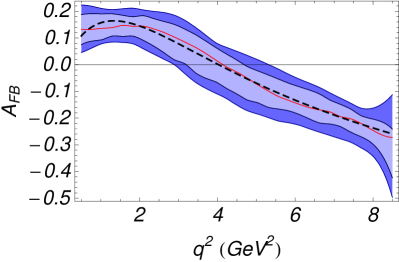
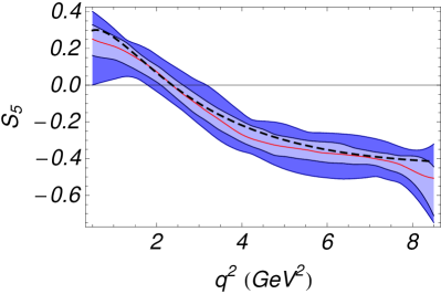
Figure 6: Projected experimental sensitivities to the observables $A_{\mathrm{FB}}$ and $S_{5}$ using an unbinned polynomial fit to 2$\mbox{\,fb}^{-1}$ of LHCb data in the range $q^{2}\in[0.5,8.5]\mathrm{\,Ge\kern-1.00006ptV}^{2}$. The dashed line shows the input distribution, while the solid line shows the median of an ensemble of 1200 fits. The light and dark contours show the estimated one and two $\sigma$ contours.

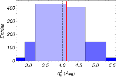
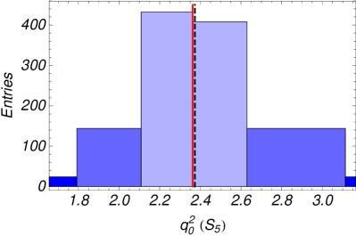
Figure 7: Projected experimental sensitivities to the zero-crossings of $A_{\mathrm{FB}}$ and $S_{5}$ using an unbinned polynomial fit to 2$\mbox{\,fb}^{-1}$ of LHCb data in the range $q^{2}\in[0.5,8.5]\mathrm{\,Ge\kern-1.00006ptV}^{2}$. The colour coding is the same as in Fig. 6.

Fig. 6 shows the projected experimental sensitivity to the full $A_{\mathrm{FB}}$ and $S_{5}$ distributions for 2$\mbox{\,fb}^{-1}$ of LHCb SM data. For ease of comparison with SM predictions, the zero-crossing point is extracted from the $q^{2}$ dependent distributions. These are shown in Fig. 7 for the same data sets as used in Fig. 6. The estimated $1\sigma$ uncertainties are shown in Tab. 9. As discussed in Ref. [17], the experimental uncertainty will scale approximately linearly with the gradient at the zero-crossing, leading to the large difference in estimated sensitivities seen for $q^{2}_{0}(A_{\mathrm{FB}})$ and $q^{2}_{0}(S_{5})$ in Tab. 9.

The difference in gradients between $A_{\mathrm{FB}}$ and $S_{5}$, seen in Fig. 5b for the majority of NP points, makes $q^{2}_{0}(S_{5})$ an attractive experimental target, assuming that any practical difficulties associated with the $\theta_{K^{*}}$ and $\phi$ decay angles can be overcome. We see that the relative steepness of the $S_{5}$ distribution is such that the experimental uncertainty on $q^{2}_{0}(S_{5})$ should be competitive with that on $q^{2}_{0}(A_{\mathrm{FB}})$ for the majority of the allowed regions of parameter space. For 0.5$\mbox{\,fb}^{-1}$, biases on the zero-crossing points become significant when using the unbinned analysis technique; however, it is likely that coarse estimates of $q^{2}_{0}(A_{\mathrm{FB}})$ and $q^{2}_{0}(S_{5})$ could be extracted even at this relatively small integrated luminosity using alternative techniques, such as those discussed in Ref. [18].

6 Impact of Future Measurements

The relative impact of the different analyses presented in Sec. 5 can be assessed by revisiting the parameter space exploration performed in Sec. 4. We are interested in how including these new measurements would affect the current constraints on parameter space. It is assumed that LHCb will make 2$\mbox{\,fb}^{-1}$ measurements of the observables $\left<A_{\mathrm{FB}}\right>_{\text{1-6}\mathrm{\,Ge\kern-0.70004ptV}^{2}}$, $\left<S_{5}\right>_{\text{1-6}\mathrm{\,Ge\kern-0.70004ptV}^{2}}$, $\left<F_{\mathrm{L}}\right>_{\text{1-6}\mathrm{\,Ge\kern-0.70004ptV}^{2}}$, $q^{2}_{0}(A_{\mathrm{FB}})$, and $q^{2}_{0}(S_{5})$ and that the resulting experimental uncertainties are symmetrized versions of those given in Tab. 9. In addition, we assume that the measured values of these observables are not affected by NP, and are as given in Tab. 8. The total $\chi^{2}$ for each point in parameter space is then updated to reflect these hypothetical SM measurements. Where individual measurements are superseded by LHCb measurements, they are replaced with no attempt at combination. However, other constraints, such as ${\cal B}(B\rightarrow X_{s}\gamma)$, are included as before. In this way the constraining power of each analysis can be compared.

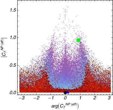
(a)  $\left<A_{\mathrm{FB}}\right>_{\text{1-6}\mathrm{\,Ge\kern-0.70004ptV}^{2}}$ & $q^{2}_{0}(A_{\mathrm{FB}})$

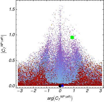
(b)  $\left<F_{\mathrm{L}}\right>_{\text{1-6}\mathrm{\,Ge\kern-0.70004ptV}^{2}}$

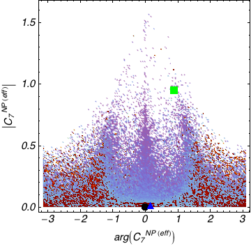
(c)  $\left<S_{5}\right>_{\text{1-6}\mathrm{\,Ge\kern-0.70004ptV}^{2}}$ & $q^{2}_{0}(S_{5})$

Figure 8: [Colour online] The relative impact of different proposed LHCb measurements after 2$\mbox{\,fb}^{-1}$ of integrated luminosity, assuming the SM, on the NP component of $C^{\mathrm{eff}}_{7}$. In each case the colour index has the same meaning as in Fig. 2.

Fig. 8 shows the relative impact of these measurements on the NP component of $C^{\mathrm{eff}}_{7}$. In Fig. 8a, SM values of $\left<A_{\mathrm{FB}}\right>_{\text{1-6}\mathrm{\,Ge\kern-0.70004ptV}^{2}}$ and $q^{2}_{0}(A_{\mathrm{FB}})$ are imposed with the estimated 2$\mbox{\,fb}^{-1}$ experimental sensitivities taken from Tab. 9. Fig. 8b shows the impact of $\left<F_{\mathrm{L}}\right>_{\text{1-6}\mathrm{\,Ge\kern-0.70004ptV}^{2}}$, while Fig. 8c shows the impact of both $\left<S_{5}\right>_{\text{1-6}\mathrm{\,Ge\kern-0.70004ptV}^{2}}$ and $q^{2}_{0}(S_{5})$ for the same LHCb integrated luminosity. These should be compared with the currently allowed $C^{\mathrm{eff}}_{7}$ parameter space shown in Fig. 2. The small statistical uncertainty found in Sec. 5 for $q^{2}_{0}(S_{5})$ provides a stringent constraint on parameter space. This emphasizes the importance of an early measurement of $S_{5}$, in addition to $A_{\mathrm{FB}}$ and $F_{\mathrm{L}}$.

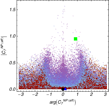
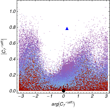
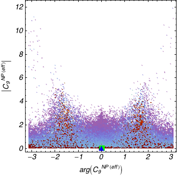
Figure 9: [Colour online] Allowed parameter space for the Wilson coefficients $C^{\mathrm{eff}}_{7}$, $C^{\prime\,\mathrm{eff}}_{7}$, $C^{\mathrm{eff}}_{9}$ and $C^{\prime\,\mathrm{eff}}_{10}$ after 2$\mbox{\,fb}^{-1}$ measurements at LHCb of $\left<F_{\mathrm{L}}\right>_{\text{1-6}\mathrm{\,Ge\kern-0.70004ptV}^{2}}$, $\left<A_{\mathrm{FB}}\right>_{\text{1-6}\mathrm{\,Ge\kern-0.70004ptV}^{2}}$, $q^{2}_{0}(A_{\mathrm{FB}})$, $\left<S_{5}\right>_{\text{1-6}\mathrm{\,Ge\kern-0.70004ptV}^{2}}$ and $q^{2}_{0}(S_{5})$, assuming the SM. The colour coding is the same as in Fig. 2.

Fig. 9 shows the combined effect of the measurement of the proposed observables, again assuming the SM and the estimated sensitivities from Tab. 9 for the NP contribution to the Wilson coefficients $C^{\mathrm{eff}}_{7}$, $C^{\prime\,\mathrm{eff}}_{7}$, $C^{\mathrm{eff}}_{9}$ and $C^{\prime\,\mathrm{eff}}_{10}$. The amount of parameter space left after these measurements would be significantly reduced, with most NP contributions excluded at the $1\sigma$ level unless there are large NP phases present. This again illustrates the importance of $C\!P$ observables as described in [14, 15]. The FBMSSM and GMSSM models from Sec. 3.2 could also be excluded at better than 95% confidence in this case.

7 Summary

A new next-to-leading order model of the decay $\kern 1.79993pt\overline{\kern-1.79993ptB}{}_{d}\rightarrow\kern 1.99997pt\overline{\kern-1.99997ptK}{}^{*0}\mu^{+}\mu^{-}$, that features QCD factorization corrections and full LCSR form factors, was presented. This includes an expression for the decay amplitude in terms of an updated set of auxiliary functions; these can be compared directly to the previous model, based on Ref. [22]. The auxiliary functions have been extended to include the effects of primed, scalar, and pseudoscalar operators, which may become important in certain NP scenarios.

The observables $A_{\mathrm{FB}}$, $F_{\mathrm{L}}$, and $S_{5}$ were identified as being promising for a relatively early measurement at the LHC, as they can be extracted as a function of $q^{2}$ by counting signal events in specific angular bins, using Eqs (20)–(22), and correspond to large features in the angular distribution. We also obtained a simple expression for $q^{2}_{0}(S_{5})$ at leading order, in terms of $C^{\mathrm{eff}}_{7}$, $C^{\prime\,\mathrm{eff}}_{7}$, and $C^{\mathrm{eff}}_{9}$, and showed that it has reduced hadronic form factor uncertainties in the large-recoil limit. Considering current experimental constraints leads to restrictions on the possible NP contributions to the Wilson coefficients. The allowed values of the $A_{\mathrm{FB}}$ and $S_{5}$ zero-crossing points, and the gradient of the $A_{\mathrm{FB}}$ and $S_{5}$ distributions at these points, were explored. The relative steepness of the $S_{5}$ distribution, even in the presence of NP, makes $q^{2}_{0}(S_{5})$ an experimentally attractive target, as it will lead to a smaller experimental uncertainty.

In order to investigate the impact of measuring the proposed observables on the NP contributions to the Wilson coefficients, and to compare their relative impact, we estimated their sensitivities at LHCb. We studied the sensitivity to the $q^{2}$ integrated values and zero-crossing points of $A_{\mathrm{FB}}$, $F_{\mathrm{L}}$, and $S_{5}$. The prospect of measuring $S_{5}$ and its zero-crossing at LHCb has not been previously explored.

Using a combination of $\left<F_{\mathrm{L}}\right>_{\text{1-6}\mathrm{\,Ge\kern-0.70004ptV}^{2}}$, $\left<A_{\mathrm{FB}}\right>_{\text{1-6}\mathrm{\,Ge\kern-0.70004ptV}^{2}}$, $q^{2}_{0}(A_{\mathrm{FB}})$, $\left<S_{5}\right>_{\text{1-6}\mathrm{\,Ge\kern-0.70004ptV}^{2}}$, and $q^{2}_{0}(S_{5})$, we showed that 2$\mbox{\,fb}^{-1}$ of LHCb data could greatly reduce the allowed parameter space. The contribution of $S_{5}$ to this is very significant and can, in part, be attributed to the small statistical uncertainty expected on $q^{2}_{0}(S_{5})$. We have also shown that if the decay is SM-like, the GMSSM and FBMSSM points considered would be ruled out by LHCb with 2$\mbox{\,fb}^{-1}$. We conclude by stressing that making measurements of $S_{5}$ and its zero-crossing would provide an interesting and complementary measurement to others currently planned. $\kern 1.79993pt\overline{\kern-1.79993ptB}{}_{d}\rightarrow\kern 1.99997pt\overline{\kern-1.99997ptK}{}^{*0}\mu^{+}\mu^{-}$ is a promising channel for constraining models or making a NP discovery. We look forward to the first LHC results for this decay.

Appendix

Appendix A Operator Basis

The effective Hamiltonian for $B_{d}\rightarrow K^{*0}\mu^{+}\mu^{-}$ can be expressed in terms of effective operators and Wilson coefficients as described in Sec. 2.2. We provide explicit expressions for a subset of these operators, which play a key role in the decay. Definitions for the remaining operators can be found in Ref. [14].

$${\mathcal{O}}_{7} =\frac{e}{g^{2}}\bar{m}_{b}(\bar{s}\sigma_{\mu\nu}P_{R}b)F^{\mu\nu}, {\mathcal{O}}_{7}^{\prime} =\frac{e}{g^{2}}\bar{m}_{b}(\bar{s}\sigma_{\mu\nu}P_{L}b)F^{\mu\nu},$$ (27)

$${\mathcal{O}}_{8} =\frac{1}{g}\bar{m}_{b}(\bar{s}\sigma_{\mu\nu}T^{a}P_{R}b)G^{\mu\nu\,a}, {\mathcal{O}}_{8}^{\prime} =\frac{1}{g}\bar{m}_{b}(\bar{s}\sigma_{\mu\nu}T^{a}P_{L}b)G^{\mu\nu\,a},$$ (28)

$${\mathcal{O}}_{9} =\frac{e^{2}}{g^{2}}(\bar{s}\gamma_{\mu}P_{L}b)(\bar{\mu}\gamma^{\mu}\mu), {\mathcal{O}}_{9}^{\prime} =\frac{e^{2}}{g^{2}}(\bar{s}\gamma_{\mu}P_{R}b)(\bar{\mu}\gamma^{\mu}\mu),$$ (29)

$${\mathcal{O}}_{10} =\frac{e^{2}}{g^{2}}(\bar{s}\gamma_{\mu}P_{L}b)(\bar{\mu}\gamma^{\mu}\gamma_{5}\mu), {\mathcal{O}}_{10}^{\prime} =\frac{e^{2}}{g^{2}}(\bar{s}\gamma_{\mu}P_{R}b)(\bar{\mu}\gamma^{\mu}\gamma_{5}\mu),$$ (30)

$${\mathcal{O}}_{S} =\frac{e^{2}}{16\pi^{2}}\bar{m}_{b}(\bar{s}P_{R}b)(\bar{\mu}\mu), {\mathcal{O}}_{S}^{\prime} =\frac{e^{2}}{16\pi^{2}}\bar{m}_{b}(\bar{s}P_{L}b)(\bar{\mu}\mu),$$ (31)

$${\mathcal{O}}_{P} =\frac{e^{2}}{16\pi^{2}}\bar{m}_{b}(\bar{s}P_{R}b)(\bar{\mu}\gamma_{5}\mu), {\mathcal{O}}_{P}^{\prime} =\frac{e^{2}}{16\pi^{2}}\bar{m}_{b}(\bar{s}P_{L}b)(\bar{\mu}\gamma_{5}\mu),$$ (32)

where $g$ is the strong coupling constant, e is the electron charge, $\overline{m}_{b}$ is the $b$ quark mass in the $\overline{\mathrm{MS}}$ scheme, as described in Sec. 2, and $P_{L,R}=(1\mp\gamma_{5})/2$.

Appendix B Angular Coefficients

Here we provide the relations between the angular coefficients, $I^{(s/c)}_{i}$, defined in Sec. 3.1 and the auxiliary functions defined in Eq. (8). We first express the $I^{(s/c)}_{i}$’s in terms of transversity amplitudes as in Ref. [15].

$$I_{1}^{s} =\frac{(2+\beta^{2})}{4}\left[|{A_{\perp}^{L}}|^{2}+|{A_{\parallel}^{L}}|^{2}+(L\rightarrow R)\right]+\frac{4m_{\mu}^{2}}{q^{2}}\text{Re}\left({A_{\perp}^{L}}{A_{\perp}^{R}}^{*}+{A_{\parallel}^{L}}{A_{\parallel}^{R}}^{*}\right)$$ (33)

$$I_{1}^{c} =|{A_{0}^{L}}|^{2}+|{A_{0}^{R}}|^{2}+\frac{4m_{\mu}^{2}}{q^{2}}\left[|A_{t}|^{2}+2\text{Re}({A_{0}^{L}}{A_{0}^{R}}^{*})\right]+\beta^{2}|A_{S}|^{2},$$ (34)

$$I_{2}^{s} =\frac{\beta^{2}}{4}\left[|{A_{\perp}^{L}}|^{2}+|{A_{\parallel}^{L}}|^{2}+(L\rightarrow R)\right],$$ (35)

$$I_{2}^{c} =-\beta^{2}\left[|{A_{0}^{L}}|^{2}+(L\rightarrow R)\right],$$ (36)

$$I_{3} =\frac{1}{2}\beta^{2}\left[|{A_{\perp}^{L}}|^{2}-|{A_{\parallel}^{L}}|^{2}+(L\rightarrow R)\right],$$ (37)

$$I_{4} =\frac{1}{\sqrt{2}}\beta^{2}\left[\text{Re}({A_{0}^{L}}{A_{\parallel}^{L}}^{*})+(L\rightarrow R)\right],$$ (38)

$$I_{5} =\sqrt{2}\beta\left[\text{Re}({A_{0}^{L}}{A_{\perp}^{L}}^{*})-(L\rightarrow R)-\frac{m_{\mu}}{\sqrt{q^{2}}}\,\text{Re}({A_{\parallel}^{L}}{A_{S}^{*}}+{A_{\parallel}^{R}}{A_{S}^{*}})\right],$$ (39)

$$I_{6}^{s} =2\beta\left[\text{Re}({A_{\parallel}^{L}}{A_{\perp}^{L}}^{*})-(L\rightarrow R)\right],$$ (40)

$$I_{6}^{c} =4\beta\frac{m_{\mu}}{\sqrt{q^{2}}}\,\text{Re}\left[{A_{0}^{L}}{A_{S}^{*}}+(L\rightarrow R)\right],$$ (41)

$$I_{7} =\sqrt{2}\beta\left[\text{Im}({A_{0}^{L}}{A_{\parallel}^{L}}^{*})-(L\rightarrow R)+\frac{m_{\mu}}{\sqrt{q^{2}}}\,{\text{Im}}({A_{\perp}^{L}}{A_{S}^{*}}+{A_{\perp}^{R}}{A_{S}^{*}})\right],$$ (42)

$$I_{8} =\frac{1}{\sqrt{2}}\beta^{2}\left[\text{Im}({A_{0}^{L}}{A_{\perp}^{L}}^{*})+(L\rightarrow R)\right],$$ (43)

$$I_{9} =\beta^{2}\left[\text{Im}({A_{\parallel}^{L}}^{*}{A_{\perp}^{L}})+(L\rightarrow R)\right].$$ (44)

These transversity amplitudes are projections of the decay amplitude onto various combinations of helicity states of the $K^{*}$ and the virtual gauge boson. The projections can be achieved by contracting $\mathcal{T}_{\mu}^{1/2}$ with the virtual gauge boson polarization vector. We use four basis vectors for the virtual gauge boson polarization vector corresponding to transverse ($\pm$), longtitudinal (0) and time-like (t) states, and three basis vectors for the virtual gauge boson polarization vector corresponding to transverse ($\pm$) and longtitudinal (0) states. One first extracts the helicity amplitudes $H_{+}$, $H_{-}$ and $H_{0}$ using the basis polarization vectors +,-,0 respectively for both the $K^{*}$ and the virtual gauge boson. $H_{t}$ is found by taking the longtitudinal polarization vector for the $K^{*}$ and the time-like polarization vector for the virtual gauge boson. Using the relations

$$A_{\perp/\parallel}=\frac{H_{+}\mp H_{-}}{\sqrt{2}}$$ (45)

and $A_{0}=H_{0}$, $A_{t}=H_{t}$, one then obtains expressions for the transversity amplitudes in terms of $A(q^{2})$ to $S(q^{2})$,

$$A^{i}_{\perp}(q^{2}) =\sqrt{2\,\lambda}\,N\,m_{B}\,c_{i}(q^{2})$$ (46)

$$A^{i}_{\parallel}(q^{2}) =-\sqrt{2}\,N\,m_{B}\,a_{i}(q^{2})$$ (47)

$$A^{i}_{0}(q^{2}) =\frac{N\,m_{B}}{\hat{m}_{K^{*}}\,\sqrt{\hat{q}^{2}}}\left(-\frac{1-\hat{m}_{K^{*}}^{2}-\hat{q}^{2}}{2}\,a_{i}(q^{2})+\lambda\,b_{i}(q^{2})\right)$$ (48)

$$A_{t}(q^{2}) =\frac{N\,m_{B}\,\sqrt{\lambda}}{\hat{m}_{K^{*}}\,\sqrt{\hat{q}^{2}}}\left(F(q^{2})-(1-\hat{m}_{K^{*}})G(q^{2})-\hat{q}^{2}H(q^{2})\right),$$ (49)

where $i=L/R$. We use the standard normalization and definitions following Ref. [12],

$$\beta= \sqrt{1-\frac{4m_{\mu}^{2}}{q^{2}}}$$ (50)

$$\lambda= 1+\hat{m}_{K^{*}}^{4}+\hat{q}^{4}-2\left(\hat{q}^{2}+\hat{m}_{K^{*}}^{2}\left(1+\hat{q}^{2}\right)\right)$$ (51)

$$N= \left(\frac{G_{F}^{2}\,\alpha^{2}}{3\cdot 2^{10}\pi^{5}\,m_{B}}|V_{ts}V^{*}_{tb}|^{2}q^{2}\,\lambda^{1/2}\,\beta\right)^{\frac{1}{2}},$$ (52)

where $\alpha$ is the electromagnetic coupling constant and $G_{F}$ is the Fermi constant. In the above definitions of the transversity amplitudes, the functions $a_{L/R}(q^{2})$, $b_{L/R}(q^{2})$, $c_{L/R}(q^{2})$, are analogous to those defined in Ref. [72],

$$a_{L/R}(q^{2}) =B(q^{2})\mp F(q^{2}),$$ (53)

$$b_{L/R}(q^{2}) =\frac{1}{2}\left(C(q^{2})\mp G(q^{2})\right),$$ (54)

$$c_{L/R}(q^{2}) =\frac{1}{2}\left(A(q^{2})\mp E(q^{2})\right).$$ (55)

Using the above it is possible to compare the predictions of Eqs (8) to the standard results in the literature, and we agree with Ref. [15].

References

- [1] T. Hurth, Status of SM calculations of transitions, Int. J. Mod. Phys. A22 (2007) 1781–1795 [hep-ph/0703226]
- [2] B. Grinstein and D. Pirjol, Precise determination from exclusive B decays: Controlling the long-distance effects, Phys. Rev. D70 (2004) 114005 [hep-ph/0404250]
- [3] BELLE Collaboration, A. Ishikawa et. al., Observation of the electroweak penguin decay , Phys. Rev. Lett. 91 (2003) 261601 [hep-ex/0308044]
- [4] BELLE Collaboration, A. Ishikawa et. al., Measurement of forward-backward asymmetry and Wilson coefficients in , Phys. Rev. Lett. 96 (2006) 251801 [hep-ex/0603018]
- [5] BABAR Collaboration, B. Aubert et. al., Measurements of branching fractions, rate asymmetries, and angular distributions in the rare decays and , Phys. Rev. D73 (2006) 092001 [hep-ex/0604007]
- [6] BABAR Collaboration, B. Aubert et. al., Angular distributions in the decays , Phys. Rev. D79 (2009) 031102 [0804.4412]
- [7] BABAR Collaboration, B. Aubert et. al., Direct , lepton flavor and isospin asymmetries in the decays , Phys. Rev. Lett. 102 (2009) 091803 [0807.4119]
- [8] BELLE Collaboration, J. T. Wei et. al., Measurement of the differential branching fraction and forward-backword asymmetry for , Phys. Rev. Lett. 103 (2009) 171801 [0904.0770]
- [9] CDF Collaboration, H. Miyake. Talk at HCP2009, 16-20.11.2009, Evian, France. PoS(HCP2009)033
- [10] A. Ali, T. Mannel and T. Morozumi, Forward backward asymmetry of dilepton angular distribution in the decay , Phys. Lett. B273 (1991) 505--512
- [11] G. Burdman, Short distance coefficients and the vanishing of the lepton asymmetry in , Phys. Rev. D57 (1998) 4254--4257 [hep-ph/9710550]
- [12] F. Kruger and J. Matias, Probing new physics via the transverse amplitudes of at large recoil, Phys. Rev. D71 (2005) 094009 [hep-ph/0502060]
- [13] U. Egede, T. Hurth, J. Matias, M. Ramon and W. Reece, New observables in the decay mode , JHEP 11 (2008) 032 [0807.2589]
- [14] C. Bobeth, G. Hiller and G. Piranishvili, CP asymmetries in and untagged decays at NLO, JHEP 07 (2008) 106 [0805.2525]
- [15] W. Altmannshofer et. al., Symmetries and asymmetries of decays in the standard model and beyond, JHEP 01 (2009) 019 [0811.1214]
- [16] A. Bharucha, : SM and Beyond, 0905.1289
- [17] W. Reece and U. Egede, ‘‘Performing the full angular analysis of at LHCb.’’ CERN-LHCb-2008-041
- [18] J. Dickens, V. Gibson, C. Lazzeroni and M. Patel, ‘‘A study of the sensitivity to the forward-backward asymmetry in decays at LHCb.’’ CERN-LHCb-2007-039
- [19] F. Jansen, N. Serra, G. Y. Smit and N. Tuning, ‘‘Determination of the forward-backward asymmetry in the decay with an unbinned counting analysis.’’ CERN-LHCb-2009-003
- [20] U. Egede, ‘‘Angular correlations in the decay.’’ CERN-LHCb-2007-057
- [21] LHCb Collaboration, A. A. Alves et. al., The LHCb Detector at the LHC, JINST 3 (2008) S08005
- [22] A. Ali, P. Ball, L. T. Handoko and G. Hiller, A comparative study of the decays in Standard Model and supersymmetric theories, Phys. Rev. D61 (2000) 074024 [hep-ph/9910221]
- [23] D. J. Lange, The EvtGen particle decay simulation package, Nucl. Instrum. Meth. A462 (2001) 152--155
- [24] Source code available from https://svnweb.cern.ch/trac/evtbtokstmumu.
- [25] G. Buchalla, A. J. Buras and M. E. Lautenbacher, Weak decays beyond leading logarithms, Rev. Mod. Phys. 68 (1996) 1125--1144 [hep-ph/9512380]
- [26] C. Bobeth, A. J. Buras and T. Ewerth, in the MSSM at NNLO, Nucl. Phys. B713 (2005) 522--554 [hep-ph/0409293]
- [27] C. Bobeth, T. Ewerth, F. Kruger and J. Urban, Analysis of neutral Higgs-boson contributions to the decays and , Phys. Rev. D64 (2001) 074014 [hep-ph/0104284]
- [28] P. Gambino, M. Gorbahn and U. Haisch, Anomalous dimension matrix for radiative and rare semileptonic decays up to three loops, Nucl. Phys. B673 (2003) 238--262 [hep-ph/0306079]
- [29] M. Gorbahn and U. Haisch, Effective Hamiltonian for non-leptonic decays at NNLO in QCD, Nucl. Phys. B713 (2005) 291--332 [hep-ph/0411071]
- [30] M. Gorbahn, U. Haisch and M. Misiak, Three–loop mixing of dipole operators, Phys. Rev. Lett. 95 (2005) 102004 [hep-ph/0504194]
- [31] M. Beneke, T. Feldmann and D. Seidel, Systematic approach to exclusive decays, Nucl. Phys. B612 (2001) 25--58 [hep-ph/0106067]
- [32] P. Ball and R. Zwicky, , , , decay form factors from light-cone sum rules reexamined, Phys. Rev. D71 (2005) 014029 [hep-ph/0412079]
- [33] D. Becirevic, V. Lubicz and F. Mescia, An estimate of the form factor, Nucl. Phys. B769 (2007) 31--43 [hep-ph/0611295]
- [34] M. A. Shifman, A. I. Vainshtein and V. I. Zakharov, QCD and Resonance Physics. Sum Rules, Nucl. Phys. B147 (1979) 385--447
- [35] P. Colangelo and A. Khodjamirian, QCD sum rules, a modern perspective, hep-ph/0010175. In At the frontier of particle physics: Handbook of QCD, World Scientific (2001) 2188p.
- [36] P. Ball. Private communication, 2009
- [37] J. Charles, A. Le Yaouanc, L. Oliver, O. Pene and J. C. Raynal, Heavy-to-light form factors in the heavy mass to large energy limit of QCD, Phys. Rev. D60 (1999) 014001 [hep-ph/9812358]
- [38] J. Charles, A. Le Yaouanc, L. Oliver, O. Pene and J. C. Raynal, Heavy–to–light form factors in the final hadron large energy limit: Covariant quark model approach, Phys. Lett. B451 (1999) 187 [hep-ph/9901378]
- [39] M. J. Dugan and B. Grinstein, QCD basis for factorization in decays of heavy mesons, Phys. Lett. B255 (1991) 583--588
- [40] M. Beneke and T. Feldmann, Symmetry–breaking corrections to heavy–to–light meson form factors at large recoil, Nucl. Phys. B592 (2001) 3--34 [hep-ph/0008255]
- [41] M. Beneke, T. Feldmann and D. Seidel, Exclusive radiative and electroweak and penguin decays at NLO, Eur. Phys. J. C41 (2005) 173--188 [hep-ph/0412400]
- [42] Q.-S. Yan, C.-S. Huang, W. Liao and S.-H. Zhu, Exclusive semileptonic rare decays in supersymmetric theories, Phys. Rev. D62 (2000) 094023 [hep-ph/0004262]
- [43] Particle Data Group Collaboration, C. Amsler et. al., Review of particle physics, Phys. Lett. B667 (2008) 1
- [44] A. Signer, The charm quark mass from non-relativistic sum rules, Phys. Lett. B672 (2009) 333--338 [0810.1152]
- [45] A. Pineda and A. Signer, Renormalization group improved sum rule analysis for the bottom quark mass, Phys. Rev. D73 (2006) 111501 [hep-ph/0601185]
- [46] Tevatron Electroweak Working Group Collaboration, Combination of CDF and D0 results on the mass of the top quark, 0808.1089
- [47] M. Beneke, A quark mass definition adequate for threshold problems, Phys. Lett. B434 (1998) 115--125 [hep-ph/9804241]
- [48] T. Onogi, Heavy flavor physics from lattice QCD, PoS LAT2006 (2006) 017 [hep-lat/0610115]
- [49] P. Ball, V. M. Braun and A. Lenz, Twist-4 distribution amplitudes of the K∗ and mesons in QCD, JHEP 08 (2007) 090 [0707.1201]
- [50] P. Ball and R. Zwicky, from , JHEP 04 (2006) 046 [hep-ph/0603232]
- [51] E. Lunghi and J. Matias, Huge right-handed current effects in in supersymmetry, JHEP 04 (2007) 058 [hep-ph/0612166]
- [52] B. Grinstein and D. Pirjol, The forward-backward asymmetry in decays, Phys. Rev. D73 (2006) 094027 [hep-ph/0505155]
- [53] W. Altmannshofer, A. J. Buras and P. Paradisi, Low energy probes of violation in a flavor blind MSSM, Phys. Lett. B669 (2008) 239--245 [0808.0707]
- [54] E. Gabrielli and S. Khalil, On the decays in general supersymmetric models, Phys. Lett. B530 (2002) 133--141 [hep-ph/0201049]
- [55] HPQCD Collaboration, A. Gray et. al., The B Meson Decay Constant from Unquenched Lattice QCD, Phys. Rev. Lett. 95 (2005) 212001 [hep-lat/0507015]
- [56] Heavy Flavor Averaging Group (HFAG) Collaboration, E. Barberio et. al., Averages of B–hadron properties at the end of 2006, 0704.3575 [hep-ex]
- [57] CDF Collaboration, T. Aaltonen et. al., Search for and decays with of collisions, Phys. Rev. Lett. 100 (2008) 101802 [0712.1708]
- [58] CDF Collaboration, ‘‘Search for and decays with of collisions.’’ CDF Public Note 9892, 2009
- [59] BABAR Collaboration, B. Aubert et. al., Measurement of the branching fraction with a sum over exclusive modes, Phys. Rev. Lett. 93 (2004) 081802 [hep-ex/0404006]
- [60] BELLE Collaboration, M. Iwasaki et. al., Improved measurement of the electroweak penguin process , Phys. Rev. D72 (2005) 092005 [hep-ex/0503044]
- [61] G. Hiller and F. Kruger, More model-independent analysis of processes, Phys. Rev. D69 (2004) 074020 [hep-ph/0310219]
- [62] A. Ghinculov, T. Hurth, G. Isidori and Y. P. Yao, The rare decay to NNLL precision for arbitrary dilepton invariant mass, Nucl. Phys. B685 (2004) 351--392 [hep-ph/0312128]
- [63] D. Guetta and E. Nardi, Searching for new physics in rare decays, Phys. Rev. D58 (1998) 012001 [hep-ph/9707371]
- [64] P. Gambino and P. Giordano, Normalizing inclusive rare B decays, Phys. Lett. B669 (2008) 69--73 [0805.0271]
- [65] M. Misiak et. al., The first estimate of at , Phys. Rev. Lett. 98 (2007) 022002 [hep-ph/0609232]
- [66] M. Misiak, QCD calculations of radiative decays, 2008. Talk at HQL2008, 5-9.06.2008, Melbourne, Australia, 0808.3134
- [67] P. Ball and R. Zwicky, Time-dependent CP asymmetry in as a (quasi) null test of the standard model, Phys. Lett. B642 (2006) 478--486 [hep-ph/0609037]
- [68] P. Ball, G. W. Jones and R. Zwicky, beyond QCD factorisation, Phys. Rev. D75 (2007) 054004 [hep-ph/0612081]
- [69] M. Bauer, S. Casagrande, U. Haisch and M. Neubert, Flavor physics in the Randall-Sundrum model: II. tree- level weak-interaction processes, 0912.1625
- [70] LHCb Collaboration, B. Adeva et. al., Roadmap for selected key measurements of LHCb, 0912.4179
- [71] M. Patel and H. Skottowe, ‘‘A Fisher discriminant selection for .’’ CERN-LHCb-2009-009
- [72] C. S. Kim, Y. G. Kim, C. Lu and T. Morozumi, Azimuthal angle distribution in at low invariant region, Phys. Rev. D62 (2000) 034013 [hep-ph/0001151]