Influence of nonlinear dissipation and external perturbations onto transition scenarious to chaos in Lorenz-Haken system
Abstract
We study an influence of nonlinear dissipation and external perturbations onto transition scenarious to chaos in Lorenz-Haken system. It will be show that varying in external potential parameters values leads to parameters domain formation of chaos realization. In the modified Lorenz-Haken system transitions from regular to chaotic dynamics can be of Ruelle-Takens scenario, Feigenbaum scenario, or through intermittency.
1 Introduction
One of the most actual tasks in the theory of nonlinear dynamical systems is a setting of chaotic regime generation conditions and defining possibilities of chaos control [1, 2]. It is well known, that in physical applications for a transition from chaotic to periodic mode in multicomponent systems different mechanisms are used. For example, in laser physics they are negative feedback [3], angle between two crystals which are entered to the Fabry-Perot cavity [4], full feedback intensity [1], intensity of activating [5] (see [6] and citations therein). In this connection, from the theoretical point of view, an actual task is to establish of chaos control and to determine transition characters between chaotic and regular dynamics.
The main goal of this work is to study an influence of two additional nonlinearityes that arise up in the chaotic system as a result of different physical processes onto transitions character between regular and chaotic dynamics. We shall consider a modified Lorenz-Haken model which self-consistently can describes, for example, optical bistable systems [7], systems of defects are in a solid [8, 9], etc. Due to condition of commensurability for all three modes relaxation times we shall set domains of system parameters of chaos realization with a help of maximal Lyapunov exponents approach. We shall obtain two different strange chaotic attractors and shall set possible transitions to chaotic dynamics.
The paper is organized in the following manner. In Section 2 we present a model of our system incorporating a nonlinear dissipation external perturbation terms. Section 3 is devoted to the consideration of conditions for transition to chaotic regime and to determination the main characteristics of strange chaotic attractor. The main results and prospects for the future are presented in the Conclusions.
2 A model of a chaotic system
A Lorenz-Haken model can be written in a form [7]:
| (1) |
Here a point means a derivative in time , , – relaxation times of an order parameter , a conjugating field and a control parameter , accordingly; , , – positive feed-back constants; – pump intensity, measures the influence of environment. First elements in the left hand of the systems (1) take into account dissipation effects, peculiar to the synergetic systems. Connection between the order parameter and conjugating field is linear (first equation), in that time as an evolution of the conjugating field , and control parameter sets due to nonlinear feed-backs relations (second and third equations, respectively). Principally that positive feed-backs which are provided by constant and result in an increase in conjugating field. These positive feed-backs are compensated by negative one due to principle of Le-Shatel’e. As a result one has decreasing in control parameter (see third equation in Eq.(1)).
Let us start the analysis of the system (1) with passing to dimensionless variables. Such transition is arrived due to measuring of time , order parameter , conjugating field , and control parameter in the followings units:
In this time, dropping indexes, the system (1) becomes a form
| (2) |
where , . The system (2) is written in supposition of linear dependence for order parameter relaxation time as . However, most real physical systems are characterized by the nonlinear relaxation processes. In this connection let us suppose that the order parameter relaxation time increasing with increase in order parameter due to relation [10]:
| (3) |
where – positive constant which play a role of an dissipation intensity. From Eq.(3) it is seen that relaxation time is independent of order parameter sign. Except for that, relation (3) has practical application namely, it designs the action of optical filter, entered into the Fabry-Perot cavity of optically bistable system (for example solid-state laser). Such acting provides establishment of the stable periodic radiation (or time dissipative structure realization) [11]. Using a dependence (3), first equation of (2) is generalized by an additional nonlinear term .
If one consider system in external field, then one need to take into consideration external perturbations. In this article we shall model such perturbations by the external potential . Due to the standard catastrophe theory such potential is given by three types of catastrophes [12]. In general case one has
| (4) |
where , , , , – parameters of the theory. For a catastrophe one has , for a catastrophe : and for a catastrophe : . The modified Lorenz-Haken system has the form
| (5) |
where we suppose and . Variation in parameters of and can to induce changing of the attractor topology in phase space.
3 Chaos in a modified Lorenz-Haken system
The system Eq.(5) with nonlinear dependence of order parameter relaxation time versus order parameter in a form (3) () but with absence of additional perturbations () was considered in [11]. It was shown that in such a case the semirestricted domain of system parameters (pump intensity and dissipation intensity ) for dissipative structure realization is formed. It was set that in a case of linear dependence for order parameter relaxation time versus its values () chaotic regime is not realize. In addition, it was found the chaos domain, and it was determined conditions of chaos control. Finally it was defined fractal and statistical properties of corresponding chaotic strange attractor.
The main goal in this work is to study an influence of external perturbation, on a regimes of transition to chaos in Lorenz-Haken system, generalized by nonlinear relaxation time of order parameter in a form (3). For external perturbations we will use a potential of the fold catastrophe , i.e. . To indicate a chaotic dynamic we shall use a method of Lyapunov exponents which is provided by a Benettin algorithm [13]. Due to this algorithm each of Lyaponov exponent (number is defined by dimension of corresponding phase space) determines a speed of convergence/divergence of any two initially nearby trajectories in a fixed direction in corresponding phase space, starting from points and . The divergence/convergence of such trajectories is given by the dependence , where is a maximal (global) Lyapunov exponent, which is defined due to relation [13]
Here one takes into account an upper limit and is a norm; ; – full time. One can conclude that in a case , , and accordingly all of phase trajectories will coincide to fixed point (stable node or stable focus). At , and , phase trajectories will lie down on a stable limit circle (dissipative structure). If , and , a dynamics of the system is chaotic. A Lyapunov map of the modified Lorenz-Haken system (5) at and is shown in Fig.1.
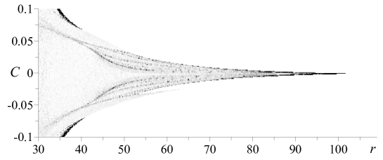
Here by gradation of grey color the value of maximal (global) Lyapunov exponent is shown versus pump intensity and parameter of an external potential . White color determines the domains of stable system behaviour (phase space is characterized by a fixed point – stable node or a stable focus). Grey color marks the domains of time dissipative structure existence (more dark domains correspond to the larger number of oscillation periods). Domains of chaos are shown by a black colour. From Fig.1 it is seen, that in a case of nonlinear term absence in the external potential the existence of the chaotic mode requires the large values of pump intensity. In case the chaotic mode exists at .
Let us analyze a picture of dynamical regimes reconstruction for the system (5) with and in detail. Lyapunov map and corresponding dependence of maximal Lyapunov exponent versus pump intensity at fixed value of dissipation intensity with characteristic phase portraits are shown in Fig.2.
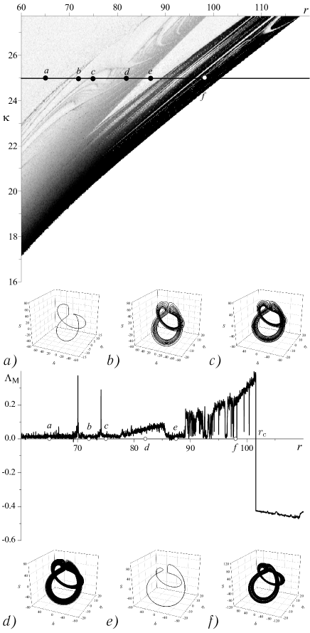

Here due to earlier denoted scenario values of maximal Lyapunov exponent are presented by gradation of grey color versus pump intensity and dissipation intensity. It is necessary to note that dark curves (between a and b, b and c in a Lyapunov map) in the domain of dissipation structure existence (grey area) are determine the parameters values of doubling period bifurcation. Below the map there is a dependence of maximal Lyapunov exponent versus pump intensity at , and . A presence of two pronounced peaks in the domain of zero values of maximal Lyapunov exponent (fluctuations around a zero are connected with an error of numeral solution of systems (5)) determines the points of doubling period bifurcation. Corresponding phase portraits illustrating dissipative structure with one, and periods are shown with the help of insertions a), b) and c), accordingly. It is principally, that as transition from a) to b), as transition from b) to c) characterizes by appearance of a few additional harmonics. As it is seen from dependence in a point d maximal Lyapunov exponent has positive value and phase space is characterized by the irregular behaviour of trajectory. Increasing in pump intensity leads to dissipative structure formation with one period (cf. phase portraits d) and e)). Next increasing in leads to positive values of and phase space is characterized by chaos existence (corresponding phase portrait is shown with the help of insertion f). So, one can conclude that at , and with an increase in pump intensity a transition to chaotic regime occurs due to Ruelle-Takens scenario, when only negligible number of doubling period bifurcation leads to chaos [14]. With a decreasing in (from to ) maximal Lyapunov exponent takes positive value at in spontaneous manner. Corresponding transition to chaos takes a place through intermittency [15].
Next, let us consider the domain of chaos, shown in Fig.1 at . Lyapunov map at and is shown in Fig.3. Below the map as well as in previous case a dependence of maximal Lyapunov exponent versus pump intensity at , and and corresponding phase portraits are shown. Unlike to the previous case here with an increase in pump intensity a successive complication of attractor due to doubling period bifurcation is observed (see corresponding phase portraits in points a, b, c, d and e). Thus, in such a case (, and ) an increasing in results to transition to chaos due to Feigenbaum scenario [14]. Chaotic attractor is shown with the help of insertion f). As in a previous case a decrease in leads to transition to chaos at through intermittency [15].
It is well known that dynamical systems can realize four types of attractors in phase space, namely: non chaotic non strange attractor, chaotic non strange attractor, strange non chaotic attractor and chaotic strange attractor. So, for chaotic attractor one has () and for an strange one – fractal dimension of an attractor is fractional. In [16] it was shown that the fractal dimension of an attractor which is realized in the dynamical system, is determined with the help of Lyapunov exponents due to relation
where is a minimal Lyapunov exponent. Thus, for considered attractor in a point f at , , and (see Fig.2) one has: , and, accordingly, . For the attractor at , , and (see Fig.3) one has , and accordingly, . Thus, attractors in Fig.2f and Fig.3f are strange and chaotic.
4 Conclusions
We have studied an influence of nonlinear dissipation and external perturbations onto transition scenarious to chaos in Lorenz-Haken system. Dissipation processes are defined due to nonlinear dependence of order parameter relaxation time versus its values. External perturbations are modeled by a potential of fold catastrophe .
From a physical view point we have considered an absorptive optical bistability system [7]. At that time used nonlinear dissipation relation related to the possibility of the additional medium in the Fabry-Perot cavity (phthalocyanine fluid, gases , , and [7]) to absorbing signals with weak intensities. Meanwhile, external perturbations model an influence of optical modulator which sets additional interphotons interaction processes in the Fabry-Perot cavity.
We have considered a case of commensurability of relaxation times for order parameter, conjugated field and control parameter. It has been shown that varying in external potential parameters values leads to parameters domain formation with and with by order of magnitude greater than of chaos realization. In considered system transitions from regular to chaotic dynamics can be of Ruelle-Takens scenario, Feigenbaum scenario, or through intermittency.
References
- [1] J.N.Blakely, L.Illing, D.J.Gauthier, High-speed chaos in an optical feedback system with flexible timescales, IEEE Journ. of quant. el.,40,299-306(2004).
- [2] G.D.Van Wiggeren, R.Roy, Communication with dynamically fluctuating states of light polarization, Phys. Rev. Lett., 88,097903(4)(2002).
- [3] R.Meucci, M.Ciofini, R.Abbate, Suppressing chaos in lasers by negative feedback, Phys. Rev. E, 53,R5537-R5540(1996).
- [4] C.Bracikowski, R.Roy, Chaos in a multimode solid-state laser system, Chaos, 1,49-64(1991).
- [5] Z.Gills, C.Iwata, R.Roy, Tracking unstable steady states: extending the stability regime of a multimode laser system, Phys. Rev. Lett., 69,3169-3173(1992).
- [6] S.Boccaleti [et al.], The control of chaos: theory and applications, Physics reports, 392,103-197(2000).
- [7] H.Haken, Synergetics, Springer,New Yokr,1983.
- [8] A.I. Olemskoi, Theory of structure transformations in non-equilibrium condensed matter, Nova Science publishers inc.,New York,1999.
- [9] D.O.Kharchenko, I.A.Knyaz, Fluctuation-induced reconstruction of defect structure (G.O.Puchkovska, T.A.Gavrilko, O.I.Lizengevich eds.), Proc. of SPIE 5507,17-25(2004).
- [10] A.I.Olemskoi, A.V.Khomenko, Three-parametric kinetic of phase transition, JETP, 110,2144-2167(1996).
- [11] E.D.Belokolos, V.O.Kharchenko, D.O.Kharchenko, Chaos in a generalized Lorenz system, Chaos, Solitons and Fractals, 41,2595-2605(2009).
- [12] T.Poston, I.N.Stewart, Catastrophe Theory and Its Applications, Pitman,London,1978.
- [13] G.Benettin [et al.], Lyapunov characteristic exponents for smooth dynamical systems and for Hamiltonian systems: P.I: Theory. P.II: Numerical application, Meccanica, 15,9-30(1980).
- [14] H.G.Shuster, Deterministic Chaos, An Introduction, Physik-Verlag,Weinheim,1984.
- [15] R.Z.Sagdeev, D.A.Usikov, G.M.Zaslavskii, Nonlinear physicks: from the pendulum to turbulemce and chaos, Harwood Academic,Chur,1988).
- [16] J.C.Sprott Chaos Time-Series Analysis, Oxford,Oxford University Press,2003.