Anderson Transition in Disordered Bilayer Graphene

Abstract

Employing the Kernel Polynomial method (KPM), we study the electronic properties of the graphene bilayers in the presence of diagonal disorder, within the tight-binding approximation. The KPM method enables us to calculate local density of states (LDOS) without need to exactly diagonalize the Hamiltonian. We use the geometrical averaging of the LDOS’s at different lattice sites as a criterion to distinguish the localized states from extended ones. We find that bilayer graphene undergoes Anderson metal-insulator transition at a critical value of disorder strength.

I introduction

Graphene (the 2D allotrope of carbon with honeycomb structure) has attracted tremendous attraction since its isolation by Novoselov et al Novoselov2 . Some of the features that makes graphene distinct from previously known materials are properties such as, possibility to control the charge carrier types from hole to electron in the same sample by a gate voltage, high mobility of charge carriers (about two orders of magnitude larger than the best silicon based semiconductors), anomalous integer Quantum Hall effect (IQHE) at room temperature  NetoRMP ; QHE . Among them, the high mobility of carriers which is due to the vanishing of back-scatterings, makes graphene favorable in fabrication of carbon-based electronic devices.

The spectral and transport properties of graphene are well described within the tight-binding approximation. In this model the two upper energy bands, which are due to the $\pi$ and $\pi^{*}$ bonds of $p_{z}$ orbitals normal to the honeycomb lattice plane, touch each other with a linear dispersion at the corners of the Brillouin zone (the so called $K$-points) Wallace . In this picture graphene is a semi-metal whose low energy excitations are massless fermions propagating with Fermi velocity ($v_{F}$) of about $1/300$ times the light speed. These excitations are called Dirac-fermions, which, along with strong stability of graphene structure (which is related to the in plane $\sigma$ bonds), are responsible for the odd properties of graphene NetoRMP .

Employing graphene in electronic devices requires the opening of gap in its electronic spectrum. This can be done by constraining its geometry either to graphene nano-ribbons or quantum-dots. However these methods affect the electronic transport because of formation of rough edges and also enhancement of the Coulomb blockade effects in the small size structures Han . Moreover, by reducingthe size and symmetry, the selection rules tend to get more restrictive, hence reducing the possible conduction channels. Nevertheless, it has been shown that by applying an electric field normal to a graphene bilayer a gap can be opened whose magnitude is proportional to the intensity of the applied electric field  McCann ; McCann1 . The size of gap can be as large as 0.1-0.3 eV, thereby making the bilayer graphene an attractive candidate in carbon-based transistors  Nilsson .

The graphene bilayer consists of two layers of carbon atoms in honeycomb structure placed on top of each other, making the Bernal stacking  Nilsson1 . In this stacking the upper layer is rotated 60 degree relative to the lower one, in such a way that the atoms in one sublattice, i.e $A_{1}$ and $A_{2}$, are on the top of each other while the atoms of the $B$-sublattice in upper layer are placed on the top of the hallow center of hexagons of the lower layer . In the absence of external perpendicular electric field the band structure of graphene bilayer consists of four bands, arising from the $\pi$-bonding between $p_{z}$ orbitals. Two of these bands touch each other at zero energy with a quadratic dispersion, and so give rise to the massive quasi-particles also called chiral fermions McCann . The other two bands are separated by energy scale corresponding to the inter-plane hopping energy, $t_{\bot}$; one laying below the zero energy and the other above it. The electronic structures of bilayer as well as multilayer graphene have been extensively investigated recently McCann ; Nilsson ; Berger1 ; Berger2 ; Nilsson2 ; Novoselov1 ; Koshino .

The single and double layer samples of graphene can be grown with high crystalline quality. However there are inevitable sources of disorder which may affect the electronic transport in the fabricated samples. Typical forms of disorder includes surface ripples, topological defects, vacancies, ad-atoms, charge impurities and polarization field of the substrate. Scaling theory of localization predicts that all the electronic states are localized in two-dimensional systems, once smallest amount of disorder is introduced AndersonLocalization . According to this theory, the single and bilayer of graphene are expected to be insulators at zero temperature. However theoretical as well as experimental studies show that both single and bilayer graphene, have a minimum conductivity of the order of conductance quantum ($e^{2}/h$) at the charge neutrality point  Fradkin . It is also shown that the minimum conductivity is at least twice larger in the bilayer graphene  Koshino ; Snyman . These results are in contrast to prediction of the scaling theory of localization and motivate us to study the localization properties of electronic states in graphene systems. In our previous work, we investigate the the single layer graphene in the presence of on-site disorder by using the numerically powerful approach of KPM amini . There, we found that disordered graphene mono-layer shows Anderson transition at a critical value of disorder intensity which is of the order of bandwidth. Our calculation also brought an unusual theoretical prediction according to which, the localization starts from the states near the Dirac points and spreads toward the band edges by increasing the amount of disorder amini . This type of metal-insulator transition driven by short range diagonal disorder due to neutral impurities, was experimentally verified in Hydrogen dozed graphene by angular resolved photoemission experiment Horn .

In this paper we investigate the localization properties of the electronic states in bilayer graphene in presence of diagonal disorder. We consider minimal coupling between two layers of graphene, that is, we take into account only the hopping between $A_{1}$ and $A_{2}$ sublattices. Here we use the kernel polynomial method (KPM) Weisse , which consists in the expansion of various spectral functions in terms of a complete set of polynomials. We calculate different local density of states (LDOS), from which we introduce a quantity for distinguishing the localized states from extended ones. The CPU time in this method grows proportional to square of the system size, enabling us to study large lattice sizes in a moderate time.

II Model Hamiltonian

As was mentioned before, we use a minimal tight-binding model for describing the low energy transport properties of the graphene bilayer. In this model we consider only the hopping between the $p_{z}$ orbitals residing on the nearest neighbor sites. In this picture the two layers are assumed to communicate only through the hopping among $A_{1}$ and $A_{2}$ sublattices in the Bernal stacking. The Hamiltonian can be written as:

$$H= - t\sum_{m=1}^{2}\sum_{\langle i,j\rangle}{a_{m,i}^{\dagger}b_{m,j}+h.c.}$$

$$- t_{\perp}\sum_{i}{a_{1,i}^{\dagger}a_{2,i}+h.c.}$$

$$+ \sum_{m=1}^{2}\sum_{i}\epsilon^{a}_{m,i}a_{m,i}^{\dagger}a_{m,i}+\epsilon^{b}_{m,i}b_{m,i}^{\dagger}b_{m,i},$$

in which $a_{m,i}^{\dagger}$($a_{m,i}$) creates (annihilates) a $p_{z}$-electron at site $(m,i)$ on the sublattice A, with $m=1,2$, where $m$ is the index of layers and $i$ labels the sites on each A-sublattice in given layer. Similarly, $b_{m,i}^{\dagger}$ and $b_{m,i}$ are the corresponding creation and annihilation operators in the B-sublattices of the two layers. Here, $t$ denotes the intra-plane hopping integral between the nearest neighbors and $t_{\perp}$ is the inter-plane hopping amplitude between two layers. Empirical estimates of the hopping terms are $t\sim 3.16$ eV, and $t_{\perp}\sim 0.39$ eV Toy ; Misu . There are further inter-plane couplings, where for simplicity we ignore them in our study. Also, $\epsilon^{a}_{m,i}$ and $\epsilon^{b}_{m,i}$ in the last term denote the on-site energies at A and B sublattices on each layer, respectively. To introduce disorder on the model, we choose the on-site energies randomly from a uniform distribution in the interval $[-\frac{W}{2},\frac{W}{2}]$. This is the so called Anderson model with spatially uncorrelated diagonal disorder in which $W$ is a measure for the intensity of disorder. Hereafter, we assume the unit of energy to be set by $t$.

III Kernel Polynomial Method

Local density of states (LDOS), denoted by $\rho_{i}(E)$, is a quantity that measures the contribution of a given lattice site $i$ in total density of energy states of the lattice in the interval $[E,E+dE]$, and is defined by the following relation:

$${\rho_{i}}(E)=\sum_{n=1}^{N}|\langle i|E_{n}\rangle|^{2}\delta(E-E_{n}),$$ (2)

in which $|E_{n}\rangle$ is the energy eigenvector corresponding to energy eigenvalue $E_{n}$. $|\langle i|E_{n}\rangle|^{2}$ in Eq. (2) is the probability of finding an electron with energy $E_{n}$ on the site $i$, which in the absence of disorder is the same for all lattice sites as a result of translational invariance. However for localized states encountered in disordered systems, this probability drastically varies over the system. If the Hamiltonian possesses an extended eigenstate with the eigenvalue between $E$ and $E+dE$, then all sites are comparably likely to be present in this state, while for a localized state only a limited number of sites have appreciable probability of being occupied. Therefore LDOS would be a suitable quantity to distinguish an extended state from a localized one. This can be accomplished by comparing the geometric and arithmetic averagings of LDOS’s at different lattice points. The geometric average of LDOS’s known as typical DOS is defined as:

$$\rho_{\rm typ}(E)=\exp\left[\frac{1}{K_{r}K_{s}}\sum_{r=1}^{K_{r}}\sum_{i=1}^{K_{s}}\ln\left(\rho_{i}^{r}(E)\right)\right],$$ (3)

where $K_{s}$ is the number of sites in a given realization that LDOS is calculated and $K_{r}$ is the number of realizations. On the other hand, the total density of states is obtained by summing up the partial LDOS of all lattice sites, which amounts to the following arithmetic average:

$$\rho_{av}(E)=\frac{1}{K_{r}K_{s}}\sum_{r}^{K_{r}}\sum_{i}^{K_{s}}\rho_{i}^{r}(E)=\frac{1}{D}\sum_{n=0}^{D-1}\delta(E-E_{n}),$$ (4)

where $D$ is the dimension of Hilbert space of the Hamiltonian. For an extended state $\rho_{\rm typ}(E)\approx\rho_{\rm av}(E)$, while in the case of localized states $\rho_{\rm typ}(E)\ll\rho_{\rm av}(E)$.

LDOS is a site dependent quantity which we use KPM Weisse to compute it. The basic idea of KPM is to expand the spectral functions such as, $\rho_{i}(E)$, in terms of orthogonal polynomials of energy $E$. In principle, one can use any kind of orthogonal polynomials. In this paper we use Chebyshev polynomials. Therefore we expand LDOS as:

$$\rho_{i}(E)=\frac{1}{\pi\sqrt{1-E^{2}}}\left[\mu_{0}+2\sum_{n=1}^{N}\mu_{n}T_{n}(E)\right],$$ (5)

where the coefficient $\mu_{n}$ is given by Weisse :

$$\mu_{n}=\int_{-1}^{1}\rho_{i}(E)T_{n}(E)dE=\frac{1}{D}\langle i|T_{n}(\tilde{H})|i\rangle.$$ (6)

$\tilde{H}$ in the above equation is the rescaled Hamiltonian which can be obtained by a simple shift and scaling transformation of the original Hamiltonian to ensure that eigenvalues of $\tilde{H}$ lay in the interval $[-1,1]$. A similar procedure for the expansion of total DOS gives the following moments:

$$\mu^{\prime}_{n}=\int_{-1}^{1}\rho_{av}(E)T_{n}(E)dE=\frac{1}{D}\mbox{Tr}[T_{n}(\tilde{H})].$$ (7)

The moments given in Eqs. (6) and (7), can be evaluated employing the recursion relation of Chebyshev polynomials first discussed by Wang Lin1 . The matrix elements are computed on the fly, without saving any matrix, which is a key aspect of KPM. The summation over the diagonal matrix elements required in the trace in Eq. (7) can be performed stochastically which dramatically reduces the computer time. These points makes it possible to study reasonably large systems even on a desktop computer Weisse .

When the series expansion of Eq. (5) is used in numerical calculations, it has to be truncated at a finite order $N$. This truncation leads to the infamous Gibbs oscillations in the LDOS’s. To relieve this effect, some standard damping factors Bulirsch (called $g$-factors) have been suggested Weisse ; Lin1 , by using which Eq. (5) can be evaluated as follows:

$$\rho_{i}(E)=\frac{1}{\pi\sqrt{1-E^{2}}}\left[\mu_{0}g_{0}+2\sum_{n=1}^{N}\mu_{n}g_{n}T_{n}(E)\right].$$ (8)

In our work, we found that the following positive $g$-factor (Jackson’s)

$$g_{n}=\frac{(N-n+1)\cos(\frac{\pi n}{N+1})+\sin(\frac{\pi n}{N+1})\cot(\frac{\pi}{N+1})}{N+1},$$ (9)

is suitable to damp the oscillations arose in the calculation of LDOS’s Weisse .

IV Results and discussions

We operate with the Hamiltonian given in Eq. (II) with different strengths of disorder $(W)$ to investigate the Anderson transition on the bilayer graphene and then calculate LDOS’s by means of KPM. We carried out the calculations for the lattices consisting of $L=20\times 10^{3}$ to $L=80\times 10^{3}$ sites. In order to obtain reliable results, the order of expansion, $N$, has to be reapportioned depending on the system size as $N\sim L^{2}$. The number of random lattice sites used in averaging the LDOS’s is $K_{s}=15$ for each of the $K_{r}=15$ different realizations. In Fig. 1-(a) we compare the total and typical DOS corresponding to $L=8\times 10^{3}$ sites and $N=4000$ moments for $W/t=0.5$ and $W/t=1.0$. As can be seen in this figure $\rho_{typ}$ is nonzero and almost equal to $\rho_{av}$ for the entire energy bandwidth, indicating that none of the states are localized for these strengths of disorder. The four sharp peaks located near $E/t\approx\pm 1.0$ in the $W/t=0.5$ plot are the Van-Hove singularities due to the four saddle points in the band structure of the clean bilayer graphene. Therefore, this disorder strength does not appreciably alter the overall spectral aspects of the clean bilayer graphene. There are also four jumps near $E/t=\pm 3$, corresponding to the four extrema in energy surfaces. As can be seen in Fig. 1-(b), for $W/t>1.0$ these singularities tend to smear out. One has to note that the total bandwidth of clean bilayer graphene is very close to the value $3t$ of a mono-layer sample, due to the dominant in-plane energy scale, $t$. However, as we will see shortly, when the disorder is introduced, the presence of the second layer causes the states in the bilayer graphene resist more against Anderson localization than the mono-layer.

The results for the larger values of the disorder strength are displayed in Fig. 2. As can be seen in this figure, the average density of states still resembles that of the clean graphene bilayer up to $W/t=2$. Beyond $W/t\sim 2$, the spectral properties start to significantly deviate from the clean bilayer. The typical DOS starts to vanish at two bounds of the energy spectrum. This behavior is quite similar to the localization behavior of 3D bands, where a mobility edge sets in, rendering the states at the tails localized. Further increase in the disorder strength, eventually localizes the entire spectrum beyond $W/t\sim 8$. The fact that states at the band edge are more sensitive to disorder and get localized before those at the center of the band is in bold contrast to mono-layer graphene amini ; Naumis . This unusual behavior of mono-layer graphene has been experimentally observed in photoemission experiment Horn .

Fig. 3 shows intensity plot of LDOS in the xy-plane of the lattice for different values of disorder near charge neutrality point, $E=0$. As can be seen, by increasing the disorder strength, the spatial distribution of the DOS tends to clump into clusters. At the disorder strength $W/t=8.0$, these clusters of non-zero LDOS become entirely disconnected in such a way that the energy states around $E=0$ would no longer contribute to the electric conduction.

To rule out the possibility of finite size artifacts, we perform a finite size scaling analysis. Let us define $R(E)$ as the ratio of the typical to average DOS for a given electronic mode at energy $E$ Schubert :

$$R(E)=\frac{\rho_{typ}(E)}{\rho_{av}(E)}.$$ (10)

Since always the arithmetic averages of positive numbers are greater than the geometric average, one always has,

$$R(E)\leq 1,~{}~{}~{}~{}~{}\forall E.$$ (11)

In the absence of disorder the equality is realized, while turning the disorder on, reduces $R(E)$ from $1$. We computed this quantity for different values of disorder strength and different lattice sizes. The results for two energies $E=0$ and $E=0.2$ are depicted in Figs. 4 and 5, respectively. The lattice sizes are $L=2\times 10^{4},4\times 10^{4},6\times 10^{4}$ and $8\times 10^{4}$. As can be seen in a wide range of disorder strengths, this ratio tends to converge almost to the same curve with increasing $L$, which indicates the validity of our results on the infinite lattice size. We have checked that increasing the order of expansion from $N=4000$ to $N=12000$, does not appreciably change our results.

V conclusion

In summary, using KPM method to find the local density of states; and studying their geometrical averages, we investigated the effect of uncorrelated disorder on the electronic states of the graphene bilayer. The localization behavior of bilayer graphene is reminiscent of 3D bands, i.e. the localization starts from the states at the edges of the energy spectrum. The states near the charge neutrality point $E=0$ remains extended up to very large value of disorder strength $W/t\sim 8$. Therefore, our finding shows that the bilayer graphene remains metal in the presence of on-site disorder up to a critical value of disorder at which undergoes the Anderson metal-insulator transition. This critical value is about three times larger than the critical value that we obtained for Anderson transition in single-layer graphene amini . The inter-layer hopping seems to be responsible for such a drastic difference between the localization properties of mono-layer and bilayer graphene. This difference manifests itself in more than twice a large minimal conductivity of bilayer graphene compared to mono-layer samples. The precise understanding of how the (small) inter-layer hopping can lead to such a remarkable difference in the localization properties remains an open question which needs further investigations.

VI Acknowledgment

This research was supported by the Vice Chancellor for Research Affairs of the Isfahan University of Technology (IUT). S. A. J was supported by the National Elite Foundation (NEF) of Iran. This work was partially supported by Nanotechnology initiative of Iran. Numerical calculations of this research were carried in the IUT Advanced Computational Center.

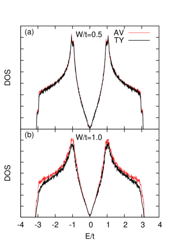
Figure 1: (Color online) Average (red) and typical (black) DOS for the lattice size $L=~{}80\times 10^{3}$ with $K_{r}\times K_{s}=15\times 15$ and $N=4000$ at disorder intensities (a) $W/t=~{}0.5$ and (b) $W/t=~{}1.0$

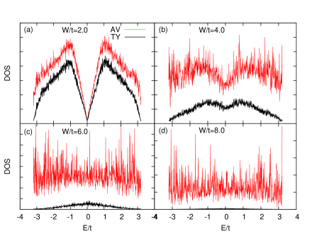
Figure 2: (Color online) Average (red) and typical (black) DOS for the lattice size $L=~{}80\times 10^{3}$ with $K_{r}\times K_{s}=15\times 15$ and $N=4000$ at disorder intensities (a) $W/t=~{}2.0$, (b) $W/t=~{}4.0$, (c) $W/t=~{}6.0$ and (d) $W/t=~{}8.0$.

Figure 3: (Color online) LDOS map for various disorder intensities for $E\in[0.0,0.01]$. In the weak disorder regime, the electron density is almost uniformly distributed over the entire lattice. By increasing $W/t$ to $8$, the electron density becomes confined in disconnected regions of lattice.

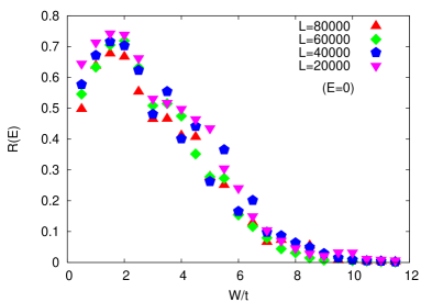
Figure 4: (Color online) The ratio of typical to average DOS ($R(E)$), computed at the band center ($E=0$), versus the strength of disorder for different lattice sizes $L=2\times 10^{4},4\times 10^{4},6\times 10^{4},8\times 10^{4}$.

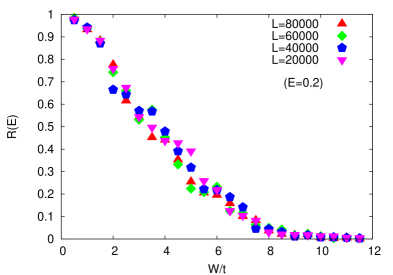
Figure 5: (Color online) The ratio of typical to average DOS ($R(E)$), computed at $E=0.2$ , versus the strength of disorder for different lattice sizes $L=2\times 10^{4},4\times 10^{4},6\times 10^{4},8\times 10^{4}$.

References

- (1) K. S. Novoselov, et al, Science 306, 666 (2004); K. S. Novoselov, et al, Nature (London) 438, 197 (2005).
- (2) A. H. Castro Neto, F. Guinea, N. M. R. Peres, K. S. Novoselov, A. K. Geim, Rev. Mod. Phys. 81, 109, (2009).
- (3) Y. Zhang, et al, Nature (London) 438, 201 (2005); Y. Zhang, et al, Phys. Rev. Lett. 96, 136806 (2006).
- (4) P. R. Wallace, Phys. Rev. 71, 622 (1947).
- (5) M. Y. Han et al, Phys. Rev. Lett. 98, 206805 (2007).
- (6) E. McCann and V. I. Fal’ko, Phys. Rev. Lett. 96, 086805 (2006).
- (7) E. McCann, Phys. Rev. B. 74, 161403 (2006); J. B. Oostinga, et al, Nature Mat. online 10.1038, nmat2082 (2007); E. V. Castro, et al, Phys. Rev. Lett. 99, 216802 (2007).
- (8) J. Nilsson, et al, Phys. Rev. B. 76, 165416 (2007).
- (9) J. Nilsson, A. H. Castro Neto, F. Guinea, N. M. R. Peres, phys. Rev. B 78, 045405 (2008).
- (10) C. Berger et al, J. Phys. Chem. B 108, 19912 (2004)
- (11) C. Berger et al, Science 312, 119:w 1 (2006)
- (12) J. Nilsson, A. H. Castro Neto, F. Guinea, N. M. R. Peres, Phys. Rev. Lett. 97, 266801 (2006).
- (13) K. S. Novoselov, E. McCacn, S. V. Morozov, V. I. Fal’ko, M. I. Katsnelson, U. Zeitler, D. Jiang, F. Schedin, A. K. Geim, Nature Phys. 2, 177 (2006).
- (14) Mikito Koshino and Tsuneya, Phys. Rev. B 73,245403 (2006).
- (15) E. Abrahams, P. W. Anderson, D. C. Licciardello, and T. V. Ramakrishnan, Phys. Rev. Lett. 42, 673 (1979).
- (16) E. Fradkin, Phys. Rev. B 63, 3263 (1986); P. A. Lee, Phys. Rev. Lett. 71, 1887 (1993); E. V. Gorbar, et al, Phys. Rev. B. 66, 045108 (2002); V. P. Gusynin, et al, Phys. Rev. Lett. 95, 24511 (2005); J. Csetri, Phys. Rev. B. 75, 033405 (2007).
- (17) I. Snyman, et al, Phys. Rev. B. 75, 045322 (2007).
- (18) M. Amini, S. A. Jafari, F. Shahbazi, Eur. Phys. Lett. 87, 37002 (2009).
- (19) Aaron Bostwick, Jessica L. McChesney, Konstantin V. Emtsev, Thomas Seyller, Karsten Horn, Stephen D. Kevan, and Eli Rotenberg, Phys. Rev. Lett. 103, 056404 (2009).
- (20) A. Weisse et al, Rev. Mod. Phys. 78, 275 (2006).
- (21) W. W. Toy, et al, Phys. Rev. B 15, 4077 (1977).
- (22) A. Misu, E. Mendez, M. S. Dresslhaus, J. Phys. Soc. Jpn 47, 199 (1979).
- (23) Lin-Wang Wang, Phys. Rev. B 49, 10154 (1994).
- (24) J. Stoer, and R. Bulirsch, Introduction to Numerical Analysis, Second Edn., Springer-Verlag, New York, 1993.
- (25) G. G. Naumis, Phys. Rev. B 76, 153403 (2007).
- (26) G. Schubert, et al, Phys. Rev. B 71, 045126 (2005).