The ACS LCID project. III. The star formation history of the Cetus dSph galaxy:
a post-reionization fossil.

Abstract

We use deep HST/ACS observations to calculate the star formation history (SFH) of the Cetus dwarf spheroidal (dSph) galaxy. Our photometry reaches below the oldest main sequence turn-offs, which allows us to estimate the age and duration of the main episode of star formation in Cetus. This is well approximated by a single episode that peaked roughly 12$\pm$0.5 Gyr ago and lasted no longer than about 1.9$\pm$0.5 Gyr (FWHM). Our solution also suggests that essentially no stars formed in Cetus during the past 8 Gyrs. This makes Cetus’ SFH comparable to that of the oldest Milky Way dSphs. Given the current isolation of Cetus in the outer fringes of the Local Group, this implies that Cetus is a clear outlier in the morphology-Galactocentric distance relation that holds for the majority of Milky Way dwarf satellites. Our results also show that Cetus continued forming stars through $z\simeq$ 1, long after the Universe was reionized, and that there is no clear signature of the epoch of reionization in Cetus’ SFH. We discuss briefly the implications of these results for dwarf galaxy evolution models. Finally, we present a comprehensive account of the data reduction and analysis strategy adopted for all galaxies targeted by the LCID (Local Cosmology from Isolated Dwarfs) project. We employ two different photometry codes (DAOPHOT/ALLFRAME and DOLPHOT), three different SFH reconstruction codes (IAC-pop/MinnIAC, MATCH, COLE), and two stellar evolution libraries (BaSTI and Padova/Girardi), allowing for a detailed assessment of the modeling and observational uncertainties.

1. Introduction

A powerful method to study the mechanisms that drive the evolution of stellar systems is the recovery of their full star formation history (SFH). This can be done by coupling deep and accurate photometry, reaching the oldest main sequence (MS) turn-off (TO), with the synthetic color-magnitude diagram (CMD) modeling technique (Tosi et al., 1991; Bertelli et al., 1992; Tolstoy & Saha, 1996; Aparicio et al., 1997; Harris & Zaritsky, 2001; Dolphin, 2002; Aparicio & Gallart, 2004; Cole et al., 2007; Aparicio & Hidalgo, 2009). The details of the first stages of galaxy evolution are particularly interesting, because they directly connect stellar populations research with cosmological studies. For example, the standard paradigm predicts that the role of re-ionization can impact the star formation history of small systems in a measurable way (e.g., Ikeuchi, 1986; Rees, 1986; Efstathiou, 1992; Babul & Rees, 1992; Chiba & Nath, 1994; Quinn, Katz, & Efstathiou, 1996; Thoul & Weinberg, 1996; Kepner, Babul, & Spergel, 1997; Barkana & Loeb, 1999; Bullock et al., 2000; Tassis et al., 2003; Ricotti & Gnedin, 2005; Gnedin & Kravtsov, 2006; Okamoto & Frenk, 2009).

In this context, we designed a project aimed at recovering the full SFHs of six isolated galaxies in the Local Group (LG), namely IC 1613, Leo A, LGS 3, Phoenix, Cetus, and Tucana, with particular focus on the details of the early SFH. Isolated systems were selected because they are thought to have completed few, if any, orbits inside the LG. Therefore, compared to satellite dSphs, they spent most of their lifetime unperturbed, so that their evolution is expected not to be strongly affected by giant galaxies. A general summary of the goals, design and outcome of the LCID project can be found in Gallart et al. (in prep), where a comparative study of the results for the six galaxies is presented.

In this paper we focus on the stellar populations of the Cetus dSph galaxy only. This galaxy was discovered by Whiting et al. (1999), by visual inspection of the ESO/SRC plates. From follow-up CCD observations they obtained a CMD to a depth of $V\sim 23$, clearly showing the upper part of the red giant branch (RGB), but no evidence of a young main sequence, nor of either red or blue supergiants typical of evolved young populations. From the tip of the RGB (TRGB) they could estimate a distance modulus $(m-M)_{0}=24.45\pm 0.15$ mag ($776\pm 53$ kpc), assuming $E(B-V)=0.03$ from the Schlegel et al. (1998) maps and an absolute magnitude $M_{I}(TRGB)=-3.98\pm 0.05$ mag for the tip. The color of the RGB stars near the tip allowed a mean metallicity estimate of $[Fe/H]=-1.7$ dex with a spread of $\sim 0.2$ dex. Deeper HST/WFPC2 data presented by Sarajedini et al. (2002) confirmed the distance modulus of Cetus: $(m-M)_{0}=24.49\pm 0.14$ mag, or $790\pm 50$ kpc, assuming $M_{I}(TRGB)=-4.05\pm 0.10$ mag. Based on the color distribution of bright RGB stars, they estimated a mean metallicity $[Fe/H]=-1.9$ dex. An interesting feature of the Cetus CMD presented by Sarajedini et al. (2002) is that the horizontal branch (HB) seems to be more populated in the red than in the blue part (see also the CMD by Tolstoy et al., 2000, based on VLT/FORS1 data). Sarajedini et al. (2002) calculated an HB $index=-0.91\pm 0.09$. By using an empirical relation between the mean color of the HB and its morphological type, derived from globular clusters of metallicity similar to that of Cetus, they concluded that the Cetus HB is too red for its metallicity, and therefore, is to some extent affected by the so-called second parameter. Assuming that this is mostly due to age, they proposed that Cetus could be 2-3 Gyr younger than the old Galactic globular clusters.

Recent work by Lewis et al. (2007) presented wide-field photometry from the Isaac Newton Telescope together with Keck spectroscopic data for the brightest RGB stars. From CaT measurements of 70 stars, they estimated a mean metallicity of $[Fe/H]=-1.9$ dex, fully consistent with previous estimates based on photometric data. Moreover, they determined for the first time a systemic heliocentric velocity of $\sim$ 87 km s^-1, an internal velocity dispersion of 17 km s^-1 and, interestingly enough, little evidence of rotation.

The search for H I gas (Bouchard et al., 2006) revelead three possible candidate clouds associated with Cetus, located beyond its tidal radius, but within 20 Kpc from its centre. Considering the velocity of these clouds, Bouchard et al. (2006) suggested that the velocity of Cetus should be of the order of -280$\pm 40km~{}s^{-1}$ to have a high chance of association. Clearly, this does not agree with the estimates later given by Lewis et al. (2007), who pointed out that Cetus is devoid of gas, at least to the actual observational limits.

Cetus is particularly interesting for two distinctive characteristics. First, the high degree of isolation, it being at least $\sim 680$ kpc away from both the Galaxy and M31. Cetus is, together with Tucana, one of the two isolated dwarf spheroidals in the LG. Moreover, based on wide-field INT telescope data, McConnachie & Irwin (2006) estimated a tidal radius of 6.6 kpc, which would make Cetus the largest dSph in the LG. Therefore, an in-depth study of its stellar populations, and how they evolved with time, could provide important clues about the processes governing dwarf galaxy evolution.

The paper is organized as follows. In §2 we present the data and the reduction strategy. §3 discusses the details of the derived color-magnitude diagram (CMD). In §4 we summarize the methods adopted to recover the SFH, and we discuss the effect of the photometry/library/code on the derived SFH. The Cetus SFH is presented in §5, where we discuss the details of the results, as well as the tests we performed to estimate the duration of the main peak of star formation and the radial gradients. A discussion of these results in the general context of galaxy evolution are presented in §6, and our conclusions are summarized in §7.

2. Observations and data reduction strategy

The data presented in this paper were collected with the ACS/WFC camera (Ford et al., 1998) aboard the HST. The observations were designed to obtain a signal-to-noise ratio $\approx 10$ at the magnitude level of the oldest MSTO, $M_{F814W}\sim+3$. Following the precepts outlined in Stetson (1993), the choice of the filters was based on the analysis of synthetic CMDs in the ACS bands. The $(F475W-F814W)$ pair, due to the large color baseline together with the large filter widths, turned out to be optimal for separating age differences of the order of 1-2 Gyr in stellar populations older than 10 Gyr.

The observations were split into two-orbit visits. One $F475W$ and one $F814W$ image were collected during each orbit, with exposure times slightly different between the two orbits of the same visit: 1,280 s and 1,135 s, respectively, in the first orbit, 1,300 s and 1,137 s during the second one. The last visit included a third orbit, with exposure times of 1,300 s and 1,137 s. The 27 orbits allocated to this galaxy were executed between August 28 and 30, 2006. The two orbits corresponding to the ninth visit (images j9fz27glq, j9fz27gmq, j9fz27goq, j9fz27gqq) suffered from loss of the guide star. Therefore, two images were found to be shifted by $\approx$1.5$\arcmin$, and the other two were aborted after a few seconds. These data will not be included in the following analysis. Summarizing, the total exposure time devoted to Cetus and used in this work was 32,280 s in $F475W$ and 28,381 s in $F814W$.

For our observing strategy, we split each orbit into one $F475W$ and one $F814W$ exposure in order to have the best possible time sampling for short-period variable stars (see Bernard et al., 2009). An off-center pointing was chosen to sample a wide range of galactocentric radii. The edge of the ACS camera was shifted to the south by $\sim 2\arcmin$ from the center of Cetus, in order to avoid a bright field star. The coordinates of the ACS pointings are [$RA=00^{h}26^{m}09^{s}.70,DEC=-11\arcdeg 04\arcmin 34.7\arcsec$]. Fig. 1 shows the location of both the ACS and the parallel WFPC2 field [$RA=00^{h}25^{m}51^{s}.41,DEC=-11^{\circ}00\arcmin 32.4\arcsec$]. The pointing of the latter was optimized to explore the outskirts of the galaxy, and the resulting CMD has already been presented in Bernard et al. (2009). Due to the much shallower photometry in the WFPC2 field, this will not be included in the analysis of the SFH. Fig. 2 shows a color drizzled, stacked image. Note the strong gradient in the number of stars when moving outward toward the south. There are also a few bright field stars, and a sizable number of extended background sources.

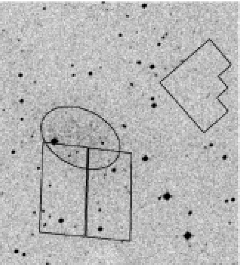
Figure 1.— 9$\arcmin\times$ 9$\arcmin$ DSS image showing the ACS and the WFPC2 pointings. The ellipse represents the Cetus core radius.

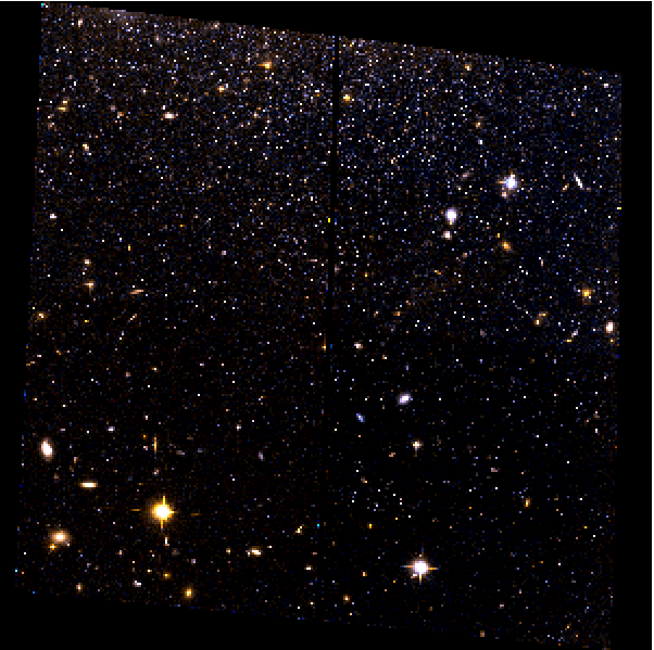
Figure 2.— Stacked, drizzled color image of the Cetus field. North is up and East is left. The field of view is $\sim$3.4$\times$3.4 square arcmin. The image shows a clear gradient in the number of stars when moving toward the south. Note the considerable number of background galaxies.

In the following, we outline the homogeneous reduction strategy adopted for all the galaxies of the LCID project. In particular, we stress that we performed two parallel and independent photometric reductions, based on the DAOPHOT/ALLFRAME (Stetson, 1994) and the DOLPHOT packages (Dolphin, 2000b), in order to investigate the impact of using different photometry codes to obtain the CMD used to derive the SFH (see §4.4).

2.1. DAOPHOT reduction

After testing different approaches to drizzle the set of images, we opted to work on the original _FLT data. A custom dithering pattern was adopted for the observations. The shifts applied were small enough ($<10$ pixels) that the camera distortions would not cause problems when subsequently merging the catalogs from different images. The two chips of the camera have been treated independently, and we applied the following steps to all the individual images:

$\bullet$ Basic reduction: we adopted the basic reduction (bias, flat field) from the On-The-Fly-Reprocessing pipeline (CALACS v.4.6.1, March 13 2006). Since we opted for the _FLT images, we applied the pixel area mask to account for the different area of the sky projected onto each pixel, depending on its position;

$\bullet$ Cosmic ray rejection: we used the data quality files from the pipeline to mask the cosmic rays (CR). According to the flag definition in the ACS Data handbook, pixels with the value 4096 are affected by cosmic rays. These pixels were flagged with a value higher than the saturation threshold. This allowed DAOPHOT to recognize and properly ignore them;

$\bullet$ Aperture photometry: we performed the source detection at a 3-$\sigma$ level and aperture photometry, with aperture radius=3 pixels;

$\bullet$ PSF modeling: careful selection of the PSF stars was done through an iterative procedure. Automated routines were used to identify bright, isolated stars, with good shape parameters (sharpness) and small photometric errors. PSF stars were selected in order to sample the whole area of the chip, to properly take into account the spatial variations of the PSF. The last step was a visual inspection of all the PSF stars, for all the images, to reject those with peculiarities like bright neighbors, contamination by CRs, or damaged columns. On average, we ended up with more than 150 PSF stars per image.

We performed many tests in order to understand which PSF model, among those available in DAOPHOT, would work best with our data. We used the same sets of stars for each fixed analytical PSF model, and tested different degrees of variation across the field, from purely analytical and constant ($variability=-1,0$) to varying cubically ($va=3$). We evaluated the quality of the final CMD, and the best results were obtained with $va>0$, but the tightness of the CMD sequences did not vary appreciably when using a quadratically or cubically variable PSF. We also checked the photometric errors and sharpness estimators, but could not find any evident improvement when increasing the degree of variation of the PSF. We therefore adopted a simpler and faster linear PSF, allowing the software to choose the analytical function on the basis of the $\chi^{2}$ estimated by the $PSF$ routine. In all the images, a Moffat function with index $\beta$ = 1.5 was selected.

The next step was ALLSTAR profile-fitting photometry for individual images. The resulting catalogs were used only to calculate the geometric transformations with respect to a common coordinate system, using DAOMATCH and DAOMASTER. Geometrical transformations are needed to generate a stacked image with MONTAGE2. The resulting median CR-cleaned image was used to create the input list for ALLFRAME. Rejecting all the objects with $|sharp|>0.3$ was an efficient way to remove most of the extended objects (i.e., background galaxies), as well as remaining cosmic rays. After the first ALLFRAME was run, we used the updated and more precise positions and magnitudes to refine the coordinate transformations and to recalculate the PSFs, using the previously selected list of stars. A second ALLFRAME run was finally ran with updated geometric transformations and PSFs.

The calibration to the VEGAMAG system was done following the prescriptions given by Sirianni et al. (2005), using the updated zero points from Mack et al. (2007) (because Cetus was observed after the temperature change of the camera in July 2006). Particular attention was paid to calculate the aperture correction to the default aperture radius of 0.5″. Aperture photometry in various apertures was performed on the PSF stars of every image, once the neighboring stars had been subtracted. The growth curve and total magnitude of the stars were obtained using DAOGROW (Stetson, 1990). An aperture correction was calculated for every image, with the result that the mean correction was 0.029 $\pm$ 0.009 mag. Individual catalogs were calibrated, and the final list of stars was obtained keeping all the objects present in at least (half+1) images in both bands. The final CMD is presented and discussed in §3.

2.2. Crowding tests with DAOPHOT

To estimate the completeness and errors affecting our photometry, we adopted a standard method of artificial-star tests. We added $\sim$ 350,000 stars per chip, adopting a regular grid where the stars were located at the vertices of equilateral triangles. The distance between two artificial stars was fixed in order to pack the largest number of stars but at the same time to ensure that the synthetic stars were not affecting each other. This value was chosen to be R = ($rad_{PSF}$ + $rad_{fit}$ + 1) = 13 pixels. In this way, overlapping of the wings of the artificial stars was minimized to avoid influencing the fit in the core of the PSF. With this criterion, taking into account the dimension of the CCD, we needed seven iterations with $\sim$ 49,770 stars each. In each iteration, the grid was moved by a few pixels, to better sample the crowding characteristics of the image.

To verify the hypothesis that the synthetic stars were not affecting each other, we also performed completeness tests injecting stars separated by ($2\times rad_{PSF}$ + 1) = 21 pixels. We did not find any significant difference in the completeness level of synthetic stars, meaning that the original separation was adequate. With this criterion, the incompleteness of the synthetic stars only depends on the real stars, while the additional crowding due to the partial overlap of the injected stars is negligible.

The list of injected stars was selected following the prescriptions introduced by Gallart et al. (1996). To fully sample the observed magnitude and color ranges, we adopted a synthetic CMD created with IAC-star (Aparicio & Gallart, 2004), adopting a constant star formation rate (SFR) between 0 and 15 Gyr, with the metallicity uniformly distributed between Z=0.0001 and Z=0.005 at any age. The stars were added on the individual images, taking into account the coordinate and magnitude shifts. The photometry was then repeated with the same prescriptions as for the original images. The results are summarized in Fig. 3, where the $\Delta mag$=mag_in-mag_out of the artificial stars and selected completeness levels are shown for the two bands, as a function of the input magnitude.

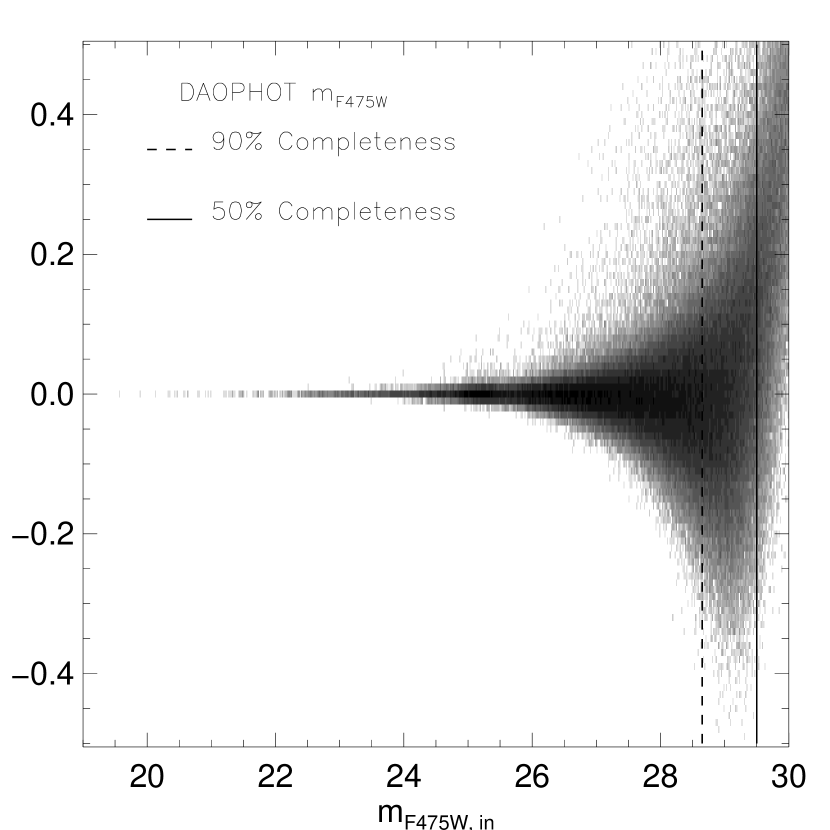
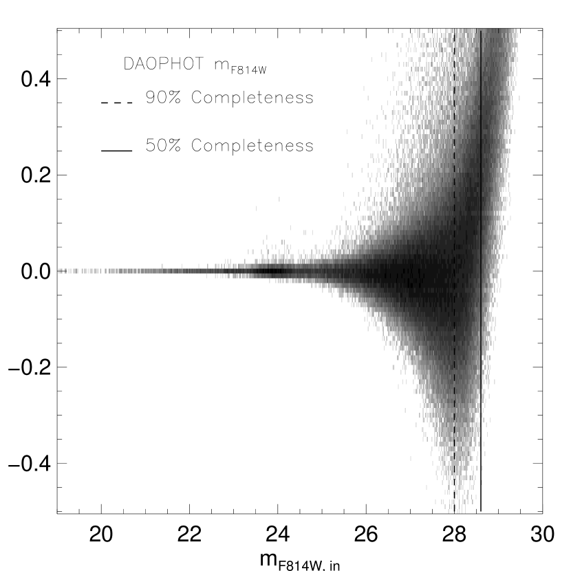
Figure 3.— Difference $\Delta mag$=mag_in-mag_out for synthetic stars. The two vertical lines mark the 90% and 50% completeness level. A total of $\sim$700,000 stars were simulated.

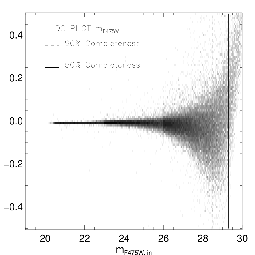
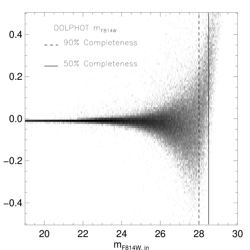
Figure 4.— Same as Fig. 3, but for the DOLPHOT photometry. A total of $\sim$140,000 stars were simulated.

2.3. DOLPHOT reduction

DOLPHOT is a general-purpose photometry package adapted from the WFPC2-specific package HSTphot (Dolphin, 2000b). For this reduction, we used the ACS module of DOLPHOT and followed the recommended photometry recipe provided in the manual for version 1.0.3. The procedure is fairly automated, with the software locating stars, adjusting the default Tiny Tim PSFs based on the image, iterating until the photometry converges, and making aperture corrections. Similar to the procedures with DAOPHOT, we used the original _FLT images, corrected for the pixel-area mask and cosmic rays. We used a drizzled image from the HST archive as the reference for the coordinate transformations. The search for stellar sources was performed with a threshold $t$=2.5$\sigma$. The photometry was done fitting a model PSF calculated with TinyTim. DOLPHOT also automatically estimated the aperture correction to 0.5$\arcsec$. The same calibration as for the DAOPHOT photometry was used.

2.4. Crowding tests with DOLPHOT

Artificial-star tests were preformed by injecting $\sim 140,000$ synthetic stars in the original images. The input colors and magnitudes of the synthetic stars cover the complete range of the observed colors and magnitudes. The stars uniformly sample the range $-1<M_{F475W}-M_{814W}<5$ mag, $-7<M_{F475W}<8$ mag. The photometry was performed following the procedure suggested by Holtzman et al. (2006). The synthetic stars were injected one at a time into the images to avoid affecting the stellar crowding in the images. Stars were uniformly distributed to cover the whole area of the camera. Fig. 4 shows $\Delta mag$=mag_in-mag_out of the artificial stars together with the 50% and 90% completeness levels for the two bands.

2.5. Comparison of the two photometry sets

A direct comparison between the DAOPHOT and DOLPHOT photometry is presented in Fig. 5. We detect a small zero point offset for the brightest stars in both bands ($(m_{F475W,DAO}-m_{F475W,DOL})\sim 0.023$ mag, for $m_{F475W}<$ 25, and $(m_{F814W,DAO}-m_{F814W,DOL})\sim-0.010$ mag, for $m_{F814W}<$ 24), and a trend as a function of magnitude: moving toward fainter magnitudes, DAOPHOT tends to give slightly fainter results (up to $\Delta m_{F475W}\simeq$ 0.05 mag, at $m_{F475W}=29.1$, $\Delta m_{F814W}\simeq 0.07$ at $m_{F814W}=28.0$). Note that since the trend with magnitude is similar in the two bands, the color difference shows a residual zero point offset ($\sim 0.04$ mag), but no dependence on magnitude. We performed an exhaustive search for the possible cause of such small differences, but its origin remained elusive, and it is likely a result of the many differences between the approaches of the two photometric packages (PSF, sky determination, aperture correction calculation). Note that similar trends were detected and discussed by Holtzman et al. (2006) and Hill et al. (1998) when comparing different photometric codes applied to HST data. This reinforces the idea that small differences in the resulting photometry naturally arise when using different reduction codes, at least when dealing with HST data.

However, we highlight that, for this project, the MinnIAC/IAC-pop method presented in 4.1 is not sensitive to zero-point systematics, and therefore the impact of small differences in the photometry on the derived SFH is minimized.

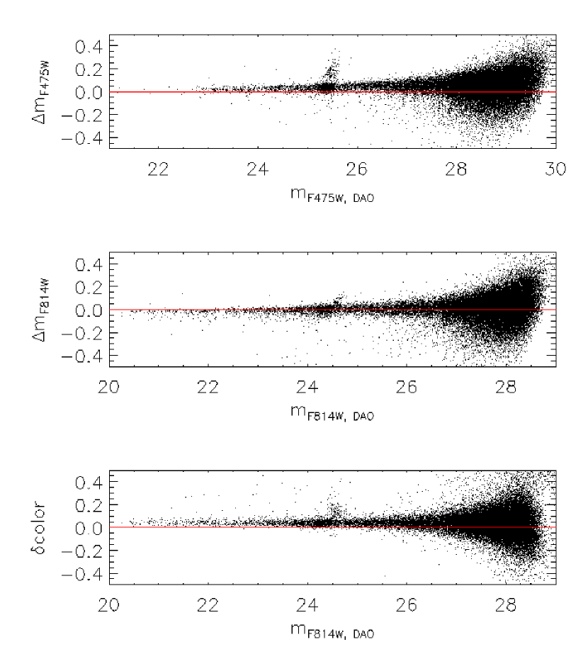
Figure 5.— Magnitude and color difference between the DAOPHOT and DOLPHOT photometry, as a function of the DAOPHOT magnitude. We detect a systematic residual zero point between the two codes, and a small trend as a function of magnitude. At the faintest end, DAOPHOT gives fainter measurements than DOLPHOT. However, since the trend is similar in the two filters, the color difference showed only a small residual zero point of the order of 0.04 mag. The plume of objects at $m_{F475W}\sim 25.5$ is made of RR Lyrae variable stars.

3. The color-magnitude diagram

Fig. 6 presents the final CMD from both the DAOPHOT and DOLPHOT photometry, calibrated to the VEGAMAG system. This is the deepest CMD obtained to date for this galaxy, spanning more than 8 mag, from the TRGB down to $\approx$1.5 mag below the oldest MSTO. The limiting magnitude (F814W $\sim$ 28.8 mag) is similar in both diagrams. No selections were applied to the DAOPHOT CMD other than those already applied to the star list, while the DOLPHOT photometry was cleaned according to the sharpness ($|sharp|<0.1$), crowding ($crowd<0.7$), and photometric errors ($\sigma_{m_{F475W}},\sigma_{m_{F814W}}<0.2$). The DAOPHOT and DOLPHOT CMDs contain $\sim$ 50,600 and 44,900 stars, respectively

A simple qualitative analysis reveals many interesting features. The TO emerges, for the first time and very well characterized in our photometry, at $m_{F814W}\sim$ 27 mag. The morphologies of the TO and the sub-giant branch region suggest that Cetus is a predominantly old system. There is no evidence of bright main sequence stars indicative of recent star formation. A plume of relatively faint objects appears at 26 $<m_{F814W}<$ 28, 0 $<(m_{F475W}-m_{F814W})<$ 0.5, and could indicate either a low level of star formation until $\sim$ 2-3 Gyr ago, or the presence of a population of blue straggler stars (BSs) (cf., Mapelli et al., 2007; Momany et al., 2007; Mapelli et al., 2009). We noticed that the over-density right above the TO, at $0.8<(m_{F475W}-m_{F814W})<1,26.5<m_{F814W}<27.0$, is mostly present in the central regions. We verified that, with the DAOPHOT photometry, such overdensity appears as well in the CMD of the synthetic stars used in the completenss tests and located in the most crowded areas of the images. Since we simulated the same CMD in all the regions of the camera, there is no reason to expect differences in the output synthetic CMDs as a function of the position. This indicates that the higher crowding in the central region is responsible for this feature. Nevertheless, it is possible that some of the stars located in this region are physical binaries.

Concerning the evolved phases of stellar evolution, the RGB between 20 $<m_{F814W}<$ 26.5 mag appears as a prominent feature. The width of the RGB is similar in both diagrams, and suggests some spread in age and/or metallicity. The sudden increase in the RGB width at $m_{F814W}\leq$ 23.2 may be explained by the superposition of the RGB and the asymptotic giant branch (observational effects like saturation of bright stars or loss of linearity of the camera can be safely excluded in this regime).

The HB, as already noted by Sarajedini et al. (2002) and Tolstoy et al. (2000) is dominated by stars redder than the RR Lyrae instability strip. However, even if sparsely populated, a blue HB emerges clearly from our photometry. It is difficult to estimate how extended it is on the blue side, because it merges with the sequence of blue candidate MS stars/BSs. We also note that there are a small number of objects on both the blue ($m_{F814W}<$ 23 mag, $(m_{F475W}-m_{F814W})\sim$ 1) and red side of the RGB. These are most likely foreground field stars.

We can gain some insight into the Cetus stellar populations through a comparison with theoretical isochrones, which allows us to estimate some rough limits to the ages and metallicities of the stellar populations. Fig. 7 presents the superposition of selected isochrones from the BaSTI database (Pietrinferni et al., 2004), for the indicated ages and metallicities. For simplicity, we adopted the DAOPHOT photometry, but the conclusions are independent of the photometry set. The distance, $(m-M)_{0}=24.49$, was estimated using the mean magnitude of the RR Lyrae stars (Bernard et al., 2009). An attempt to use the TRGB showed that the number of stars near the tip is too small to derive a precise estimate of the distance modulus. However, the excellent agreement between the TRGB of the isochrones with the brightest stars of the RGB in Fig. 7 shows that this distance is very reliable. The extinction $E(B-V)=0.03$ was taken from Schlegel et al. (1998), and was transformed to A_F475W and A_F814W following Bedin et al. (2005).

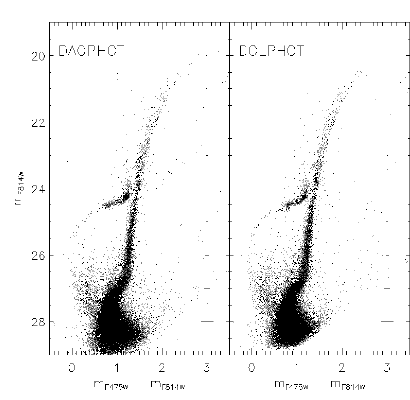
Figure 6.— Color-magnitude diagram, calibrated in the VEGAMAG photometric system, for both the DAOPHOT and DOLPHOT photometry. On the right side of both panels we report the mean magnitude and color fitting errors provided by the two codes.

The left panel of Fig. 7 shows the comparison with young isochrones. The blue edge of the blue plume can be well matched with a metal-poor (Z = 0.0001), relatively young (2 Gyr) isochrone (red line). A similarly good agreement with isochrones of higher metallicity (Z = 0.001, 0.002, green and blue lines) is obtained only by reducing the age considerably (0.5 Gyr), but the lack of observed bright TO stars makes this interpretation unlikely. An increase in the age for the Z = 0.001 isochrone (pink line) cannot account for the observationally well measured blue portion of this feature. This might suggest that this is a sequence of BSs rather than a truly young MS (see also §5.2.1).

The right panel of the same figure shows the comparison with isochrones of age ranging from 7 to 14 Gyr, and metallicities Z = 0.0001 and Z = 0.001. It is interesting to note that both the TO and RGB phases are well confined in this metallicity range. In particular, the blue edge of the RGB seems to correspond to the lower metallicity, while the red edge is well constrained by a metallicity 10 times higher, with negligible dependence on age. The situation around the TO is more complicated. At fixed metallicity, the oldest isochrone matches the faint red edge of the TO reasonably well, while the youngest nicely delimits the brighter and bluer one. Therefore, both the faint red and the bright blue edges can be properly represented using either an older, more metal-poor, or a slightly younger, more metal-rich isochrone.

However, from this simple analysis, we can not set strong constraints. A possible interpretation is that Cetus consists of a dominant population of age 10 Gyr, with a small age range and with metallicity in the range 0.0001 $<$ Z $<$ 0.001. Alternatively, and equally consistent with this simple analysis, is a scenario with both age and metallicity spreads. Therefore, this simplistic analysis is only helpful to put loose constraints on the expected populations, in terms of ages and metallicities, but does not allow us to draw any quantitative conclusions on the age and metallicity distribution of the observed stars. For that, a more sophisticated analysis is required such as the one presented in §4 below.

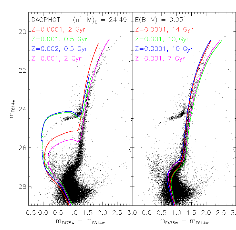
Figure 7.— Color-magnitude diagram, calibrated in the VEGAMAG photometric system, with overimposed some selected isochrones from the BaSTI database, shifted according to the labeled distance modulus and reddening values. Age and metallicity of the isochrones are also labeled in the figure.

3.1. The RGB bump

The RGB bump is a feature commonly observed in old stellar systems (e.g., Riello et al., 2003), whose physical origin is relatively well understood (Thomas, 1967; Iben, 1968). When a low-mass star ascends the RGB, the H-burning shell moves outward and reaches the chemical discontinuity left by the convective envelope at the time of its greatest depth. This forces a rearrangement of the stellar structure and a temporary decrease in luminosity, before the star resumes evolving toward higher luminosities and lower effective temperatures. From the observational point of view, since the star crosses the same luminosity interval three times, it produces an accumulation of objects at one point in the luminosity function of the RGB. Fig. 8 shows the observed Cetus RGB luminosity function for both sets of photometry. The sample stars were selected in a box closely enclosing the RGB, in order to minimize the contribution of AGB and HB stars. The RGB bump clearly shows up, and fitting a Gaussian profile indicates a peak magnitude of $m_{F814}\sim$ 23.84 $\pm 0.08$, with excellent agreement between the two photometry sets.

Figure 8.— Luminosity function of the Cetus RGB, for both the DAOPHOT (solid line) and DOLPHOT (dashed) photometry. The vertical line shows the position of the RGB bump.

4. Derivation of the star formation history of Cetus

In this section we present the various approaches used to derive the SFH of Cetus. In particular, we adopted the two sets of photometry previously described, two stellar evolution libraries, BaSTI (Pietrinferni et al., 2004) and Padova/Girardi (Girardi et al., 2000; Marigo et al., 2008), and three different SFH codes: IAC-pop (Aparicio & Hidalgo, 2009), MATCH (Dolphin, 2002), and COLE (Skillman et al., 2003). We did not explore all the possible combinations of photometry/library/method, but we derived different solutions useful for comparison purposes, and to search for possible systematics. In particular, IAC-pop was applied to both sets of photometry and libraries, while MATCH and COLE were tested with the DOLPHOT photometry in combination with the Girardi library.

4.1. The IAC method

This method has been developed in recent years by members of the Instituto de Astrofísica de Canarias (A.A., S.H., C.G.), and now includes different independent modules. Each software package has been presented in different papers (IAC-star: Aparicio & Gallart 2004, MinnIAC: Hidalgo et al., in prep., IAC-pop: Aparicio & Hidalgo 2009), which are the reference publications for the interested reader and include appropriate references. In the following we give only a practical overview of the parameters adopted to derive the SFH of Cetus.

The entire procedure can be divided into five steps. Note that in the following we will use “synthetic CMD” to designate the CMD generated with IAC-star, and we will call it a “model CMD” if the observational errors have been simulated in the synthetic CMD.

1) The synthetic CMD: it is created using IAC-star (Aparicio & Gallart, 2004). We calculated a synthetic CMD with 8,000,000 stars from the inputs described in the following. We have verified that, with this large number of stars, no systematic effects in the derived SFH of mock galaxies—such as those discussed in Nöel et al. (2009)—were observed, and so no corrections such as those described in that paper are necessary. The requested inputs are:

• a set of theoretical stellar evolution models. We adopted the BaSTI (Pietrinferni et al., 2004) and Padova/Girardi (Girardi et al., 2000) libraries;

• a set of bolometric corrections to transform the theoretical stellar evolution tracks into the ACS camera photometric system. We applied the same set, taken from Bedin et al. (2005), to both libraries.

• the SFR as a function of time, $\psi(t)$. We used a constant SFR in the age range $0<t<15$ Gyr;

• No a priori age-metallicity relation Z(t) is adopted: the stars of any age have metallicities uniformly distributed in the range 0.0001$<$ Z $<$0.005. We stress that the age and metallicity intervals are deliberately selected to be wider than the ranges expected in the solution. This is done to ensure that no information is lost, and to provide the code with enough degrees of freedom to find the best possible solution;

• the initial mass function (IMF), taken from Kroupa (2002). This is expressed with the formula $N(m)~{}dm=m^{-\alpha}~{}dm$, where $\alpha$ = 1.3 for stars with mass smaller than 0.5 M_⊙, and $\alpha$ = 2.3 for stars of higher mass. Different values of both exponents have been tested with IC 1613 and LGS 3. The results, presented in Skillman et al. (in prep.), show that the best solutions are obtained with values compatible with the Kroupa IMF;

• the binary fraction, $\beta$, and the relative mass distribution of binary stars, $q$ . We tested six values of the binary fraction, from 0% to 100%, in steps of 20%, with fixed $q>$ 0.5; in the following analysis we use 40% and discuss the impact of different assumptions in the Appendix I;

• the assumed mass loss during the RGB phase follows the empirical relation by Reimers (1975), with efficiency $\eta=0.35$.

2) The error simulation: The code to simulate the observational errors in the synthetic CMD, called obsersin, has been developed following Gallart et al. (1996), and is described in Hidalgo et al., in prep. It takes into account the incompleteness and photometric errors due to crowding using an empirical approach, taking the information from the completeness test described in §2.2 and §2.4. This is a fundamental step because the distribution of stars in the observed CMD is strongly modified from the actual distribution due to the observational errors, particularly at the faint magnitude level near the old TO, which is where most of the information on the most ancient star formation is encoded. Fig. 9 shows an example of synthetic CMD as generated by IAC-star (upper panel), and after the dispersion according to the observational errors of Cetus (lower panel).

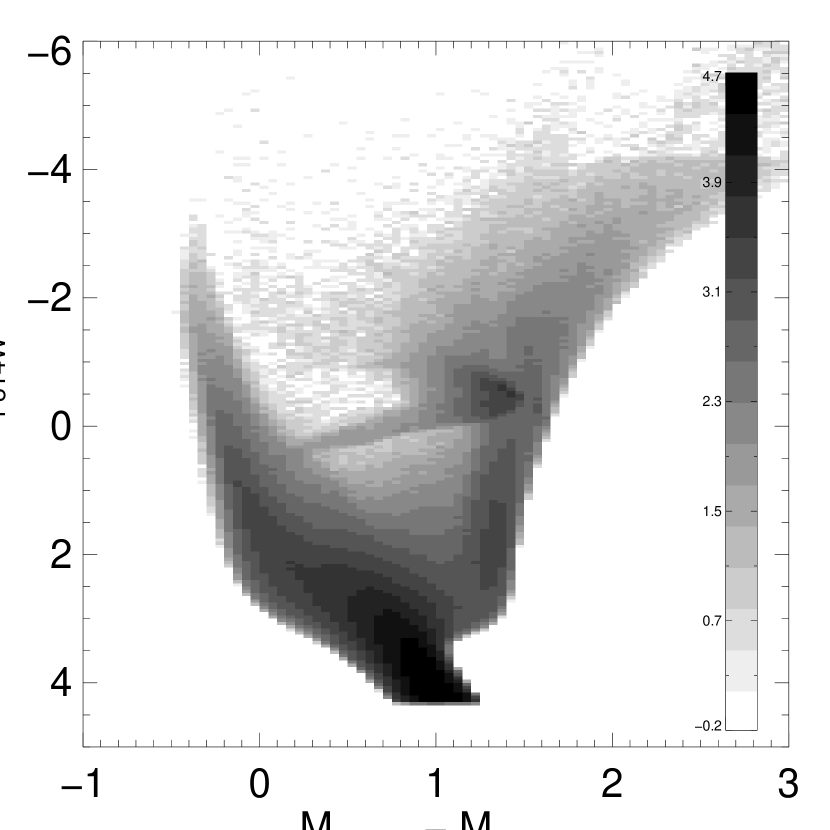
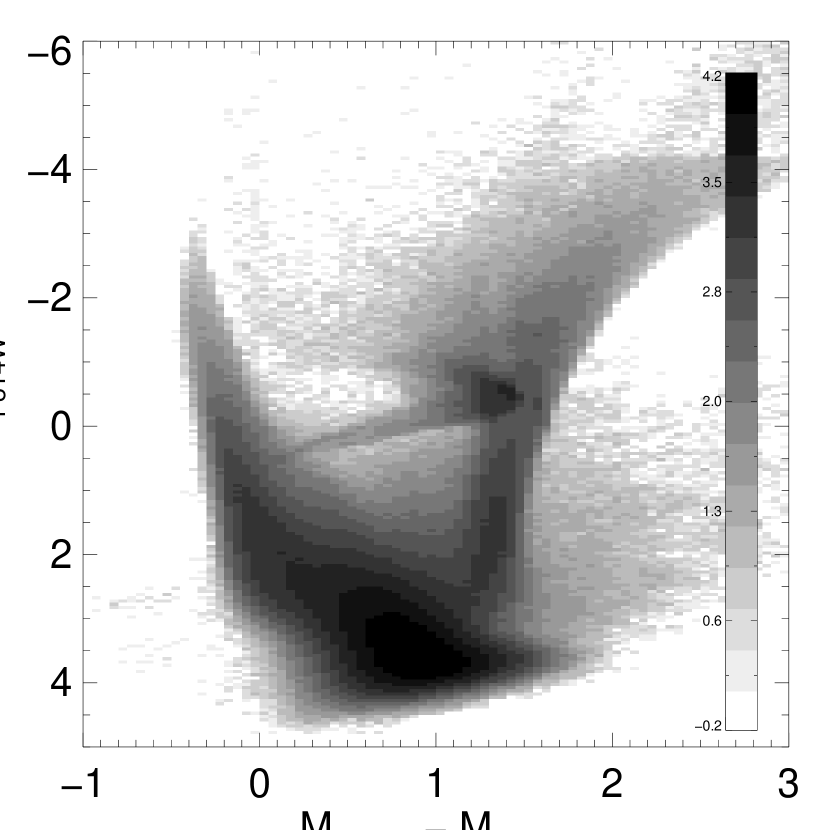
Figure 9.— Hess diagram of the 8 $\times 10^{6}$ stars synthetic CMD generated with IAC-star (upper) and after simulating the observational errors (lower).

3) Parameterization: MinnIAC is a suite of routines developed specifically to accomplish two main purposes: first, an efficient sampling of the parameter space to obtain a set of solutions with different parametrizations of the CMD, and second, estimation of the average SFH from the different solutions that best represent the observations. In our case, “parameterization” of the CMD means two things: i) defining the age and metallicity bins that fix the simple populations and ii) defining a grid of boxes covering critical evolutionary phases in the CMDs, where the stars of the observed and model CMD are counted.

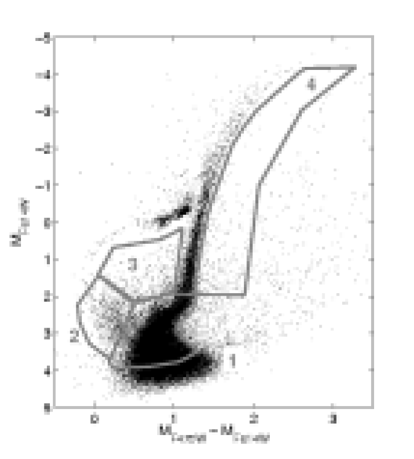
Figure 10.— Cetus observed CMD, transformed to the absolute plane assuming (m-M)₀ = 24.49 and E(B$-$V)=0.03, with the location of the four bundles superimposed.

The basic age and metallicity bins defining the simple populations used in this work are:
age : [1.5 2 3 … 13 14 (15)]*10⁹ years
metallicity : [0.1 0.3 0.5 0.7 1.0 1.5 2.0]*10^-3

Note that model stars younger than 1.5 Gyrwere not included because there is no evidence of their presence in Cetus. These numbers define the boundaries of the bins, not their centers. Therefore, they fix $15\times 6=90$ simple populations. The choice of a 1 Gyr bin size at all ages was adopted after testing a range of bin widths. It was found that smaller bins do not increase the age resolution; rather they increase the noise in the solution. The selected size of 1 Gyr is the optimal compromise to fully exploit the data, within the limits imposed by the observational errors and the intrinsic age resolution in the CMD at old ages.

The parameterization of the CMD relies on the concept of bundles (see Aparicio & Hidalgo 2009 and Fig. 10), that is, macro-regions on the CMD that can be sub-divided into boxes using different appropriate samplings. The number of boxes in the bundle determines the weight that the region has for the derived SFH. This is an efficient and flexible approach for two reasons. First, it allows a finer sampling in those regions of the CMD where the models are less affected by the uncertainties in the input physics (MS, SGB). Second, the dimensions of the boxes can be increased, and the impact on the solution decreased, in those regions where the small number of observed stars could introduce noise due to small number statistics or where we are less confident in the stellar evolution predictions. We optimized the values for this work using four bundles, with the following box sizes. The smallest boxes ($0.01~{}mag\times 0.2~{}mag$, N1 $\sim$ 900 boxes) sample the lower (old) MS, and the SGB (bundle 1). The region of the candidate BSs (bundle 2) is mapped with slightly bigger boxes ($0.03~{}mag\times 0.5~{}mag$, N2 $\sim$ 90 boxes), to minimize the number of boxes with zero or few stars. Bundle 3 samples the region between the BS sequence and the RGB. No bundles include the stars in evolved evolutionary phases, and in particular we excluded both the RGB and the HB from our analysis. The reasons are many. First, the physics governing these evolutionary phases is more uncertain than that describing the MS, and differences between stellar libraries are more important in these evolved phases (Gallart et al., 2005). Moreover, the details of the HB morphology also depend on highly unknown factors like the mass loss during the RGB phase. However, despite not including the RGB stars, we routinely adopt a bundle which is redder than the RGB (bundle 4 in Fig. 10). In order to aid in setting a mild constraint on the upper limit of the metallicity of the RGB Cetus stars, this was drawn at the red edge of the RGB. It includes metal rich stars present in the model, but very few objects of the observed CMD. Both bundles 3 and 4 contain boxes of $1.5~{}mag\times 1.0~{}mag$ (N3 = 7, N4 = 4). Extensive tests have shown that including a bundle on the RGB did not improve the solution, nor produce a solution significantly different. Rather, the $\chi^{2}$ of the solution increases substantially and likely spurious populations appear in the 3D histogram, such as old and metal-rich stars.

For a given set of input parameters, the simple populations plus the grid of bundles+boxes, MinnIAC counts the stars in the boxes for both the observed and all the simple populations in the model CMD. A simple table with these star counts is the input information to run IAC-pop. However, our numerous tests disclosed that this approach can be significantly improved by adopting a series of slightly different sets of input parameters, used to derive many solutions and then calculating the mean SFH. This “dithering approach”, which is the distinctive feature of the code, significantly reduces the fluctuations associated with the adopted sampling (both in terms of simple populations and boxes) of each individual solution (Hidalgo et al., in prep.).

In the case of the Cetus SFH, the age and metallicity bins are shifted three times, each time by an amount equal to 30% of the bin size, with four different configurations: i) moving the age bin toward increasing age (with fixed metallicity); ii) moving the metallicity bin toward increasing metallicity (with fixed age); iii) moving both bins toward increasing values; and iv) moving toward decreasing age and increasing metallicity. These 12 different sets of simple populations are used twice, shifting the boxes a fraction of their size across the CMD.

Moreover, to take into account the uncertainties associated with the distance and reddening estimates, together with all the hidden systematics possibly affecting the zero points of the photometry, MinnIAC also repeats the whole procedure after shifting the observed CMD (not the model) a number of steps in both color and magnitude. The bundles are correspondingly shifted. For this project, we adopted an initial grid of 25 positions, shifting the observed CMD in magnitude by [$-$0.15, $-$0.075, 0, +0.075, +0.15] mag, and in color by [$-$0.06, $-$0.03, 0, +0.03, +0.06] mag. Since we calculated 24 solutions for each node of this grid, we derived a total of 600 solutions.

We stress that the position of the best $\chi^{2}_{\nu}$ in the magnitude and color grid is not intended for estimates of distance or reddening, since photometry zero points or model systematics also play a role. However, we think it is reasonable to take the best agreement between model and observations in that particular point of the ($\delta_{col}$, $\delta_{mag}$) grid as pointer of the best “absolute” SFH solution.

4) Solving: IAC-pop (Aparicio & Hidalgo, 2009) is a code designed to solve the SFH of a resolved stellar system. It uses only the information of the star counts in the different boxes across the CMD. Therefore, it calculates which combination of partial models gives the best representation of the stars in the observed CMD, using the modified $\chi^{2}_{\nu}$ merit-function introduced by Mighell (1999). Note that IAC-pop solves the SFH using age and metallicity as independent variables, without any assumption on the age-metallicity relation. IAC-pop was run independently on each different initial configuration created with MinnIAC.

5) Averaging: A posteriori, MinnIAC was also used to read the individual solutions, and calculate the mean best SFH.

4.2. The MATCH method

The basis of the MATCH method of measuring SFHs (Dolphin, 2002) is that it aims at minimizing the difference between the observed CMD and synthetically generated CMDs. The SFH that produces the best-fit synthetic CMD is the most likely SFH of the observed CMD. To determine the best-fit CMD, the MATCH method uses a Poisson maximum likelihood statistic to compare the observed and synthetic CMDs. For specific details on how this is implemented in MATCH, see Dolphin (2000a).

To appropriately compare the synthetic and observed CMDs, we binned them into Hess diagrams by 0.10 mags in m_F475W and 0.05 mags in m_F475W $-$ m_F814W. For consistency, we chose parameters to create synthetic CMDs that closely matched those used in the IAC-pop code presented in this paper:
$\bullet$ a power law IMF with $\alpha$ $=$ 2.3 from 0.1 to 100 M_⊙;
$\bullet$ a binary fraction $\beta$ $=$ 0.40;
$\bullet$ a distance modulus of 24.49, A_F475W $=$ 0.11;
$\bullet$ the stellar evolution libraries of Marigo et al. (2008), which are the basic Girardi models with updated AGB evolutionary sequences.

The synthetic CMDs were populated with stars over a time range of $\log{t}$ $=$ 6.6 to $\log{t}$ $=$ 10.20, with a uniform bin size of 0.1. Further, the program was allowed to solve for the best fit metallicity per time bin, drawing from a range of [M/H] = $-$2.3 to 0.1, where M canonically represents all metals in general. The depth of the photometry used for the SFH was equal to 50% completeness in both m_F475W and m_F814W.

To quantify the accuracy of the resultant SFH, we tested for both statistical errors and modeling uncertainties. To simulate possible zero point discrepancies between isochrones and data, we constructed SFHs adopting small offsets in distance and extinction from the best fit values. The rms scatter between those solutions is a reasonable proxy for uncertainty in the stellar evolution models and/or photometric zero-points. Statistical errors were accounted for by solving fifty random realizations of the best fit SFH. Final error bars are calculated summing in quadrature the statistical and systematic errors.

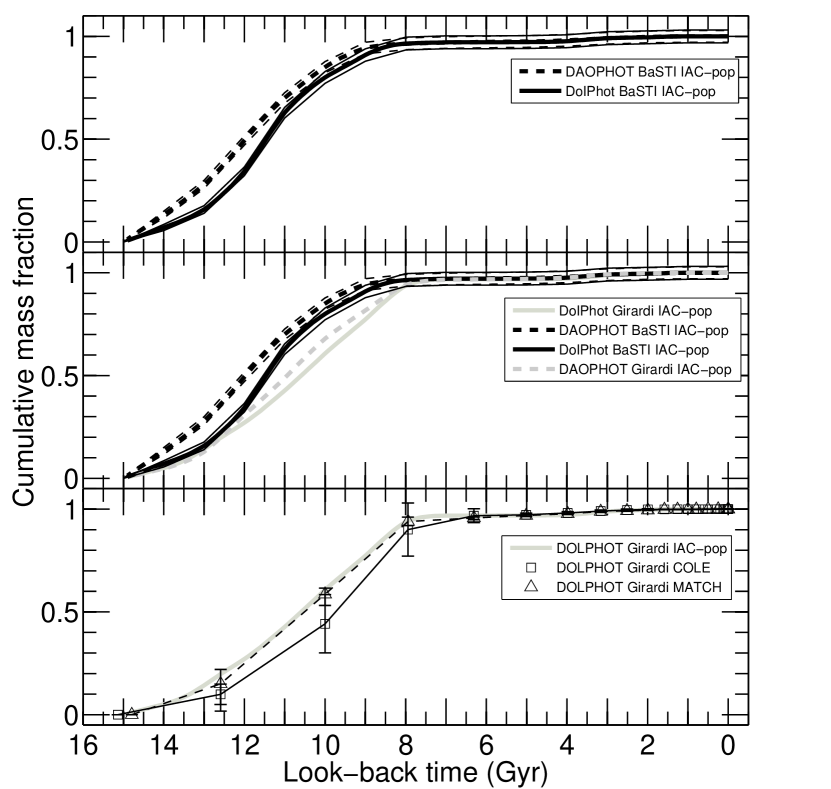
Figure 11.— Summary of the different results applying different techniques to derive the SFH. The cumulative mass fraction as a function of time is shown. Top: Comparison of the SFH derived with the MinnIAC/IAC-pop method, using the BaSTI library and the DAOPHOT and DOLPHOT photometry. The DAOPHOT SFH is overall less than 1 Gyr older then the DOLPHOT one. Middle: The same solutions are compared to analogous ones derived using the Padova/Girardi library. These solutions are systematically younger than the BaSTI solutions, particularly at old epochs for the DAOPHOT photometry. Bottom: Comparison of two different SFH codes, applied to the DOLPHOT photometry in combination with the Padova/Girardi library.

4.3. The COLE method

The third method we applied to measure the SFH of Cetus is a simulated annealing algorithm applied to our DOLPHOT photometry and the Padova/Girardi library. The code is the same as that applied to the galaxies Leo A (Cole et al., 2007) and IC 1613 (Skillman et al., 2003), and details of the method can be found in those references. The technique treats the task as a classic inverse problem by finding the SFH that maximizes the likelihood, based on Poisson statistics, that the observed distribution of stars in the binned CMD (Hess diagram) could have been drawn from the model.

The code uses computed stellar evolution and atmosphere models that give the stellar colors and magnitudes as a function of time for stars of a wide range of initial masses and metallicities. The isochrone tables (Marigo et al., 2008) for each (age, metallicity) pair are shifted by the appropriate distance and reddening values, and transformed into a discrete color-magnitude-density distribution $\varrho$ by convolution with an initial mass function (see Chabrier, 2003, , their Tab. 1). and the results of the artificial star tests simulating observational uncertainties and incompleteness. The effects of binary stars on the observations are simulated by adopting the binary star frequency and mass ratio distribution from the solar neighborhood, namely 35% of stars are single, 46% are parameterized as “wide” binaries, i.e., the secondary mass is uncorrelated with the primary mass, and is drawn from the same IMF as the primary, and finally 19% of stars are parameterized as “close” binaries, i.e., the probability distribution function of the mass ratio is flat.The progeny of dynamical interactions between binaries (e.g., blue stragglers) are not modelled. The history of the galaxy is then divided into discrete age bins with approximately constant logarithmic spacing in order to take advantage of the increasing time resolution allowed by the data at the bright (young) end. The star formation history is then modelled as the linear combination of $\psi$(t,Z) that best matches the data by summing the values of $\varrho$ at each point in the Hess diagram. The best fit is found via a simulated annealing technique that converges slowly on the maximum-likelihood solution without becoming trapped in local minima (such as those produced by age-metallicity degeneracy).

In our solution we considered only the DOLPHOT photometry. The critical distance and reddening parameters were held fixed at (m$-$M)₀ = 24.49 and and E(B$-$V) = 0.03. We used 10 time bins ranging from 6.60 $\leq$ log(age/Gyr) $\leq$ 10.18. Isochrones evenly spaced by 0.2 dex from $-2.3\leq[M/H]\leq-0.9$ were used, considering only scaled-solar abundances but with no further constraints on the age-metallicity relation. The CMD was discretized into bins of dimension 0.10$\times$0.20 mag, and it is the density distribution in this Hess diagram that was fit to the models. The error bars are determined by perturbing each component of the best-fit SFH in turn and re-solving for a new best fit with the perturbed component held fixed. The size of the perturbation is increased until the new best fit is no longer within 1$\sigma$ of the global best fit.

4.4. Comparison of the different solutions

Fig. 11 summarizes the comparison of the solutions calculated using different sets of photometry, stellar evolution libraries, and SFH codes.

The upper panel shows the cumulative mass fraction, as a function of time, based on the BaSTI library + IAC method applied to the two sets of photometry. The solution based on the DOLPHOT photometry is marginally younger than the DAOPHOT one. It shows slightly lower star formation at older epochs, and a steeper increase around 12 Gyr ago. In either case Cetus completely stopped forming stars $\sim$ 8 Gyr ago.

The middle panel compares the same two curves with analogous ones obtained using the Girardi library. The effect of changing the library introduces a small systematic effect; both solutions with the Girardi library shift more star formation to slightly ($\leq$ 1 Gyr) younger ages compared to the solutions using the BaSTI library. This effect seems more evident at the oldest epochs in the case of the DAOPHOT solutions.

The bottom panel shows the results of the three different SFH reconstruction methods, applied to the same photometric catalog and with the same stellar evolution library. Since for the MATCH and COLE method we present the result of the best individual solution, and not the average of many as in the case of the IAC method, the large dots highlight the centers of the age bins adopted. Note the good agreement between the MATCH and COLE with the IAC solution, in spite of the higher time resolution of the latter.

For simplicity, we will now focus our analysis on the SFHs obtained with the IAC method and the BaSTI stellar evolution library. At this time, we favor using the BaSTI stellar evolution library because the input physics has been more recently updated, in comparison to the Girardi stellar evolution library (Pietrinferni et al., 2004). Similarly, the IAC method will be used preferentially because it was tailored to the needs of this project and affords a greater degree of flexibility for the analysis (Hidalgo et al., in prep.).

5. The SFH of Cetus

In this section we present the details of the Cetus SFH. First, in §5.1, we describe the analysis we did to explore the possible systematics affecting the solution. We then describe our final solution in §5.2.

5.1. Approaching the best solution

5.1.1 Exploring the zero points systematics

Fig. 12 shows the grid of color and magnitude shifts adopted to derive the IAC-pop solution. The plus signs mark the positions of the 25 initial points. In each of these 25 positions we calculated the mean $\chi^{2}_{\nu}$, averaging the $\chi^{2}_{\nu}$ of the 24 individual solutions. This allows us to study how the $\chi^{2}_{\nu}$ varies as a function of the magnitude and color shifts. In particular, the minimum averaged $\chi^{2}_{\nu,min}$ identifies the position corresponding to the best solution, which is calculated by MinnIAC averaging the corresponding 24 individual solutions.

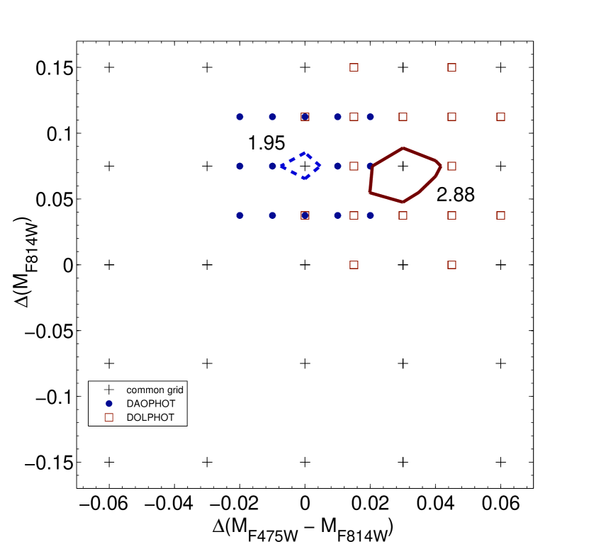
Figure 12.— Summary of the solutions derived as a function of the shifts in color and magnitude, $\delta_{col}$ and $\delta_{mag}$, applied to the observed CMD. In each position of the grid we calculated 24 solutions. Crosses mark the initial grid, common to both photometry sets. Filled circles and open squares show the sub-grid around the initial minimum, for the DAOPHOT and DOLPHOT photometry set, respectively. The two curves show the 1-$\sigma$ confidence area, defined using the dispersion of the 24 individual solution around the mean $\chi^{2}_{\nu}$.

Because the initial color and magnitude shifts are relatively large, we calculated more solutions on a finer grid with 14 positions around the identified minimum $\chi^{2}_{\nu}$ (Fig. 12, full circles and open squares for the DAOPHOT and DOLPHOT solution, respectively). Therefore, we obtained a total of (25+14)*24=936 solutions. This computationally expensive task was made possible by the Condor workload management system (Thain et al., 2005) available at the Instituto de Astrofísica de Canarias. In the case of the DAOPHOT photometry, the minimum was confirmed at the position ($\delta_{col}$ ; $\delta_{mag}$) = (0.0 ; 0.075), $\chi^{2}_{\nu,min}$ = 1.95, while in the case of the DOLPHOT photometry the minimum is located at ($\delta_{col}$ ; $\delta_{mag}$) = (+0.03, 0.075), $\chi^{2}_{\nu,min}$ = 2.88. The two curves around the minimum position of Fig. 12 represent the 1-$\sigma$ confidence area around the minimum, calculated as the dispersion around the mean of the 24 $\chi^{2}$ of the individual solutions (Aparicio & Hidalgo, 2009). Note that the color difference between the $\chi^{2}_{\nu,min}$ of the two photometry sets is fully consistent with, and apparently compensates for, the color shift between the two photometry sets ($\sim 0.04$ mag). This indicates that the flexibility of our method is able to deal with subtle photometric calibration systematics, and possible stellar evolution model, distance, and reddening uncertainties.

Fig. 13 shows a direct comparison between the 24 individual DAOPHOT and DOLPHOT solutions at the $\chi^{2}_{\nu,min}$ position. The horizontal lines show the size of the age bins, and do not represent error bars. It is noteworthy that the spread of the 24 solutions, derived using different input samplings, is quite small, suggesting the robustness of the mean SFH. Note also the good agreement between the solutions from the two photometry sets. The general trend is the same, with the main peak of star formation occurring within $\sim$ 0.5 Gyr and, most importantly, characterized by the same duration.

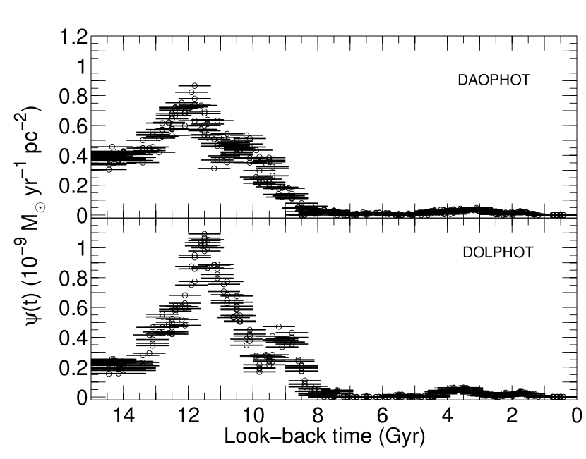
Figure 13.— Comparison of the 24 individual DAOPHOT and DOLPHOT solutions at the best $\chi^{2}_{\nu}$ position, from both sets of photometry. Note the stability of the solution against small changes of the input bins adopted. Moreover, the plot puts into evidence the similarity of the solutions obtained from the DAOPHOT and DOLPHOT photometry. Note that the horizontal lines are not the error bars, but represent the size of the age bin.

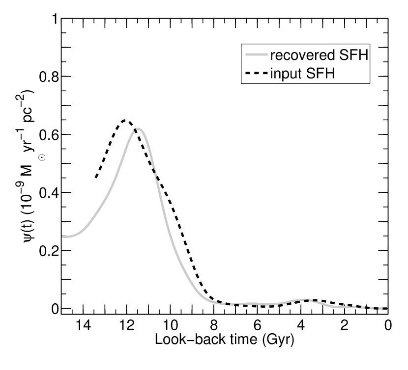
Figure 14.— Results of a test designed to investigate the significance of the oldest $\psi(t)$ in our solutions. Dashed line: input SFH, adopted as our Cetus solution, but removing all stars older than 13.5 Gyr. Solid line: recovered SFH when using a model CMD that contains stars as old as 15 Gyr. A low level of star formation is recovered for ages older than 13.5 Gyr, when there should be none.

5.1.2 The age of the oldest stars

Another important aspect to be addressed is the occurrence of star formation at epochs older than 14 Gyr. As discussed in §4.1, we did not impose any strong constraints on the ages of the oldest stars in the model used to derive the SFH of Cetus. That is, we let the code search for the best solution using model stars as old as 15 Gyr, significantly older than the age of the Universe commonly accepted after the WMAP experiment (Bennett et al., 2003). Interestingly enough, our solution shows very low star formation rate for epochs older than 14 Gyr, with a steady increase toward a peak at $\sim$ 12 Gyr.

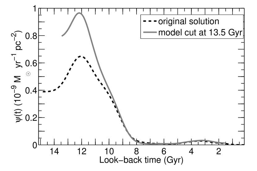
Figure 15.— Comparison between the Cetus $\psi(t)$ obtained using a model CMD with constant SFR up to 15 (dashed black line) and and up 13.5 Gyr (solid grey line).

To further investigate the significance of deriving ages of stars older than 14 Gyr, we performed the following test. Using the derived SFH, we calculated a synthetic CMD, from which we removed all the stars older than 13.5 Gyr. We simulated the observational errors and then derived the SFH of this new CMD identically as for Cetus. Fig. 14 presents the input and recovered $\psi(t)$. The latter shows some level of star formation at epochs older than 13.5 Gyr, when there should be none. This means that the combination of observational errors and the uncertainties associated with the SFH algorithms is responsible for the smearing of the main peak of star formation at the oldest epochs.

Therefore, we decided to adopt the external constraint on the age of the Universe coming from the cosmic microwave background experiments, and we set the upper limit to the model stars’ age to 13.5 Gyr. This choice is also supported by the fact that current stellar evolution models give Milky Way globular cluster ages in very good agreement with this estimated age of the Universe (Marín-Franch et al., 2009). The effect of this constraint is shown in Fig. 15. The main effect of limiting the age of the oldest stars in the synthetic reference CMD is that the peak of star formation is higher (since total star formation must be conserved). However, there is no effect on the age or the end of the main episode of star formation, nor on the star formation at epochs younger than 10 Gyr. With both models, we calculate that Cetus completely stopped forming stars $\sim$ 8 Gyr ago. This test was repeated with both the DAOPHOT and DOLPHOT solutions, leading to the same conclusion. Thus, we adopt this constraint on the SFH for the rest of our analysis.

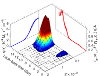
Figure 16.— 3-D representation of the Cetus SFH, derived with the DAOPHOT (top) and the DOLPHOT (bottom) photometry. Both show the average of 24 solutions calculated at the minimum $\chi^{2}_{\nu}$ in the $\delta mag$-$\delta col$ grid. The $\chi^{2}_{\nu,min}$ is 2.18 and 2.92 for the DAOPHOT and DOLPHOT solutions, respectively.

Figure 17.— Summary of the Cetus SFH results. The three panels represent, from top to bottom, the $\psi(t)$, the age-metallicity relation and the cumulative mass fraction. We show the results with the BaSTI library for both the DAOPHOT (dashed line) and the DOLPHOT (continuous) photometry, and the average of the two (thick cyan line). The dashed part of the cyan line representing the average of the two sets of photometry in the middle panel indicates the presence of BSs rather than a low level of intermediate-age and young SF. The thin lines represent the error bars, while the vertical lines in the upper panel mark redshift z $=$ 15 and 6, that is the epochs corresponding to the reionization. (Bouwens et al., 2007). The dotted-dashed lines in the central panel mark the epochs when 10%, 50% and 90% of the mass was formed.

5.2. The final SFH of Cetus

The solutions for each set of photometry, calculated as the average of the 24 solutions at the $\chi^{2}_{\nu,min}$, are represented in Fig. 16 where a 3-D smoothed histogram summarizes the main features. This is a useful representation giving an overall view of the SFH of a system (Hodge, 1989), including the star formation rate as a function of time, the metallicity distribution function and the age-metallicity relation. It shows graphically how the oldest stars are more metal-poor, and how chemical enrichment proceeds toward younger ages. The two projections $\psi(z)$ and $\psi(t)$ are the metallicity distribution integrated over time (blue line) and the age distribution integrated over metallicity (red line). Errors have been calculated for $\psi(t)$ and $\psi(z)$ as the dispersion of the 24 individual solutions used in the average (see Aparicio & Hidalgo, 2009). In particular, the $\psi(z)$, shows a peak at the most metal poor regime, and a sharp decrease toward the more metal-rich tail. Only a negligible fraction of stars ever formed have metallicities higher than Z=10^-3.

The overall agreement between the DAOPHOT and the DOLPHOT solutions, illustrated in Fig. 13 and in Fig. 16 suggests that we can safely adopt the average of the two solutions for the SFH of the Cetus dSph galaxy, and the difference of the two as an indication of external errors .

Fig. 17 summarizes the main results by comparing the star formation rate as a function of time (top), the age-metallicity relation (middle), and the cumulative mass function (bottom), for both sets of photometry with the adopted average calculated as explained in Hidalgo et al., in prep. The thick dashed and continuous lines represent the DAOPHOT and DOLPHOT solutions, while the thin lines are the corresponding error bars, calculated as the 1-$\sigma$ dispersion of the 24 solutions at $\chi^{2}_{\nu,min}$. This is a statistically meaningful way of defining the uncertainities introduced by the SFH recovery method, as extensively discussed in Aparicio & Hidalgo (2009). The thick cyan line is the average of the solutions obtained for the two photometries. Fig. 16 and Fig. 17 provide two complementary ways of presenting the derived SFH of Cetus. From these figures we see that Cetus is mostly an old, metal-poor stellar system, with the vast majority of stars older than 8 Gyr and more metal-poor than Z = 0.001. Tab. 1 summarizes the main integrated quantities derived for both photometry sets.

Table 1Integrated quantities derived for the Cetus dSph.

	DAOPHOT	DOLPHOT
$\int\psi(t)dt$ $[10^{6}M_{\odot}]$	(1.81$\pm$0.05)	(1.91$\pm$0.07)
$<\psi(t)>[10^{-7}M_{\odot}yr^{-1}pc^{-2}$]	(1.17$\pm$0.02)	(1.23$\pm$0.03)
$<age>[10^{10}yr]$	(1.14$\pm$0.02)	(1.12$\pm$0.02)
$<[Fe/H]>[10^{-4}dex]$	(4.23$\pm$0.54)	(3.64$\pm$0.53)

The vertical lines in the top panel indicate the redshift $z$ = 15 and $z$ = 6, which mark the epoch when reionization was under way, the latter considered to be the epoch when the Universe was fully reionized (Bouwens et al., 2007, and references therein). The vertical lines in the middle panel of Fig. 17 mark the epoch when 10, 50 and 90% of the stellar mass was formed. They indicate that Cetus experienced the bulk of its star formation before redshift $\approx 2$, with a peak at $z\sim 4$.

In the following, we focus on two important aspects of the Cetus SFH: the sequence of candidate BSs and the actual duration of the main episode of star formation.

5.2.1 Recent star formation or blue stragglers

In §3 we gave circumstantial evidence, based on the comparison with isochrones, that the objects bluer and brighter than the old MSTO are BSs, rather than truly young stars. More evidence of this comes from the analysis of the SFH presented in 16. The plot shows an event of very low SFR that produced a small percentage of metal-poor but relatively young ($\sim$ 2-4 Gyr old) stars. This population clearly does not follow the general age-metallicity relation. Fig. 18 shows that the position of these stars in the solution CMD is fully consistent with the position of the blue plume on the CMD. This feature is systematically present in all our solutions, and does not depend on the sampling, library, or photometry adopted. Given the age-metallicity relation derived for Cetus, there is no reason to expect a relatively young but very metal-poor population - this would require something like an episode of late infall of very metal poor gas. This interpretation is nicely supported by the age-metallicity relation presented in Fig. 17 (middle panel), which shows a continuous increase of metallicity with time, until a peak occurs 8 Gyr ago. After that, we observe a sharp decline followed by a renewed increase. If we accept that blue stragglers are found in all or nearly all sufficiently populous open and globular star clusters as well as in the Milky Way field halo population, then there is no conflict between our data and the assertion that no star formation occurred in Cetus in the last 8 Gyr; the most natural explanation for these stars is that they are blue stragglers belonging to the old, metal-poor population. Note that the contribution of BS to the total estimated mass of Cetus is $\leq 3\%$. Therefore, the presence of fainter BSs contaminating the TO and MS regions is expected to have negligble impact on the derived SFH. An in-depth discussion of the candidate BSs in both dSph galaxies of the LCID sample will be presented in a forthcoming paper (Monelli et al., in prep.)

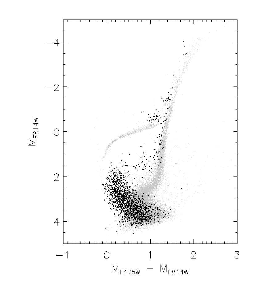
Figure 18.— Syntetic CMD corresponding to the SFH of Cetus. The young metal-poor stars are highlighted with bigger points. Their position on the CMD is fully consistent with the candidate BSs sequence.

5.2.2 The short first episode of SFH in Cetus

The description presented in §5 corresponds to the SFH of Cetus as derived using the discussed algorithms. It is clear that this solution is the result of the convolution of the actual Cetus SFH with some smearing produced by the observational errors, and the limitations of the SFH recovery method (Aparicio & Hidalgo, 2009). In the following, we will try to further constrain the features of the actual Cetus SFH through some tests with mock stellar populations.

To investigate the actual duration of the dominant episode of star formation, and to assess the age resolution at the oldest ages, we performed the following test. We created mock galaxies characterized by fixed metallicity and short episodes of star formation around the mean value of 12.0 Gyr (see Fig. 19). Since a Gaussian profile fit to the Cetus $\psi(t)$ yields an estimate of $\sigma=1.53$ Gyr, we used three $\psi(t)$ modeled by a Gaussian profile with $\sigma=0.5$, $1.0$, and 1.5 Gyr. We simulated the observational errors in the mock stellar populations, and recovered their SFH using the same prescriptions as for the real data. For simplicity, only the completeness tests of the DAOPHOT photometry were adopted to simulate the observational errors in the mock CMD. The number of stars in the mock populations was such that the total number of stars in the bundles was comparable to the case of the real galaxy.

The first important result of this test is that the age of the peak of the recovered mock population is systematically well recovered, within 0.2 Gyr. Thus, if the initial episode of star formation in Cetus is well represented by a Gaussian profile, then we are confident in our ability to determine the time of the peak star formation rate. Similar tests have been also discussed in Aparicio & Hidalgo (2009) and Hidalgo et al., in prep. The second finding is that the duration of the recovered $\psi(t)$ is wider than the input one. In particular, we measured the HWHM and calculated the corresponding $\sigma$, which are equal to 1.44, 1.61, and 1.95 Gyr for the three episodes of increasing duration. The increase from the input $\sigma$ is a consequence of the blurring effect of the observational errors and the limited age resolution at old ages.

The comparison of the duration of the main peak in the Cetus and in the mock stellar populations suggests that the estimated duration for Cetus is an upper limit. Moreover, we note that this value can be further constrained by the $\sigma=0.5$ and the $\sigma=1.0$ Gyr Gaussian profile tests, with a result close to $\sigma=0.8$ Gyr (interpolated value). Moreover, we can expect that the limited age resolution broadens both the older and the younger sides of the $\psi(t)$, around its maximum. This is supported by Fig. 19, where we can compare the youngest epoch of star formation in the three models and in their recovered profiles. The comparison reveals that the output $\psi(t)$ is more extended to younger ages than the input ones, and that this effect is less important for increasing $\sigma_{in}$. This suggests that at least part of the star formation between 10 and 8 Gyr ago derived in Cetus is not real. However, we stress that the differences between the actual SFH and the recovered one affect only the duration of the star formation solution and the height of the main peak, but they do not alter significantly the age of the peak itself.

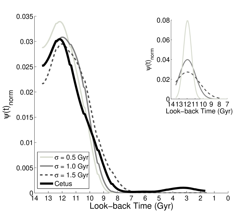
Figure 19.— Comparison of the $\psi(t)$ derived for Cetus with that retrieved from three mock stellar populations. These were computed with a Gaussian profile $\psi(t)$ with $\sigma=$0.5, 1.0, and 1.5 Gyr peaked at 12 Gyr, as shown in the small top-right panel. The recovered $\psi(t)$ is wider than the input one. This test indicates that the intrinsic duration of the main star formation episode in Cetus can be confined between the $\sigma=$0.5 and $\sigma=$1 Gyr. All the curves presented are normalized to their total area.

Finally, Fig. 20 presents a comparison between the observed DAOPHOT CMD and a synthetic CMD corresponding to the best solution (left and cetral panels). We find a satisfactory agreement in all the main evolutionary phases, including the RGB phase which has not been used to derive the solution. As far as it concerns the differences in the HB morphology, it is worth noting that we have not tried to properly reproduce this observational feature. Due to the strong dependence of the HB morphology on the mass loss efficiency along the RGB, it is clear that a better agreement between the observational data and the synthetic CMD could be obtained with a better knowledge of mass loss efficiency and its spread. The right panel shows the residual Hess diagram, which supports the good agreement between the observed and the solution CMD.

Figure 20.— Comparison of the observed (left) and solution (centre) CMDs. The latter was derived extracting random stars from the model CMD used to derive the solution, in such a way that each simple population contributes proportionally to the calculated SFR. The rigth panels shows the residual Hess diagram, shown in unit of Poisson errors. The Figure disclose an overall general agreement between the observed and the solution CMDs, particularly in the whole TO region used to calculate the SFH. The discrepancy at the faintest magnitude is due to the limit magnitude of the model CMD. Note that such discrepancy does not affect the portion of the CMD included in the bundles, which are repeated in the left panel. The differences in the HB morphology are expected, since small differences in the adopted mass-loss along the RGB have a big impact on the HB morphology.

5.3. Are we seeing the effects of reionization in the Cetus SFH?

One of the main drivers of the LCID project is to find out whether cosmic reionization left a measurable imprint on the SFHs of nearby, isolated dwarf galaxies. The Universe is thought to have been completely reionized before z $\geq$ 6 (Bouwens et al., 2007), corresponding to T $\simeq$ 12.8 Gyr ago. The comparison of these values with the Cetus $\psi(t)$ in Fig. 17 (see upper panel), shows that the vast majority of the measured star formation in Cetus occurred at epochs more recent than 12.8 Gyr ago (see also Tab. 2). This is also true when the actual Cetus SFH is considered, as discussed in section 5.2.2. Therefore, we conclude that there is no evident coincidence between the epoch when reionization was complete and the time in which the star formation in Cetus ended.

However, one might ask the question of whether acceptable solutions could be found that don’t show star formation more recent than 12.8 Gyr ago, i.e., that are compatible with the hypothesis that reionization contributed to the supression of star formation in Cetus. With this question in mind, we performed two additional tests, summarized in Fig. 21.

$\bullet$ First, we calculated a solution SFH of Cetus costraining the model CMD to stars of ages older than 12.8 Gyr. This is not the typical approach for the IAC method, but nontheless the code looks for the absolute minimum in the allowed parameter space, and provides the best possible solution (grey dashed line). However, we found that this solution is clearly at odds with the derived best SFH of Cetus, and not compatible with it. Also, note the significantly higher $\chi^{2}_{\nu}$, which increases to 7.80, and the large residuals (Fig. 21, central panel). The latter, calculated with respect to the observed CMD identically as in Fig. 20, indicate important systematics in the solution. The excess of stars in the solution CMD in the red part of the TO (lightest bins), indicates the presence of too many stars in this region. This is in agreement with the overall older population, with the main peak at $\sim$ 13 Gyr ago.

$\bullet$ We recovered the SFH of a mock population, similarly to the tests shown in Fig. 19, created with constant SFR in the age range between 13 and 13.5 Gyr, and zero elsewhere. The solution shown in Fig. 21, discloses that the peak is recovered at the correct age, in the oldest possible age bin (grey solid line). This suggests that an actual SFH where most of stars were born before the end of the reionization epoch is not compatible with the solution we derived for Cetus. Moreover, the general trend in the residual plot (Fig. 21, right panel), is similar to the previous case, with an excess of red TO stars.

These two tests, together with the ones shown in Fig. 19, suggest that, on the basis of the available data coupled with the SFH recovery code, we can reject the hypothesis that the majority of the star formation occurred in Cetus in epochs older than z $\simeq 6$.

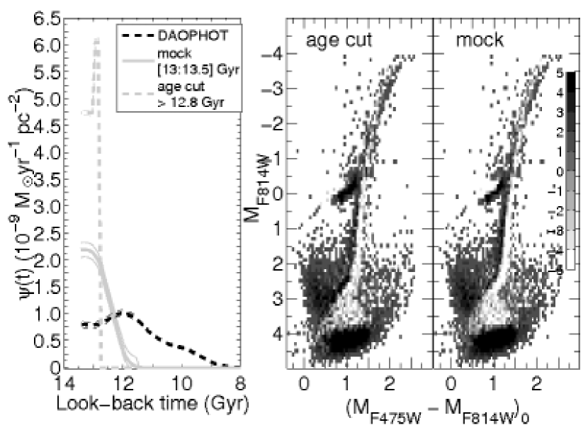
Figure 21.— The left panel compares the $\psi(t)$ of Cetus (black dasked line) to (i) the one of a mock population, created with stars in the range between 13 and 13.5 Gyr (solid grey line), and (ii) a solution derived for Cetus, but imposing the constraint to use only stars older the 12.8 Gyr (dashed grey line). The central and right panels show the residual Hess diagram of these two solutions, calculated identically as in Fig. 20. The residual CMDs show important systematics suggesting that these solutions are not compatible with the derived best solution of Cetus, thus supporting that no strong correlation exists between the epoch of the reionization and the epoch of the star formation in this galaxy.

5.4. Summary

The various pieces of information analysed in the §5 can be sumarized as follows. The star formation of the observed area of Cetus shows a well-defined peak that occurred $\approx$ 12 Gyr ago. By resolving the star formation of mock stellar populations, we showed that the actual duration of the main event is probably overestimated, due to the smearing effect of the observational errors. This does not affect the age of the main peak, but only its duration, at both older and younger epochs. Therefore, the last epoch of star formation, estimated at 8 Gyr ago, is probably actually somewhat older. The various evidence indicating that the blue plume of objects identified in the CMD consists of a population of BS, supports the idea that no star formation occurred in Cetus in the last 8-9 Gyr. In Tab. 2 we present the epoch when various fractions of the total mass were formed, once we excluded the contribution of the BS population. However, the actual values of the percentiles reported could be slighlty different due to the smearing of the solution with respect of the actual, underlying SFH (see §5.2.2).

The derived SFH is at odds with the conclusion by Sarajedini et al. (2002), who suggested that Cetus might be 2-3 Gyr younger that the old Galactic globular clusters. The stability of the main peak around the age of 12 Gyr, together with up-to-date estimates of the globular cluster ages (Marín-Franch et al., 2009), suggest that such a difference can be ruled out.

Table 2Mass percentiles formed in Cetus as a function of redshift and look-back time.

Mass %	redshift	Look-Back Time (Gyr)
10	8.8	13.1
20	5.7	12.7
30	4.5	12.3
40	3.7	12.0
50	3.2	11.6
60	2.8	11.3
70	2.4	10.9
80	2.0	10.4
90	1.7	9.7

6. Discussion

The SFH of Cetus derived in this paper shows that this dSph was able to form the vast majority of its stars coincident with and after the epoch of reionization. Furthermore, there are no signs in the SFH suggestive of a link between a characteristic time in the SFH and the time of reionization. This may be due to the fact that Cetus, with a velocity dispersion of $\sigma=$ 17 $\pm$ 2 km/s (Lewis et al., 2007), is one of the brightest ($M_{V}\sim-10.1$, Whiting et al. 1999), and presumably one of the most massive dSphs in the Local Group. Its large mass might therefore have shielded its baryonic content from the effects of reionization (Barkana & Loeb, 1999; Carraro et al., 2001; Tassis et al., 2003; Ricotti & Gnedin, 2005; Gnedin & Kravtsov, 2006; Okamoto & Frenk, 2009). The latter reference, in particular, argues that all classical LG dwarfs originate in the few surviving satellites which, at the time of reionization, had potential wells deeper than the threshold value of $\sim 12$ km/s. If reionization by the UV background cannot be related to the early truncation of star formation in Cetus, then other circumstances must be at play. According to the model by Okamoto & Frenk (2009), the sudden truncation in the SFH of dwarfs like Cetus arises from having their gas reservoirs stripped during first infall into the potential wells of one of the massive LG spirals (M31 or MW). Another possibility frequently raised in the literature is that the end of star formation reflects the blow-out of gas driven by supernova explosions. We examine each of these two possibilities below.

The radial velocity of Cetus measured by Lewis et al. (2007) implies that this galaxy is receding with respect to the Local Group barycenter and, under reasonable assumptions about its proper motion and the mass distribution in the Local Group, that it is close to the apocenter of its orbit. Therefore, it is possible that Cetus is in a highly radial orbit and that it has gone through pericenter at least once. If this was the case, then it is possible that the truncation of the star formation occurred due to the effect of tides and ram-pressure (Mayer et al., 2001; Okamoto & Frenk, 2009) during pericentric passage. The mild evidence of rotation found by Lewis et al. (2007) may be interpreted to imply that the progenitor of Cetus was a disk-like dwarf that underwent an incomplete transformation into a spheroidal system as a result of the strong tides operating at pericenter (Mayer et al., 2001; Lokas et al., 2009). The models by Lokas et al. (2009) predict different final configurations after one passage for a disky dwarf. Depending on the geometry of the encounter, either a triaxial, rotating system or a prolate object with little rotation may result. Alternatively, it has been proposed by D’Onghia et al. (2009) that a gravitational resonance mechanism, coupling the rotation of the accreting disky dwarf with its orbital motion, is able to turn it into a dSph in a single encounter. However, this requires a nearly prograde encounter. The latter condition may not be common during the hierarchical assembly of the galaxy, but may still have occurred in just a few cases (prograde accretions are seen in cosmological hydrodynamical simulations) which would be enough to explain the small subset of distant dSphs. A firm measure of the shape of Cetus might thus be an important step in the context of constraining its formation models. Independently of the mechanism driving the encounter, if Cetus has indeed been through the pericenter of its orbit, it is possible that it owes its present-day isolation in the LG to the fact that it gained orbital energy in the process and is now on a weakly bound orbit that takes it well beyond the normal confines of the LG. This possibility has been highlighted by Sales et al. (2007) and Ludlow et al. (2009), who discuss the possibility that the odd orbital motion of Cetus might have originated in a multiple-body interaction during pericenter.

On the other hand, models of the SFH in dwarfs driven by feedback are also able to reproduce the main properties of dSph galaxies without invoking galaxy interactions. In particular, Carraro et al. (2001) find that the key parameter is the dwarf’s central density, while Sawala et al. (2009) argue that, as in previous models such as Mac Low & Ferrara (1999), low-mass systems are those most likely to end up as dSph galaxies. However, despite some differences all models of gas blow-out by supernova explosions find the mechanism to be inefficient above $10^{7}M_{\odot}$. While ultra-faint dwarfs may well be in the right mass regime, this is a problem for all classic dSphs since their initial masses were likely at least two orders of magnitude above this threshold (Mayer, 2009). Note also, that models of dSph formation that are based only on galaxy mass and feedback are unable to reproduce the morphology-density relationship.

When compared to the dSph satellites of the Milky Way, the stellar content of Cetus shows striking similarities with the Draco dSph. Aparicio et al. (2001), on the basis of a ground-based CMD of depth similar to those obtained by LCID for more distant dwarfs, concluded that most of its star formation occurred more than 10 Gyr ago, and that Draco stopped forming stars $\sim$ 8 Gyr ago. They also infer a less intense episode $\sim$3-2 Gyr ago, which is reminiscent of the population in Cetus that we associate with blue stragglers. Therefore, Cetus’s SFH looks more similar to that of other nearby dSphs with mostly old stellar populations, such as Draco, Ursa Minor, Leo I, Sculptor or Sextans. Their SFHs differ from those of other dSphs like Carina, Fornax or Leo II, where there is clear evidence for a substantial intermediate-age population. The striking observation that Cetus and Tucana (the other isolated LG dSph) do not follow the morphology-density relation of Milky Way dSph galaxies observed in the LG today appears to be simply an observational coincidence. Their radial velocities indicate that it is possible that they were much closer to the dominant LG spirals when their SF ceased, indicating that their star formation might have been truncated by the same mechanism responsible for the formation of the other LG dSphs.

7. Summary and conclusions

We used HST/ACS observations to derive the SFH of the isolated Cetus dSph. This effort is part of the LCID project, whose main goal is to investigate the SFH of isolated dwarf galaxies in the LG. To asses the robustness of our conclusions, the LCID methodology uses and compares the results of two photometric codes, two stellar evolution libraries, and three SFH-estimation algorithms. This allowed us to check the stability of our solution, and to give a robust estimate of the external errors affecting it (see also Hidalgo et al., in prep.). The use of different stellar evolution libraries and/or SFH codes does not change the global picture we derived. We found that the BaSTI library gives solutions systematically older (less than 1 Gyr) than the Padova/Girardi one. The cumulative mass fraction showed in Fig. 11, comparing the different solutions shows a good general agreement within the error bars. Finally, the good consistency of the SFH solutions derived with the DAOPHOT and DOLPHOT photometry sets warranted to adopt the average of the two solutions as the final Cetus SFH.

Our main result is that Cetus is an old and metal-poor system. We find evidence for Cetus stars as old as those in the oldest populations in the Milky Way, and comparable in age to the age of the Universe inferred from WMAP (Bennett et al., 2003). Star formation decreased after the earliest episode which likely peaked about $\sim$ 12 Gyr ago. We find no convincing evidence for a population of stars younger than $\sim 8$ Gyr old.

A number of tests aimed at recovering the SFH of mock stellar populations yield a estimate of our precision for determining the peak of star formation of the order of $\leqslant$ 0.5 Gyr for a given stellar evolution library. Therefore, our estimate that the Cetus peak $\psi(t)$ occurred $\sim$ 12 Gyr ago, is a robust result. Our tests also disclosed that the measured duration of the star formation is artificially increased by the observational errors. We could estimate that the intrinsic extent is compatible with an episode approximated by a Gaussian profile with $\sigma=$ 0.8 Gyr (or 1.9 Gyr FWHM), as opposed to the measured $\sigma=1.53$ Gyr. This likely moves the end of the star formation at older epochs.

The age-metallicity relation shows a mild but steady increase in metallicity with time, up to $Z=0.001$. The presence of bright, blue stars in the upper main sequence formally implies a sprinkling of stars younger than $\sim 8$ Gyr old. These stars, however, are inferred to have metallicities below $Z=0.001$, and thus would be clear outliers in the monotonic age-metallicity relation. An alternative interpretation, which we favor, is that these are not younger main-sequence stars but rather a population of blue stragglers with the same typical metallicity as the bulk of the population in Cetus.

In conclusion, we do not find any direct correlation between the epoch of the reionization and the epoch of the star formation in Cetus. In particular, the reionization does not seem to have been an efficient mechanism to stop the star formation in this galaxy. Alternative mechanisms, such as gas stripping and tidal interactions due to a close encounter in the innermost regions of the LG, seem favored with respect of internal processes like supernovae feedback.

.1. The effect of binary stars

To study the impact of different assumptions on the binary content of the model CMD, we used the IAC method to the identically derive the SFH with six different synthetic CMDs, varying the amount of binary stars from 0% to 100%, in steps of 20%. In all cases, we adopted a mass ratio between the two components $q>0.5$, and a flat mass distribution for the secondary. Fig. 22 summarizes the $\chi^{2}_{\nu,min}$ as a function of the binary fraction for five out of the six galaxies of the LCID sample, based on the DAOPHOT photometry: Cetus, Tucana, LGS 3, IC 1613, and Leo A. The five galaxies show a common general trend: the $\chi^{2}_{\nu}$ decreases for increasing number of binaries, and reaches a plateau and possibly a minimum around 40% – 60%. We conclude that we cannot put strong constraints on the binary content of these galaxies on the basis of these data, although a very low binary content seems to be disfavored.

The impact of different amount of binaries on $\psi(t)$ is shown in Fig. 23, where we plot the cumulative mass fraction and the $\psi(t)$ for the six different assumptions of the binary stars applied to the DAOPHOT photometry of Cetus. We detect a mild trend, the solution getting slightly younger for increasing amount of binaries. This is shown also in the bottom panel of the same figure, where the $\psi(t)$ tends to be more extended to younger ages for increasing binary fraction. However, the main features are not strongly affected by the assumptions made on the characteristics of the binary star population. In particular, the age of the main peak of star formation is stable within $\sim$ 0.6 Gyr.

Moreover, we show that the position of the minimum in the $\chi^{2}_{\nu}$ plot as a function of $\delta_{col}-\delta_{mag}$, changes as a function of the assumed binary content. As a general trend, we found that for increasing binary content, the minimum $\chi^{2}_{\nu}$ tends to migrate toward redder color and shorter distance, as summarized in Tab. 3 in the case of Cetus. This can be easily understood in terms of how the increasing number of binaries changes the distribution of stars in the model CMD. The higher the binaries content, the redder and more luminous the MS and MSTO.

Table 3Integrated quantities derived for the Cetus dSph.

Bin. %	Best $\chi^{2}_{\nu}$	$\Delta col-\Delta mag$	$\chi^{2}_{\nu}$at (0;0)
0	2.60$\pm$0.03	(-0.020 ; +0.1125)	4.53
20	2.18$\pm$0.04	(-0.010 ; +0.075)	3.04
40	1.95$\pm$0.02	( 0.0 ; +0.075)	2.54
60	1.86$\pm$0.05	(+0.020 ; +0.075)	2.10
80	1.80$\pm$0.06	(+0.010 ; +0.0375)	1.88
100	1.75$\pm$0.05	(+0.020 ; +0.0375)	1.84

Figure 22.— Summary of the $\chi^{2}_{\nu}$ trend as a function of the binary fraction for 5 galaxies analyzed in the LCID project.

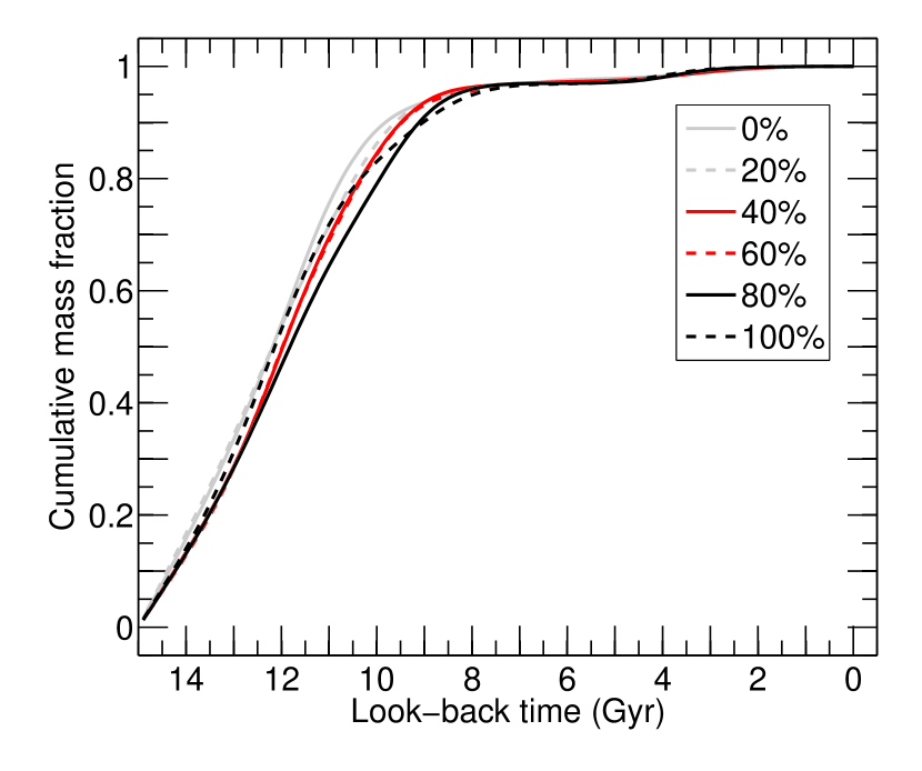
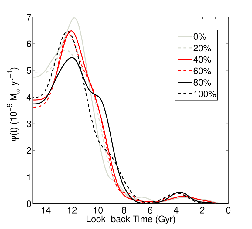
Figure 23.— Top: Cumulative mass fraction derived using model CMDs with six different percentages of binary stars. The amount of binaries slightly affects the solution, and we detect a mild tendency to recover slightly younger solutions for increasing amount of binaries. Bottom: The six corresponding $\psi(t)$ show that all the main features do not vary for different assumptions of binaries. Note that the main peak of star formation occur at the same age within $\sim$ 0.6 Gyr.

References

- Aparicio et al. (1997) Aparicio A., Gallart, C., & Bertelli, G. 1997 AJ, 114, 680
- Aparicio et al. (2001) Aparicio, A., Carrera, R, Martínez-Delgado, D. 2001, AJ, 122, 2524
- Aparicio & Gallart (2004) Aparicio, A., & Gallart, C. 2004, AJ, 128, 1465
- Aparicio & Hidalgo (2009) Aparicio, A., & Hidalgo, S. 2009, AJ, in press, arXiv:0906.0712
- Babul & Rees (1992) Babul, A. & Rees, M. J. 1992, MNRAS, 255, 346
- Barkana & Loeb (1999) Barkana, R. & Loeb, A. 1999, ApJ, 523, 54
- Bedin et al. (2005) Bedin, L., Cassisi, S., Castelli, F., Piotto, G., Anderson, J., Salaris, M., Momany, Y., Pietrinferni, A., 2005, MNRAS, 357, 1038
- Bennett et al. (2003) Bennett, C. L. et al., 2003, ApJS, 148, 1
- Bernard et al. (2009) Bernard E., et al. 2009, ApJ, 699, 1742
- Bertelli et al. (1992) Bertelli, G., Mateo, M., Chiosi, C., Bressan, A. 1992 ApJ, 388, 400
- Bouchard et al. (2006) Bouchard, A., Carignan, C., & Staveley-Smith, L. 2006, AJ, 131, 2913
- Bouwens et al. (2007) Bouwens, R. J., Illingworth, G. D., Franx, M., & Ford, H. 2007, ApJ, 670, 928
- Bullock et al. (2000) Bullock, J.S., Kravtsov, A.V., & Weinberg, D.H. 2000, ApJ, 539, 517
- Carraro et al. (2001) Carraro, G., Chiosi, C., Girardi, L., & Lia, C. 2001, MNRAS, 327, 69
- Cassisi et al. (1999) Cassisi, S., Castellani, V., Degl’Innocenti, S., Salaris, M., & Weiss, A. 1999, A&ASS, 134, 103
- Castellani et al. (1997) Castellani, V., Ciacio, F., Degl’Innocenti, S., & Fiorentini, G. 1997, A&A, 322, 801
- Chabrier (2003) Chabrier, G. 2003, PASP, 115, 763
- Chiba & Nath (1994) Chiba, M. & Nath, B. B. 1994, ApJ, 436, 618
- Cole et al. (2007) Cole, A. et al. 2007, ApJ659, 17
- Dolphin (2000a) Dolphin, A. E. 2000, MNRAS, 313, 281
- Dolphin (2000b) Dolphin, A. E. 2000, PASP, 112, 1383
- Dolphin (2002) Dolphin, A. E. 2002, MNRAS, 332, 91
- D’Onghia et al. (2009) D’Onghia, E., Besla, G., Cox, T., J., Hernquist, L. 2009, Nature, 460, 605
- Efstathiou (1992) Efstathiou, G. 1992, MNRAS, 256, 43P
- Ford et al. (1998) Ford, H. C., et al. 1998, Proc. SPIE, 3356, 234
- Gallart et al. (1996) Gallart, C., Aparicio, A., & Vilchez, J. M. 1996, AJ, 112, 1928
- Gallart et al. (1999) Gallart, C., Freedman, W. L., Aparicio, A., Bertelli, G., & Chiosi, C. 1999, AJ, 118, 2245
- Gallart et al. (2005) Gallart, C., Zoccali, M., & Aparicio, A. 2005, ARA&A, 43, 387
- Girardi et al. (2000) Girardi, L., Bressan, A., Bertelli, G., Chiosi, C. 2000, A&AS, 141, 371
- Gnedin & Kravtsov (2006) Gnedin, N. Y., & Kravtsov, A. V. 2006, ApJ, 645, 1054
- Harris & Zaritsky (2001) Harris, J. & Zaritsky, D. 2001, ApJS, 136, 25
- Hill et al. (1998) Hill, J.R. et al. 1998, ApJ, 496, 648
- Hodge (1989) Hodge, P. 1989, ARA&A, 27, 139
- Holtzman et al. (2006) Holtzman, J. A., Afonso, C., Dolphin, A. 2006, ApJS, 166, 534
- Hurley & Tout (1998) Hurley, J., & Tout, C. A. 1998, MNRAS, 300, 977
- Iben (1968) Iben, I. Jr. 1968, ApJ154, 581
- Ikeuchi (1986) Ikeuchi, S. 1986, Ap&SS, 118, 509
- Kepner, Babul, & Spergel (1997) Kepner, J. V., Babul, A., & Spergel, D. N. 1997, ApJ, 487, 61
- Kroupa (2002) Kroupa, P. 2002, Sci, 295, 82
- Lee et al. (1990) Lee, Y.W. 1990, ApJ, 363, 159
- Lewis et al. (2007) Lewis, G. F., Ibata, R. A., Chapman, S. C., McConnachie, A., Irwin, M. J., Tolstoy, E., Tanvir, N. R. 2007, MNRAS, 375, 1364
- Lokas et al. (2009) Lokas. E. L., Kazantzidis, S., Klimentowski, J., Mayer, L., Callegariar, S., arXiv:0906.5084
- Ludlow et al. (2009) Ludlow, A. D., Navarro, J. F., Springel, V., Jenkins, A., Frenk, C. S., & Helmi, A. 2009, ApJ, 692, 931
- Mac Low & Ferrara (1999) Mac Low, M.-M., & Ferrara, A. 1999, ApJ, 513, 142
- Mack et al. (2007) Mack, J., Gilliland, R. L., Anderson, J., & Sirianni, M. 2007, Instrument Science Report ACS 2007-02, 20 pages, 2
- Mapelli et al. (2007) Mapelli, M., Ripamonti, E., Tolstoy, E., Sigurdsson, S., Irwin, M. J., & Battaglia, G. 2007, MNRAS, 380, 1127
- Mapelli et al. (2009) Mapelli, M., Ripamonti, E., Battaglia, G., Tolstoy, E., Irwin, M. J., Moore, B. & Sigurdsson, S. 2009, MNRAS, in press, arXiv:0904.0530
- Marigo et al. (2008) Marigo, P., Girardi, L., Bressan, A., Groenewegen, M. A. T., Silva, L., & Granato, G. L. 2008, A&A, 482, 883
- Marín-Franch et al. (2009) Marín-Franch, A., et al. 2009, ApJ, 694, 1498
- Mayer et al. (2001) Mayer, L., Governato, F., Colpi, M., Moore, B., Quinn, T., Wadsley, J., Stadel, J., & Lake, G. 2001, ApJ, 547, L123
- Mayer (2009) Mayer, L. 2009, arXiv:0909.4075
- McConnachie & Irwin (2006) McConnachie, A.W. & Irwin, M.J., 2006, MNRAS, 365, 1263
- Mighell (1999) Mighell, K. J. 1999, ApJ, 518, 380
- Momany et al. (2007) Momany, Y., Held, E. V., Saviane, I., Zaggia, S., Rizzi, L., & Gullieuszik, M. 2007, A&A, 468, 973
- Nöel et al. (2009) Nöel, N., Aparicio, A., Gallart, C., Hidalgo, S., Costa, E., Mendez, R.A., 2009, in press, arXiv:0909.2873
- Okamoto & Frenk (2009) Okamoto, T., & Frenk, C. S. 2009, MNRAS, 399, L174
- Pietrinferni et al. (2004) Pietrinferni, A., Cassisi, S., Salaris, M., Castelli, F. 2004, ApJ, 612, 168
- Quinn, Katz, & Efstathiou (1996) Quinn, T., Katz, N., & Efstathiou, G. 1996, MNRAS, 278, L49
- Rees (1986) Rees, M. J. 1986, MNRAS, 218, 25P
- Reimers (1975) Reimers, D. 1975, Memoires of the Societe Royale des Sciences de Liege, 8, 369
- Ricotti & Gnedin (2005) Ricotti, M., & Gnedin, N. Y. 2005, ApJ, 629, 259
- Riello et al. (2003) Riello, M. et al. 2003, A&A, 410, 553
- Sales et al. (2007) Sales, L. V., Navarro, J. F., Abadi, M. G., & Steinmetz, M. 2007, MNRAS, 379, 1475
- Sawala et al. (2009) Sawala, T., Scannapieco, C., Maio, U., White, S.D.M., arXiv:0902.1754
- Sarajedini et al. (2002) Sarajedini, A. et al. 2002, ApJ, 567, 915
- Schlegel et al. (1998) Schlegel, D.J., Finkbeiner, D.P., Davis, M. 1998, ApJ, 500, 525
- Sirianni et al. (2005) Sirianni, M. et al. PASP, 117, 1049
- Skillman et al. (2003) Skillman, E.D., Tolstoy, E., Cole, A.A., Dolphin, A.E., Saha, A., Gallagher, J.S., Dohm-Palmer, R.C., & Mateo, M. 2003, ApJ, 596, 253
- Stetson (1990) Stetson, P. B. 1990, PASP, 102, 932
- Stetson (1993) Stetson, P. B. 1993, The Globular Cluster-Galaxy Connection, 48, 14
- Stetson (1994) Stetson, P. B. 1994, PASP, 106, 250
- Tassis et al. (2003) Tassis, K., Abel, T., Bryan, G. L., & Norman, M. L. 2003, ApJ, 587, 13
- Thain et al. (2005) Thain, D., Tannebaum, T., & Livny, M. 2005, Concurrency - Practice and Experience, 17, 323
- Thomas (1967) Thomas, H.-C. 1967, Zeitschrift fur Astrophysik, 67, 420
- Thoul & Weinberg (1996) Thoul, A. A. & Weinberg, D. H. 1996, ApJ, 465, 608
- Tolstoy & Saha (1996) Tolstoy, E., & Saha, A. 1996, ApJ, 462, 672
- Tolstoy et al. (2000) Tolstoy, E., Gallagher, J., Greggio, L., Tosi, M., de Marchi, G., Romaniello, M., Minniti, D., Zijlstra, A. 2000, Msngr, 99, 16
- Tosi et al. (1991) Tosi, M., Greggio, L., Marconi, G., Focardi, P. 1991, AJ, 102, 951
- Whiting et al. (1999) Whiting, A. B., Hau, G. K. T. & Irwin, M. 1999, AJ, 118, 2767