4-dimensional locally CAT(0)-manifolds with no Riemannian smoothings

Abstract.

We construct examples of 4-dimensional manifolds $M$ supporting a locally CAT(0)-metric, whose universal covers $\tilde{M}$ satisfy Hruska’s isolated flats condition, and contain 2-dimensional flats $F$ with the property that $\partial^{\infty}F\cong S^{1}\hookrightarrow S^{3}\cong\partial^{\infty}\tilde{M}$ are nontrivial knots. As a consequence, we obtain that the group $\pi_{1}(M)$ cannot be isomorphic to the fundamental group of any Riemannian manifold of nonpositive sectional curvature. In particular, if $K$ is any locally CAT(0)-manifold, then $M\times K$ is a locally CAT(0)-manifold which does not support any Riemannian metric of nonpositive sectional curvature.

1. Introduction

Riemannian manifolds of nonpositive sectional curvature are a class of manifolds featuring a rich interplay between their geometry, their topology, and their dynamics. In the broader setting of geodesic metric spaces, we have the notion of a locally CAT(0)-metric. These provide a metric space analogue of nonpositively curved Riemannian manifolds, and many classic results concerning Riemannian manifolds of nonpositive sectional curvature have now been shown to hold more generally for locally CAT(0)-spaces. We are interested in understanding the difference, within the class of closed manifolds, between (1) supporting a Riemannian metric of nonpositive sectional curvature, and (2) supporting a locally CAT(0) metric. A closed topological manifolds equipped with a locally CAT(0)-metric will be called a locally CAT(0)-manifold.

In low dimensions, there is no difference between these two classes. In two dimensions, this follows easily from the classification of surfaces, while in three dimensions, this follows from Thurston’s geometrization theorem (recently established by Perelman). In contrast, Davis and Januszkiewicz [DJ] have constructed examples, in all dimensions $\geq 5$, of locally CAT(0)-manifolds which do not support any Riemannian metric of nonpositive sectional curvature. In this paper, we deal with the remaining open case.

Main Theorem: There exists a 4-dimensional closed manifold $M$ with the following four properties:

1. $M$ supports a locally CAT(0)-metric,

2. $M$ is smoothable, and $\tilde{M}$ is diffeomorphic to $\mathbb{R}^{4}$,

3. $\pi_{1}(M)$ is not isomorphic to the fundamental group of any Riemannian manifold of nonpositive sectional curvature.

4. if $K$ is any locally CAT(0)-manifold, then $M\times K$ is a locally CAT(0)-manifold which does not support any Riemannian metric of nonpositive sectional curvature.

Let us briefly outline the idea behind the proof of our main result. First of all, we introduce the notion of a triangulation of $S^{3}$ to have isolated squares. Any such triangulation has a well-defined type, which is the isotopy class of an associated link in $S^{3}$. In Section 3, we provide a proof that any given link in $S^{3}$ can be realized as the type of a suitable flag triangulation of $S^{3}$ with isolated squares. In Section 4, we start with a flag triangulation $L$ of $S^{3}$ with isolated squares, whose type is a nontrivial knot, and use it to construct the desired $4$-manifold. This is done by considering the right angled Coxeter group $\Gamma_{L}$ associated to the triangulation $L$, and defining $M$ to be the quotient of the corresponding Davis complex by a torsion free finite index subgroup $\Gamma\leq\Gamma_{L}$. Standard properties of the triangulation $L$ ensure that $M$ is smoothable, and that the Davis complex is CAT(0) and diffeomorphic to $\mathbb{R}^{4}$. The isolated squares condition on the flag triangulation $L$ ensures the Davis complex satisfies Hruska’s isolated flats condition. The fact that the type of $L$ is a nontrivial knot ensures that the Davis complex contains a periodic $2$-dimensional flat $F$ which is knotted at infinity. But now if $M$ supported a Riemannian metric $g$ of nonpositive sectional curvature, the flat torus theorem ensures that one could find a corresponding flat $F^{\prime}$ (in the $g$-metric) which is $\Gamma$-equivariantly homotopic to $F$, and the isolated flats condition then forces $F^{\prime}$ to also be knotted at infinity. However, in the Riemannian setting, it is easy to see that a codimension two flat must be unknotted at infinity, yielding a contradiction.

Acknowledgments

The first two authors were partially supported by the NSF, under grant DMS-50706259. The last author was partially supported by the NSF, under grant DMS-0906483, and by an Alfred P. Sloan research fellowship.

2. Previously known obstructions.

Our Main Theorem provides a new obstruction to the problem of finding a Riemannian smoothing on a manifold $M$ supporting a locally CAT(0)-metric. More precisely, we say that such a manifold supports a Riemannian smoothing provided one can find a smooth Riemannian manifold $(N,g)$, with $g$ a Riemannian metric of nonpositive sectional curvature, and a homeomorphism $f:N\rightarrow M$. In this section, we briefly summarize the known obstructions to Riemannian smoothing.

2.1. Example: no smooth structure.

Given a Riemannian smoothing $f:N\rightarrow M$ of a locally CAT(0)-manifold $M$, one can forget the Riemannian structure and simply view $N$ as a smooth manifold. This immediately tells us that, if $M$ has a Riemannian smoothing, then it must be homeomorphic to a smooth manifold, i.e. the topological manifold $M$ must be smoothable. The first examples of aspherical topological manifolds not homotopy equivalent to smooth manifolds were constructed (in all dimensions $\geq 13$) by Davis and Hausmann [DH] by using the reflection group trick. Non-smoothable aspherical PL-manifolds were constructed (in all dimensions $\geq 8$) in the same paper. For the sake of completeness, we now sketch out a (slightly different) construction of a closed 8-dimensional locally CAT(-1)-manifold $M^{8}$ which is not homotopy equivalent to any smooth 8-manifold.

Recall that Milnor constructed [Mi] an 8-dimensional PL-manifold $N^{8}$ which is not homotopy equivalent to any smooth 8-manifold. Milnor’s example had the property that the second rational Pontrjagin class $p_{2}(N^{8})$ was not an integral class, and hence cannot be homeomorphic to a smooth manifold. Let us take $N^{8}$ equipped with a PL-triangulation. Charney and Davis [CD] developed a strict hyperbolization process, which inputs a triangulated manifold $M$ and outputs a piecewise hyperbolic manifold $h(M)$ equipped with a locally CAT(-1)-metric. Furthermore, they showed that the hyperbolization process preserves rational Pontrjagin classes. In particular, applying their strict hyperbolization process to $N^{8}$, we obtain a locally CAT(-1)-manifold $h(N^{8})$, having the property that $p_{2}(h(N^{8}))$ fails to be integral, and hence forcing $h(N^{8})$ to be non-smoothable. Finally, we note that the Borel Conjecture is known to hold for this class of aspherical manifolds (see [BL]), so if $h(N^{8})$ was homotopy equivalent to some smooth manifold, it would in fact be homeomorphic to the smooth manifold (contradicting non-smoothability). Similar examples can be constructed in all dimensions of the form $n=4k$, with $k\geq 2$ (see also the discussion in [BLW, Section 5]).

2.2. Example: no PL structure.

In a similar vein, it is also possible to construct (topological) locally CAT(0)-manifolds that do not even support any PL-structures. We recall such an example from [DJ, Section 5a]. We let $M^{4}(E_{8})$ denote the $E_{8}$ homology manifold. Recall that this space is constructed by first plumbing together eight copies of the tangent disk bundle to $S^{2}$, according to the pattern given by the $E_{8}$ Dynkin diagram. This results in a smooth $4$-manifold with boundary $N^{4}$, whose boundary $\partial N^{4}$ is homeomorphic to Poincaré’s homology $3$-sphere. Coning off the boundary gives the space $M^{4}(E_{8})$, a simply connected homology manifold of signature $8$ with one singular point. Taking a triangulation of $N^{4}$, one can extend it (by coning on the boundary) to a triangulation of $M^{4}(E_{8})$, which we can then hyperbolize to obtain a space $H^{4}$.

The space $H^{4}$ is now a homology $4$-manifold of signature $8$ with one singular point, and comes equipped with a locally CAT(0)-metric. It follows from Edward’s Double Suspension Theorem that $H^{4}\times T^{k}$ is a topological $(4+k)$-manifold (where $T^{k}$ denotes the $k$-torus and $k\geq 1$). The manifolds $H^{4}\times T^{k}$ come equipped with a (product) locally CAT(0)-metric, but it follows from the arguments in [DJ, Section 5a] that they do not admit a PL structure. Thus, in each dimension $\geq 5$ there is a locally CAT(0)-manifold with no PL structure.

2.3. Example: universal cover distinct from $\mathbb{R}^{n}$.

For a third family of examples, we recall that the classic Cartan-Hadamard theorem asserts that the universal cover of a Riemannian manifold of nonpositive sectional curvature must be diffeomorphic to $\mathbb{R}^{n}$. In particular, a CAT(0)-manifold $M$ with the property that $\tilde{M}$ is not diffeomorphic to $\mathbb{R}^{n}$ can not support a Riemannian smoothing. Davis and Januszkiewicz constructed (see [DJ, Thm. 5b.1]) examples of locally CAT(0)-manifolds $M^{n}$ (for $n\geq 5$), with the property that their universal covers $\tilde{M}^{n}$ are not simply connected at infinity (and hence, not homeomorphic to $\mathbb{R}^{n}$). Further examples of this type are described in [ADG].

2.4. Example: boundary at infinity distinct from $S^{n-1}$.

In the previous three families of examples, topological properties (smoothability, PL-smoothings, topology of universal cover) were used to obstruct the existence of a Riemannian metric of nonpositive sectional curvature. The next family of examples have obstructions that arise from the large scale geometry of the universal covers. Associated to a CAT(0)-space $X$, we have a topological space called the boundary at infinity $\partial^{\infty}X$. If $X$ is Gromov hyperbolic, then the homeomorphism type of $\partial^{\infty}X$ is a quasi-isometry invariant of $X$. In particular, if $X$ is the universal cover of a locally CAT(-1)-space $Y$, then $\partial^{\infty}X$ depends only on $\pi_{1}(Y)$. When $X$ is the universal cover of an $n$-dimensional closed Riemannian manifold of nonpositive sectional curvature, the corresponding $\partial^{\infty}X$ is homeomorphic to the standard sphere $S^{n-1}$.

Now consider the locally CAT(-1) $5$-manifold $M^{5}$ obtained by applying a strict hyperbolization procedure (from [CD]) to the double suspension of a triangulation of Poincaré’s homology $3$-sphere. Denote by $X^{5}$ its universal cover, and observe that, although $\partial^{\infty}X^{5}$ has the homotopy type of $S^{4}$, it is proved in [DJ, Section 5c] that $\partial^{\infty}X^{5}$ is not locally simply connected. So $\partial^{\infty}X^{5}$ cannot be homeomorphic to $S^{4}$ (in fact, is not even an ANR). Thus, $M^{5}$ is not homotopy equivalent to a Riemannian $5$-manifold of strictly negative sectional curvature. The same argument applies to a strict hyperbolization of the manifold $M^{4}(E_{8})\times S^{1}$ discussed in Section 2.2. There are similar examples in higher dimensions $n>5$ obtained by strictly hyperbolizing double suspensions of homology $(n-2)$-spheres. Thus, in each dimension $n\geq 5$ there are closed locally CAT(-1) manifolds $M^{n}$ with universal cover homeomorphic to $\mathbb{R}^{n}$ but which are not homotopy equivalent to any Riemannian $n$-manifold of strictly negative sectional curvature.

2.5. Example: stability under products.

Finally, we point out one last method for producing manifolds which do not have Riemannian smoothings:

Proposition 1.

Let $M^{n}$ be a locally CAT(0)-manifold which does not support any Riemannian smoothing, and assume that $n\geq 5$. Then for $K$ an arbitrary locally CAT(0)-manifold, the product $M\times K$ is a locally CAT(0)-manifold which does not support any Riemannian smoothing.

Proof.

To see this, we first note that the product of the locally CAT(0)-metrics on $M$ and $K$ provide a locally CAT(0)-metric on $M\times K$. Now assume that $M\times K$ supported a Riemannian smoothing $f:N\rightarrow M\times K$, and let $g$ be the associated Riemannian metric of nonpositive sectional curvature on $N$. Since $\pi_{1}(N)\cong\pi_{1}(M)\times\pi_{1}(K)$, the classical splitting theorems (see Gromoll and Wolf [GW], Lawson and Yau [LY], and Schroeder [Sc]) imply that we have a corresponding geometric splitting $(N,g)\cong(M^{\prime},g_{1})\times(K^{\prime},g_{2})$, having the property that:

• each factor can be identified with a totally geodesic submanifold of $(N,g)$,

• the factors satisfy $\pi_{1}(M)\cong\pi_{1}(M^{\prime})$, and $\pi_{1}(K)\cong\pi_{1}(K^{\prime})$.

So we see that $M^{\prime}$ is a Riemannian manifold of nonpositive sectional curvature, of dimension $\geq 5$, and satisfying $\pi_{1}(M)\cong\pi_{1}(M^{\prime})$. Since the Borel conjecture is known to hold for this class of manifolds (see Farrell and Jones [FJ]), there exists a homeomorphism $M^{\prime}\rightarrow M$ realizing the isomorphism of fundamental groups. This provides a Riemannian smoothing of $M$, giving us the desired contradiction. ∎

We remark that property (4) in our Main Theorem can be deduced from a virtually identical argument: instead of appealing to the Borel Conjecture to obtain a contradiction, we resort instead to property (3) in our Main Theorem.

3. Special triangulations of $S^{3}$.

Recall that a simplicial complex is flag provided it is determined by its 1-skeleton, i.e. every $k$-tuple of pairwise incident vertices spans a $(k-1)$-simplex $\sigma^{k-1}$ (for $k\geq 3$). A subcomplex $\Sigma^{\prime}$ of a simplicial complex $\Sigma$ is full provided every simplex $\sigma\subset\Sigma$ whose vertices lie in $\Sigma^{\prime}$ satisfies $\sigma\subset\Sigma^{\prime}$. We will say a cyclically ordered 4-tuple of vertices $(v_{1},v_{2},v_{3},v_{4})$ in a simplicial complex forms a square provided each consecutive pair of vertices determines an edge in the complex, while the pairs $(v_{1},v_{3})$ and $(v_{2},v_{4})$ do not determine an edge.

Figure 1. Basic triangulation of a triangular prism.

Definition 2.

A flag triangulation of $S^{3}$ is said to have isolated squares provided no two squares in the triangulation intersect (i.e. each vertex lies in at most one square). For such a triangulation, the collection of squares form a link in $S^{3}$. We call the isotopy class of this link the type of the triangulation.

In this section, we establish:

Theorem 3.

Let $k\subset S^{3}$ be any prescribed link in the 3-sphere. Then there exists a flag triangulation of $S^{3}$, with isolated squares, and with type the given link $k$.

We establish this result in several steps, gradually building up the triangulation to have the properties we desire.

Step 1: Triangulating the solid torus.

As a first step, we describe a triangulation on a solid torus $\mathbb{D}^{2}\times S^{1}$. Recall that there is a canonical decomposition of the 3-dimensional cube $[0,1]^{3}\subset\mathbb{R}^{3}$ into six tetrahedra. This triangulation is determined by the inequalities $0\leq x_{\sigma(1)}\leq x_{\sigma(2)}\leq x_{\sigma(3)}\leq 1$, where $\sigma$ ranges over the six possible permutations of the index set $\{1,2,3\}$. Now if we restrict to the region where $x_{1}\leq x_{2}$, we obtain a triangulation of the triangular prism $\Delta^{2}\times[0,1]$ into exactly three tetrahedra. Let us denote by $F,G$ the two square faces of the triangular prism defined via the hyperplanes $x_{1}=0$ and $x_{1}=x_{2}$ respectively. The triangulation of the prism cuts each of these squares into two triangles, along the diagonal originating at the origin. We call the bottom of the prism the triangle corresponding to the intersection with the hyperplane $x_{3}=0$, and call the top of the prism the triangle arising from the intersection with the hyperplane $x_{3}=1$. Figure 1 contains an illustration of this decomposition of the triangular prism (drawn to respect the orientation of the “bottom” and “top”). In the picture, the two square sides facing us are $F$ and $G$ respectively.

We can now take three copies of the triangular prism, and cyclically identify each $F_{i}$ to the corresponding $G_{i+1}$. This gives a new triangulation of a triangular prism (with nine tetrahedra), with an inherited notion of “top” and “bottom”. This new triangulation has the following key properties:

• there exists a unique edge $e$ of the triangulation joining the center of the bottom triangle to the center of the top triangle,

• the center of the bottom triangle is adjacent to every vertex in the triangulation, and

• aside from the center of the bottom triangle, the center of the top triangle is adjacent to no other vertices in the bottom of the prism.

We will call a copy of this canonical triangulation of the triangular prism a block. Fixing an identification of $\mathbb{D}^{2}$ with the base of the triangular prism, we can think of a block as a triangulation of $\mathbb{D}^{2}\times[0,1]$.

To obtain the desired triangulation of the solid torus $\mathbb{D}^{2}\times S^{1}$, we “stack” four blocks together. More precisely, we take four blocks and cyclically identify the top of each block with the bottom of the next block. This gives us a triangulation of the solid torus $\mathbb{D}^{2}\times S^{1}$ into thirty-six tetrahedra. We say blocks are adjacent or opposite, according to whether they share a vertex or not. Corresponding to the above properties for the individual blocks, this triangulation of the solid torus satisfies:

• the triangulation contains a canonical, unique square having the property that it is entirely contained within the interior of $\mathbb{D}^{2}\times S^{1}$; the four vertices of this square will be called interior vertices.

• all the remaining vertices of the triangulation lie on the boundary of $\mathbb{D}^{2}\times S^{1}$, and will be called boundary vertices.

• every tetrahedron in the triangulation contains at least one interior vertex.

• every interior vertex has the property that, if one looks at all adjacent boundary vertices, these vertices are all contained in single block (the unique block whose bottom contains the given interior vertex).

We call the unique square in the interior of this triangulation of $\mathbb{D}^{2}\times S^{1}$ the core of the solid torus. Observe that, out of the thirty-six tetrahedra occuring in the triangulation, exactly twenty-four of them arise as the join of a triangle in $\partial\mathbb{D}^{2}\times S^{1}$ with an interior vertex, while the remaining twelve occur as the join of an edge in $\partial\mathbb{D}^{2}\times S^{1}$ with an edge in the core.

Step 2: Getting squares realizing the link $k$.

Next, let us take the desired link $k$, and take pairwise disjoint regular closed neighborhoods $\hat{N}_{i}$ of the individual components of the link. Each of these neighborhoods is homeomorphic to a solid torus, and we denote by $N_{i}\subset\hat{N}_{i}$ the slightly smaller solid torus of radius half as large. We proceed to construct a triangulation of $S^{3}$ as follows: first, within each of the tori $N_{i}$, we use the triangulation described in Step 1, identifying the components of the link with the cores of the various triangulated solid tori. Secondly, removing the interiors of all of the $\hat{N}_{i}$, we obtain a compact 3-manifold $M$ with boundary $\partial M=\coprod\partial\hat{N}_{i}$. Since 3-manifolds are triangularizable, we now choose an arbitrary triangulation of this 3-manifold $M$, obtaining a triangulation of $M\cup\coprod N_{i}\subset S^{3}$. The closure of the complementary region is a disjoint union of the sets $\hat{N}_{i}\setminus N_{i}$, each of which is topologically a fattened torus $S^{1}\times S^{1}\times[0,1]$. Furthermore, we are given triangulations $\mathcal{T}_{0},\mathcal{T}_{1}$ of the two boundaries $S^{1}\times S^{1}\times\{0\}$, $S^{1}\times S^{1}\times\{1\}$ (coming from the triangulations of $\partial N_{i}$ and $\partial M$ respectively). But any two triangulations of the 2-torus $S^{1}\times S^{1}$ have subdivisions which are simplicially isomorphic. Letting $\mathcal{T}^{\prime}$ denote such a triangulation, we assign this triangulation on the level set $S^{1}\times S^{1}\times\{1/2\}$.

Finally, we extend the triangulation into the two regions $S^{1}\times S^{1}\times[0,1/2]$ and $S^{1}\times S^{1}\times[1/2,1]$ using the following procedure. On each of these two regions, we have a triangulation $\mathcal{T}_{i}$ on one of the boundary components, and a subdivision $\mathcal{T}^{\prime}$ of the triangulation on the other boundary component. We proceed to inductively subdivide each of the regions $\sigma\times I$, where $\sigma$ ranges over the simplices of the triangulation $\mathcal{T}_{i}$. First of all, we add in edges $\sigma^{0}\times I$ for each vertex in the triangulation $\mathcal{T}_{i}$. Now assuming that we have already triangulated the product $\mathcal{T}_{i}^{(k-1)}\times I$ of the $(k-1)$-skeleton of $\mathcal{T}_{i}$ with the interval, let us extend the triangulation to $\mathcal{T}_{i}^{k}\times I$. Given a $k$-simplex $\sigma^{k}$, we have that the region $\sigma^{k}\times I$ is topologically a closed $(k+1)$-dimensional ball, with boundary that can be identified with $(\sigma^{k}\times\{0\})\coprod(\sigma^{k}\times\{1\})\coprod(\partial\sigma^{k}\times I)$. Furthermore, the bottom level consists of a simplex (the original $\sigma^{k}\in\mathcal{T}_{i}$), the top level consists of a subdivision of the simplex (the subdivision of $\sigma^{k}$ inside $\mathcal{T}^{\prime}$), and each of the faces have already been triangulated. In other words, we see that we have a topological $\mathbb{D}^{k+1}$, along with a given triangulation of $\partial\mathbb{D}^{k+1}$. But it is now easy to extend: just cone the given triangulation on the boundary inwards. Performing this process on each of the $\sigma^{k}\times I$ now provides us with a triangulation of the set $\mathcal{T}_{i}^{k}\times I$. This results in a triangulation of the 3-sphere with the following two properties:

• the triangulation contains a collection of squares, whose union realize the given link $k$,

• for each of the squares, the union of the simplices incident the the square form a regular neighborhood $\mathbb{D}^{2}\times S^{1}$, triangulated as in Step 1, and

• all of these regular neighborhoods are pairwise disjoint.

Step 3: Getting rid of all other squares.

At this stage, we have constructed a triangulation of $S^{3}$, which contains a collection of squares realizing the given link $k$. However, there are still two problematic issues: our triangulation might not be flag, and it might fail the isolated squares condition. The third step is to modify the triangulation in order to ensure these two additional conditions. To fix some notation, we will keep using $N_{i}$ to denote the regular neighborhood of the squares we are interested in keeping. Recall that each of these is topologically a solid torus $\mathbb{D}^{2}\times S^{1}$, with triangulation combinatorially isomorphic to the triangulation given in Step 1. We will first modify the given triangulation in the complement of the $N_{i}$, and subsequently change it within the regions $N_{i}$.

Let us denote by $X$ the closure of the complement of the union of the $N_{i}$. This is topologically a 3-manifold with boundary, equipped with a triangulation (from the previous two steps). Now the standard method of obtaining a flag triangulation is to take the barycentric subdivision of a given triangulation. But unfortunately, this process creates lots of squares. Recently, Przytycki and Świ ‘ a tkowski [PS], building on earlier work of Dranishnikov [Dr], have found a different subdivision process that takes a 3-dimensional simplicial complex and returns a subdivision of the complex that is flag and has no squares. For an arbitrary simplicial complex $Z$, we will denote by $Z^{*}$ the simplicial complex obtained by applying this procedure to $Z$. We modify the given triangulation of $S^{3}$ in two stages: first we modify the triangulation in $X$, by replacing $X$ by $X^{*}$. Next, we describe the extension of this triangulation into the various components $N_{i}$. For the original triangulation of each of the $N_{i}$, we see that the thirty-six tetrahedra are of one of two types:

1. twenty-four of them are the join of one of the interior vertices with a triangle on $\partial N_{i}$, and

2. twelve of them are the join of one of the four edges on the core square with an edge on $\partial N_{i}$.

Now the subdivision $X^{*}$ restricts to a subdivision on each simplex in $\partial N_{i}$, which changes the simplicial complex $\partial N_{i}$ into $(\partial N_{i})^{*}$. The effect of this subdivision on simplices in $\partial N_{i}$ is to subdivide each edge in $\partial N_{i}$ into two, and to replace each original triangle by the subdivision in Figure 2. We extend the subdivision $(\partial N_{i})^{*}$ of $\partial N_{i}$ to a subdivision $N_{i}^{\prime}$ of the original $N_{i}$ in the most natural way possible:

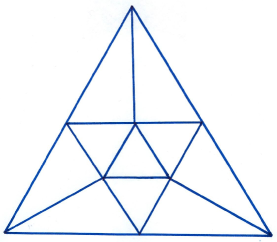
Figure 2. Dranishnikov subdivision of triangles.

1. each tetrahedron in $N_{i}$ that was a join of an interior vertex with a triangle $\sigma\subset\partial N_{i}$ gets replaced by the join of the same vertex with $\sigma^{*}$ (i.e. we cone the subdivision of $\sigma$ to the interior vertex), subdividing the original tetrahedron into ten new tetrahedra (the cone over Figure 2), and

2. each tetrahedron that was a join of an edge on the square with an edge on $\partial N_{i}$ gets replaced by two tetrahedra (i.e. the join of the internal edge with each of the two edges obtained from subdividing the boundary edge).

This changes the original triangulation on each $N_{i}$ into a new triangulation $N_{i}^{\prime}$ with a total of $264$ tetrahedrons. We will continue to use the term block to refer to the subcomplexes of the $N_{i}^{\prime}$ that are subdivisions of the original blocks in $N_{i}$. Observe that, in each of the $N_{i}$, our subdivision process did not introduce any new vertices in the interior of the $N_{i}$. As such, the core squares have been left unchanged (and we will still refer to them as the cores of the $N_{i}^{\prime}$).

Finally, we note that by construction the two subdivisions $N_{i}^{\prime}$ of $N_{i}$, and $X^{*}$ of $X$ coincide on their common subcomplex $\partial N_{i}=N_{i}\cap X$. In particular, they glue together to give a well defined triangulation $\Sigma$ of $S^{3}$.

Step 4: Verifying that $\Sigma$ has the desired properties.

Note that the triangulation $\Sigma$ contains a copy of $X^{*}$, as well as copies of each $N_{i}^{\prime}$. These partition the triangulation $\Sigma$ into various pieces.

Lemma 4.

The complex $X^{*}$, the individual $N_{i}^{\prime}$, and the intersections $X^{*}\cap N_{i}^{\prime}$, are all full subcomplexes of $\Sigma$.

Proof.

This follows easily from the following two facts:

• each of the intersections $X^{*}\cap N_{i}^{\prime}=(X\cap N_{i})^{*}$ is a full subcomplex of $X^{*}$,

• each of the intersections $X^{*}\cap N_{i}^{\prime}=\partial N_{i}^{\prime}$ is a full subcomplex of the corresponding $N_{i}^{\prime}$.

The first statement is a direct consequence of [PS, Lemma 2.10], where it is shown that if $U$ is any subcomplex of $W$, then $U^{*}$ is a full subcomplex of $W^{*}$. The second statement is a consequence of the construction of the triangulation $N_{i}^{\prime}$, since by construction, each simplex of $N_{i}^{\prime}$ which is not contained in $\partial N_{i}^{\prime}$ contains a vertex in the interior of $N_{i}^{\prime}$ (and hence in $N_{i}^{\prime}-\partial N_{i}^{\prime}$). ∎

Lemma 5.

The triangulation $N_{i}^{\prime}$ is flag.

Proof.

Given a collection of pairwise incident vertices $V$, there are three possibilities: $V$ contains either two, one, or no interior vertices of $N_{i}^{\prime}$. We consider each of these three cases in turn.

If $V$ contains no interior vertices, then $V\subset\partial N_{i}^{\prime}$, and since the latter is a full subcomplex of $N_{i}^{\prime}$ (see Lemma 4), $V$ is in fact a collection of vertices in $\partial N_{i}^{\prime}$ which are pairwise adjacent within $\partial N_{i}^{\prime}$. But recall that $\partial N_{i}^{\prime}$ is just the triangulation $(\partial N_{i})^{*}$, hence is flag. This implies that $V$ spans out a simplex in $\partial N_{i}^{\prime}$.

If $V$ contains one interior vertex $v$, then, by the previous argument, $V-\{v\}$ spans a simplex in $\partial N_{i}^{\prime}=(\partial N_{i})^{*}$ which is contained within some (maximal) 2-dimensional simplex $\sigma$ in $(\partial N_{i})^{*}$. Note that, since all vertices $V-\{v\}$ are adjacent to the interior vertex $v$, they must lie in the block $B$ corresponding to $v$. So the 2-dimensional simplex $\sigma\subset(\partial N_{i})^{*}$ can additionally be chosen to lie within that same block $B$. This means that there exists a 2-dimensional simplex $\tau\in\partial N_{i}$ with the property that $\sigma$ is one of the 10 triangles in $\tau^{*}$ (see Figure 2). Finally, observe $\tau$ must lie within the block $B$, so the join of $\tau$ with the interior vertex $v$ defines a tetrahedron inside the original triangulation $N_{i}$ (of type (a) in the terminology of Step 3). But recall how the subdivision $(\partial N_{i})^{*}$ of the triangulation $\partial N_{i}$ was extended into $N_{i}$: for tetrahedra of type (a), the subdivision on the boundary was coned off to the interior vertex. This implies that the join of $\sigma$ and the vertex $v$ defines a tetrahedron in $N_{i}^{\prime}$, and as the set $V$ is a subset of the vertex set of this tetrahedron, we deduce that $V$ spans a simplex in $N_{i}^{\prime}$.

Finally, if $V$ contains two interior vertices $v,w$, let $B_{v},B_{w}$ denote the corresponding blocks. Since $V-\{v,w\}$ is a collection of vertices in $\partial N_{i}^{\prime}=(\partial N_{i})^{*}$ which are adjacent to both interior vertices, we see that the set $V-\{v,w\}$ must lie within $B_{v}\cap B_{w}$, which is a 1-dimensional complex homeomorphic to $S^{1}$ (subdivided into 6 consecutive edges). Since $V-\{v,w\}$ are pairwise adjacent, there is an edge $\sigma$ in $B_{v}\cap B_{w}$ whose vertex set contains $V-\{v,w\}$. This edge is contained in a subdivision of an edge $\tau$ from the original triangulation $\partial N_{i}$, where $\tau$ is an edge which is common to the two blocks $B_{v}$ and $B_{w}$. In particular, the join $\omega*\tau$ of $\tau$ with the edge $\omega$ in the core joining $v$ to $w$ defines a tetrahedron in the original triangulation $N_{i}$ (of type (b) in the terminology of Step 3). Again, from the way the subdivision $(\partial N_{i})^{*}$ was extended inwards, we recall that the tetrahedra $\omega*\tau$, being of type (b), gets replaced by two tetrahedra $\omega*\sigma$ and $\omega*\sigma^{\prime}$, where $\tau^{*}=\sigma\cup\sigma^{\prime}$. Since the join of $\sigma$ and $\omega$ defines a tetrahedron in $N_{i}^{\prime}$, and the set $V$ is a subset of the vertex set of this tetrahedron, we again deduce that $V$ spans a simplex in $N_{i}^{\prime}$. ∎

Corollary 6.

The triangulation $\Sigma$ is flag.

Proof.

If all of the vertices are contained in $X^{*}$, then the claim follows immediately from the fact that $X^{*}$ itself is flag (see [PS, Proposition 2.13]). So we can now assume that at least one of the vertices is contained in the interior of one of the $N_{i}^{\prime}$.

Note that an interior vertex in one of the $N_{i}^{\prime}$ has its closed star entirely contained within the same $N_{i}^{\prime}$. So we see that the tuple of pairwise adjacent vertices must be entirely contained within the same subcomplex $N_{i}^{\prime}$. But by Lemma 5, we have that each of the subdivided $N_{i}^{\prime}$ are themselves flag, finishing the proof. ∎

Proposition 7.

The only squares in $\Sigma$ are the cores of the various $N_{i}^{\prime}$.

Proof.

To see this, let us start with an arbitrary square $(v_{1},v_{2},v_{3},v_{4})$ inside the triangulation $\Sigma$. Our goal is to show that all four vertices must be interior vertices to a single $N_{i}^{\prime}$, which would then force the square to be the core of the corresponding $N_{i}^{\prime}$. To this end, we first note that, if the square does not contain any interior vertex to any of the $N_{i}^{\prime}$, then it is contained entirely within $X^{*}$. But from Lemma 4, the latter is a full subcomplex of $\Sigma$, and by the result of Przytycki and Świ ‘ a tkowski [PS, Proposition 2.13], has no squares. So we may assume that at least one of the vertices is an interior vertex to some $N_{i}^{\prime}$.

If all the vertices are interior to $N_{i}^{\prime}$, then we are done, so by way of contradiction we can also assume that the square contains a vertex which is not interior to $N_{i}^{\prime}$ (which we will call exterior vertices to $N_{i}^{\prime}$). Now the square $(v_{1},v_{2},v_{3},v_{4})$ contains exactly four edges, and since it contains vertices which are both interior and exterior to $N_{i}^{\prime}$, we must have that at least two of the four edges must connect an interior vertex to an exterior vertex (call these intermediate edges).

We now argue that in fact the square must contain exactly two intermediate edges. Indeed, if there were $\geq 3$ intermediate edges, then one could find a pair of adjacent intermediate edges, which share a common exterior vertex. Up to cyclic relabeling, we may assume that $v_{1}$ is the exterior vertex. Considering the other endpoints of these two intermediate edges, we see that $v_{2},v_{4}$ are interior vertices for $N_{i}^{\prime}$, which are both adjacent to the exterior vertex $v_{1}\in\partial N_{i}^{\prime}$. But this implies that the two blocks whose bottoms contain $v_{2}$ and $v_{4}$ cannot be opposite, so must in fact be adjacent. This forces $v_{2}$ and $v_{4}$ to be adjacent vertices in the core of $N_{i}^{\prime}$, contradicting the fact that $(v_{1},v_{2},v_{3},v_{4})$ forms a square. So our hypothetical square $(v_{1},v_{2},v_{3},v_{4})$ must have exactly two intermediate edges, leaving us with exactly two possibilities:

1. the intermediate edges are not adjacent in the square $(v_{1},v_{2},v_{3},v_{4})$,

2. the intermediate edges are adjacent at an interior vertex of $N_{i}^{\prime}$, and the remaining edges are exterior.

We now explain why each of these possibilities give rise to a contradiction.

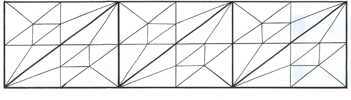
Figure 3. Triangulation on the boundary of a block.

In case (1), we note that up to cyclic relabeling, we have that $v_{1},v_{2}$ are adjacent vertices in the core of the $N_{i}^{\prime}$, while $v_{3},v_{4}$ are adjacent vertices in $\partial N_{i}^{\prime}$. We can also assume that the top of the block $B_{1}$ corresponding to $v_{1}$ attaches to the bottom of the block $B_{2}$ corresponding to $v_{2}$. Now recall that an interior vertex is only adjacent to boundary vertices in its corresponding block. Since $v_{3}$ is adjacent to $v_{2}$, we have that $v_{3}$ must lie in the block $B_{2}$. Similarly, the vertex $v_{4}$ being adjacent to $v_{1}$ must lie in the block $B_{1}$. Since $v_{3}$ and $v_{4}$ are adjacent, we conclude that one of these two vertices must lie in the common boundary $B_{1}\cap B_{2}$. But such a vertex is incident to both $v_{1}$ and $v_{2}$, violating the square condition for $(v_{1},v_{2},v_{3},v_{4})$.

It remains to rule out case (2). To this end, we may again assume that $v_{1}$ is the common interior vertex for the two intermediate edges. Now if $B$ denotes the block corresponding to $v_{1}$, then we have that the boundary vertices $v_{2},v_{4}$, both being adjacent to $v_{1}$, must actually lie in $B$. Moreover, for $(v_{1},v_{2},v_{3},v_{4})$ to be a square, we must have that $v_{3}$ is not adjacent to $v_{1}$, and hence $v_{3}\notin B$. Since $v_{3}$ is adjacent to both the vertices $v_{2},v_{4}\in B$, we see that the latter are either both in the top of $B$ or both in the bottom of $B$, while $v_{3}$ lies in an adjacent block $B^{\prime}$. Let us assume that the vertices lie in the top of $B$ (the other case being completely analogous), so that we can view $v_{2},v_{4}$ as lying in the bottom of the block $B^{\prime}$.

We now have the following situation occurring inside the boundary of the block $B^{\prime}$: we have two vertices $v_{2},v_{4}$ lying in the bottom of the block, and we have a vertex $v_{3}$ which does not lie in the bottom of $B^{\prime}$, but which is adjacent to both $v_{2}$ and $v_{4}$. Now recall that the triangulation of the block $B^{\prime}$ is a subdivision (given in Step 3) of a canonical triangulation of the triangular prism. This subdivision takes the boundary of the original triangulation and applies the Dranishnikov subdivision procedure to it: each edge gets subdivided into two, and each triangle gets replaced by the subdivision in Figure 2. The resulting triangulation on $S^{1}\times[0,1]$ is shown in Figure 3. In the illustration, the left and right side of the rectangle have to be identified, and the “bottom” and “top” of the boundary of the block is precisely the bottom and the top of the rectangle. Note that this triangulation actually consists of six original triangles (see Step 1), each of which has been subdivided into 10 triangles as in Figure 2 (see Step 3). Finally, inspecting the triangulation in Figure 3, we observe that there are exactly six vertices which are adjacent to two distinct vertices in the bottom of the block: these are the only possibilities for $v_{3}$. But for each of these six vertices, we see that the two adjacent vertices in the bottom of the block (i.e. the corresponding $v_{2}$ and $v_{4}$) are adjacent to each other, contradicting the fact that $(v_{1},v_{2},v_{3},v_{4})$ was a square.

Since we’ve ruled out all other possibilities, we see that the square cannot contain any intermediate edges, i.e. the four vertices of our hypothetical square $(v_{1},v_{2},v_{3},v_{4})$ must all lie in the interior of a single $N_{i}^{\prime}$. This implies that our square must coincide with the core of one of the $N_{i}^{\prime}$, as desired.

∎

It follows from Corollary 6 that the triangulation $\Sigma$ is flag, and from Proposition 7 that it has isolated squares with type given by the original link $k$. This completes the proof of Theorem 3.

4. Constructing the manifold.

In this section, we establish the Main Theorem. Our goal is to use some of the triangulations of $S^{3}$ constructed in the previous section to produce a 4-dimensional manifold $M$ with the desired properties. In order to do this, we start by reviewing some properties of the Davis complex for right angled Coxeter groups.

Recall that one can associate to the 1-skeleton of any simplicial complex $L$ a corresponding right angled Coxeter group $\Gamma_{L}$. This group has one generator $x_{i}$ of order two for each vertex $v_{i}$ of the simplicial complex $L$, and a relation $x_{i}x_{j}=x_{j}x_{i}$ whenever the corresponding vertices $v_{i},v_{j}$ are adjacent in $L$. Let us consider the associated Davis complex $\tilde{P}_{L}$. This complex is obtained via the following procedure: we first consider the cubical complex $[-1,1]^{V(L)}$, that is to say, the standard cube with dimension equaling the number of vertices in the simplicial complex $L$. Now every face of the cube is an affine translation of $[-1,1]^{S}$ for some subset $S\subset V(L)$, which we call the type of the face. Consider the cubical subcomplex $P_{L}\subset[-1,1]^{V(L)}$ consisting of all faces whose type defines a simplex in $L$, and let $\tilde{P}_{L}$ to be its universal cover. Observe that the Coxeter group $\Gamma_{L}$ acts on $P_{L}$, where each generator $x_{i}$ acts by reflection on the corresponding coordinate. The kernel of the resulting morphism $\Gamma_{L}\rightarrow(\mathbb{Z}_{2})^{|V(L)|}$ coincides with the fundamental group of $P_{L}$. There is a natural piecewise flat metric on $P_{L}$, obtained by making each $k$-dimensional face in the cubulation of $P_{L}$ isometric to $[-1,1]^{k}\subset\mathbb{R}^{k}$. Properties of the cubical complex $P_{L}$ are intimately related to properties of the simplicial complex $L$. For instance, we have:

1. if $L$ is a flag complex, then the piecewise flat metric on $P_{L}$ is locally CAT(0),

2. the links of vertices in $P_{L}$ are canonically simplicially isomorphic to $L$,

3. if $L$ is the join of two subcomplexes $L_{1},L_{2}$, then the space $P_{L}$ splits isometrically as a product of $P_{L_{1}}$ and $P_{L_{2}}$,

4. if $L^{\prime}$ is a full subcomplex of $L$, then the natural inclusion induces a totally geodesic embedding $P_{L^{\prime}}\hookrightarrow P_{L}$,

5. if the geometric realization of $L$ is homeomorphic to an $(n-1)$-dimensional sphere, then $P_{L}$ is an $n$-dimensional manifold,

6. if $L$ is a PL-triangulation of $S^{n-1}$ then $P_{L}$ is a PL-manifold, and $\partial^{\infty}\tilde{P}_{L}$ is homeomorphic to $S^{n-1}$,

7. if $L$ is a smooth triangulation of $S^{n-1}$, then $P_{L}$ is a smooth manifold.

These results are discussed in detail in the book [Da1].

In the previous section, we showed that given a prescribed link $k$ in $S^{3}$, one can construct a triangulation of $S^{3}$ with isolated squares, and with type the given link. Let us apply this result in the special case where $k$ is a nontrivial knot inside $S^{3}$. Let $L$ denote the corresponding triangulation of $S^{3}$. Since we are in the special case of dimension $=3$, the triangulation $L$, in addition to being flag, is automatically PL and smooth. We now consider the cubical complex $M:=P_{L}$ associated to the corresponding right angled Coxeter group $\Gamma_{L}$. In view of our earlier discussion, we have the following:

Fact 1: The space $M$ is a smooth 4-manifold (from (g) above), and the natural piecewise Euclidean metric on $M$ induced from the cubulation is locally CAT(0) (from (a) above). Furthermore, the boundary at infinity of $\tilde{M}$ is homeomorphic to $S^{3}$ (from (f) above), and $\tilde{M}$ is diffeomorphic to $\mathbb{R}^{4}$.

The very last statement in Fact 1 can be deduced from work of Stone (see [St, Theorem 1]), who showed that a metric (piecewise flat) polyhedral complex which is both CAT(0) and a PL-manifold without boundary must in fact be PL-homeomorphic to the appropriate $\mathbb{R}^{n}$. Since our $\tilde{M}$ satisfies these conditions, this ensures that $\tilde{M}$ is PL-homeomorphic to the standard $\mathbb{R}^{4}$. But in the 4-dimensional setting, there is no difference between PL and smooth, so $\tilde{M}$ is in fact diffeomorphic to $\mathbb{R}^{4}$.

Our goal is now to show that $M$ has the properties postulated in our Main Theorem. Note that properties (1) and (2) are included in Fact 1, while property (4) can be easily deduced from property (3) (see the comment after the proof of Proposition 1). So we are left with establishing property (3): that $\pi_{1}(M)$ cannot be isomorphic to the fundamental group of any nonpositively curved Riemannian manifold. This last property will be established by looking at the large scale geometry of flats inside the universal cover $\tilde{M}$.

As a starting point, let us describe some flats inside $\tilde{M}$. Observe that each square inside the triangulation $L$ is a full subcomplex isomorphic to a 4-cycle $\square$. The right angled Coxeter group associated to a 4-cycle is a direct product of two infinite dihedral groups $\Gamma_{\square}\cong D_{\infty}\times D_{\infty}=(\mathbb{Z}_{2}*\mathbb{Z}_{2})\times(\mathbb{Z}_{2}*\mathbb{Z}_{2})$ (see (c) above). The corresponding complex $P_{\square}$ is isometric to a flat torus (with cubulation given by 16 squares, obtained via the identification $S^{1}\times S^{1}=\square\times\square$). By considering the unique square inside the triangulation $L$, we obtain:

Fact 2: $M$ contains a totally geodesic $2$-dimensional flat torus $T^{2}$ (see (d) above). Furthermore, at any vertex $v\in T^{2}\subset M$ of the cubulation, we have that the torus $T^{2}$ is locally knotted inside the ambient $4$-dimensional manifold $M$ (see (b) above), in that there is a canonical simplicial isomorphism $\big{(}lk_{v}(M),lk_{v}(T^{2})\big{)}\cong(L,k)$ where $k$ is the unique (knotted) square in the triangulation $L$.

Since the embedding $T^{2}\hookrightarrow M$ is totally geodesic, by lifting to the universal cover, we obtain a $2$-dimensional flat $F\hookrightarrow\tilde{M}$ which is locally knotted at lifts of vertices. This induces an embedding of the corresponding boundaries at infinity, giving us an embedding of $\partial^{\infty}F\cong S^{1}$ into $\partial^{\infty}\tilde{M}\cong S^{3}$. The rest of our argument will rely on the following “local-to-global” assertion:

Assertion: The embedding $\partial^{\infty}F\cong S^{1}$ into $\partial^{\infty}\tilde{M}\cong S^{3}$ defines a nontrivial knot in the boundary at infinity of $\tilde{M}$.

That is to say, the “local knottedness” of the flat propagates to “global knottedness” of its boundary at infinity. For the sake of exposition, we delay the proof of the assertion, and first show how we can use it to deduce the Main Theorem. To this end, let us assume that $(M^{\prime},g)$ is a closed manifold equipped with a Riemannian metric of nonpositive sectional curvature, and that we are given an isomorphism of fundamental groups $\phi:\Gamma=\pi_{1}(M)\rightarrow\pi_{1}(M^{\prime})$. From this assumption, we want to work towards a contradiction.

The first step is to use the isomorphism of fundamental groups to obtain an equivariant homeomorphism between the corresponding boundaries at infinity. As a cautionary remark, we recall that given a pair $X_{1},X_{2}$ of CAT(0)-spaces with geometric $G$-actions, a celebrated example of Croke and Kleiner [CK] shows that the corresponding boundaries at infinity $\partial^{\infty}X_{1}$ and $\partial^{\infty}X_{2}$ need not be homeomorphic. Even if the boundaries at infinity are homeomorphic, an example of Buyalo [Bu] shows that the homeomorphism might not be equivariant with respect to the $G$-action.

In his thesis [H], Hruska introduced CAT(0)-spaces with isolated flats. Subsequent work of Hruska and Kleiner [HK] established the following two foundational results for CAT(0)-spaces with isolated flats:

1. for a pair $X_{1},X_{2}$ of CAT(0)-spaces with geometric $G$-actions, if $X_{1}$ has isolated flats, then so does $X_{2}$ (see [HK, Corollary 4.1.3]), and there is a $G$-equivariant homeomorphism between $\partial^{\infty}X_{1}$ and $\partial^{\infty}X_{2}$ (see [HK, Theorem 4.1.8]).

2. for a group $G$ acting geometrically on a CAT(0)-space $X$, we have that $X$ has the isolated flats property if and only if $G$ is a relatively hyperbolic group with respect to a collection of virtually abelian subgroups of rank $\geq 2$ (see [HK, Theorem 1.2.1]).

As such, if we could establish that our group $\Gamma$ is a relatively hyperbolic group with respect to a collection of virtually abelian subgroups of rank $\geq 2$, then result (2) above would ensure that our CAT(0)-manifold $\tilde{M}$ has the isolated flats property. Result (1) above would then give the desired $\Gamma$-equivariant homeomorphism between $\partial^{\infty}\tilde{M}$ and $\partial^{\infty}\tilde{M}^{\prime}$. So our next goal is to establish:

Fact 3: The group $\Gamma=\pi_{1}(M)$ is hyperbolic relative to the collection of all virtually abelian subgroups of $\Gamma$ of rank $\geq 2$.

The notion of a group $G$ being relatively hyperbolic with respect to a collection $\mathcal{A}$ of subgroups of $G$ was originally suggested by Gromov [Gr], whose approach was later formalized by Bowditch [Bo]. Alternate formulations appear in Farb’s thesis [Fa], in work of Druţu and Sapir [DrSa], and in the memoir of Osin [Os]. We refer the reader to the original sources for a detailed definition as well as basic properties of such groups. For our purposes, we merely need to know that the property of a group $G$ being hyperbolic relative to a collection of virtually abelian subgroups of rank $\geq 2$ is inherited by finite index subgroups of $G$. In particular, to show the desired property for $\Gamma$, we see that it is sufficient to establish that our original Coxeter group $\Gamma_{L}$ is relatively hyperbolic with respect to higher rank virtually abelian subgroups (since $\Gamma\leq\Gamma_{L}$ is of finite index).

Caprace [Ca, Cor. D (ii)] recently provided a criterion for deciding whether a Coxeter group is hyperbolic relative to the collection of its higher rank virtually abelian subgroups. In the right-angled case the condition is that the flag complex $L$ which defines $\Gamma_{L}$ contains no full subcomplex isomorphic to the suspension $\Sigma K$ of a subcomplex $K$ with 3 vertices which is either

1. the disjoint union of 3 points, or

2. the disjoint union of an edge and 1 point.

In both cases $\Sigma K$ does not have isolated squares. Since the Coxeter group $\Gamma_{L}$ with which we are working is associated to a triangulation $L$ of $S^{3}$ with isolated squares, we conclude that $\Gamma_{L}$ is relatively hyperbolic with respect to the collection of all virtually abelian subgroups of rank $\geq 2$. Hence, Fact 3.

Applying Hruska and Kleiner’s results from [HK], we conclude that the original $\tilde{M}$ is a CAT(0)-space with the isolated flats property, and that there exists a $\Gamma$-equivariant homeomorphism from $\partial^{\infty}\tilde{M}$ to $\partial^{\infty}\tilde{M}^{\prime}$. The nontrivial knot $\partial^{\infty}F\cong S^{1}$ inside $\partial^{\infty}\tilde{M}\cong S^{3}$ appearing in the Assertion can be identified with the limit set of the corresponding subgroup $\pi_{1}(T^{2})\cong\mathbb{Z}^{2}\leq\Gamma=\pi_{1}(M)$. Since we have an equivariant homeomorphism between the boundaries at infinity of $\tilde{M}$ and $\tilde{M}^{\prime}$, this immediately yields:

Fact 4: The boundary at infinity $\partial^{\infty}\tilde{M}^{\prime}$ is homeomorphic to $S^{3}$, and the limit set of the canonical $\mathbb{Z}^{2}$-subgroup in $\Gamma\cong\pi_{1}(M^{\prime})$ defines a nontrivial knot $S^{1}\hookrightarrow\partial^{\infty}\tilde{M}^{\prime}\cong S^{3}$.

On the other hand, the flat torus theorem implies that there exists a $\mathbb{Z}^{2}$-periodic flat $F^{\prime}\hookrightarrow\tilde{M}^{\prime}$, with the property that $\partial^{\infty}F^{\prime}$ coincides with the limit set of the $\mathbb{Z}^{2}$. In particular, $\partial^{\infty}F^{\prime}$ defines a nontrivial knot inside $\partial^{\infty}M^{\prime}$. But taking any point $p\in F^{\prime}$, we note that geodesic retraction provides a homeomorphism $\rho:\partial^{\infty}\tilde{M}^{\prime}\rightarrow T_{p}\tilde{M}^{\prime}$. This homeomorphism takes the knotted subset $\partial^{\infty}F^{\prime}$ lying inside $S^{3}\cong\partial^{\infty}M^{\prime}$ to the unknotted subset $T_{p}F^{\prime}$ lying inside $S^{3}\cong T_{p}\tilde{M}^{\prime}$. This contradiction allows us to conclude that no such Riemannian manifold $(M^{\prime},g)$ can exist.

So in order to complete the proof of the Main Theorem, we are left with establishing the Assertion. We note that a similar result was shown in the setting of CAT(-1)-manifolds by Farrell and Lafont [FL], the proof of which extends almost verbatim to yield the Assertion. For the convenience of the reader, we provide a (slightly different) self-contained argument for the Assertion.

The basic idea is as follows: picking a vertex $v\in F$, we have a geodesic retraction map $\rho:\partial^{\infty}\tilde{M}\rightarrow lk_{v}(\tilde{M})$. Under this map, we see that $\partial^{\infty}F$ maps to the link $lk_{v}(F)$ inside $lk_{v}(\tilde{M})$. But recall from Fact 2 that the torus is locally knotted in $\tilde{M}$, i.e. the pair $\big{(}lk_{v}(\tilde{M}),lk_{v}(F)\big{)}$ is simplicially isomorphic to $(S^{3},k)$, where $S^{3}$ is the 3-sphere equipped with the triangulation $L$, and $k$ is the knot in $S^{3}$ given by the unique square in the triangulation $L$. Now the retraction map $\rho$ is not a homeomorphism, but is nevertheless “close enough” to a homeomorphism for us to use it to compare the pair $\big{(}\partial^{\infty}\tilde{M},\partial^{\infty}F\big{)}$ with the knotted pair $\big{(}lk_{v}(\tilde{M}),lk_{v}(F)\big{)}\cong(S^{3},k)$. More precisely, for any given subset $Z\subset lk_{v}(\tilde{M})\cong S^{3}$ we denote by $Z_{\infty}$ the corresponding pre-image $Z_{\infty}:=\rho^{-1}(Z)$ inside $\partial^{\infty}\tilde{M}$. Then we have:

Fact 5: [FL, Proposition 2, pg. 627] For any open set $U\subset lk_{v}(\tilde{M})$, the map $\rho:U_{\infty}\rightarrow U$ is a proper homotopy equivalence. Moreover, the map $\rho$ is a near-homeomorphism, i.e. can be approximated arbitrarily closely by homeomorphisms.

This is shown by identifying $U_{\infty}$ with the inverse limit of the sets $\{U_{r}\}_{r\in\mathbb{R}^{+}}$, where each $U_{r}$ is the pre-image of $U$ under the geodesic projection from the sphere $S_{v}(r)$ of radius $r$ centered at $v$ to the link at $v$. For $r>s$, the bonding maps $\rho_{r,s}:U_{r}\rightarrow U_{s}$ are given by geodesic retraction, and the canonical map $\rho_{\infty,s}$ from $U_{\infty}=\varprojlim\{U_{r}\}$ to each individual $U_{s}$ coincides with the geodesic retraction map. Since the link $lk_{v}(\tilde{M})$ can be identified with $S_{\epsilon}(r)$, a small enough $\epsilon$-sphere centered at $v$, the map $\rho$ can be identified with the canonical map $\rho_{\infty,\epsilon}$ from $U_{\infty}=\varprojlim\{U_{r}\}$ to the corresponding $U_{\epsilon}=U$. Now by results of Davis and Januszkiewicz [DJ, Section 3] each of the bonding maps $\rho_{r,s}$ are cell-like maps, i.e. point pre-images have the shape of a point (see Dydak and Segal [DySe] for background on shape theory). Since the shape functor commutes with inverse limits, and since $\rho=\rho_{\infty,\epsilon}$, we see that $\rho$ is also a cell-like map. A result of Edwards [Ed, Section 4] now implies that $\rho$ is a proper homotopy equivalence, while work of Armentrout [Ar] ensures that $\rho$ is a near homeomorphism.

Now to show that $\partial^{\infty}F$ defines a nontrivial knot in $\partial^{\infty}\tilde{M}$, we need to establish that the complement $\partial^{\infty}\tilde{M}-\partial^{\infty}F$ cannot be homeomorphic to $S^{1}\times\mathbb{R}^{2}$. This will follow if we can show that $\pi_{1}\big{(}\partial^{\infty}\tilde{M}-\partial^{\infty}F\big{)}$ is a non-abelian group. To do this, let us decompose $\partial^{\infty}\tilde{M}-\partial^{\infty}F$ into a union of a suitable pair of open sets. We start by decomposing $lk_{v}(\tilde{M})$, and will then use the map $\rho$ to “lift” this decomposition to $\partial^{\infty}\tilde{M}$. Let $lk_{v}(F)\subset N_{1}\subset N_{2}\subset lk_{v}(\tilde{M})$ be nested open regular neighborhoods of the knot $k=lk_{v}(F)$ inside $S^{3}\cong lk_{v}(\tilde{M})$. Define open sets in $lk_{v}(\tilde{M})$ by setting $U_{2}:=N_{2}$, and $U_{1}:=lk_{v}(\tilde{M})-\bar{N}_{1}$, where $\bar{N}_{1}$ denotes the closure of $N_{1}$. Note that we have homeomorphisms $U_{2}\cong S_{1}\times\mathbb{D}^{2}$ and $U_{1}\cap U_{2}\cong N_{2}-\bar{N}_{1}\cong S^{1}\times S^{1}\times\mathbb{R}$, while $U_{1}$ is homeomorphic to the complement of the nontrivial knot $k\subset S^{3}$. So at the level of $\pi_{1}$, we have that (a) $\pi_{1}(U_{1}\cap U_{2})\cong\mathbb{Z}\oplus\mathbb{Z}$, and (b) $\pi_{1}(U_{1})$ is a non-abelian group. The latter fact follows from work of Papakyriakopoulos [Pa], who showed that $\pi_{1}$ of the complement of a nontrivial knot cannot be isomorphic to $\mathbb{Z}$. But by Alexander duality such a group must have abelianization isomorphic to $\mathbb{Z}$, hence cannot be abelian.

Now corresponding to this decomposition of $lk_{v}(\tilde{M})$, we have an associated open decomposition of $\partial^{\infty}\tilde{M}$ in terms of the corresponding $(U_{1})_{\infty}$, $(U_{2})_{\infty}$. We now define an open decomposition of $\partial^{\infty}\tilde{M}-\partial^{\infty}F$ by setting $U:=(U_{1})_{\infty}$ and $V:=(U_{2})_{\infty}-\partial^{\infty}F$. The intersection satisfies $U\cap V=(U_{1}\cap U_{2})_{\infty}$. Applying Fact 5 to the discussion in the previous paragraph, we obtain that (a) $\pi_{1}(U\cap V)\cong\mathbb{Z}\oplus\mathbb{Z}$, and (b) $\pi_{1}(U)$ is non-abelian. From Seifert-Van Kampen, we have:

$$\pi_{1}\big{(}\partial^{\infty}\tilde{M}-\partial^{\infty}F\big{)}=\pi_{1}(U)*_{\pi_{1}(U\cap V)}\pi_{1}(V)$$

So to see that $\pi_{1}\big{(}\partial^{\infty}\tilde{M}-\partial^{\infty}F\big{)}$ is non-abelian, it suffices to show that the non-abelian group $\pi_{1}(U)$ injects into the amalgamation. But this will follow from:

Fact 6: The map $i_{*}:\pi_{1}(U\cap V)\rightarrow\pi_{1}(V)$ induced by inclusion is injective.

To establish Fact 6, we first choose a suitable basis for $\pi_{1}(U\cap V)\cong\mathbb{Z}\oplus\mathbb{Z}$. Recall that the map $\rho$ gives a proper homotopy equivalence between $U\cap V=(U_{1}\cap U_{2})_{\infty}$ and the space $U_{1}\cap U_{2}=N_{2}-\bar{N}_{1}$, where $N_{1}\subset N_{2}$ are nested open regular neighborhoods of the knot $k$. Since $U_{2}=N_{2}$ can be identified with $S^{1}\times\mathbb{D}^{2}$, where $S^{1}\times\{0\}$ corresponds to the knot $k$, we choose the generators for $\pi_{1}(N_{2}-\bar{N}_{1})\cong\mathbb{Z}\oplus\mathbb{Z}$ to have the following two properties:

1. the generator $\langle 1,0\rangle$ maps to a generator represented by $[S^{1}\times\{0\}]\in\pi_{1}(N_{2})\cong\mathbb{Z}$ under the obvious inclusion, and

2. the generator $\langle 0,1\rangle$ is chosen so that a representative curve exists which, under the natural inclusion into $N_{2}\cong S^{1}\times\mathbb{D}^{2}$, projects to a generator for $\pi_{1}(\mathbb{D}^{2}-\{0\})\cong\mathbb{Z}$ in the $\mathbb{D}^{2}$-factor, and is null-homotopic in $N_{2}$.

We choose the generators of $\pi_{1}(U\cap V)\cong\mathbb{Z}\oplus\mathbb{Z}$ to map to the above two generators of $\pi_{1}(U_{1}\cap U_{2})$ under the homotopy equivalence $\rho$.

To verify that $i_{*}:\pi_{1}(U\cap V)\rightarrow\pi_{1}(V)$ is injective, we first argue that an element $\langle a,b\rangle\in\ker(i_{*})$ must satisfy $a=0$. Consider the commutative diagram:

where all horizontal arrows are induced by the obvious inclusions, and the two vertical arrows are the isomorphisms induced by the geodesic retraction maps. By the choice of the basis on $\pi_{1}(U\cap V)$, we have that $\rho_{*}(\langle a,b\rangle)=\langle a,b\rangle\in\pi_{1}(U_{1}\cap U_{2})$, which by property (A) maps to $a\in\mathbb{Z}\cong\pi_{1}(N_{2})$. From the commutativity of the diagram, we conclude that if $\langle a,b\rangle\in\ker(i_{*})$, then $a=0$. Our next goal is to show that $b=0$.

Given a pair $\eta_{1},\eta_{2}$ of disjoint oriented curves in $S^{1}\times\mathbb{D}^{2}$, with $\eta_{1}$ null-homotopic, there is a well-defined linking number $L(\eta_{1},\eta_{2})$. For smooth curves this is obtained by looking at the oriented intersection number of $\eta_{2}$ with a smooth bounding disk for the curve $\eta_{1}$, and for continuous curves one uses an approximation by smooth curves. This linking number has the property that if $\eta_{1}\sim\eta_{1}^{\prime}$ (respectively $\eta_{2}\sim\eta_{2}^{\prime}$) are two curves homotopic to each other in the complement of $\eta_{2}$ (respectively $\eta_{1}$), then $L(\eta_{1},\eta_{2}^{\prime})=L(\eta_{1},\eta_{2})=L(\eta_{1}^{\prime},\eta_{2})$.

Now from the choice of basis on $\pi_{1}(U\cap V)$, along with property (B), we can choose a representative curve $\gamma$ for the element $\langle 0,b\rangle\in\ker(i_{*})\subset\pi_{1}(U\cap V)$ with the property that the image curve $\rho(\gamma)\subset U_{1}\cap U_{2}\subset N_{2}\cong S^{1}\times\mathbb{D}^{2}$ projects to $b$ times a generator for $\pi_{1}(\mathbb{D}^{2}-\{0\})$. One can easily check that this forces $L\big{(}\rho(\gamma),S^{1}\times\{0\}\big{)}=\pm b$. Applying Fact 5, we can find a homeomorphism $\rho^{\prime}:(N_{2})_{\infty}\rightarrow N_{2}$ which is $\epsilon$-close to the map $\rho$. In view of the discussion above, and recalling that the curve $S^{1}\times\{0\}$ corresponds to $lk_{v}(F)=\rho(\partial^{\infty}F)$, this gives us that:

$$\pm b = L\big{(}\rho(\gamma),S^{1}\times\{0\}\big{)}=L\big{(}\rho(\gamma),\rho(\partial^{\infty}F)\big{)}$$

$$= L\big{(}\rho^{\prime}(\gamma),\rho(\partial^{\infty}F)\big{)}=L\big{(}\rho^{\prime}(\gamma),\rho^{\prime}(\partial^{\infty}F)\big{)}=L\big{(}\gamma,\partial^{\infty}F\big{)}$$

where for the last equality, we use the fact that $\rho^{\prime}$ is a homeomorphism, and hence preserves the linking number. But since $\langle 0,b\rangle\in\ker(i_{*})$, we also have that $\gamma$ bounds a disk in $V=(N_{2})_{\infty}-\partial^{\infty}F$, which implies that $L\big{(}\gamma,\partial^{\infty}F\big{)}=0$. This now forces $b=0$, completing the proof of Fact 6.

Since the non-abelian group $\pi_{1}(U)$ injects into $\pi_{1}\big{(}\partial^{\infty}\tilde{M}-\partial^{\infty}F\big{)}$, we obtain that $\partial^{\infty}F\cong S^{1}$ defines a nontrivial knot in $\partial^{\infty}\tilde{M}\cong S^{3}$, establishing the Assertion, and finishing off the proof of the Main Theorem.

5. Concluding remarks.

Finally, we point out a few interesting questions that come up naturally from this work. As discussed in Section 2.2, locally CAT(0)-manifolds whose universal covers are not diffeomorphic to $\mathbb{R}^{n}$ cannot support a Riemannian smoothing. In dimensions $n\neq 4$, there is no difference between “homeomorphic to $\mathbb{R}^{n}$” and “diffeomorphic to $\mathbb{R}^{n}$”. In contrast, it is known that $\mathbb{R}^{4}$ supports many distinct smooth structures (in fact, continuum many). Moreover, the method used to construct the Davis examples of closed aspherical manifolds whose universal covers are not homeomorphic to $\mathbb{R}^{n}$ requires $n\geq 5$. So one can ask:

Question: Can one find locally CAT(0) closed 4-manifolds $M^{4}$ with the property that their universal covers $\tilde{M}^{4}$ are

1. not homeomorphic to $\mathbb{R}^{4}$?

2. homeomorphic, but not diffeomorphic to $\mathbb{R}^{4}$?

Paul Thurston [Th] proved that $\tilde{M}^{4}$ must be homeomorphic to $\mathbb{R}^{4}$ if it has at least one “tame” point. We remark that the result of Stone [St] tells us that there is no hope of constructing such examples via piecewise flat metric complexes (for their universal covers would then have to be diffeomorphic to the standard $\mathbb{R}^{4}$). Moreover, if one asks instead for aspherical closed $4$-manifolds, we remark that Davis [Da2] has constructed examples where the universal cover is not homeomorphic to $\mathbb{R}^{4}$ (but it is unknown whether those examples support a locally CAT(0)-metric).

Now concerning the dimension restriction in our construction, we note that this was due to the need for finding triangulations of spheres with the property that the associated Davis complex had the isolated flats condition (in order to obtain a well-defined boundary at infinity). The “isolated squares” condition we introduced was designed to ensure that Caprace’s criterion was fulfilled. Attempting to generalize this construction to higher dimensions, the difficulty we run into is that, by work of Januszkiewicz and Świ ‘ a tkowski [JS, Section 2.2] (see also the discussion in [PS, Appendix]), there is no higher-dimensional analogue of the Dranishnikov-Przytycki-Świ ‘ a tkowski procedure for modifying triangulations in order to get rid of squares.

Finally, we remark that our construction relies on the presence of flats with specific large scale behavior in order to obstruct Riemannian smoothings. As such, our methods require the presence of zero curvature. If one desires examples which are strictly negatively curved, we are brought to the following:

Question: Can one construct examples of smooth, locally CAT(-1)-manifolds $M^{n}$ with the property that $\partial^{\infty}\tilde{M}$ is homeomorphic to $S^{n-1}$, but which do not support any Riemannian metric of nonpositive sectional curvature?

References

- [ADG] F.D. Ancel, M.W. Davis and C.R. Guilbault, CAT(0) reflection manifolds, in Geometric Topology (Athens, GA, 1993) AMS/IP Stud. Adv. Math., volume 2, Amer. Math. Soc., Providence, RI 1997, pp. 441–445.
- [Ar] S. Armentrout. Cellular decompositions of -manifolds that yield -manifolds, Mem. of the Amer. Math. Soc. 107. American Mathematical Society, Providence, 1971.
- [BL] A. Bartels and W. Lück. The Borel Conjecture for hyperbolic and CAT(0)-groups. Preprint available on the arXiv:0901.0442
- [BLW] A. Bartels, W. Lück, and S. Weinberger. On hyperbolic groups with spheres as boundaries. Preprint available on the arXiv:0911.3725
- [Bo] B. Bowditch. Relatively hyperbolic groups, Preprint, Univ. Southampton (1999).
- [Bu] S. V. Buyalo. Geodesics in Hadamard spaces, St. Petersburg Math. J. 10 (1999), 293–313.
- [Ca] P.-E. Caprace. Buildings with isolated subspaces and relatively hyperbolic Coxeter groups, Preprint available on the arXiv:math/0703799
- [CD] R. Charney and M. W. Davis. Strict hyperbolization, Topology 34 (1995), 329–350.
- [CK] C. Croke and B. Kleiner. Spaces with nonpositive curvature and their ideal boundaries, Topology 39 (2000), 549–556.
- [Da1] M. W. Davis. The geometry and topology of Coxeter groups, London Mathematical Society Monographs Series, 32. Princeton University Press, 2008.
- [Da2] M. W. Davis. Groups generated by reflections and aspherical manifolds not covered by Euclidean space, Ann. of Math. (2) 117 (1983), 293–324.
- [DH] M. W. Davis and J.-C. Hausmann. Aspherical manifolds without smooth or PL structure, in “Algebraic topology (Arcata, CA, 1986)”, pgs. 135–142, Lecture Notes in Math. 1370. Springer, Berlin, 1989.
- [DJ] M. W. Davis and T. Januszkiewicz. Hyperbolization of polyhedra, J. Diff. Geom. 34 (1991), 347–388.
- [Dr] A. N. Dranishnikov. Boundaries of Coxeter groups and simplicial complexes with given links, J. Pure Appl. Algebra 137 (1999), 139–151.
- [DrSa] C. Druţu and M. Sapir. Tree-graded spaces and asymptotic cones of groups (with an appendix by D. Osin and M. Sapir), Topology 44 (2005), 959–1058.
- [DySe] J. Dydak and J. Segal. Shape theory: an introduction. Springer-Verlag, Berlin, 1978.
- [Ed] R. Edwards. The topology of manifolds and cell-like maps, in “Proceedings of the I.C.M., Helsinki”, pgs. 111–127. Acad. Sci. Fennica, Helsinki, 1980.
- [Fa] B. Farb. Relatively hyperbolic groups, Geom. Funct. Anal. 8 (1998), 810–840.
- [FJ] F. T. Farrell and L. E. Jones. Topological rigidity for compact nonpositively curved manifolds, in “Differential geometry: Riemannian geometry (Los Angeles, CA, 1990),” pgs. 229–274, Proc. Sympos. Pure Math. 54, Part 3. Amer. Math. Soc., Providence, RI, 1993.
- [FL] F. T. Farrell and J.-F. Lafont. Involutions of negatively curved groups with wild boundary behavior, Pure Appl. Math. Q. 5 (2009), 619–640.
- [GW] D. Gromoll and J. A. Wolf. Some relations between the metric structure and the algebraic structure of the fundamental group in manifolds of nonpositive curvature, Bull. Amer. Math. Soc. 77 (1971), 545–552.
- [Gr] M. Gromov. Hyperbolic groups, in “Essays in group theory,” pgs. 75–263. Springer-Verlag, NY, 1987.
- [H] C. Hruska. Geometric invariants of spaces with isolated flats, Topology 44 (2005), 441–458.
- [HK] C. Hruska and B. Kleiner. Hadamard spaces with isolated flats (with an appendix by the authors and M. Hindawi), Geom. Topol. 9 (2005), 1501–1538
-
[JS]
T. Januszkiewicz and J. Świ
tkowski. Hyperbolic Coxeter groups of large dimension, Comment. Math. Helv. 78 (2003), 555–583.‘ a - [LY] H. B. Lawson and S. T. Yau. Compact manifolds of nonpositive curvature, J. Differential Geometry 7 (1972), 211–228.
- [Mi] J. Milnor. On manifolds homeomorphic to the -sphere, Ann. of Math. (2) 64 (1956), 399–405.
- [Os] D. Osin. Relatively hyperbolic groups: intrinsic geometry, algebraic properties, and algorithmic problems, Mem. Amer. Math. Soc. 179 (2006), no. 843.
- [Pa] C. D. Papakyriakopoulos. On Dehn’s Lemma and the asphericity of knots, Ann. Math. 66 (1957), 1–26.
-
[PS]
P. Przytycki and J. Świ
tkowski. Flag-no-square triangulations and Gromov boundaries in dimension 3, Groups Geom. Dyn. 3 (2009), 453–468.‘ a - [Sc] V. Schroeder. A splitting theorem for spaces of nonpositive curvature, Invent. Math. 79 (1985), 323–327.
- [St] D. A. Stone. Geodesics in piecewise linear manifolds, Trans. Amer. Math. Soc. 215 (1976), 1–44.
- [Th] P. Thurston, 4-manifolds possessing a single tame point are Euclidean. (English summary) J. Geom. Anal. 6 (1996), no. 3, 475–494.