Recursive set-membership state estimation for linear non-causal time-variant differential-algebraic equation with continuous time

Abstract

This paper describes a state estimation approach for non-causal time-varying linear descriptor equations with uncertain parameters. The uncertainty in the state equation and in the measurements is supposed to admit a set-membership description. The approach is based on the notion of the linear minimax estimation. Suboptimal minimax state estimation algorithm is introduced for DAEs with non-stationary rectangular matrices. Optimal algorithm is presented for DAEs with special structure of the matrices. A comparison of suboptimal and optimal algorithms is presented for 2D time-varying DAE with a singular matrix pencil.

1 Introduction

Dynamical systems described by coupled differential and algebraic equations (DAEs) arise naturally in many applications. In particular, DAEs occur in econometrics (singular dynamic Leotief systems Luenberger and A. (1977)), modelling of constrained multibody systems Mills (2006), electrical circuit synthesis Reis (2008), bioprocess and chemical engineering Becerra et al. (2001), representing a common modelling tool Mehrmann and Stykel (2005). On can divide contributions to the theory of DAEs into results for casual DAEs and results for non-causal systems. 1.1 Causal DAEs. The solvability theory for finite-dimentional systems with constant coefficients

$$Fx_{t}=Cx+Bf$$ (1)

is based on the reduction of the matrix pencil $sF-C$ to the Kronecker canonical form: if $\mathrm{det}[sF-C]\not\equiv 0$ then for all initial values $x(t_{0})=x_{0}$ there exists a unique solution $x(\cdot)$. Changing the basis in the state space and differentiating exactly $s$ times ($d$ is an index of the pencil $sF-C$), one can reduce (1) to some equivalent Ordinary Differential Equation (ODE), provided $f(\cdot)$ is sufficiently smooth and meets some algebraic constraints. The details of the reduction process are presented in Gantmacher (1960). The index $d$ of the pencil $sF-C$ is said Campbell and Petzold (1983) to be an index of linear DAE (1).

The notion of a Standard Canonical Form (SCF) allows to generalize the index approach on variable coefficients: for instance, in Campbell and Petzold (1983) it was shown that (1) with analitical $F(\cdot)$, $C(\cdot)$ and $B(\cdot)$ is solvable iff (1) can be converted into SCF. In Campbell (1987) it was noted that not all solvable DAEs can be put into SCF and the solvable DAE is equal to some differential-algebraic equation in the canonical form which generalize SCF. In this regard, we say that the DAE is causal if 1) it can be reduced (at least locally in the non-linear case) to normal ODE and 2) if it is solvable for the given intial condition $x_{0}$ and input $f(\cdot)$ then the solution is unique.

The geometry of the reduction procedure for nonlinear causal DAEs $F(x,\dot{x})=0$ was investigeted in Reich (1990); Rabier and Rheinboldt (1994), where the index of DAE was defined as a smallest natural $d$ so that the sequence of the constraint manifolds Reich (1990)

$$M_{k}:=TW_{k-1}\cap M_{k-1},W_{k}=\{x\in\mathbb{R}^{n}:(x,p)\in M_{k}\}$$

with $M_{0}:=\{(x,p):F(x,p)=0\}$ becomes stationary for $k>d$. This coincides with the definition of the index of linear DAE. Solvability of the linear casual DAEs with impulses in the input was addressed in Rabier and Rheinboldt (1996). Further discussion of the linear DAEs solvability theory in finite-dimensions and related topics are presented in Mehrmann and Stykel (2005); Samoilenko et al. (2000).

Basic ideas of the index approach (reduction of the pencil $sF-C$ to the canonical form) were extended on systems with constant operator coefficients in Rutkas (1975), provided the poles of the operator-valued function $s\mapsto(sF-C)^{-1}$ are contained in some bounded vicinity of $0$.

1.2 Non-causal DAEs. The non-causal DAE may have several solutions. For instance, consider

$$\dfrac{d}{dt}\bigl{[}\begin{smallmatrix}1&&0\end{smallmatrix}\bigr{]}(\begin{smallmatrix}x_{1}\\ x_{2}\end{smallmatrix})=\bigl{[}\begin{smallmatrix}c_{1}&&c_{2}\end{smallmatrix}\bigr{]}(\begin{smallmatrix}x_{1}\\ x_{2}\end{smallmatrix})+f(t),\bigl{[}\begin{smallmatrix}1&&0\end{smallmatrix}\bigr{]}(\begin{smallmatrix}x_{1}\\ x_{2}\end{smallmatrix})(t_{0})=x_{0}$$

Let $x_{2}(\cdot)\in\mathbb{L}_{2}(t_{0},T)$, $f(\cdot)\in\mathbb{L}_{1}(t_{0},T)$ and $x_{0}\in\mathbb{R}$. By definition put

$$x_{1}(t):=\exp(c_{1}(t-t_{0}))x_{0}+\int_{t_{0}}^{t}\exp(c_{1}(t-s))c_{2}x_{2}(s)+f(s)ds$$

It is clear that any solution of this DAE is given by the formula $t\mapsto(x_{1}(t),x_{2}(t))^{T}$. According to a behavioral approach Ilchmann and Mehrman (2005) one can think about $x_{2}$ as an input or as a part of the system state. Reduction of the non-causal DAEs with variable matrices was studied in Shlapak (1975) and Eremenko (1980), provided $F(\cdot)$ has a constant rank. In this case DAE may be splitted into differential and algebraic equation. Further splitting is possible under some restrictions on matrices of resulting system.

In this paper we focus on the inverse problem for linear non-causal DAEs with rectangular non-stationary matrices: given measurements $y(t)$, $t\in[t_{0},T]$ of the DAE’ solution $x(\cdot)$, to reconstruct $x(\cdot)$. Here $x(\cdot)$ is said to be a solution of

$$(Fx)_{t}(t)=C(t)x(t)+f(t)$$ (2)

with initial condition $Fx(t_{0})=0$, if $Fx(\cdot)$ is absolutely continuous function, $(Fx)_{t}$ belong to $\mathbb{L}_{2}(t_{0},T,\mathbb{R}^{m})$, $x(\cdot)$ verifies (2) almost everywere and $Fx(t_{0})=0$ holds. This definition guarantees that a linear mapping $D$, induced by (2), is closed as a mapping from $\mathbb{L}_{2}(t_{0},T,\mathbb{R}^{n})$ to $\mathbb{L}_{2}(t_{0},T,\mathbb{R}^{m})$ Zhuk (2007). This, in turn, allows to properly define the system Zhuk (2007), adjoint to (2), that is of primary interest in optimal control. In addition, the method of matrix pensils is sometimes difficult to apply in the finite-dimensional optimal control theory. For instance Ozcaldiran and Lewis (1989), applying the linear proportional feedback $f=Kx$ to (1) with regular pencil $\mathrm{d}et(sF-C)\neq 0$ one may arrive to the system with singular pensil $\mathrm{d}et(sF-C-BK)\equiv 0$. Therefore it is reasonable to apply the above definition of the DAEs’ solution in the control framework. A much general one is presented in Kurina and März (2007), where a properly stated leading term $A(t)\dfrac{d}{dt}F(t)x$ is used in order to give a feedback solution to LQ-control problem with DAE constraints.

In what follows we assume that $y(t)=H(t)x(t)+\eta(t)$, $x(\cdot)$ is a solution of (2) in the sense of the above definition, the noise $\eta(\cdot)$ is a realization of a random process $\Psi$, the input $f(\cdot)$ is uncertain and belongs to the given set $G$. The aim is to construct a worst-case estimation of the inner product $\langle\ell,Fx(T)\rangle$, $\ell\in\mathbb{R}^{n}$ as a function of $y(\cdot)$, assuming that $G$ is bounded set and the correlation function of $\Psi$ belongs to the given bounded set $R$ of matrix-valued functions. This problem was solved in Nakonechny (1978), provided $F=I$. The case of deterministic measurement’s noise was addressed in Bertsekas and Rhodes (1971); Milanese and Tempo (1985); Kurzhanski and Valyi (1997), where the optimal worst-case estimation is shown to be a dynamical system, describing the evolution of the central point of the ODEs reachability set, consistent with observations.

In this paper, we generalize the theory of minimax state estimation Nakonechny (1978) on a class of linear non-causal DAEs: $F\in\mathbb{R}^{m\times n}$ and $t\mapsto C(t)\in\mathbb{R}^{m\times n}C(t)$ is continuous on $[t_{0},T]$. The same results can be proved for the deterministic noise $\eta(\cdot)$ and ellipsoidal bound for uncertain $f(\cdot)$ and $\eta(\cdot)$, giving the generalization of Bertsekas and Rhodes (1971); Kurzhanski and Valyi (1997). The major contributions of this paper is an implementation of the abstract Generalized Kalman Duality principle Zhuk (2009b) for non-causal time-dependent DAEs (Theorem 3). Duality allows to find and exact expression for the worst-case estimation error and to establish the necessary and sufficient conditions on $\ell$ for the worst-case error to be finite. These conditions, in turn, defines some subspace $\mathcal{L}(T)$ in the state space of (2), which is called a minimax observable subspace. In fact, $\mathcal{L}(T)$ describes an ”observable” (in the minimax sense) part of $x(T)$ with respect to the measured $y(t)$, $t\in[t_{0},T]$: if $\ell\in\mathcal{L}(T)$ then we can provide the worst-case estimation of $\langle\ell,Fx(T)\rangle$ with finite worst-case error (which describes the measure of how poor the estimation quality may be); otherwise the state $x(T)$ is not observable in the direction $\ell$, that is for any estimation of $\langle\ell,Fx(T)\rangle$ the estimation error varies in $[0,+\infty]$, so that, for any linear estimation and natural $N$ there is a realization of uncertain parameters $f(\cdot)$ and $\eta(\cdot)$ such that the estimation error will be greater than $N$. Note, that the notion of the minimax observable subspace $\mathcal{L}(T)$ is a implementation (in the case of DAEs) of the abstract minimax observability concept, presented in Zhuk (2009b). Some aspects of classical observability for DAEs were considered in Campbell et al. (1991) for causal systems and in Frankowska (1990) for non-causal systems.

As a result of application of Generalized Kalman Duality for non-causal non-stationary DAE we derive a suboptimal worst-case state estimation algorithm (Corollary 6). The algorithm gives a suboptimal estimation of the projection of the state $x(T)$ onto the minimax observable subspace $\mathcal{L}(T)$. It is sequential, that is the algorithm is represented in terms of the unique solution to a Cauchy problem for some ODE, which has a realization of the observations $y(t)$, $t\in[t_{0},T]$ as the input. Therefore, it is sufficient to know measurements $y(t)$, $t\in[T,T_{1}]$ and the estimation at $t=T$ in order to compute the estimation of $x(T_{1})$. The algorithm works for ”non-Gaussian noise” $\eta$ unlike the family of Kalman-like estimators. The optimal algorithm is also presented (Corollary 9), provided the matrices of DAEs have ”some regularity” (Proposition 7). Kalman filtering approach was previously applied to linear DAEs with constant coefficients in Gerdin et al. (2007); Darouach et al. (1997), provided $sF-C$ is regular. In this regard we note that the latter assumption can be substituted by the less restrictive one: $sF^{\prime}-C^{\prime}-H^{\prime}H$ is regular (see Example above). Further information on Kalman filtering for causal DAEs is to be found at Xu and Lam (2006). A worst-case state estimation for non-causal linear continuous DAEs with non-stationary rectangular matrices was not considered in the literature before. The notion of the minimax observable subspace was applied in Zhuk (2009a) in order to construct the optimal state estimation algorithm for discrete time non-causal DAEs.

Notation: $\mathrm{E}\eta$ denotes the mean of the random element $\eta$, $\mathrm{int}\,G$ denotes the interior of $G$, $f(\cdot)$ or $f$ denotes some element of the functional space, $f(t)$ denotes the value of the function $f$ at time $t$, $\mathbb{L}_{2}(t_{0},T,\mathbb{R}^{m})$ denotes the space of square-integrable functions with values in $\mathbb{R}^{m}$, $\mathbb{H}^{1}(t_{0},T,\mathbb{R}^{m})$ denotes the space of absolutely continuous functions with $L_{2}$-derivative and values in $\mathbb{R}^{m}$, the superscript ^′ denotes the operation of taking an adjoint, $c(G,\cdot)$ denotes the support function of some set $G$, $\delta(G,\cdot)$ denotes the indicator of $G$, $\mathrm{dom}f=\{x:f(x)<\infty\}$; $\langle\cdot,\cdot\rangle$ denotes the inner product in Hilbert space $\mathcal{H}$, $\mathbb{R}^{n}$ denotes $n$-dimensional Euclidean space over real field, $S>0$ means $\langle Sx,x\rangle>0$ for all $x$ from within appropriate Hilbert space, $L^{\prime}$ denotes adjoint operator, $F^{\prime}$ denotes transposed matrix, $F^{+}$ denotes pseudoinverse matrix.

2 Linear minimax estimation for DAEs

Consider a pair of systems

$$\begin{split}&(Fx)_{t}(t)=C(t)x(t)+f(t),Fx(t_{0})=0,\\ &y(t)=H(t)x(t)+\eta(t),t\in[t_{0},T],\end{split}$$ (3)

where $x(t)\in\mathbb{R}^{n}$, $f(t)\in\mathbb{R}^{m}$, $y(t)\in\mathbb{R}^{p}$, $\eta(t)\in\mathbb{R}^{p}$ represent the state, input, observation and observation’s noise respectively, $F\in\mathbb{R}^{m\times n}$, $f(\cdot)\in\mathbb{L}_{2}(t_{0},T)$, $C(t)$ and $H(t)$ are continuous matrix-valued functions, $t_{0},T\in\mathbb{R}$.

According to Zhuk (2007) we say that $x(\cdot)$ is a solution of (3) if $Fx(\cdot)\in\mathbb{H}^{1}(t_{0},T,\mathbb{R}^{m})$ and the derivative $(Fx)_{t}$ of $Fx(\cdot)$ coincides with the right side of (3) almost everywhere (a.e.) on $[t_{0},T]$ and $Fx(t_{0})=0$.

Remark 1

As $F\in\mathbb{R}^{m\times n}$ the pencil $F-\lambda C(t)$ is irregular Muller (1998) implying (3) may have non-unique solution. In what follows we will refer such DAEs as non-causal Muller (1998).

In the sequel we assume $\eta(\cdot)$ is a realization of a random process $\Psi$ such that $E\Psi=0$ and

$$\Psi\in W=\{\Psi:E\int_{t_{0}}^{T}(R(t)\eta(t),\eta(t))\leq 1\}$$ (4)

and

$$f(\cdot)\in G:=\{f(\cdot):\int_{t_{0}}^{T}(Q(t)f(t),f(t))\leq 1\},$$ (5)

where $Q(t)\in\mathbb{R}^{m\times m}$, $Q=Q^{\prime}>0$, $R(t)\in\mathbb{R}^{p\times p}$, $R^{\prime}=R>0$ and $Q(t),R(t)$, $R^{-1}(t)$, $Q^{-1}(t)$ are continuous functions of $t$ on $[t_{0},T]$.

Suppose $y(t)$ is observed in (3) for some $x(\cdot)$, $f\in G$ and $\Psi\in W$. The purpose of this section is to construct an algorithm with the following property: given a realization $y(t)$, $t\in[t_{0},T]$ of the random process $Y=Hx(\cdot)+\Psi$, the algorithm produces an estimation of a linear function

$$x(\cdot)\mapsto\langle\ell,Fx(T)\rangle$$

having minimum mean-squared worst-case estimation error. In what follows we will refer this algorithm as an a priori minimax mean-squared estimation in the direction $\ell$ ($\ell$-estimation). Taking into account linearity of (3) we will look for $\ell$-estimation among linear functions of $y(\cdot)$. Let us summarize the above discussion by rigorous mathematical definitions.

Definition 2

Given $u(\cdot)\in\mathbb{L}_{2}(t_{0},T,\mathbb{R}^{p})$ and $\ell\in\mathbb{R}^{m}$ define a mean-squared worst-case estimation error

$$\begin{split}&\sigma(T,u,\ell):=\sup_{x(\cdot),f(\cdot),\eta(\cdot)}\{E[\langle\ell,Fx(T)\rangle-u(y)]^{2}:\\ &(Fx)_{t}=Cx+f,Fx(t_{0})=0,f(\cdot)\in G,\eta(\cdot)\in W\}\end{split}$$ (6)

A function $\hat{u}(y)=\int_{t_{0}}^{T}(\hat{u}(t),y(t))dt$ is called an a priori minimax mean-squared estimation in the direction $\ell$ ($\ell$-estimation) if $\inf_{u}\sigma(T,u,\ell)=\sigma(T,\hat{u},\ell)$. The number $\hat{\sigma}(T,\ell)=\sigma(\hat{u},\ell)$ is called a minimax mean-squared a priori error in the direction $\ell$ at time-instant $T$ ($\ell$-error). The set $\mathcal{L}(T)=\{\ell\in\mathbb{R}^{n}:\hat{\sigma}(\ell)<+\infty\}$ is called a minimax observable subspace.

2.1 Generalized Kalman Duality Principle

The definition of the $\ell$-estimation and error generalizes the notion of the linear minimax a priori mean-squared estimation, introduced in Nakonechny (1978). In order to find the $\ell$-estimation we will follow a common way of deriving the minimax estimation Nakonechny (1978): first step is to obtain the expression for the worst-case error by means of the suitable duality concept, that is to formulate a dual control problem; next step is to solve it and to derive the minimax estimation.

Next theorem generalizes the celebrated Kalman duality principle Brammer and Siffling (1989) to non-causal DAEs.

Theorem 3 (Generalized Kalman duality)

The $\ell$-error is finite iff

$$(F^{\prime}z)_{t}(t)=-C^{\prime}(t)z(t)+H^{\prime}(t)u(t),F^{\prime}z(T)=F^{\prime}\ell$$ (7)

(7) has a solution $z(\cdot)$. In this case the problem $\sigma(u)\to\inf_{u}$ is equal to the following optimal control problem

$$\begin{split}I(u)=&\min_{v}\{\int_{t_{0}}^{T}(Q^{-1}(z-v),z-v)dt\}\\ &+\int_{t_{0}}^{T}(R^{-1}u,u)dt\to\min_{u},\end{split}$$ (8)

provided $z(\cdot)$ obeys (7) and $v(\cdot)$ obeys homogeneous (7).

An obvious corollary of the Theorem 3 is an expression for the minimax observable subspace

$$\mathcal{L}(T)=\{\ell\in\mathbb{R}^{n}:\exists u(\cdot),z(\cdot)\}\,(F^{\prime}z)_{t}+C^{\prime}z-H^{\prime}u=0,\,F^{\prime}z(T)=F^{\prime}\ell\}$$

Take $\ell\in\mathbb{R}^{n}$ and $u(\cdot)\in\mathbb{L}_{2}(t_{0},T,\mathbb{R}^{p})$ and suppose $\ell$-error is finite. There exists some $w(\cdot)\in\mathbb{L}_{2}(t_{0},T,\mathbb{R}^{m})$ so that $F^{\prime}w(\cdot)\in\mathbb{H}^{1}(t_{0},T,\mathbb{R}^{n})$ and $F^{\prime}w(T)=F^{\prime}\ell$. A trivial example is $w(t)\equiv\ell$. It was proved in Zhuk (2007) that

$$\begin{split}&\langle F^{\prime}w(T),F^{+}Fw(T)\rangle-\langle Fx(t_{0}),F^{+}Fw(t_{0})\rangle=\\ &\int_{t_{0}}^{T}\langle(Fx)_{t},w\rangle+\langle(F^{\prime}w)_{t},x\rangle dt\end{split}$$ (9)

if $Fx(\cdot)\in\mathbb{H}^{1}(t_{0},T,\mathbb{R}^{m})$ and $F^{\prime}w(\cdot)\in\mathbb{H}^{1}(t_{0},T,\mathbb{R}^{n})$. Noting that $F=FF^{+}F$ and using (9) and (3) one derives

$$\begin{split}\langle\ell,Fx(T)\rangle&=\langle F^{\prime}\ell,F^{+}Fx(T)\rangle=\langle F^{\prime}w(T),F^{+}Fx(T)\rangle\\ &=\int_{t_{0}}^{T}\langle(Fx)_{t},w\rangle+\langle(F^{\prime}w)_{t},x\rangle dt\\ &=\int_{t_{0}}^{T}\langle f,w\rangle+\langle(F^{\prime}w)_{t}+C^{\prime}w,x\rangle dt,\end{split}$$ (10)

Combining (10) with $E\eta=0$ we have

$$\begin{split}E[\langle\ell,&Fx(T)\rangle-u(y)]^{2}\\ &=[\langle\ell,Fx(T)\rangle-\int_{t_{0}}^{T}\langle H^{\prime}u,x\rangle dt]^{2}+E[\int_{t_{0}}^{T}\langle u(t),\eta(t)\rangle dt]^{2}\\ &=[\int_{t_{0}}^{T}\langle f,w\rangle+\langle(F^{\prime}w)_{t}+C^{\prime}w-H^{\prime}u,x\rangle dt]^{2}\\ &+E[\int_{t_{0}}^{T}\langle u(t),\eta(t)\rangle dt]^{2}\end{split}$$ (11)

Combining (4) with Cauchy inequality we obtain

$$\sup_{\eta}E(\int_{t_{0}}^{T}(u,\eta)dt)^{2}=\int_{t_{0}}^{T}(R^{-1}u,u)dt$$ (12)

(12) and $\sigma(u)<+\infty$ imply the third line of (11) is bounded. Noting that $\int_{t_{0}}^{T}\langle f,w\rangle dt$ is bounded independently of $x(\cdot)$ one derives

$$\sup_{x(\cdot)}\{\int_{t_{0}}^{T}\langle(F^{\prime}w)_{t}+C^{\prime}w-H^{\prime}u,x\rangle dt:(Fx)_{t}=Cx+f,f(\cdot)\in G\}<+\infty$$ (13)

It was proved in Zhuk (2009b) that

$$\sup_{x\in\mathscr{D}(L)}\{\langle\mathcal{L},x\rangle,Lx\in G\}=\inf_{b\in\mathscr{D}(L^{\prime})}\{c(G,b),L^{\prime}b=\mathcal{L}\}$$ (14)

provided $\mathscr{D}(L):=\{x(\cdot)\in\mathbb{L}_{2}(t_{0},T,\mathbb{R}^{n}):Fx(\cdot)\in\mathbb{H}^{1}(t_{0},T,\mathbb{R}^{n}),Fx(t_{0})=0\}$ and

$$(Lx)(t)=(Fx)_{t}(t)-C(t)x(t),x(\cdot)\in\mathscr{D}(L)$$ (15)

It was proved in Zhuk (2007) that $\mathscr{D}(L^{\prime}):=\{b\in\mathbb{L}_{2}(t_{0},T,\mathbb{R}^{m}):F^{\prime}b(\cdot)\in\mathbb{H}^{1}(t_{0},T,\mathbb{R}^{m}),F^{\prime}b(T)=0\}$ and

$$L^{\prime}b(t)=-(F^{\prime}b)_{t}-C^{\prime}(t)b(t),b(\cdot)\in\mathscr{D}(L^{\prime})$$ (16)

provided $L$ is defined by (15). Setting $\mathcal{L}:=(F^{\prime}w)_{t}+C^{\prime}w-H^{\prime}u$ we see from (13) that the right-hand part of (14) is finite. Using (16) one derives

$$\inf\{c(G,b),-(F^{\prime}b)_{t}-C^{\prime}(t)b(t)=(F^{\prime}w)_{t}+C^{\prime}w-H^{\prime}u\}<+\infty$$ (17)

Thus (17) implies

$$(F^{\prime}z)_{t}+C^{\prime}z=H^{\prime}u,F^{\prime}z=F^{\prime}\ell$$

with $z:=(w+b)$, $b(\cdot)\in\mathscr{D}(L^{\prime})$. This proves (7) has a solution $z(\cdot)$. Using integration-by-parts formula (9) and $E\Psi=0$ and (12) one derives easily

$$\sigma(u)=\sup_{f\in G_{1}}\int_{t_{0}}^{T}\langle w,f\rangle dt+\int_{t_{0}}^{T}(R^{-1}u,u)dt$$ (18)

with $G_{1}$ denoting all $f(\cdot)\in G$ such that (3) has a solution $x(\cdot)$.

On the contrary, if $z(\cdot)$ is some solution of (7) then one derives (18) as it has been already done above. Therefore, there are only two cases: $\ell$-error is infinite or (18) holds.

Note that

$$\sup_{f\in G_{1}}(\int_{t_{0}}^{T}(f,z)dt)^{2}=\sup\{\langle f,z\rangle,f\in G\cap R(L)\}^{2}$$ (19)

where $R(L)$ is the range of the linear mapping $L$ defined above by the rule (15). It was proved in Zhuk (2009b) that

$$\sup\{\langle f,z\rangle,f\in G\cap R(L)\}=\inf\{c(G,z-v),v\in N(L^{\prime})\}$$ (20)

provided $\mathrm{int}\,G\cap R(L)\neq\varnothing$. It is easy to see that the latter inclusion holds for $L$ and $G$ defined by (15) and (5) respectively. Recalling the definition of $L^{\prime}$ (formula (16)) and noting $c^{2}(G,z-v)=\int_{t_{0}}^{T}\langle Q^{-1}(z-v),z-v\rangle dt$ we derive from (18)-(20)

$$\sigma(u)=\min_{v}\{\int_{t_{0}}^{T}(Q^{-1}(z-v),z-v)dt\}+\int_{t_{0}}^{T}(R^{-1}u,u)dt$$

where $L^{\prime}v=0$. This concludes the proof.

2.2 Optimality conditions and estimation algorithms

Theorem 3 states that minimax estimation problem is equal to some optimal control problem for $\ell\in\mathcal{L}(T)$, which is called dual control problem. In the next proposition we introduce an approximate solution to the dual control problem without restricting the matrices $F$ and $C(t)$.

Proposition 4

[Tikhonov regularization] Let $\ell\in\mathcal{L}(T)$. For any $\varepsilon>0$ the Euler-Lagrange system

$$\begin{split}&(F^{\prime}z)_{t}(t)=-C^{\prime}(t)z(t)+H^{\prime}(t)\hat{u}+\hat{p},\\ &(Fp)_{t}(t)=C(t)p(t)+\varepsilon Q^{-1}(t)z(t),\\ &\varepsilon\hat{u}=Rp,Fp(t_{0})=0,F^{\prime}z(T)+F^{+}Fp(T)=F^{\prime}\ell\end{split}$$ (21)

has a unique solution $\hat{p}(\varepsilon),\hat{z}(\varepsilon)$. and

$$\begin{split}&\hat{u}(\varepsilon):=\frac{1}{\varepsilon}RH\hat{p}(\varepsilon)\to\hat{u}\text{ in }\mathbb{L}_{2}(t_{0},T,\mathbb{R}^{p}),\\ &\hat{z}(\varepsilon)\to\hat{z}\text{ in }\mathbb{L}_{2}(t_{0},T,\mathbb{R}^{m}),\\ &\hat{\sigma}(\ell)=\lim_{\varepsilon\to 0}\frac{1}{\varepsilon}(\langle F^{\prime}\ell-F^{+}F\hat{p}(T),F\hat{p}(T)\rangle-\int_{t_{0}}^{T}\|\hat{p}(\varepsilon)\|^{2}dt),\end{split}$$ (22)

where $\hat{u},\hat{z}$ denotes the solution of

$$\begin{split}&\min_{u}\{\min_{v}\{\int_{t_{0}}^{T}(Q^{-1}(z-v),z-v)dt\}+\int_{t_{0}}^{T}(R^{-1}u,u)dt\},\\ &(F^{\prime}z)_{t}(t)=-C^{\prime}(t)z(t)+H^{\prime}(t)u(t),F^{\prime}z(T)=F^{\prime}\ell\end{split}$$ (23)

Let $\ell$-error be finite. Then (7) has a solution due to Theorem 3. Define $(\tilde{H}u)=(H^{\prime}u,0)$, $\tilde{l}=(0,\ell)$ and set $(Dz)=(-(F^{\prime}z)_{t}-C^{\prime}z,F^{\prime}z(T))$ for $z(\cdot)\in\mathscr{D}(D)=\{z(\cdot):F^{\prime}z(\cdot)\in\mathbb{H}^{1}(t_{0},T,\mathbb{R}^{n})\}$. It is not difficult to see that the solution to (23) coincides with the solution $(\hat{u},\hat{z})$ of the optimization problem

$$\|u\|^{2}+\|z\|^{2}\to\min_{u,z},\quad D^{\prime}z+\tilde{H}u=\tilde{l}$$

This observation allows to apply the Tikhonov regularization Tikhonov and Arsenin (1977) method in order to derive (22). For simplicity assume that $Q$ and $R$ are equal to the identity mapping. Let us introduce Tikhonov function

$$\begin{split}T_{\varepsilon}&(u,z):=\|F^{\prime}z(T)-F^{\prime}\ell\|^{2}+\int_{t_{0}}^{T}\|(F^{\prime}z)_{t}+C^{\prime}z-H^{\prime}u\|^{2}dt\\ &+\varepsilon\int_{t_{0}}^{T}\|u\|^{2}+\|z\|^{2}dt=\|Dz-\tilde{H}u-\tilde{l}\|^{2}+\varepsilon(\|u\|^{2}+\|z\|^{2})\end{split}$$ (24)

It is strictly convex and coercive. Thus it’s minimum is attained at the unique point $(\hat{u}(\varepsilon),\hat{z}(\varepsilon))$. Moreover, $(\hat{u}(\varepsilon),\hat{z}(\varepsilon))$ goes to $(\hat{u},\hat{z})$ in $\mathbb{L}_{2}(t_{0},T)$ as it follows from properties of the Tikhonov function Zhuk (2007). To conclude the proof it is sufficient to show that $(\hat{u}(\varepsilon),\hat{z}(\varepsilon))$ verifies (21). Using the argument of Zhuk (2007) we derive the Euler-Lagrange equation for $(\hat{u}(\varepsilon),\hat{z}(\varepsilon))$:

$$\begin{split}&Dz+\tilde{H}u+\tilde{p}=\tilde{l},\\ &D^{\prime}\tilde{p}=\varepsilon z,\quad\tilde{H}^{\prime}p=\varepsilon u\end{split}$$ (25)

where $\tilde{p}=(p,q)$, $\tilde{H}^{\prime}\tilde{p}=(H^{\prime}p,0)$, $D^{\prime}$ is defined by the rule $D^{\prime}\tilde{p}=(Fp)_{t}-Cp$ with $\tilde{p}\in\mathscr{D}(D^{\prime})=\{\tilde{p}=(p,q):Fp\in\mathbb{H}^{1}(t_{0},T,\mathbb{R}^{m}),Fp(t_{0})=0,q=F^{+}Fp(T)+d,Fd=0\}$. For the detailed derivation of $D^{\prime}$ we refer the reader to Zhuk (2007). Now, introducing the definitions of $D$, $D^{\prime}$, $H$ and $H^{\prime}$ into (25) we obtain (21). This proves the existence and uniqueness. We conclude with proving the last line in (22), which follows from (21) and the formula

$$\|\hat{u}(\varepsilon)\|^{2}+\|z(\varepsilon)\|^{2}\to\|\hat{u}\|^{2}+\|z\|^{2}=\hat{\sigma}(\ell)$$

Remark 5

In fact, the above Proposition claims that $\ell$-estimation $\hat{u}$ is approximated by $\hat{u}(\varepsilon)$ for any direction $\ell\in\mathcal{L}(T)$, provided $\hat{u}(\varepsilon)$ is a linear transformation of a solution of Euler-Lagrange system (21) for the Tikhonov function (24) and (24) approximates the minimal worst-case error $\hat{\sigma}(T,\ell)$.

Now we will derive the suboptimal worst-case recursive estimator, acting on a minimax observable subspace. To do so we will introduce a splitting of (21) into differential and algebraic parts.
Let $D=\mathrm{diag}(\lambda_{1}\dots\lambda_{r})$ where $\lambda_{i}$, $i=\overline{1,r:=\mathrm{rang}F}$ are positive eigen values of $FF^{\prime}$ and set $\Lambda=\bigl{(}\begin{smallmatrix}D^{\frac{1}{2}}&&0_{r\times n-r}\\ 0_{m-r\times r}&&0_{m-r\times n-r}\end{smallmatrix}\bigr{)}$. Then Albert (1972) there exist $S_{L}\in\mathbb{R}^{m\times m}$, $S_{R}\in\mathbb{R}^{n\times n}$ such that

$$F=S_{L}\Lambda S_{R},S_{L}S_{L}^{\prime}=I,S_{R}S^{\prime}_{R}=I,$$ (26)

Transforming (3) according to (26) and changing the variables one can reduce the general case to the case $F=(\begin{smallmatrix}I&&0\\ 0&&0\end{smallmatrix})$. We split $C(t)$, $Q(t)$ and $H^{\prime}(t)R(t)H(t)$ according to the structure of $F$ as follows: $C(t)=\bigl{(}\begin{smallmatrix}C_{1}&&C_{2}\\ C_{3}&&C_{4}\end{smallmatrix}\bigr{)}$, $Q=\bigl{(}\begin{smallmatrix}Q_{1}&&Q_{2}\\ Q^{\prime}_{2}&&Q_{4}\end{smallmatrix}\bigr{)}$, $H^{\prime}RH=\bigl{(}\begin{smallmatrix}S_{1}&&S_{2}\\ S_{2}^{\prime}&&S_{4}\end{smallmatrix}\bigr{)}$. Define

$$\begin{split}&A(t)=(C_{3}^{\prime}Q_{4}^{-1}C_{4}+S_{2}),\,B(t)=(C^{\prime}_{2}-C_{4}^{\prime}Q_{4}^{-1}Q_{2}^{\prime}),\\ &C(t,\varepsilon)=-C_{1}^{\prime}+C_{3}^{\prime}Q_{4}^{-1}Q_{2}^{\prime}+A(t)M(t,\varepsilon)B(t),\\ &W(t,\varepsilon)=(\varepsilon I+S_{4}+C_{4}^{\prime}Q_{4}^{-1}C_{4}),M(t,\varepsilon)=W^{-1}(t,\varepsilon)\\ &Q(t,\varepsilon)=-\frac{1}{\varepsilon}A(t)M(t,\varepsilon)A^{\prime}(t)+I+\frac{1}{\varepsilon}[S_{1}+C_{3}^{\prime}Q_{4}^{-1}C_{3}],\\ &S(t,\varepsilon)=\varepsilon Q_{1}-\varepsilon Q_{2}Q_{4}^{-1}Q_{2}^{\prime}+\varepsilon B^{\prime}(t)M(t,\varepsilon)B(t),\\ \end{split}$$

Corollary 6

[suboptimal estimation on a subspace] Let

$$\begin{split}&\hat{x}_{t}=-C^{\prime}(\varepsilon,t)-K(\varepsilon{},t)Q(\varepsilon,t))\hat{x}+\frac{1}{\varepsilon}\Phi H^{\prime}Ry,\\ &\dot{z}_{1}=C(\varepsilon,t)z_{1}+Q(\varepsilon,t)Kz_{1},z_{1}(T)=(I+K)^{-1}\ell_{1}\\ &K_{t}=-KC(\varepsilon,t)-C^{\prime}(\varepsilon,t)K-KQ(\varepsilon,t)K\\ &+S(\varepsilon,t),K(0)=0,\hat{x}(0)=0\end{split}$$ (27)

with $\ell=(\ell_{1},\ell_{2})$ and $\Phi(t,\varepsilon)=\bigl{(}\begin{smallmatrix}K(t,\varepsilon)\\ M(t,\varepsilon)[\varepsilon B(t)-A^{\prime}(t)K]\end{smallmatrix}\bigr{)}$. Then

$$\begin{split}\sup_{x_{0},f,\eta}&E[\langle\ell,Fx(T)\rangle-\langle(I+K(T,\varepsilon))^{-1}\ell_{1},\hat{x}(T,\varepsilon)\rangle]^{2}\to\\ &\inf_{u}\sup_{x_{0},f,\eta}E[\ell(x)-u(y)]^{2},\\ \hat{\sigma}(\ell)&=\inf_{\varepsilon>0}\frac{1}{\varepsilon}\bigr{[}\langle(I+K(T,\varepsilon))^{-1}\ell_{1},K(T,\varepsilon)(I+K(T,\varepsilon))^{-1}\ell_{1}\rangle\\ &-\int_{t_{0}}^{T}\|\Phi(t,\varepsilon)z_{1}\|^{2}dt\bigl{]}\end{split}$$

The idea is to split the Euler-Lagrange system (21) into differential $(p_{1},z_{1})$ and algebraic $(p_{2},z_{2})$ parts using the splittings of $F$, $C$, $Q$ and $H^{\prime}RH$, introduced above. We have

$$\begin{split}&\dot{p}_{1}=C_{1}p_{1}+C_{2}p_{2}+\varepsilon(Q_{1}z_{1}+Q_{2}z_{2}),p_{1}(t_{0})=0,\\ &\dot{z}_{1}=-C_{1}^{\prime}z_{1}-C_{3}^{\prime}z_{2}+p_{1}+\frac{1}{\varepsilon}(S_{1}p_{1}+S_{2}p_{2}),\\ &0=C_{3}p_{1}+C_{4}p_{2}+\varepsilon(Q_{2}^{\prime}z_{1}+Q_{4}z_{2}),\\ &0=-C_{2}^{\prime}z_{1}-C^{\prime}_{4}z_{2}+\frac{1}{\varepsilon}S_{2}^{\prime}p_{1}+(I+\frac{1}{\varepsilon}S_{4})p_{2}\\ &z_{1}(T)+p_{1}(T)=\ell_{1}\end{split}$$ (28)

Solving the algebraic equations for $(p_{2},z_{2})$

$$\begin{split}&z_{2}=Q_{4}^{-1}[(-Q_{2}^{\prime}-C_{4}M)Bz_{1}+\frac{1}{\varepsilon}(C_{4}MA^{\prime}-C_{3})p_{1}],\\ &p_{2}=\varepsilon MBz_{1}-MA^{\prime}p_{1},\end{split}$$ (29)

and substituting the resulting expressions to into differential equations for $(p_{1},z_{1})$ one obtains

$$\begin{split}&\dot{z}_{1}=C(\varepsilon,t)z_{1}+Q(\varepsilon,t)p_{1},z_{1}(T)+p_{1}(T)=\ell_{1},\\ &\dot{p}_{1}=-C^{\prime}(\varepsilon,t)p_{1}+S(\varepsilon,t)z_{1},p_{1}(t_{0})=0\end{split}$$ (30)

Applying simple matrix manipulations one can prove that $Q(\varepsilon,t)\geq 0$ and $S(\varepsilon,t)\geq 0$ for $\varepsilon>0$, implying (30) is a non-negative Hamilton system for any $\varepsilon>0$. Therefore it is always solvable and the Riccati equation (27) has a unique symmetric non-negative solution. Note, that the unique solvability of (30) is also implied by Tikhonov method: (30) is equivalent to the Euler-Lagrange system (21), which is uniquely solvable. Now, by direct calculation we derive from (29)-(30)

$$\hat{p}=(p_{1},p_{2})^{T}=\Phi(t,\varepsilon)z_{1}$$

Recalling that (Proposition 4)

$$\int_{t_{0}}^{T}\langle y,\frac{1}{\varepsilon}RH\hat{p}(\varepsilon)\rangle dt\to\int_{t_{0}}^{T}\langle y,\hat{u}\rangle\text{ in }\mathbb{L}_{2}(t_{0},T,\mathbb{R}^{p}),\varepsilon\to 0,$$

and $\hat{p}=\Phi(t,\varepsilon)z_{1}$, $\dot{z}_{1}=C(\varepsilon,t)z_{1}+Q(\varepsilon,t)Kz_{1},z_{1}(T)=(I+K)^{-1}\ell_{1}$, we derive, integrating by parts, that

$$\begin{split}&\int_{t_{0}}^{T}\langle y,\frac{1}{\varepsilon}RH\hat{p}(\varepsilon)\rangle dt=\int_{t_{0}}^{T}\langle\frac{1}{\varepsilon}\Phi^{\prime}H^{\prime}Ry,z_{1}\rangle dt=\\ &\langle(I+K)^{-1}\ell_{1},\hat{x}(T,\varepsilon)\rangle\end{split}$$

where $\hat{x}_{t}$ is defined in (27). In the same manner we derive the expression for minimax error, recalling (22). This concludes the proof. Now we consider one special case when the DAE is regular and there is a possibility to derive the optimal state estimation algorithm. Let $P^{2}=P$ ($V^{2}=V$) and $R(P)=R(F)$ ($R(V)=R(F^{\prime})$).

Proposition 7

[$\ell$-estimation and error] Let $R((I-V)C^{\prime}P)\subseteq R((I-V)C^{\prime}(I-P))$. Then for any $\ell\in\mathbb{R}^{n}$

$$\begin{split}&(Fp)_{t}(t)=C(t)p(t)+Q^{-1}(t)z(t),Fp(t_{0})=0,\\ &(F^{\prime}z)_{t}(t)=-C^{\prime}(t)z(t)+H^{\prime}(t)R(t)H(t)p(t),F^{\prime}z(T)=F^{\prime}\ell\end{split}$$ (31)

has a solution. If $p(\cdot)$ and $z(\cdot)$ are some solution of (31) then, the $\ell$-estimation $\hat{u}$ is given by $\hat{u}=RHp$ and the $\ell$-error is represented by $\hat{\sigma}(T,\ell)=\langle F^{\prime+}\ell,Fp(T)\rangle$.

As above (26) we split $C(t)$ and $H^{\prime}(t)R(t)H(t)$ and $Q$ according to the structure of $F$. In this case (31) reads as

$$\begin{split}&\dot{p}_{1}=C_{1}p_{1}+Q_{1}z_{1}+C_{2}p_{2}+Q_{2}z_{2},p_{1}(t_{0})=0,\\ &\dot{z}_{1}=-C_{1}^{\prime}z_{1}+S_{1}p_{1}-C_{3}^{\prime}z_{2}+S_{2}p_{2},z_{1}(T)=\ell_{1},\\ &0=C_{3}p_{1}+C_{4}p_{2}+Q^{\prime}_{2}z_{1}+Q_{4}z_{2},\\ &0=-C_{2}^{\prime}z_{1}-C_{4}^{\prime}z_{2}+S^{\prime}_{2}p_{1}+S_{4}p_{2}\end{split}$$ (32)

Since $Q^{-1}>0$ it follows that $Q_{4}>0$ implying $z_{2}=-Q_{4}^{-1}(C_{3}p_{1}+C_{4}p_{2}+Q^{\prime}_{2}z_{1})$ so that

$$W(t,0)p_{2}=B(t)z_{1}-A^{\prime}(t)p_{1}$$ (33)

where $A,B,W$ were defined above. It is easy to see that for our choice of $F$ the proposition’s assumption implies $R(C_{4}^{T})\subset R(C_{2}^{T})$. Therefore (33) is always solvable (in the algebraic sense) and one solution has the form

$$p_{2}=W^{+}(t,0)(B(t)z_{1}-A^{\prime}(t)p_{1})$$

Now we have to assume that $p_{2}\in\mathbb{L}_{2}(t_{0},T)$. Substituting the representation for $p_{2}$ into (32) and noting that $C_{4}(I-W^{+}(t,0)W(t,0))=0$ we obtain

$$\begin{split}&\dot{p}_{1}=C_{+}(t)p_{1}+S_{+}(t)z_{1},z_{1}(T)=\ell_{1}\\ &\dot{z}_{1}=-C_{+}^{\prime}(t)z_{1}+Q_{+}(t)p_{1},p_{1}(t_{0})=0\\ &p_{1}(t_{0})=0,z_{1}(T)=\ell_{1}\end{split}$$ (34)

where $C_{+}(t):=C_{1}-Q_{2}Q_{4}^{-1}C_{3}-B^{\prime}W^{+}(t,0)A^{\prime}$, $S_{+}(t):=Q_{1}-Q_{2}Q_{1}^{-1}Q_{3}+B^{\prime}W^{+}(t,0)B$, $Q_{+}(t):=S_{1}+C^{\prime}_{3}Q_{4}^{-1}C_{3}-AW^{+}(t,0)A^{\prime}$. Applying simple matrix manipulations one can prove that $S_{+}\geq 0$, $Q_{+}\geq 0$ so that (34) is a non-negative Hamilton system. Therefore it is always solvable.

With help of (31) one easily shows $I(u)-I(\hat{u})\geq 0$ and $I(\hat{u})=\hat{\sigma}=\langle F^{\prime+}\ell,Fp(T)\rangle$.

Remark 8

It is interesting to note that $\frac{1}{\varepsilon}S(t,\varepsilon)\to S_{+}(t)$, $\varepsilon Q(t,\varepsilon)\to Q_{+}(t)$ and $-C^{\prime}(t,\varepsilon)\to C_{+}(t)$, provided $\varepsilon\downarrow 0$ and the assumptions of the Proposition 7 hold.

Corollary 9

[minimax estimation on a subspace] Let

$$\dot{K}=C_{+}(t)K+KC_{+}(t)^{\prime}-KQ_{+}(t)K+S_{+}(t),K(t_{0})=0$$

where $C_{+}$, $Q_{+}$ and $S_{+}$ are defined above (proof of the Proposition 7). Then

$$\int_{t_{0}}^{T}\langle\hat{u},y\rangle=\langle\ell_{1},\hat{x}(T)\rangle,\hat{\sigma}(T,\ell)=\langle K(T)\ell_{1},\ell_{1}\rangle$$

where $\hat{x}(t_{0})=0$ and

$$\hat{x}_{t}=(C_{+}(t)-KQ_{+}(t))\hat{x}+(\begin{smallmatrix}K&&(B^{\prime}-KA)W^{+}(t,0)\end{smallmatrix})HRy(t)$$

By direct calculation one finds that $Kz_{1},z_{1}$ verify (34) so that $p_{1}=Kz_{1}$. Combining this and (33) with $\hat{u}=RHp$ and $\hat{\sigma}(T,\ell)=\langle F^{\prime+}\ell,Fp(T)\rangle$ (Proposition 7) one obtains the statement of the corollary.

2.3 Numerical example: non-causal non-stationary DAE

Let

$$F=\bigl{(}\begin{smallmatrix}1&&0\\ 0&&0\end{smallmatrix}\bigr{)},C(t)=\bigl{(}\begin{smallmatrix}-1&&1\\ c_{3}(t)&&0\end{smallmatrix}\bigr{)},H(t)=\bigl{(}\begin{smallmatrix}0&&1\end{smallmatrix}\bigr{)}$$

Then $\mathrm{det}(F-\lambda C(t))\equiv 0$ if $c_{3}(t)=0$. The corresponding DAE reads

$$\begin{split}&\dot{x}_{1}=-x_{1}+x_{2}+f_{1}(t),\\ &0=c_{3}(t)x_{1}(t)+f_{2}(t),x_{1}(0)=0\end{split}$$ (35)

Set $f_{1}=0$ for simplicity. We have $x_{1}(t)=\int_{0}^{t}\exp(s-t)x_{2}(s)ds$ and

$$c_{3}(t)\int_{0}^{t}\exp(s-t)x_{2}(s)ds=-f_{2}(t)$$ (36)

Set $c_{3}^{+}(t)=0$ if $c_{3}(t)=0$ and $\frac{1}{c_{3}(t)}$ otherwise. Then, formally

$$x_{2}(t)=\exp(-t)\dfrac{d}{dt}(-\exp(t)c^{+}_{3}(t)f_{2}(t))+v(t),$$ (37)

with $c_{3}(t)\int_{0}^{t}\exp(t-s)v(s)ds=0$ for $t\in[0,T]$. We see that $f_{2}$ must be able to suppress the growth of $c^{+}_{3}$ near points where $c_{3}(t)=0$, in order to (37) belong to $\mathbb{L}_{2}(0,T)$. Taking $f_{2}=\exp(-c_{3}^{+})b,b(\cdot)\in\mathbb{H}^{1}(t_{0},T)\Rightarrow$ we obtain $f_{2}(t)\in\mathcal{R}(c_{3}(t))$ and $c_{3}^{+}f_{2}\in\mathbb{H}^{1}(0,T)$. Therefore $x_{1}(t)=\int_{0}^{t}\exp(s-t)x_{2}(s)ds$ and $x_{2}(t)=-c_{3}^{+}(t)\exp(-c_{3}^{+}(t))(b(t)+b_{t}(t))-(c_{3}^{+}(t)\exp(-c_{3}^{+}(t)))_{t}b(t)+v(t)$. From this formula we see that $x_{2}$ is driven by $v$ only if $c_{3}(t)=0$. If $c_{3}(t)\neq 0$ then $x_{2}$ is driven by $f_{2}$, its derivative and $v$. From the analytical point of view this implies the corresponding DAE is ill-posed: $x_{1}$ is non-unique and is not continuous with respect to input data. Namely, as the differential operator is unbounded in $\mathbb{L}_{2}(t_{0},T)$, we see that $x_{2}$ is not continuous with respect to $f_{2}$, implying ill-posedness. As $x_{2}$ depends on an arbitrary function $v$ from some linear subspace we have non-uniqueness.

The aim is to estimate $x_{1}(t)$, provided $y(t)=x_{2}(t)+\eta(t)$ is measured and

$$\mathrm{E}\int_{0}^{T}\frac{6}{T}\eta^{2}(t)dt\leq 1,\quad\mathrm{E}\eta(\cdot)=0$$ (38)

and $(x_{1},x_{2})$ obeys

$$\begin{split}&\dot{x}_{1}=-x_{1}+x_{2}+f_{1},\quad x_{1}(0)=0\\ &0=c_{3}(t)x_{1}(t)+f_{2}(t)\end{split}$$ (39)

with $f_{2}(t)=\exp(-c_{3}^{+}(t))b(t)$, $b(\cdot)\in\mathbb{H}^{1}(0,T)$ and

$$\int_{0}^{T}f_{1}^{2}+\frac{\exp(\sqrt{t})}{2}f_{2}^{2}dt\leq 1$$ (40)

Figure 1 describes the observations $y$ of $x_{2}$, perturbed by the non-Gaussian noise $\eta(\cdot)$, arbitrary function $v(\cdot)$ and uncertain $f_{2}(\cdot)$, provided $\eta(\cdot)$ verifies (38), $f_{2}(\cdot)$ verifies (40) and $c_{3}(t)\int_{0}^{t}\exp(t-s)v(s)ds=0$ for $t\in[0,T]$.

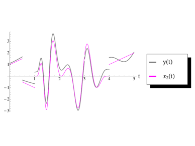
Figure 1: Observation’s noise

The sub-optimal estimation $\hat{x}(t,\varepsilon)$ and error are given by

$$\begin{split}&\hat{x}_{t}(t,\varepsilon)=\bigr{[}-1-K(1+\frac{2c_{3}^{2}(t)}{\varepsilon\exp(\sqrt{t})})\bigl{]}\hat{x}(t,\varepsilon)+\frac{6y(t)}{6+T\varepsilon},\hat{x}(\varepsilon,0)=0,\\ &K_{t}=-2K-(1+\frac{2c_{3}^{2}(t)}{\varepsilon\exp(\sqrt{t})})K^{2}+\varepsilon(1+\frac{1}{\frac{6}{T}+\varepsilon}),\,K(0,\varepsilon)=0,\\ &\hat{\sigma}(t,\varepsilon):=\frac{1}{\varepsilon}\bigr{[}\frac{K(t,\varepsilon)}{(K(t,\varepsilon)+1)^{2}}-\int_{0}^{t}[K^{2}(s,\varepsilon)+\frac{\varepsilon^{2}}{(\frac{6}{T}+\varepsilon)^{2}}]z^{\varepsilon}(s;t)^{2}ds\bigl{]},\\ &z_{t}^{\varepsilon}(t;\tau)=[1+K(1+\frac{2c_{3}^{2}(t)}{\varepsilon\exp(\sqrt{t})})]z^{\varepsilon}(t;\tau),z^{\varepsilon}(\tau,\tau)=(K(\tau,\varepsilon)+1)^{-1}\end{split}$$

Note that the pencil $sF^{\prime}-C^{\prime}-H^{\prime}H$ is regular. As (31) is solvable in this case we apply Proposition 7 in order to derive the minimax estimation $\hat{x}$ and minimax estimation error $\hat{\sigma}(t)$:

$$\begin{split}&\hat{x}_{t}=\bigr{[}-1-K(t)\frac{2c_{3}^{2}(t)}{\exp(\sqrt{t})})\bigl{]}\hat{x}+y(t),\quad\hat{x}(0)=0,\\ &K_{t}=-2K-\frac{2c_{3}^{2}(t)}{\exp(\sqrt{t})})K^{2}+(1+\frac{T}{6}),\,K(0,\varepsilon)=0,\\ &\hat{\sigma}^{2}(t,\ell_{1}):=K(t)\ell_{1}^{2}\end{split}$$

In Figure 2 the comparison of the optimal estimator $\hat{x}$ and error $\hat{\sigma}(t)$ with sub-optimal estimator $\hat{x}(\varepsilon)$ and error $\hat{\sigma}(t,\varepsilon)$ are presented, provided $\varepsilon=\exp(-100)$ and $\ell_{1}=0$.

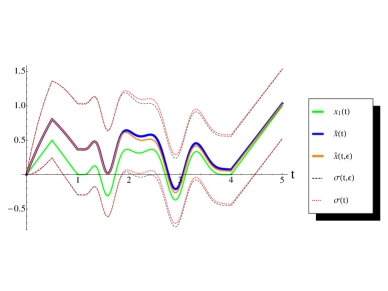
Figure 2: Optimal estimation and error, suboptimal estimation and error and $x_{1}$

References

- Albert (1972) Albert, A. (1972). Regression and the Moor-Penrose pseudoinverse. Acad. press, N.Y.
- Becerra et al. (2001) Becerra, V., Roberts, G., and Griffiths, G. (2001). Applying the extended kalman filter to systems described by nonlinear differential-algebraic equations. Control Engineering Practice, 9, 267–281.
- Bertsekas and Rhodes (1971) Bertsekas, D. and Rhodes, I.B. (1971). Recursive state estimation with a set-membership description of the uncertainty. IEEE Trans. Automat. Contr., AC-16, 117–128.
- Brammer and Siffling (1989) Brammer, K. and Siffling, G. (1989). Kalman Bucy Filters. Artech House Inc., Norwood MA, USA.
- Campbell (1987) Campbell, S. (1987). A general form for solvable linear time varying singular systems of differential equations. SIAM J. Math. Anal., 18(4).
- Campbell et al. (1991) Campbell, S., Nichols, N., and Terrell, W. (1991). Duality, observability, and controllability for linear time-varying descriptor systems. Circuits Systems Signal Process, 10(4).
- Campbell and Petzold (1983) Campbell, S. and Petzold, L. (1983). Canonical forms and solvable singular systems of differential equations. SIAM J.Alg.Discrete Methods, 4, 517–521.
- Darouach et al. (1997) Darouach, M., Boutayeb, M., and Zasadzinski, M. (1997). Kalman filtering for continuous descriptor systems. In ACC, 2108–2112. AACC, Albuquerque.
- Eremenko (1980) Eremenko, V. (1980). Reduction of the degenerate linear differential equations. Ukr. Math. J., 32(2), 168–172.
- Frankowska (1990) Frankowska, H. (1990). On controllability and observability of implicit systems. System & Control Letters, 14, 219–225.
- Gantmacher (1960) Gantmacher, F. (1960). The theory of matrices. Chelsea Publish.Comp., N.-Y.
- Gerdin et al. (2007) Gerdin, M., Schön, T.B., Glad, T., Gustafsson, F., and Ljung, L. (2007). On parameter and state estimation for linear differential-algebraic equations. Automatica, 43(3), 416–425.
- Ilchmann and Mehrman (2005) Ilchmann, A. and Mehrman, V. (2005). A behavioral approach to time-varying linear systems. part 2: Descriptor systems. SIAM J. Control Optim., 44, 1748–1765.
- Kurina and März (2007) Kurina, G. and März, R. (2007). Feedback solutions of optimal control problems with DAE constraints. SIAM J. Control Optim., 46(4), 1277–1298.
- Kurzhanski and Valyi (1997) Kurzhanski, A. and Valyi, I. (1997). Ellipsoidal Calculus for Estimation and Control. Birkhäuser, Boston.
- Luenberger and A. (1977) Luenberger, D. and A., A. (1977). Singular dynamic leontief systems. Econometrica, 45(4), 234–243.
- Mehrmann and Stykel (2005) Mehrmann, V. and Stykel, T. (2005). Descriptor systems: a general mathematical framework for modelling, simulation and control. Technical Report 292-2005, DFG Research center Matheon, Berlin. Www.matheon.de.
- Milanese and Tempo (1985) Milanese, M. and Tempo, R. (1985). Optimal algorithms theory for robust estimation and prediction. IEEE Trans. Autom. Contr., 30(8), 730–738.
- Mills (2006) Mills, J. (2006). Dynamic modelling of a a flexible-link planar parallel platform using a substructuring approach. Mechanism and Machine Theory, 41, 671–687.
- Muller (1998) Muller, P. (1998). Stability and optimal control for nonlinear descriptor systems: A survey. Appl. Math. Comput. Sci., 8(2), 269–286.
- Nakonechny (1978) Nakonechny, A. (1978). Minimax estimation of functionals defined on solution sets of operator equations. Arch.Math. 1, Scripta Fac. Sci. Nat. Ujer Brunensis, 14, 55–60.
- Ozcaldiran and Lewis (1989) Ozcaldiran, K. and Lewis, F. (1989). Generalized reachability subspaces for singular systems. SIAM J. Control and Optimization, 27, 495–510.
- Rabier and Rheinboldt (1994) Rabier, P. and Rheinboldt, W. (1994). A geometric treatment of implicit differential-algebraic equations. J.Differential Equtions, 109, 110–146.
- Rabier and Rheinboldt (1996) Rabier, P. and Rheinboldt, W. (1996). Time-dependent linear dae with discontinuous input. Lin. Algeb. & Appl., 247, 1–29.
- Reich (1990) Reich, S. (1990). On a geometrical interpretation of differential-algebraic equations. Circuits Systems Signal Process, 9(4).
- Reis (2008) Reis, T. (2008). Circuit synthesis of passive descriptor systems—a modified nodal approach. Int. J. Circ. Theor. Appl.
- Rutkas (1975) Rutkas, A. (1975). Cauchy’s problem for the equation . Diff.Equations (translation of Diff. uravn.), 11, 1486–1497.
- Samoilenko et al. (2000) Samoilenko, A., Shkil, M., and Yakovets, V. (2000). Degenerate systems of linear differential equations. Kyiv, Vysha shkola.
- Shlapak (1975) Shlapak, U. (1975). Periodical solutions of degenerate linear differential equations. Ukr. Math. J., 27(2), 137–140.
- Tikhonov and Arsenin (1977) Tikhonov, A. and Arsenin, V. (1977). Solutions of ill posed problems. Wiley, New York.
- Xu and Lam (2006) Xu, S. and Lam, J. (2006). Robust control and filtering of singular systems. Lect.notes in Control and Information Scienses, 332, 1–231.
- Zhuk (2007) Zhuk, S. (2007). Closedness and normal solvability of an operator generated by a degenerate linear differential equation with variable coefficients. Nonlin. Oscillations, 10, 1–18.
- Zhuk (2009a) Zhuk, S. (2009a). Set-membership state estimation for uncertain non-causal discrete-time linear DAEs. URL http://arxiv.org/abs/0807.2769. Preprint, under revision in the Automatica journal, http://arxiv.org/abs/0807.2769.
- Zhuk (2009b) Zhuk, S. (2009b). State estimation for a dynamical system described by a linear equation with unknown parameters. Ukrainian Mathematical Journal, 61(2), 178–194. Http://arxiv.org/abs/0810.3295.