A sub-resolution multiphase interstellar medium model of star formation and SNe energy feedback

Abstract

We present a new multi-phase sub-resolution model for star formation and feedback in SPH numerical simulations of galaxy formation. Our model, called MUPPI (MUlti-Phase Particle Integrator), describes each gas particle as a multi-phase system, with cold and hot gas phases, coexisting in pressure equilibrium, and a stellar component. Cooling of the hot tenuous gas phase feeds the cold gas phase. We compute the cold gas molecular fraction using the phenomenological relation of Blitz & Rosolowsky between this fraction and the external disk pressure, that we identify with the SPH pressure. Stars are formed out of molecular gas with a given efficiency, which scales with the dynamical time of the cold phase. Our prescription for star formation is not based on imposing the Schmidt-Kennicutt relation, which is instead naturally produced by MUPPI. Energy from supernova explosions is deposited partly into the hot phase of the gas particles, and partly to that of neighboring particles. Mass and energy flows among the different phases of each particle are described by a set of ordinary differential equations which we explicitly integrate for each gas particle, instead of relying on equilibrium solutions. This system of equations also includes the response of the multi-phase structure to energy changes associated to the thermodynamics of the gas. Our model has an intrinsically runaway behavior: energy from supernovae increases gas pressure which increases in turn the star formation rate through the molecular fraction. This runaway is stabilized in simulations by the hydrodynamic response of the gas: when it receives enough energy, it expands thereby decreasing its pressure.

We apply our model to two isolated disk galaxy simulations and two spherical cooling flows. MUPPI is able to reproduce the Schmidt-Kennicutt relation for disc galaxies. It also reproduces the basic properties of the inter-stellar medium in disc galaxies, the surface densities of cold and molecular gas, of stars and of star formation rate, the vertical velocity dispersion of cold clouds and the flows connected to the galactic fountains. Quite remarkably, MUPPI also provides efficient stellar feedback without the need to include a scheme of kinetic energy feedback.

1 Introduction

Numerical simulations are a powerful tool to study structure formation and evolution in a cosmological context, and their use has become standard in the last decades. The gravitational evolution of the concordance $\Lambda$ Cold Dark Matter ($\Lambda$CDM) model is now studied and understood in detail through N-body simulations covering large dynamic ranges. However, a direct comparison of the results of numerical simulations with observations clearly requires the treatment of baryonic physics. Moreover, while $\Lambda$CDM cosmogony is quite successful in reproducing the observed large-scale properties of the Universe (Springel et al., 2006), on galactic scales a number of issues, like ab-initio formation of disk galaxies and abundance and properties of small “satellite” galaxies (see, e.g., Mayer et al., 2008, for a review) , are still debated.

Including astrophysical processes in simulations such as radiative gas cooling, star formation and energy feedback from Supernovae (SNe) (see e.g. Dolag et al., 2008, for a review), is a hard task for several reasons. The physics of star formation is complex and currently not understood in detail; moreover, the dynamical range needed to simultaneously resolve the formation of cosmic structures and the formation of stars is huge, since the former process happens on Mpc scales and the latter on sub-pc scales.

Several authors included simple schemes to transform the cold dense gas (depicted as a single fluid) into stars (e.g. White & Rees, 1978, Cen & Ostriker, 1992, Navarro & White, 1993, Katz et al., 1996). For instance, Katz et al., 1996 based their recipe of star formation simply on an overdensity criterion, thus ignoring the multi-phase nature of the Inter-Stellar Medium (ISM). However, in the ISM of observed galaxies, the gas is not single-phase, being instead characterized by a wide range of density and temperature states, as illustrated, e.g., by Cox (2005). As shown in this review, such a multi-phase medium results from the interplay of processes such as gravity, hydrodynamics, turbulence, heating by SNe and stellar winds, magnetic fields, cosmic rays, chemical enrichment and dust formation. The problem of star formation can thus be dealt with algorithms which explicitly model, to some level of approximation, the multi-phase structure of the ISM. A number of recipes to tackle such a problem has been proposed (Yepes et al., 1997, Thacker & Couchman, 2000, Springel & Hernquist, 2003, Marri & White, 2003, Scannapieco et al., 2006, Stinson et al., 2006, Booth et al., 2007, Dalla Vecchia & Schaye, 2008). While not all of them make an attempt to model the multi-phase behavior of single gas particles, the aim of all these prescriptions is to reproduce some basic observations like the Schmidt-Kennicutt (SK) relation (Kennicutt, 1998b) while regulating the final amount of stars with energetic feedback from Type II and, sometimes, Type Ia SNe. Still, only a few of these prescriptions include some realistic (though necessarily simplified) modeling of a multi-phase, turbulent ISM.

Early attempts to introduce stellar feedback into simulations (Baron & White, 1987, Cen & Ostriker, 1992, Katz, 1992, Navarro & White, 1993) already showed that if SN energy is deposited as thermal energy onto the star-forming gas particle, it is quickly dissipated through radiative cooling before it has any relevant effects. This is due to the fact that the characteristic timescale of radiative cooling at the typical density of star-forming regions is far shorter then the free-fall gravitational timescale (Katz, 1992).

Several solutions have been proposed to increase the efficiency of feedback in regulating star formation. For instance, Springel & Hernquist (2003) introduced a sub-resolution description of a two-phase ISM. In their model, the amount of gas in the cold and hot phases is regulated by the thermodynamical properties of the star-forming gas particle: the two phases are always considered to be in thermal pressure equilibrium. Star formation is proportional to the amount of gas in the cold phase. Thermal energy of Type II SN participates in the determination of equilibrium between the phases; since the particle interacts hydrodynamically using its average temperature, the efficiency of such a feedback is not high enough to suppress star formation to observed level. For this reason, Springel & Hernquist (2003) also included a phenomenological prescription of kinetic feedback, in which star-forming gas particles are stochastically selected to receive a velocity “kick”, with probability proportional to their star formation rate (SFR hereafter), and hydrodynamically decouple for a given time from the surrounding gas.

Scannapieco et al. (2006) tried to overcome the overestimation of the cooling rate by decoupling gas phases using separate thermodynamic variables i.e. hot, diffuse gas particles do not “see” cold, dense gas particles as neighbors. Booth et al. (2007) took a different approach and decoupled the cold molecular phase from the hot phase by describing the former with sticky particles and treating their aggregations with a sub-resolution kinetic coagulation model. Dalla Vecchia & Schaye (2008) implemented a variation of Springel & Hernquist (2003) prescription in which winds are produced locally by neighboring star-forming particles and are not hydrodynamically decoupled. These authors showed that coupled winds generate a large bipolar outflow in a dwarf-like galaxy and a galactic fountain in a massive galaxy, while the Springel & Hernquist (2003) decoupled wind produces isotropic outflows in both cases.

A different solution consists in simply suppressing radiative cooling of gas particles which have just been heated by SNe (typically for 30 Myr, the observed lifespan of a SN blast: Gerritsen & Icke, 1997, Thacker & Couchman, 2000, Sommer-Larsen et al., 2003). Apart from providing an artificial method for reducing cooling and star formation rates, this scheme is strongly resolution-dependent (e.g., Thacker & Couchman, 2000). Stinson et al. (2006) found a numerical implementation able to partly remove the dependence on resolution. This was used by Governato et al. (2007) in a cosmological simulation of a disk galaxy, and was demonstrated to be very efficient in reducing the angular momentum loss of gas by pushing it in the outskirts of DM haloes while they merge.

Very recently, direct simulations of the ISM in extended galaxies have become computationally feasible. For instance, Pelupessy et al. (2006); Robertson & Kravtsov (2008); Tasker & Bryan (2008) simulated isolated galaxies with a force resolution of tens of pc, explicitly following the formation of molecular clouds, while Ceverino & Klypin (2009) simulated the formation and evolution of a disk galaxy in a cosmological context (but only up to redshift $z\sim 3$) with comparable resolution. Such first works show that it is possible to simulate galaxies with reasonable ISM properties; however, applying these codes to a cosmological box having sizes of $\ga 10$ Mpc will be unfeasible for several years to come. This confirms the necessity of developing realistic sub-resolution models of star formation and feedback, which are able to capture in a physically motivated way the complex nature of star formation and energy feedback.

In this paper, we present a novel algorithm of this kind, MUPPI (MUlti-Phase Particle Integrator), implemented in the GADGET-2 Tree-SPH code (Springel, 2005). It is based on a modified version of the analytic model of star formation and feedback in a two-phase ISM developed by Monaco (2004b) (M04 hereafter). The main characteristic of this algorithm is that it performs, for each multi-phase (MP) gas particle, the integration of a system of ordinary differential equations that regulate mass and energy flows among the ISM phases. This integration is performed within the SPH time-step, and allows to follow all the transients of the system, instead of assuming an equilibrium solution for the ISM, which in fact turns out to never be in equilibrium. The model is heavily based on the assumption of a correlation between the ratio of molecular to neutral hydrogen and gas pressure. Such relation has been observed to hold in local galaxies by Blitz & Rosolowsky (2004, 2006), and is used as a phenomenological prescription to bypass the need of a detailed description of molecular cloud formation. The interaction between MUPPI and the SPH part of GADGET-2 allows each particle to immediately respond to the injected energy; because most thermal energy is contained in the diluted hot phase, the cooling time of MP particles is relatively long, thus allowing an efficient injection of thermal energy.

The organization of the paper is as follows. Section 2 provides a detailed description of MUPPI: the scientific rationale behind it, the system of equations, the entrance and exit conditions, the stochastic star formation algorithm, the interaction with SPH, the redistribution of energy to neighboring particles. Section 3 presents the suite of numerical tests performed to assess the validity of the code. We describe here the results of simulations carried out for (i) an isolated Milky Way-like (MW) galaxy, (ii) an isolated Dwarf-like (DW) galaxy, (iii) two analogous isolated, non-rotating haloes with gas initially in hydrostatic equilibrium. We finally report on a study of resolution dependence and exploration of model parameter space. We summarize our main results and conclusions in Section 4.

2 The model

A successful sub-resolution model for hydrodynamical simulations of galaxy formation should find the best compromise between simplicity of implementation and complexity of evolution, aiming at describing as closely as possible the behavior of star-forming regions.

Our starting point is the M04 analytic model of star formation and feedback. In that paper the ISM is described as a two-phase medium in thermal pressure equilibrium. The formation of molecular clouds is due to the balance between kinetic aggregations and gravitational collapse of super-Jeans clouds. SNe exploding in molecular clouds give raise to super-bubbles that sweep the ISM. The energy given to the ISM by the blast is explicitely computed under the simple assumption that this propagates into the most pervasive and diluted hot phase (Ostriker & McKee, 1988). Different regimes of feedback are found, according to whether the super-bubbles are able (or not) to blow out of the system before they are pressure-confined by the hot phase.

The M04 model was constructed to shed light on the way energy from SNe is given to the ISM, and to quantify the efficiency of this process as a function of fundamental environmental parameters like gas surface density or galaxy vertical scale-length. However, we consider the M04 model unsuitable for a direct implementation in an SPH code, for several reasons. First, the system on which the M04 model is constructed consists of a region of ISM which contains many cold and star-forming clouds. The mass of a molecular cloud can reach $\sim 10^{7}$ M_⊙ in the Milky Way, while particle masses in simulations of isolated galaxies can range from $10^{4}$ to $10^{6}$ M_⊙. Clearly, a single star-forming cloud will be sampled by many particles in realistic cases, so that the starting assumption of M04 should be revised.

Our approach here is to consider each SPH gas particle as a potential parcel of the multi-phase ISM, when its density and temperature allows it. Whenever this is the case, the gas particle will samples the ISM for a period of time, during which it represents both part of a giant molecular cloud and part of the tenuous hot gas. The sampled molecular cloud is assumed to be destroyed after some time, after which the gas particle becomes again single phase. It can become again multi-phase, in case it is allowed by its physical conditions, thus sampling another portion of the ISM. Gas particles are therefore allowed to have several distinct multi-phase stages.

Second, in M04 the system is open, receiving mass from and ejecting mass (and energy) to an external reservoir, called “Halo”. In a typical simulation infall and outflow of gas in/from the galaxy will be resolved. For simplicity of implementation, we prefer to neglect any inward or outward mass flow in our subgrid model, only taking into account external energy flows.

Third, M04 explicitly computes the energy received by the hot phase of the ISM from expanding super-bubbles generated by multiple SNe explosions in star-forming clouds. Our choice here is to parameterize such process by assuming that the hot phase receives a constant fraction of the produced SN energy, using M04 and Monaco (2004a) to suggest fiducial values for the parameters. This approach has the advantage of giving a much simpler and transparent grasp to the distribution of energy.

Fourth, an important feature of the M04 model is to predict different behavior for systems with different geometries: depending on the cold gas surface density, in a “thin” disk system super-bubbles will manage to blow out, thus dispersing most energy in the vertical direction, while in a “thick” system most energy will be deposited into the local ISM, thus leading to much higher pressure. In a hydro simulation the geometry of the system is resolved, at least within the force resolution of the code. The question is then whether the vertical scale-length of the system may be guessed starting from a particle’s local (in the SPH sense) neighborhood, and the two different regimes inserted in the sub-resolution model. We choose to avoid this guess and adopt a different strategy: all particles behave like in the “thin system” case of M04, i.e. they inject energy to neighboring particles along the “least resistance path” defined by (minus) the gradient of the SPH density. In a truly thin disk this energy will be directed outwards, while in a thick or very dense system the energy will be trapped within the star-forming region. In other words, the “thin” or “thick” regimes are resolved by the simulation instead of being assumed as part of the sub-resolution model.

A further fundamental difference is related to the modeling of star-forming (molecular) cloud masses, which is done in M04 using a kinetic aggregation model. However, different authors (Blitz & Rosolowsky, 2004, 2006; Leroy et al., 2009) have shown that in local galaxies the ratio between the surface densities of molecular and cold gas scales almost linearly with the so-called “external pressure”, defined as the total pressure required at the midplane to support a hydrostatic disc. This behavior is not obtained in the M04 kinetic approach, where pressure determines the size of clouds and higher pressure implies smaller clouds and then smaller cross section. As a result, a higher pressure results in a smaller fraction of cold mass in molecular clouds, which is clearly at variance with observations. These observations are naturally explained in a context in which pressure is driven by turbulence and molecular cooling in the turbulent ISM is properly taken into account (Robertson & Kravtsov, 2008). M04 assumed that the formation of “molecular” (star-forming) clouds is triggered by gravitational collapse through a Jeans-like criterion, and this may well be a naive description of the dynamics of the ISM. We then adopt the strategy of using the observed relation of Blitz & Rosolowsky (2006) to construct a phenomenological model that computes the fraction of molecular gas, thus bypassing all the difficulties connected with the poorly understood formation of molecular clouds. We use the SPH pressure of the particle in place of the external pressure. Clearly the use of a relation found for local galaxies and not tested at high redshift should be considered as an anstatz to the true solution. However, star formation in high redshift galaxies is known to take place in more gas-rich, compact, pressurized and molecular-dominated environments than in local galaxies. Therefore, an evolution of this relation with redshift should have a minor impact.

We have implemented our model in a version of the GADGET-2 code which adopts an explicitly entropy-conserving SPH formulation, and includes radiative cooling computed for a primordial plasma with vanishing metalicity (Springel & Hernquist, 2003).

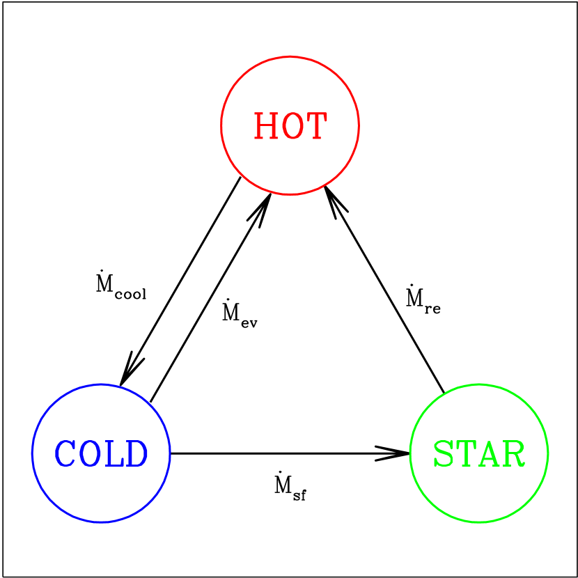
Figure 1: Schematic illustration of the mass flows between the different phases.

2.1 The sub-resolution model

We assume that a MP SPH particle is made up of two gas phases, namely cold and hot gas, and a stellar component. The two gas phases are assumed to be in thermal pressure equilibrium:

$$n_{\rm h}\cdot T_{\rm h}=n_{\rm c}\cdot T_{\rm c}$$ (1)

Here and in the following $n$ denotes particle number density, e.g. $n_{\rm h}=M_{\rm h}/(\mu_{\rm h}m_{p})$, where $m_{p}$ is the proton mass, $\mu_{\rm h}=4/(5f_{\rm HI}+3)\simeq 0.6$ and $\mu_{\rm c}=4/(3f_{\rm HI}+1)\simeq 1.2$ are the molecular weights, $f_{\rm HI}=0.76$ being the fraction of neutral hydrogen. To most effectively single out the behavior of MUPPI, we decided to develop and test the code neglecting any chemical evolution. This means that the molecular weights of the hot and cold phases are constant and the cooling time is computed for a gas with zero metalicity.

The temperature of the cold phase is set to $T_{\rm c}=1000$ K; this is in line with Springel & Hernquist (2003). This temperature regulates the duration of each multi-phase stage and the star formation rate: the lower $T_{\rm c}$ is, the shorter the multi-phase stage and the higher the star formation rate. The value we chose gives multi-phase stages lasting some tens of million years and a reasonable SFR (see below, Section 3.6). If $F_{\rm h}$ is the fraction of gas mass in the hot phase, then its filling factor $f_{\rm h}$ is:

$$f_{\rm h}=\frac{1}{1+\frac{F_{\rm c}}{F_{\rm h}}\cdot\frac{\mu_{\rm h}}{\mu_{\rm c}}\cdot\frac{T_{\rm c}}{T_{\rm h}}}$$ (2)

with $f_{\rm c}=1-f_{\rm h}$. Mass is exchanged among the components as in Figure 1. A fraction $f_{\rm mol}$ of the cold gas will be in molecular form, and another fraction $f_{\star}$, per dynamical time $t_{\rm dyn}$ of the molecular cold phase, will be consumed into stars. The dynamical time is:

$$t_{\rm dyn}=\sqrt{\frac{3\pi}{32G\rho_{\rm c}}}\simeq 5.15\cdot 10^{7}(\mu_{\rm c}n_{\rm c})^{-1/2}\ {\rm yr}$$ (3)

This gives rise to a star formation rate of:

$$\dot{M}_{\rm sf}=f_{\star}\cdot\frac{f_{\rm mol}\cdot M_{\rm c}}{t_{\rm dyn}}$$ (4)

As mentioned above, we compute the fraction of molecular gas, $f_{\rm mol}$, using the results of Blitz & Rosolowsky (2006), that can be recast as follows:

$$f_{\rm mol}=\frac{1}{1+P_{0}/P}$$ (5)

where P is the pressure. Note that here for simplicity we adopt a linear scaling with pressure, in place of the $0.92\pm 0.07$ exponent found in Blitz & Rosolowsky (2006). Following this paper, the pressure $P_{0}$ at which half of the cold gas is molecular is set to $P_{0}/k_{B}=35000$ K cm^-3, with $k_{B}$ being the Boltzmann constant. As mentioned above, we use the SPH pressure as an estimate of the external one.

A fraction $f_{\rm re}$ of the mass involved in star formation is promptly restored to the hot phase through the death of massive stars:

$$\dot{M}_{\rm re}=f_{\rm re}\cdot\dot{M}_{\rm sf}$$ (6)

We use $f_{\rm re}=0.2$, roughly consistent with a Salpeter stellar Initial Mass Function (IMF). Since we neglect metal production, the restored material will have the same composition as the original one. Radiative cooling creates a cooling flow which is modeled as follows:

$$\dot{M}_{\rm cool}=\frac{M_{\rm h}}{t_{\rm cool}}$$ (7)

where $t_{\rm cool}$ is the radiative cooling time derived from the GADGET-2 cooling function which uses the tabulated cooling rates given by Katz et al. (1996). Following M04 and Monaco (2004a), the evaporation rate is not connected to thermal conduction within the expanding super-bubbles, as in McKee & Ostriker (1977) and in Springel & Hernquist (2003), but with the destruction of the molecular cloud by the action of massive stars. Monaco (2004a) estimates that $\sim 10$ per cent of the cloud is evaporated, the rest being snow-ploughed back to the cold phase by the first SNe that explode in the cloud. We then model the evaporation flow as:

$$\dot{M}_{\rm ev}=f_{\rm ev}\cdot\dot{M}_{\rm sf}$$ (8)

where $f_{\rm ev}=0.1$ in our runs, as suggested by Monaco (2004a).

Calling $M_{\star}$, $M_{\rm c}$ and $M_{\rm h}$ the mass in stars and in the cold and hot gas phases, the resulting system for the mass flows is:

$$\dot{M}_{\star}=\dot{M}_{\rm sf}-\dot{M}_{\rm re}$$ (9)

$$\dot{M}_{\rm c}=\dot{M}_{\rm cool}-\dot{M}_{\rm sf}-\dot{M}_{\rm ev}$$ (10)

$$\dot{M}_{\rm h}=-\dot{M}_{\rm cool}+\dot{M}_{\rm re}+\dot{M}_{\rm ev}$$ (11)

Energy flows are associated to mass flows. We follow the evolution of the thermal energy of the hot phase, $E_{\rm h}$, that is connected to its temperature as follows:

$$T_{\rm h}=\frac{E_{\rm h}}{M_{\rm h}}\frac{(\gamma-1)\mu_{\rm h}m_{p}}{k_{B}}$$ (12)

where we assume $\gamma=5/3$ for the adiabatic index of a mono-atomic gas. Energy is lost by cooling and acquired from SN explosions. Moreover, energy is exchanged with other particles through the hydro energy term $\dot{E}_{\rm hydro}$, provided by the SPH part of the code, which gives the energy variation due to adiabatic contraction/expansion, shocks etc. The cooling term is simply:

$$\dot{E}_{\rm cool}=\frac{E_{\rm h}}{t_{\rm cool}}$$ (13)

while we assume that a small fraction $f_{\rm fb,local}=0.02$ of the SN energy is directly injected into the local ISM:

$$\dot{E}_{\rm heat,local}=E_{\rm SN}\cdot f_{\rm fb,local}\cdot\frac{\dot{M}_{\rm sf}}{M_{\rm\star,SN}}\,.$$ (14)

Here $E_{\rm SN}$ is the energy of one single SN and $M_{\star\rm,SN}$ the mass of stars formed for each SN. We assume for this parameter a value of 120 M_⊙, roughly compatible with a Salpeter IMF, once we assume a limiting mass of 8 M_⊙ for the stars exploding as type-II SNe. The exact value of $f_{\rm fb,local}$ has a small influence on the behavior of our model, as long as the energy injected in the local ISM is not larger than that distributed to neighbors. We note that in our model, when a particle is multi-phase, radiative cooling only involves its hot phase.

The resulting equation for the evolution of the hot phase thermal energy is:

$$\dot{E}_{\rm h}=\dot{E}_{\rm heat,local}-\dot{E}_{\rm cool}+\dot{E}_{\rm hydro}\qquad\qquad$$ (15)

The term $\dot{E}_{\rm hydro}$ also includes the energy contributed by SN explosions within neighboring MP particles. This energy is computed distributing a fraction $f_{\rm fb,out}$ of SN energy to neighboring particles. This point will be further discussed in Section 2.4.

In this version of the code we do not attempt to model the evolution of the kinetic energy of the cold phase, which would give a kinetic pressure term. We tested some simple implementations and noticed that they added to the complexity (and number of parameters) of the formulation without giving any obvious improvement, so we prefer here to keep the simpler formulation.

2.2 Entrance and exit conditions from multi-phase and the SPH/MUPPI interface

A particle enters the multi-phase regime whenever its density is higher than the threshold value $n_{\rm thr}=0.01$ cm^-3 and its temperature is below $T_{\rm thr}=5\times 10^{4}$ K. Since pressure determines the molecular fraction (equation 5), and thus the cut in the SK relation, we use a very low value of the density threshold such that most particles in our tests are always in multi-phase regime. Moreover, a temperature threshold is imposed to prevent hot dense gas particles to spuriously become multi-phase. As soon as a particle becomes multi-phase, it is then initialized with all of its mass in the hot phase, although the temperature is relatively low at the beginning.

At this point, all the gas mass is in the hot phase, and maintains its SPH density. Its temperature is obtained from the SPH entropy. During the first stage of the multi-phase evolution, the hot gas cools and deposits mass onto the cold phase. If pressure is sufficiently high, a fraction of such a cold gas is treated as molecular and gives rise to star formation. Then, SN feedback heats the remaining hot gas and also evaporates some of the cold gas, moving it to the hot phase, thus contrasting the cooling flow.

The two gas phases and the stellar component are clearly constrained to stay within the same volume. However, in a realistic case these two phases should not respond in the same way to pressure forces, because the hot phase tends to flow away while the cold phase is only partially dragged. In other words, describing a star-forming, multi-phase ISM as a single particle cannot be valid over a long time. For this reason, we decide to use a single time-scale to regulate both star formation rate of a multiphase particle and the duration of the multi-phase stage.

We use the dynamical time of the cold phase (equation 3), but we keep it fixed when, for the first time since the start of the multi-phase stage, the mass fraction in the cold phase exceeds 95 per cent of the total mass. Cooling of the hot phase is very fast for many MP particles and the condition of 95 per cent of cooled mass is usually met within the first MUPPI integration. On the other hand, particles that enter in the multi-phase stage with temperature $T\la 10^{4}$ K, i.e. when all hydrogen is neutral and no effective coolant is present, have to wait until the temperature rises (by compression of by feedback from other star-forming particles) to start depositing mass into the cold phase.

This dynamical time $t_{\rm dyn}$ thus regulates both star formation and the exit from the multi-phase stage. We adopt M04 suggestion fixing $t_{\rm clock}=2t_{\rm dyn}$; this is the typical time after which the molecular cloud that gives rise to star formation is destroyed. In this way, the particle exits from the multi-phase stage after the time $t_{\rm clock}$ has elapsed since the ”freezing” of the dynamical time discussed above. Moreover, the particle also exits the multi-phase stage whenever its SPH density drops below $n_{\rm out}=(2/3)n_{\rm thr}$. Usually, a multi-phase stage lasts for tens or up to hundreds of simulation time-steps. We evaluate our exit conditions before the multi-phase integration takes place. Therefore, when a particle exits its multi-phase stage, it maintain its SPH entropy as given by the SPH calculation.

Within each SPH time-step, MUPPI is implemented in the GADGET-2 flow as follows: (i) SPH densities $\rho$ of gas particles are evaluated in the standard way, along with gravitational and hydrodynamical forces; (ii) MUPPI integration is performed for single-phase particles that match the entrance criterion and for multi-phase particles that did not match the exit criterion at the previous time-step; (iii) stochastic star formation on multi-phase particles is performed; (iv) SN energy is distributed to neighboring particles.

More in detail, MUPPI integration in the above step (ii) proceeds as follows. For each particle, the increase in entropy $dS$ resulting from the computation of hydrodynamic forces, is translated into an energy increment $dE_{\rm hydro}=E_{\rm new}-E_{\rm ave,old}$. Note that such an energy increment includes the effect of an adiabatic expansion or compression, if the density of the particle has changed since the previous time-step. We use the new SPH density to convert entropy to energy at the beginning of our MUPPI integration, so the difference with the previous value of the particle average energy $E_{\rm ave,old}$ includes the $PdV$ work. The energy $E_{\rm new}$ also includes contribution due to SNe feedback coming from neighboring particles (see Section 2.4).

Then, the energy flux $\dot{E}_{\rm hydro}$ is calculated, by dividing the energy increment by the duration of the SPH time-step. This energy is gradually injected into (or extracted from) the hot phase during the integration (equation 15). Since $\dot{E}_{\rm hydro}$ includes the effect of the entropy change $\Delta S$ due to hydrodynamics, $\Delta S$ itself is set to zero.

The evolution of properties of the ISM represented by the MP gas particle is then calculated by integrating equations 9, 10, 11 and 15 for the duration of the SPH time-step. The average density of a MP particle never changes during a multi-phase integration, while the cold and hot number densities, $n_{c}$ and $n_{h}$, evolve according to our system of ordinary differential equations.

At the end of the integration, the updated entropy of the particle is re-assigned based on the final mass-averaged thermal energy, $E_{\rm ave,new}$, and on the density, $\rho$, of the same particle:

$$S_{\rm new}=(\gamma-1)\frac{E_{\rm ave,new}}{\rho_{\rm ave,new}^{\gamma-1}}\,.$$ (16)

As a consequence of the pressure equilibrium hypothesis, the mass-averaged values used to compute the final energy and entropy provide a particle pressure which is equal to that of the hot and cold MUPPI phases. This allows the particle to respond hydrodynamically to the energy injection and pressurization caused by stellar feedback. At the same time, cooling of the MP particles is performed by MUPPI on the basis of the hot phase density. In this way the injected energy is not quickly radiated away since the hot phase density is much lower than the average density. The energy $E_{\rm ave,new}$ will be used at the beginning of the next multi-phase integration to estimate the term $dE_{\rm hydro}$.

At relatively low pressure, when the molecular fraction and thus the star formation rate is low, it can happen that the cooling caused by an expansion (and driven by $\dot{E}_{\rm hydro}$ in the energy equation) leads to a catastrophic loss of hot phase thermal energy. In this case the energy input from SNe is too low to substain a multi-phase ISM, so we simply force the particle to exit the multi-phase regime.

Finally, it can happen that a gas particle is supposed to spawn a star (see Section 2.3 for details), but its mass in stars and cold gas is less than the mass of the star to be spawned. In this rather unlikely event we force the gas particle to exit the multi-phase stage. It is the only case in which the exit happens after an multi-phase integration; the SPH entropy is set to $S_{\rm new}$.

2.3 Stochastic star formation

Star formation is implemented with the stochastic algorithm of Springel & Hernquist (2003). In an SPH time-step, MUPPI transforms a mass $\Delta M_{\star}$ of gas into stars. If $M_{p}=M_{\rm h}+M_{\rm c}+M_{\star}$ is the total particle mass, then a star particle of mass $M_{p\star}$ is spawned by the gas particle with probability:

$$P=\frac{M_{p}}{M_{p\star}}\left[1-\exp\left(-\frac{\Delta M_{\star}}{M_{p}}\right)\right]$$ (17)

The mass of the spawned star is set as a fraction $1/N$ of the initial mass of gas particles, so as to have $N$ generations of stars per gas particle. In the following we use $N=4$ as a reasonable compromise between the needs of providing a continuous description of star formation and of preventing profileration of low-mass star particles. The mass of the spawned star particle is taken from the mass $M_{\star}$ of the stellar component of the MP particle and, if this is insufficient, from the cold phase. If the spawning consumes also all of the cold phase, then the particle exits the multi-phase regime.

Whenever a particle exits the multi-phase regime, its accumulated stellar component, that has not been used to spawn a star, is nulled. This is consistent with stochastic star formation: the sub-resolution model determines the probability of spawning a star, but this probability is connected with the amount of stars formed in an SPH time-step and not with the stellar mass accumulated in a MP gas particle.

2.4 Redistribution of energy to neighboring particles

As already discussed in Section 2.2, only a small fraction, $f_{\rm fb,local}$, of the energy produced by SNe during a MUPPI integration is deposited in the local hot phase. The rest of this energy is made available to be distributed to neighboring particles along the least-resistance path, as described in the following.

The total thermal energy flowing out of a MP particle is a fraction $f_{\rm fb,out}$ of the total budget:

$$\Delta E_{\rm heat,o}=E_{\rm SN}\cdot f_{\rm fb,out}\cdot\frac{\Delta M_{\star}}{M_{\rm\star,SN}}\,.$$ (18)

Here $\Delta M_{\star}$ is the mass in stars formed within the timestep, computed before restoration (massive stars are the ones that give rise to stellar feedback), while, as in eq. 14, $E_{\rm SN}$ is the energy released by one supernova and $M_{\star,SN}$ the mass of formed stars per SN.

Consistently with the SPH formalism, we define neighboring particles as those lying within the sphere of radius given by the MP particle smoothing length $h$. For each SN explosion event, the maximum number of particles that can receive the SN energy is fixed by the number of SPH neighbors . Among the SPH neighbors, we select those lying within the semi-cone with vertex at the position of the MP particle, axis aligned with (minus) the direction of the local density gradient $-\mn@boldsymbol{\nabla}\rho$ and aperture $\theta=60^{\circ}$ (see Fig. 2).

Figure 2: Schematic illustration of the energy redistribution mechanism. The star indicates the particle that emits energy over a cone with aperture angle $\theta$ and aligned with minus the density gradient. $r_{i}$ is the distance of the $i$-th particle from the cone axis.

We then distribute the energy $\Delta E_{\rm heat,o}$ to all neighbors, by weighting the amount of energy assigned to each particle lying within the cone according to its distance $r_{i}$ from the axis. Accordingly, the SN energy fraction received by a neighbor $i$ is:

$$\Delta E_{i}=\frac{m_{i}\cdot W(r_{i},h_{\star})K\Delta E_{\rm heat,o}}{\rho_{i}}\,.$$ (19)

Here, $h_{\star}$ is the SPH smoothing length of the particle which distribute energy and $K$ a normalization constant to guarantee that $\sum_{i}\Delta E_{i}=\Delta E_{\rm heat,o}$.

The redistributed energy is recast in terms of entropy. If a receiving particle is multi-phase, the redistributed energy enters the $\dot{E}_{\rm hydro}$ term of the next time-step. Otherwise, it will be added to the entropy variation due to hydrodynamics. Note that we use the same SPH kernel $W$ used for the hydrodynamical calculations, so that particles farther from the axis of the cone receive an energy fraction which is significantly lower than the ones lying closer to it. The influence of energy distribution on simulated galaxy properties will be discussed in Section 3.6.

We choose this scheme of energy re-distribution to mimic the ejection of energy by blowing-out super-bubbles along the least resistance path. As mentioned above, we do not attempt to model a transfer of hot gas between particles. If powerful enough, this energy ejection will drive a gas outflow, which will then be resolved in our simulations, and not treated as a sub-resolution event.

With this scheme, each particle keeps a small part of its SN energy and gives another part to its neighbors. Thus, as already mentioned in Section 2, the feedback blow-out and pressure-confinement regimes of the M04 model may take place depending on the actual spatial distribution of particles. In the following we present numerical tests showing the effect of energy redistribution in cases characterized by very different geometries, like a thin disc or a spherical cooling flow.

While the computational cost of the integration of our ordinary differential equations system is small, of the order of 5 per cent of the total cost of a typical simulation, the cost of redistribution between different processors in a parallel run is higher. We need two communication rounds, one for calculating the normalization constant $K$, appearing in equation 19, for each particle and another one to redistribute energy. Each round has a CPU cost comparable to that of the SPH communication round. The total overhead is of about 25 per cent of the total CPU cost in a typical simulation.

3 Results

The implementation of MUPPI in the GADGET-2 code has been extensively tested by running it on a suite of initial conditions and using different combinations of parameters. The basic properties of the structures that we simulated are described in Tables 1 and  2. They are: (i) an isolated Milky Way-like galaxy (MW); (ii) an isolated low-surface brightness dwarf galaxy (DW); (iii) two isolated spherical, non-rotating halos, with masses similar to MW and DW, where gas, initially sitting in hydrostatic equilibrium within the gravitational potential well, generates a cooling flow (CFMW and CFDW, respectively). Initial conditions for the simulations are described below in Section 3.1.

Table 1: Basic characteristics of the different runs. Column 1: simulation name; Column 2: mass of the DM particles; Column 3: mass of the gas particles; Column 4: mass of the star (bulge and disk) particles in the ICs (only present in DW and MW galaxies); Column 5: number of DM particles within the virial radius; Column 6: number of gas particles within the virial radius; Column 7: number of star particles within the virial radius; Column 8: Plummer-equivalent softening length for gravitational forces. Masses are expressed in units of M_⊙ and softening lengths in units of kpc.

Simulation	$M_{\rm DM}$	$M_{\rm gas}$	$M_{\rm star}$	$N_{\rm DM}$	$N_{\rm gas}$	$N_{\rm star}$	$\epsilon_{\rm Pl}$
MW	$3.6\cdot 10^{6}$	$7.6\cdot 10^{4}$	$1.4\cdot 10^{6}$	300000	50000	50000	0.71
DW	$8.3\cdot 10^{5}$	$4.0\cdot 10^{4}$	$1.6\cdot 10^{5}$	300000	50000	50000	0.43
CDMW	$3.6\cdot 10^{6}$	$4.7\cdot 10^{5}$	0	300000	50000	0	0.71
CFDW	$8.3\cdot 10^{5}$	$2.0\cdot 10^{5}$	0	300000	50000	0	0.43

Table 2: Parameters of MW and DW isolated galaxies. Column 1: simulation name; Column 2: DM halo virial mass; Column 3: spin parameter; Column 4: disk mass (stars and gas); Column 5: bulge mass; Column 6: DM halo virial radius; Column 7: disk radial scale length; Column 8: bulge radius; Column 9: gas fraction inside the disk. Masses and radii are expressed in units of M_⊙ and of kpc, respectively. We estimate virial quantities at a (formal) overdensity of 200 times the critical density of the Universe, while the spin parameters are computed as in Bullock et al. (2001).

Simulation	$M_{\rm halo}$	$\lambda$	$M_{\rm disk}$	$M_{\rm bulge}$	$r_{\rm halo}$	$r_{\rm disk}$	$r_{\rm bulge}$	$f_{\rm gas}$
MW	$9.4\cdot 10^{11}$	0.04	$3.7\cdot 10^{10}$	$9.4\cdot 10^{9}$	$197$	$2.9$	$0.58$	$0.1$
DW	$1.6\cdot 10^{11}$	0.04	$1.0\cdot 10^{10}$	$0$	$80$	$3.5$	$0$	$0.2$

We first present results from the MW simulation, which is carried out using the reference choices for the MUPPI parameters, as reported in Table 3, that will be justified in Section 3.6. In Section 3.2 we describe the evolution of two MP particles residing in different regions of the disc, so as to show the behavior of the sub-resolution variables as a function of time. In Section 3.3 we address the global properties of the MW galaxy and in Section 3.4 those of the DW galaxy. In Section 3.5 we use the CFMW and CFDW simulations to demonstrate that the effect of feedback depends on the geometry of the system. In Section 3.6 we discuss the sensitivity of the final results on the choice of the MUPPI parameters, and the procedure adopted to fix such parameters. Finally, we show the resolution tests for the MW in Section 3.7.

Table 3: Standard values for MUPPI parameters.

$f_{\star}$	$P_{0}$ (K cm-3)	$T_{\rm c}$ (K)	$f_{\rm fb,out}$	$f_{\rm fb,local}$	$f_{\rm ev}$	$\theta$ (∘)	$f_{\rm re}$	$\frac{E_{\rm SN}\ ({\rm erg})}{M_{\star,\rm SN}\ ({\rm M}_{\odot})}$	$n_{\rm thr}$ (cm-3)	$T_{\rm thr}$ (K)	$\frac{n_{\rm out}}{n_{\rm thr}}$	$\frac{t_{\rm clock}}{t_{\rm dyn}}$
0.02	35000	1000	0.3	0.02	0.1	60	0.2	$10^{51}/120$	0.01	50000	2/3	2

3.1 Initial Conditions (ICs)

3.1.1 Isolated galaxy models (MW, DW)

IC for these simulations have been generated following the procedure described in Springel (2005) and were kindly provided by S. Callegari and L. Mayer. They are near-equilibrium distributions of particles consisting of a rotationally supported disc of gas and stars and a dark matter halo. For the MW only, also a stellar bulge component is included. Bulge and halo components are modeled as spheres with Hernquist (1990) profiles, while the gaseous and stellar discs are modeled with exponential surface density profiles. The values of the relevant parameters describing the MW and DW galaxies are reported in Table 2. To make sure that we start from a relaxed and stable configuration, we first evolve the two galaxy models for 10 dynamical times with non-radiative hydrodynamics. We then use the configurations evolved after 4 dynamical times as initial conditions for our MUPPI simulations. To perform a resolution study of the model, for the MW galaxy we used higher and lower resolution ICs, as discussed later in Section 3.7.

3.1.2 Isolated halos (CFMW, CFDW)

The procedure to generate the initial conditions for the isolated non-rotating halos is described in detail by Viola et al. (2008). We used DM halos with an NFW (Navarro et al., 1996) profile, with hot gas in hydrostatic equilibrium within the halo potential well. Gas thermal energy is fixed, by following the prescription by Komatsu & Seljak (2001), from the requirement that gas and dark matter density profiles have the same logarithmic slope at the virial radius. As for the MW and DW models, we evolved the systems without cooling and star formation for 10 dynamical times, so as to let them relax. The resulting configurations are then taken as initial conditions for our simulations. DM mass, gas mass and virial radius for these haloes are the same as for the corresponding MW and DW haloes, as reported in Table 2. We set the NFW concentration for MW and DW haloes to $C_{\rm\Delta=100}=13$ and $20$ respectively.

Figure 3: Evolution of the dynamical time of the cold phase, kept frozen after 95 per cent of mass has cooled, for two gas particles selected (see text) at distances $\sim 2$ kpc and $\sim 8$ kpc from the center of the isolated MW simulation (left and right panel, respectively). The time span of the figures is 2 Gyr after $\sim 1.3$ Gyr.

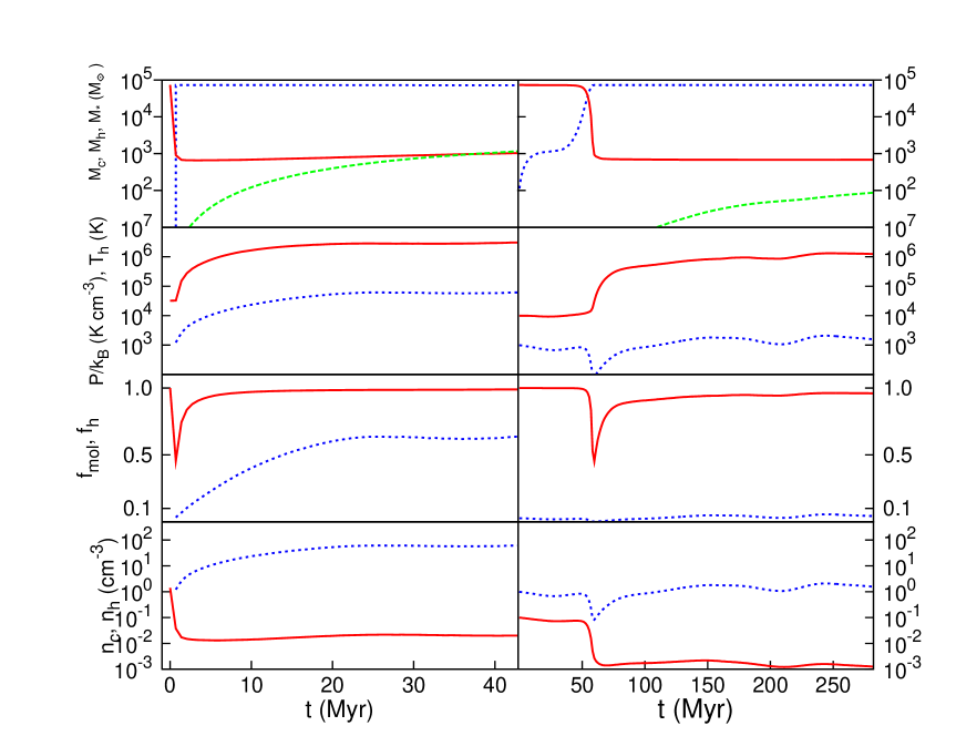
Figure 4: Evolution of ISM variables for the same two MW particles shown in Fig. 3 during one single multi-phase stage. Left panels: bulge particle, right panels: disk particle. From top to bottom: hot, cold and stellar mass gas ($M_{\rm h}$, red continuous line, $M_{\rm c}$, blue short-dashed line, $M_{\star}$, green long-dashed line); pressure $P/k_{B}$ (blue dashed line) and hot phase temperature $T_{\rm h}$ (red continuous line); molecular fraction $f_{\rm mol}$ (blue dashed line) and hot phase filling factor $f_{\rm h}$ (red continuous line); particle number densities of cold and hot phases ($n_{\rm c}$: blue dashed line; $n_{\rm h}$: red continuous line). The time is measured since the entrance of the particles in the multi-phase regime.

3.2 Evolution of multi-phase particles

A close look to the system of equations 9-11 and 15 reveals that this system, if integrated in isolation (constant average density and $\dot{E}_{\rm hydro}=0$), leads to a runaway of the molecular fraction. In fact, stellar feedback increases gas pressure, and this leads to higher molecular fraction which further increases feedback. This runaway stops when the molecular fraction saturates to unity. This instability is interrupted when the particle can exchange energy with neighbors through the hydro term $\dot{E}_{\rm hydro}$. In this case the particle starts expanding when its pressure is higher than the one of its neighbors. This gives origin to a negative $\dot{E}_{\rm hydro}$ term which cools the particle. For this reason the existence of a runaway does not imply that all particles reach very high pressure, irrespective of their environment. This fact highlights the need of an explicit integration of the system of equations, because assuming an equilibrium solution would imply on the one hand some more strong assumptions on the system (for instance, a simplified star formation law which is independent of pressure), on the other hand the transient which leads to a quasi-equilibrium solution through the pressurization of the particle would be missed.

To illustrate the behavior of the ISM as described by our sub-resolution model, we show the evolution of two MP gas particles. We use the MW initial condition, with MUPPI parameters set to the fiducial values given in Table 3. We choose two particles, whose initial positions are located at $\sim 2$ kpc (bulge particle) and $\sim 8$ kpc (disk particle) from the galaxy center, respectively. Figure 3 shows how the dynamical time of each particle, computed within each multi-phase stage, changes during 2 Gyr of evolution, starting from $\sim 1.3$ Gyr so as to avoid the initial transient during which all the gas in the MW simulation simultaneously enters in the multi-phase condition. As explained in Section 2.2, the dynamical time is kept frozen after 95 per cent of cold mass is accumulated. We note that the dynamical times scatter around values of $2\sim 10^{7}$ yr and $\sim\times 10^{8}$ yr, showing that the bulge particle has a higher evolution rate. We also note that in some cases the dynamical time of the disc particle reaches a stable value only after some tens or hundreds Myr.

Figure 4 shows for the same two particles (from top to bottom panels) and for one specific multi-phase stage, the evolution of mass of the three components ($M_{\rm c}$, $M_{\rm h}$ and $M_{\star}$), pressure $P/k_{B}$ and temperature of the hot phase $T_{\rm h}$, hot phase filling factor $f_{\rm h}$ and fraction of molecular gas in the cold phase $f_{\rm mol}$, particle number densities $n_{\rm c}$ and $n_{\rm h}$ of the two gas phases. Their evolution is followed from their entrance in multi-phase to their exit, which takes place after two dynamical times of the cold phase. These two particles have been chosen so as not to spawn a star particle before or during this cycle. For the second particle, a cycle has been chosen in which deposition of cold phase, and thus the computation of the cold phase dynamical time, does not start immediately after entrance in multi-phase.

As for the bulge particle, although initial conditions are set with all mass in the hot phase, most mass cools already during the first SPH time-step. The disc particle instead enters the multi-phase regime at a relatively low temperature and density. Therefore, due to the absence of any molecular cooling in our simulations, it has to wait until it is heated (by compression or by feedback) to high enough temperature to develop a significant cooling flow and deposit mass to the cold gas phase. In this second case, the drop in pressure visible after the onset of cooling is due to the decrease of the mean particle temperature caused by the accumulation of cold phase. Then, for both particles energy from SN explosions pressurizes the gas, without causing a pressure runaway, thanks to the hydrodynamical response of the particles to this energy input. As a result, pressure increases by more than one order of magnitude for the “bulge” particle, while the “disc” particle only recovers from the drop in pressure due to cooling. This difference in pressure reflects in very different molecular fractions. For both particles the hot phase temperature settles in the range $10^{6}$–$10^{7}$ K with its filling factor remaining high. Number densities reach values of $<10^{-2}-10^{-3}$ for the hot phase in both cases, while the cold phase number density scales with ISM pressure, being the temperature of the cold phase forced to be constant at the value $T_{\rm c}=10^{3}$K.

After the first transient, the system settles into a quasi-equilibrium state where cold gas is slowly turned into stars and ISM properties evolve quite slowly. At the end of the multi-phase stage, stellar mass amounts only to $\sim 1$ and $\sim 0.1$ per cent of the total mass, so the probability of spawning a star is low. The multi-phase stage lasts for $\sim 60$ and $\sim 250$ SPH time-steps, in the two cases. After exiting the multi-phase stage, both particles are still in high density regions, so their multi-phase variables are reset and MUPPI integration starts again. Other particles are pushed out of the disc, reach densities below the threshold value for multi-phase, become single-phase and later fall back in a galactic fountain. This happens roughly in about 3 per cent of the cases.

3.3 Global properties of the MW simulation

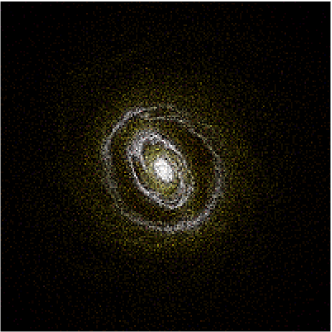
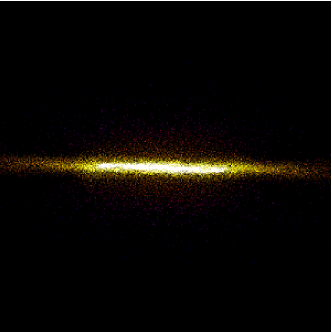
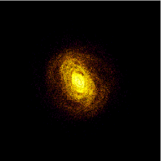
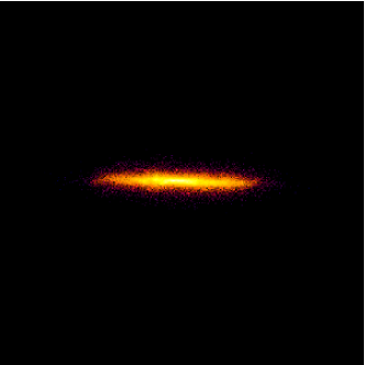
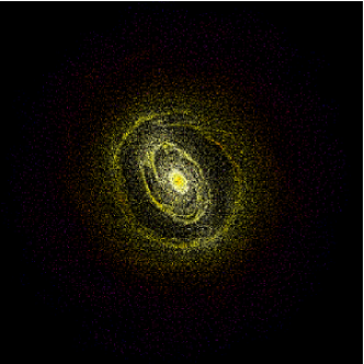
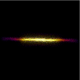
Figure 5: Distribution of gas particles (upper panels), star particles (mid panels) and SFR (lower panels) for the MW simulation with standard parameters at the end of the simulation. Particles are color coded by logarithm of their SPH density (upper and middle panels), decreasing from white to yellow to red to blue. Lower panels show again the distribution of gas particles, but the color code is the logarithm of the star formation rate. Left and right panels are for the face-on and edge-on projections, respectively. The box size is 35 kpc.

The MW simulation has been evolved for 3 Gyr. Figure 5 shows maps of gas density (upper panels), stellar mass density (central panels) and SFR (lower panels) of the MW at the end of the simulation, seen face-on and edge-on (left and right panels, respectively). In this simulation, the star formation and feedback scheme of MUPPI generates at the end of the simulation a barred galaxy with a typical spiral-like pattern, consisting of a central concentration, a star-forming circular ring at corotation, a second more distant ring and an extended gaseous disc with low molecular fraction and star formation. We remark that such a pattern is less noticeable in the first Gyrs of evolution. The edge-on view shows a characteristic of our scheme: feedback leads to a modest heating of the gas disc. We will discuss this point in more detail below.

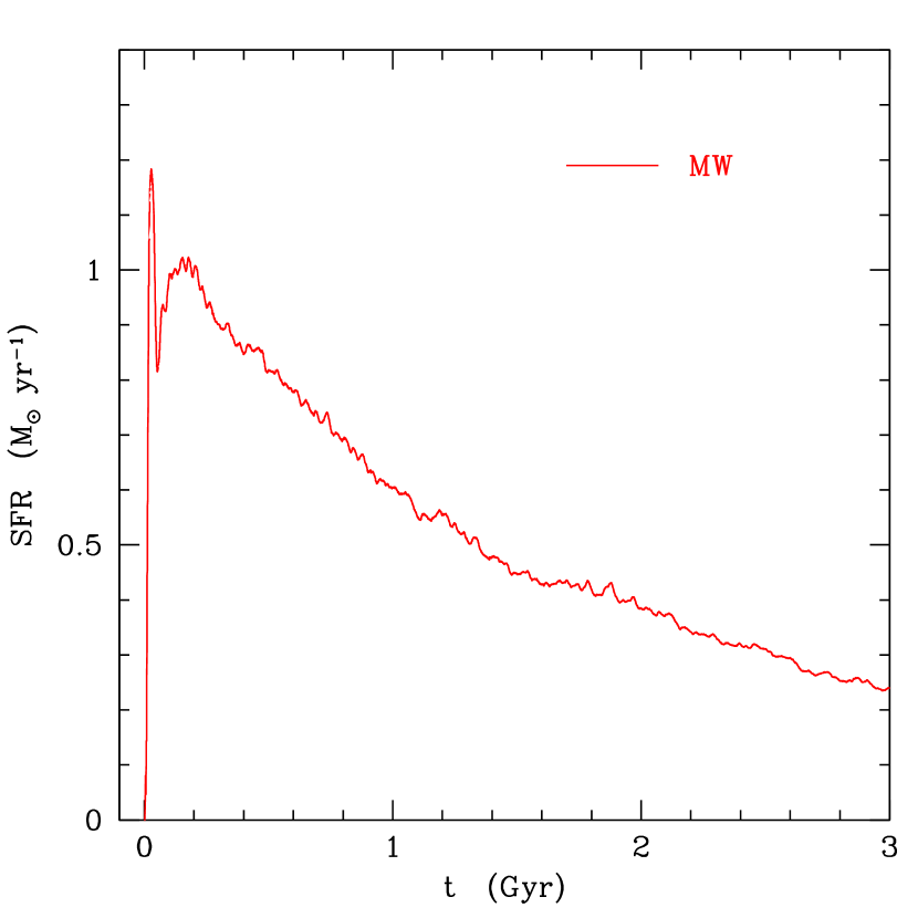
Figure 6: Star formation rate as a function of time for the MW simulation with standard parameters.

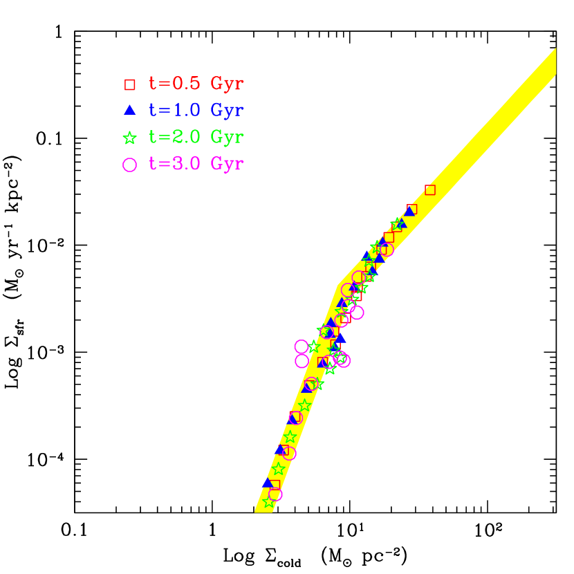
Figure 7: SK relation at four different times for the MW simulation with standard parameters, computed in concentric circles aligned with the galaxy disc. Red squares, blue triangles, green stars and magenta circles are for $t=0.5$, 1, 2 and 3 Gyr. The shaded yellow area gives a fit to the data of Kennicutt (1998) at high gas surface densities, with a break at 8 M_⊙ pc^-2 to fit the data by Bigiel et al. (2008).

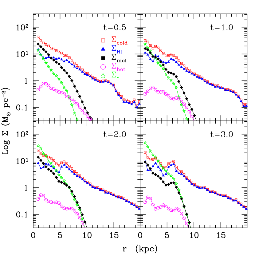
Figure 8: Surface density mass profiles of cold (red open squares), HI (blue triangles), molecular (black filled squares), hot gas (magenta circles) and (newly formed) stellar mass (green stars) for the MW simulation with standard parameters, at four different times as indicated in the panels.

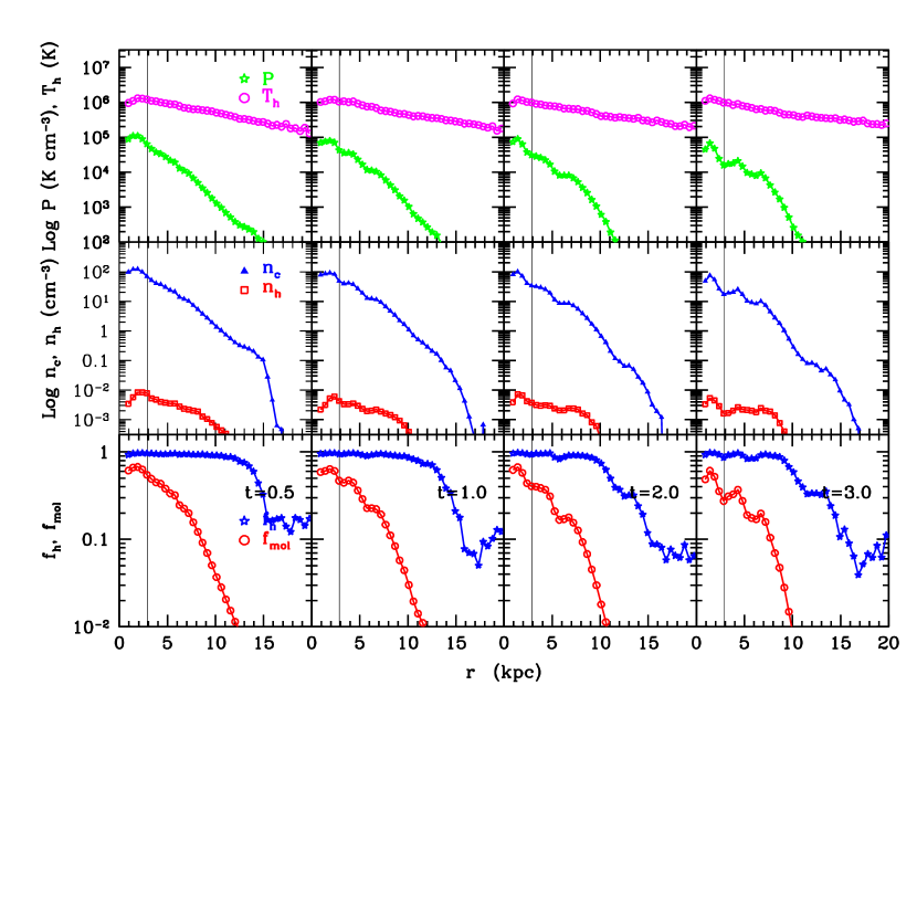
Figure 9: Average properties of the ISM as a function of radius for the MW simulation with standard parameters at four different times as indicated in the panels. Upper panels: pressure (green stars) and temperature (magenta circles) of the hot phase; central panels: number densities of the cold and hot phases (blue triangles and red squares, respectively); lower panels: fraction of hot and molecular gas (blue stars and red circles, respectively). The black vertical line marks the scale radius of our MW disk.

Figure 6 shows the total star formation rate of the galaxy. The first peak, reaching values of nearly 1.2 M_⊙ yr^-1 and lasting for a few tens of Myr, is a numerical transient due to the fact that many particles are cold and satisfy the star formation criterion already in the initial conditions. For this reason, they are out of the equilibrium when MUPPI is switched on, so that they all start forming stars at the same time, and their feedback tends to quench star formation. The second, broader peak marks the pressurization of the galaxy disk and the start of the quasi-equilibrium star-forming phase. The star formation rate then declines on a time-scale of $\sim 2$ Gyr, as expected for a disc which obeys the SK relation (see Leroy et al., 2008) and receives no mass inflow from the outside.

Figure 7 shows the comparison between the observed and the predicted SK relation, i.e. the relation between surface density of star formation rate, $\Sigma_{\rm sfr}$, and total surface gas density $\Sigma_{\rm cold}$, at four different times (0.5, 1, 2 and 3 Gyr). As we will discuss extensively in Section 3.6, this relation is actually used to tune the parameters of our model. The interpretation of this relation will be the subject of a forthcoming paper, while we focus here only on the main numerical aspects of this comparison. The shaded area shows a double power-law fit to observational data, with slope and normalization as proposed by Kennicutt (1998a) for surface densities higher than 8 M_⊙ pc^-2, and slope 3.5 for lower gas surface densities, roughly consistent with the break reported by Bigiel et al. (2008). The width of this area is compatible with the error on the zero point quoted by Kennicutt (1998a), and should not be taken as indicative of the total observational uncertainty, which is larger. Observed gas surface densities, corresponding to $HI+H_{2}$, have been corrected by a factor 1.31 to take into account the presence of helium. Quite clearly, the simulated relation is remarkably stable with time and agrees well with the observational fit. The simulated SK relation at $t=3.0$ Gyr of evolution shows a higher degree of scatter, caused by the development of the structure in the gas distribution shown in Figure 5.

Figure 8 shows the mass surface densities of cold, molecular, $HI$ (defined as $(1-f_{\rm mol})M_{\rm c}$) and hot gas, along with the SFR surface density. While $HI$ gas density flattens at $\sim 8$ M_⊙ pc^-2, molecular and stellar surface densities have comparable scale lengths. This is again in line with the observations of the THINGS group Bigiel et al. (2008); Leroy et al. (2008). The hot gas density remains at $\sim 1$ per cent of that of cold gas (here and in the following we neglect “hot” gas in particles that have not started to cool and pressurize). The pattern in the gas distribution is here visible as bumps in the density profile, which develop at later times ($t\ga 1$ Gyr).

Figure 9 shows the predicted (mass-weighted) average values of ISM properties, namely pressure and hot phase temperature (upper panels), number densities of cold and hot phases (central panels), molecular fraction and hot phase filling factor (lower panels), computed in cylindric volumes around the galaxy center of mass, as a function of radius. All profiles are computed only over MP particles. We note that pressure and hot phase temperature both follow an exponential profile, but the latter quantity is remarkably flatter. The same trend is noticeable also for the cold and hot gas number densities. The molecular fraction is high at the galaxy center but quickly decreases beyond $\sim$6 kpc, i.e. where the gas surface density drops below 10 M_⊙ pc^-2, while the hot phase filling factor is very high throughout the region where star formation is present.

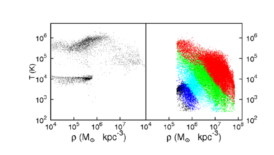
Figure 10: Phase diagram for particles in the MW simulation with standard parameters, after 2 Gyr. Left and right panels show respectively single- and MP particles. The latters are color-coded according to their SFR as follows (all SFRs being in M_⊙ yr^-1). Black: $[0,10^{-8})$; blue: $[10^{-8},10^{-7})$; cyan: $[10^{-7},10^{-6})$; green: $[10^{-6},10^{-5})$; red: $>10^{-5}$.

Figure 10 shows the density–temperature phase diagram for single-phase (left panel) and MP (right panel) gas particles after 2 Gyr of evolution. Mass-averaged temperature and SPH gas density are shown for the MP particles. At low densities, most single-phase particles lie in two sequences at temperature $\sim 10^{4}$ and $\sim 5\times 10^{5}$ K respectively. They correspond to cold particles lying on the disc and to particles heated by thermal feedback. Some single-phase particles reside above the density threshold. These are particles that have exited the multi-phase stage at high average temperature and can not re-enter it immediately after. The multi-phase sequence starts with a drop in temperature, which corresponds to the initial accumulation of cold mass lowering the average temperature. The bump at $T\sim 10^{5}$ K corresponds to the pressurized and star-forming particles with $T_{\rm h}\sim 10^{6}-10^{7}$ K and hot mass fraction of $\sim 1$ per cent. Two denser regions in the MP particle phase diagram, at densities $\rho\sim 10^{7}$ and $\sim 3\cdot 10^{7}$ M_⊙ kpc^-3 corresponds to regions of the galaxy where density is enhanced by spiral arms.

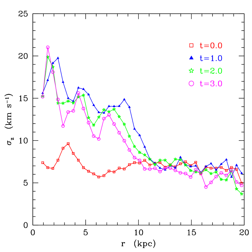
Figure 11: Profiles of r.m.s. vertical velocity as a function of radius for the MW simulation at four different times, including the initial conditions corresponding to $t=0$.

Figure 11 shows the profiles of the r.m.s. value of the vertical velocity, $\sigma_{z}$, for gas particles in the initial conditions and at three different times. As already noticed from the edge-on view of the gas disc in Fig. 5, feedback leads to a thickening of the disc, which is visible here as an increase of the vertical velocity from $\sim 7$ km s^-1 to a peak value of $\sim 20$ km s^-1 in the inner kpc. These values are in line with, though on the high side of, the observational determination of Tamburro et al. (2009) based on THINGS 21-cm data.

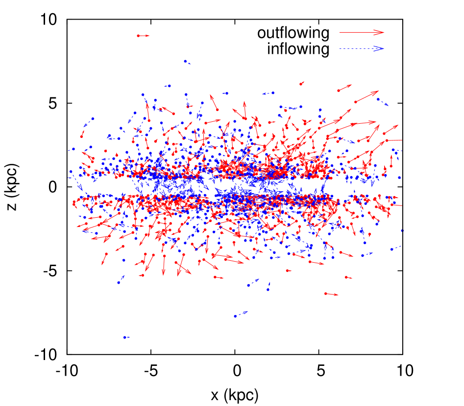
Figure 12: Particle velocities above and below the disc for the MW simulation after 1 Gyr. Gas particles with $|y|<0.5$ kpc are shown in the xz-plane; particles with $|z|<0.5$ kpc are removed for sake of clarity. Red (continuous) and blue (dashed) particles are respectively outflowing and inflowing ones. Vector lengths are scaled with velocity, 1 kpc corresponding to 50 km s^-1.

The edge-on images of Figure 5 show that the disc is surrounded by a thick corona of gas particles. Figure 12 shows velocities for such corona particles at $t=1$ Gyr; only a slice with $|y|<0.5$ kpc is shown, and particles with $|z|<0.5$ kpc are removed for sake of clarity. Outflowing and inflowing particles are shown with different colors and line styles, vector lengths are scaled with velocity, 1 kpc corresponding to 50 km s^-1. This figure shows that such particles are ejected from the disc with modest velocities, reaching values of about 50 km s^-1, in agreement with, e.g., Spitoni et al. (2008), and falling back in a fountain-like fashion. We computed the resulting outward and inward mass flows that cross the planes located 1 kpc above and below the disk midplane. We verified that they are nearly equal at all radii and their values integrated along the radius are similar to the average SFR.

From the results shown in this section, we conclude that MUPPI provides a realistic description of the ISM of a Milky Way-like galaxy. The hot phase has negligible mass but high filling factor, and its properties are relatively stable with radius and time. Cold non-molecular ($HI$) gas surface density roughly flattens at $5-8$ M_⊙ pc^-2, while molecular gas dominates in the internal parts of the galaxy. From the one hand, this is a consequence of an exponential pressure profile, with a molecular fraction scaling with pressure as in equation 5. On the other hand, pressure results from the interplay of an intrinsically unstable system, which would tend to a pressure runaway up to saturation of the molecular fraction, and the hydrodynamical feedback of this system on the surrounding gas.

3.4 Global properties of the DW simulation

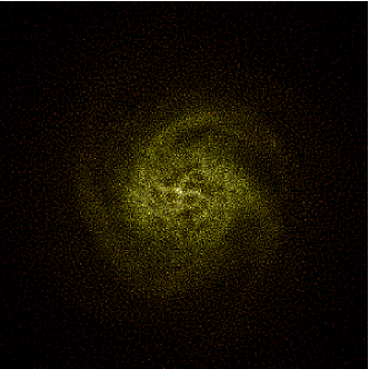
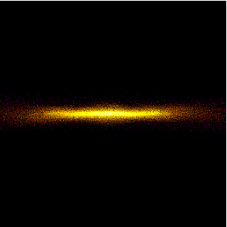
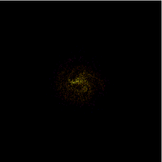
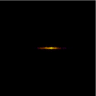
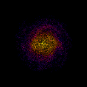
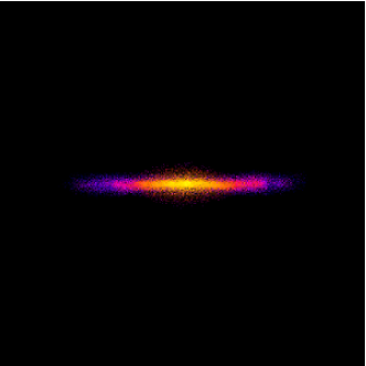
Figure 13: Distribution of gas particles (upper panels), star particles (mid panels) and SFR (lower panels) for the DW simulation with standard parameters after 3 Gyr. The color code is the same as in Figure 5, but we took lower maximum values for SFR and stellar density to enhance the color contrast. The box size is 35 kpc.

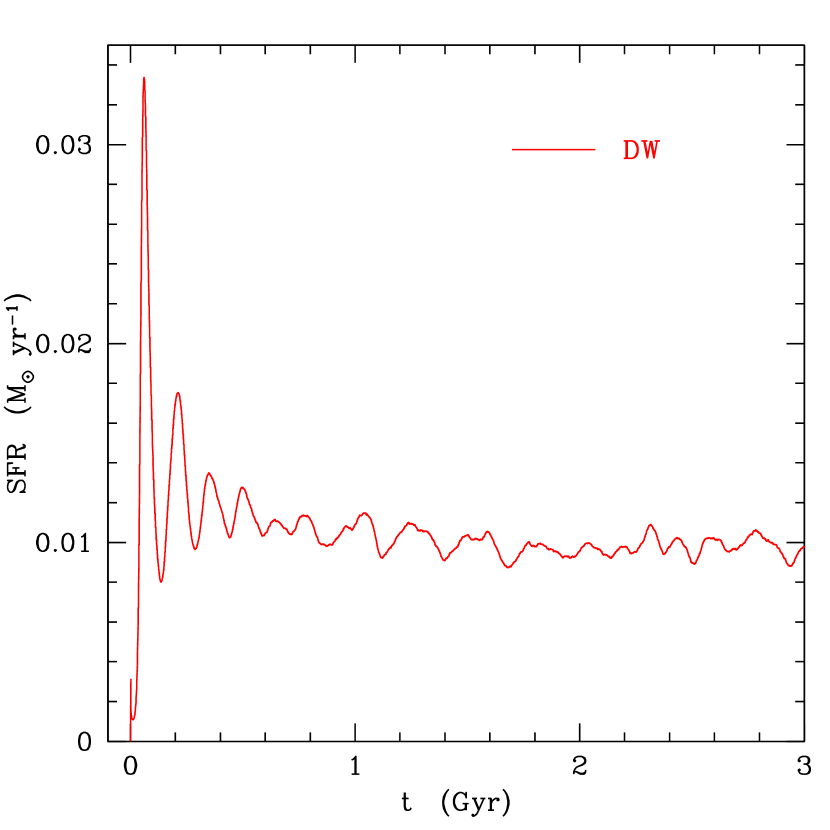
Figure 14: Star formation rate as a function of time for the DW simulation with standard parameters.

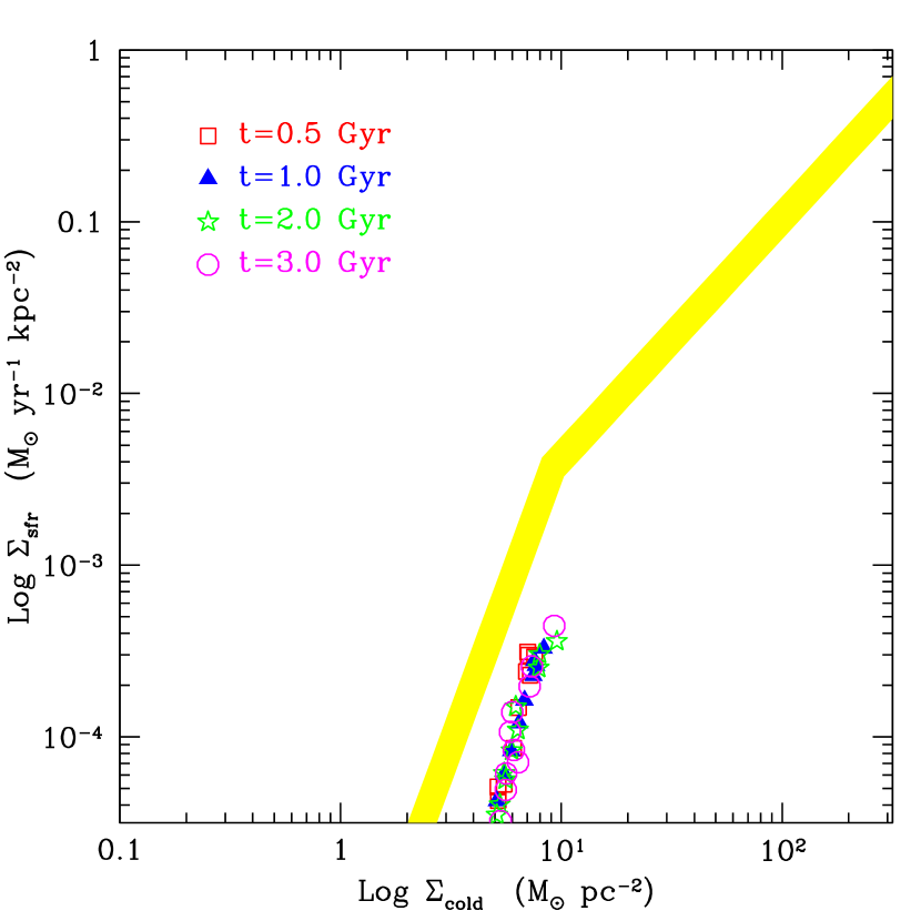
Figure 15: The same as Figure 7, but for the simulation of the DW galaxy.

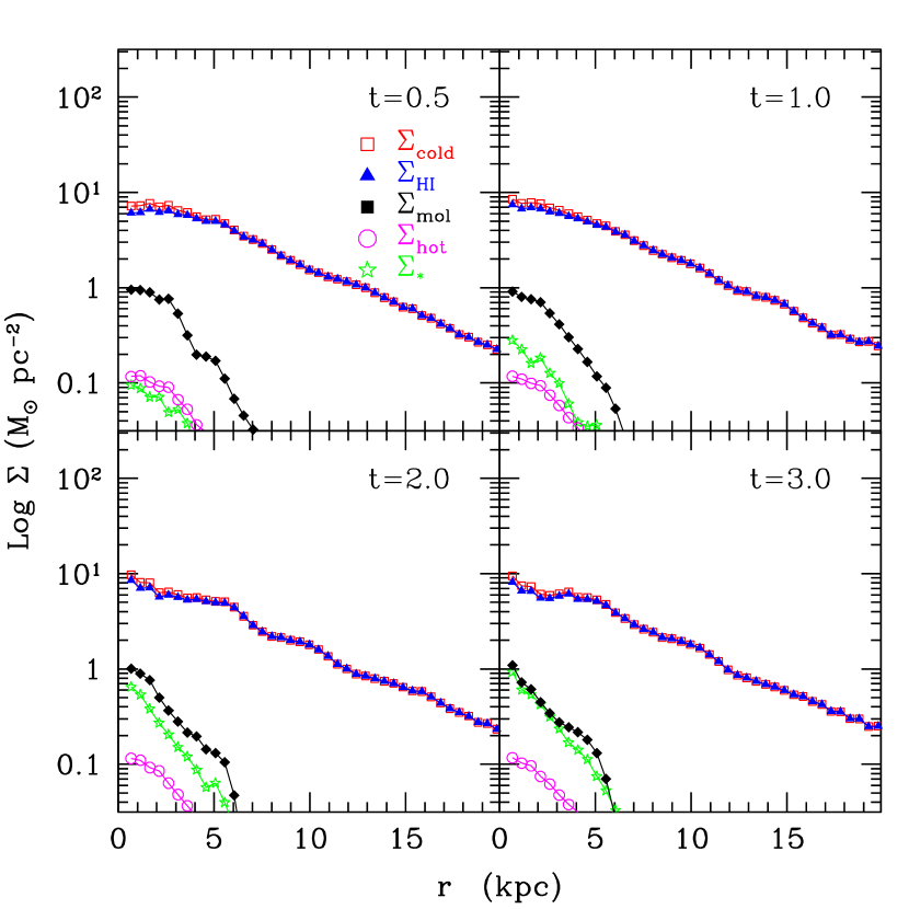
Figure 16: The same as Figure 8 but for the simulation of the DW galaxy.

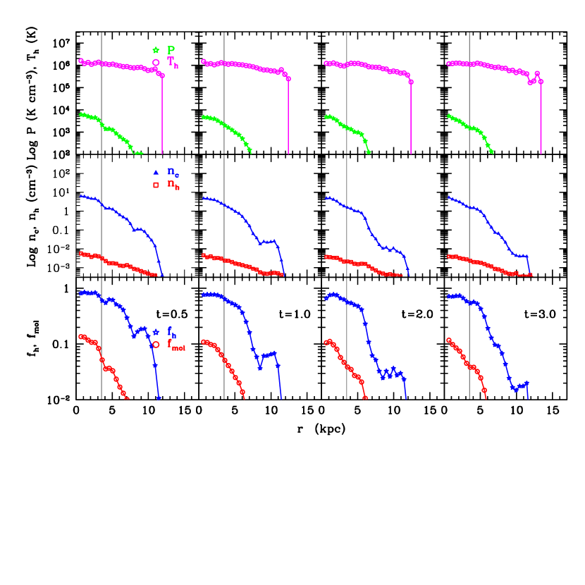
Figure 17: The same as in Figure 9, but for the simulation of the DW galaxy. Here, the black vertical line marks the scale radius of our DW disk.

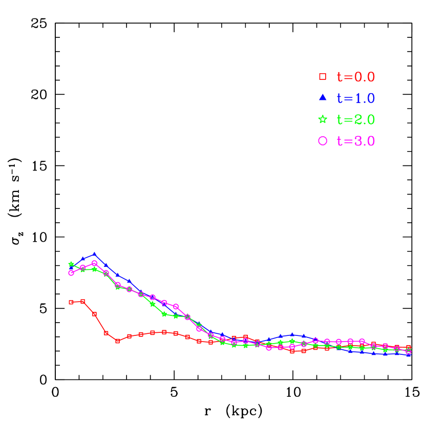
Figure 18: The same as in Figure 11, but for the simulation of the DW galaxy.

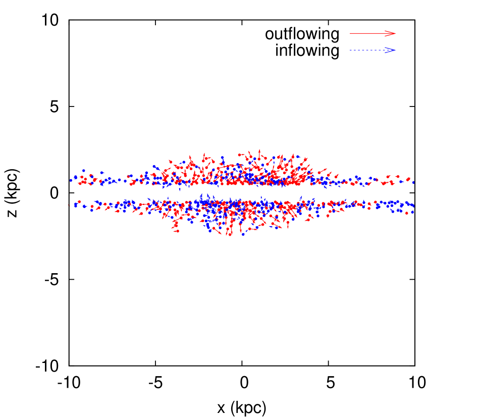
Figure 19: The same as in Figure 12, but for the simulation of the DW galaxy.

As for the simulation of the DW galaxy, Figure 13 shows gas, star density and SFR maps at the end of the simulation, while Figures 14, 15, 16, 17, 18 and 19 show SFR, SK relation, surface density profiles, ISM properties, vertical velocities and particle velocities above or below the disc. The gas surface density of this galaxy is low, reaching values of $\sim 10$ M_⊙ pc^-2 only at the very center. The molecular content of the galaxy is thus small, and the SFR proceeds at the rate of $\sim$0.01 M_⊙ yr^-1, mildly declining with time. The transition to MUPPI dynamics causes oscillations of period $\sim 100$ Myr, that are slowly damped during the evolution. Unlike for the MW case, the SK relation is now below the observational estimate, is steep and slightly displaced with respect to that of the external regions of the MW, but preserves the stability with evolution. Pressure and molecular fraction are always low, so the galaxy is dominated by $HI$ gas. Hot phase temperature is again the most stable quantity, it stays around $10^{6}$ K up to $\sim 12$ kpc, where the SFR drops to very low value; hot gas number and mass surface densities are lower than for the MW case. Vertical velocities are also lower than the MW counterpart. The spiral pattern is hardly visible in the stellar component but more apparent in the gas component, where the flocculent morphology in the center is reminiscent of the $HI$ holes seen in nearby dwarf galaxies. Outflowing velocities are lower than for the MW case, but the extent of the corona generated by the fountain is a few kpc, thus indicating that the shallower potential well allows gas particles to be ejected to similar heights despite the fact that they receive a much lower energy input.

These differences with respect to the MW simulation are in line with the observational evidence (Bigiel et al., 2008; Leroy et al., 2008; Tamburro et al., 2009) of dwarf galaxies being morphologically irregular, $HI$-dominated, with very small values of star formation and vertical velocity, and a steep SK relation roughly coinciding (but slightly displaced) with respect to that of the external parts of normal disc galaxies.

3.5 Non–rotating halos

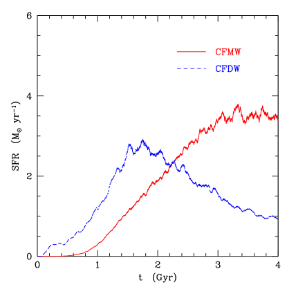
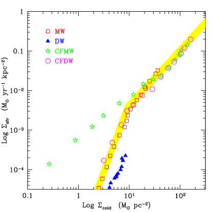
Figure 20: Evolution of the star formation rate (left panel) and SK relation after 2.78 Gyr of evolution (right panel) for the simulations of the Milky Way and dwarf non–rotating halos (CFMW and CFDW runs, respectively). Also shown for reference in the right panel are data points from the results of the SK relation for the rotating MW and DW simulations after 278 Myr.

The main reason to test MUPPI on spherical, non-rotating, isolated cooling flow halos is that this configuration leads to a galaxy with a geometry which is completely different from that of a rotating disc. In this case we can directly test whether the implemented scheme of energy redistribution causes a different behavior of feedback in different geometries. In Figure 20 we show the SFR (left panel) and the SK relation after 2.78 Gyr (right panel), for the Milky Way (CFMW) and dwarf (CFDW); for reference we also report data points from the SK relation for the rotating MW and DW simulated galaxies, shown at a relatively early time (278 Myr) to probe the relation at higher surface densities. The SFRs show an initial rise due to the onset of the cooling flow, a peak and then, for the CFDW case, a decrease, while the CFMW curve is flat down to 4 Gyr. The difference in the onset of cooling is due to the different virial temperature of gas in the initial conditions and thus to the different cooling times of the halos. Moreover, the concentration of our CFDW halo is higher than that of the CFMW. For these reasons, in the central region the cooling time is shorter and star formation starts earlier. The peak is mainly determined by feedback, which pressurize the multi-phase gas and enhance its SFR.. The more massive halo peaks at higher values as expected from its higher mass and deeper potential well.

We show the SK relation at the latest output of our CFDW run. The two cooling flows reach much higher surface densities than the isolated discs. The CFDW simulation is very similar to the MW at low gas surface densities, but drops below the MW result at $\sim 30$ M_⊙ pc^-2, while steepening at higher densities. The CFMW has a more peculiar behavior: it stays well below the observed relation at high gas surface density, then converging to the CFDW simulation (and below the MW one) at higher densities. The first point highlighted by this test is that the SK relation is not trivially fixed by the model, instead it is obtained, although after a suitable choice of model parameters, only in the case of a thin rotating disc. At high densities, the SK relation of cooling flows tends to stay at the lower boundary allowed by the observed relations, as shown in Figure 20, and below the SK relation of the the MW simulation. As we will discuss in the following, the latter tends to steepen at higher resolution, while the two cooling flow simulations show a remarkable stability against mass and force resolution. This result can be explained as follows: in a thin system, like the MW disc, energy is deposited preferentially along the vertical direction. Therefore, particles that receive most energy are those that stay just above or below the disk midplane. This causes the fountain-like flow described above and allows mid-plane particles to remain cold and dense. In the spherically-symmetric system this does not happen. In this case, energy is injected much more effectively in the gas particles, so that these are much more pressurized. At the same time, such particles expand more and, compared with regions with similar gas surface density in the disk midplane, they achieve lower densities.

The SK relation of the CFMW simulation at low surface densities is more surprising. Due to the higher virial temperature and longer cooling time of the hot gas initially present in this halo, single-phase particles flowing toward the center are hot and thus not eligible to enter in the multi-phase regime. As a consequence, MP particles outflowing from the central star-forming region are surrounded by hot particles that pressurize them but, being hot, cannot contribute to the cold gas surface density. Indeed, if all gas particles are (incorrectly) included in the calculation of the gas surface densities, the other SK relations are moved to the right by a small amount, while the SK relation of the CFMW run is shifted slightly below the observed one at all surface densities. In a realistic case, this mechanism could be relevant for weak star formation episodes taking place outside the main body of large galaxies, like in winds or tidal tails embedded in a hot rarified medium.

3.6 Fixing the parameters

We performed a number of test runs to control the behavior of our model as we vary its parameters, and to determine our reference set of parameters. Some of them influence the model in a quite predictable way, so we will only briefly discuss them and concentrate in the following on those that need a more detailed discussion. Unless otherwise stated, we use the isolated MW initial conditions to carry out our tests.

The full set of MUPPI parameters, shown in Table 3 amounts to 8 values: $f_{\star}$, $P_{0}$, $T_{\rm c}$, $f_{\rm fb,out}$, $f_{\rm fb,local}$, $f_{\rm ev}$, $\theta$.

To these we should add two parameters that are set by stellar evolution and choice of the IMF, namely $E_{\rm SN}/M_{\star,\rm SN}$, which is set to $10^{51}\ {\rm erg}/120\ {\rm M}_{\odot}$ (and is degenerate with $f_{\rm fb,out}$ and $f_{\rm fb,local}$), and the restoration factor $f_{\rm re}=0.2$. Moreover, the model has two thresholds $n_{\rm thr}$, $T_{\rm thr}$, which sets the minimum values of density and temperature for gas particles to enter in the multi-phase stage, and two exit conditions $n_{\rm out}$, $t_{\rm clock}$.

The diagnostic that we use to quantify the influence of parameter variations on simulation results are the SFRs and the SK relation. The latter has good observational constraints as far as slope, normalization and low-density cut-off are concerned. When we vary a parameter, we keep all the others fixed to our “reference” values (see Table 3).

Figure 21 shows the behavior of our simulated SFR and SK relation when we vary the star formation efficiency $f_{\star}$. We used $f_{\star}=0.01$,$0.02$, $0.05$. This parameter influences the normalization of the SK relation in a straightforward way. Indeed, this relation fixes the consumption time-scale of cold gas into stars, $M_{\rm c}/\dot{M}_{\star}$, which is regulated by $f_{\star}$ through equation 4. We notice that the value $f_{\star}=0.02$, corresponding to 2 per cent of a molecular cloud being transformed into stars before being disrupted by stellar feedback, is well in line with observations (see, e.g., Krumholz & Tan, 2007).

As for the effect of $P_{0}$, it enters the model only through $f_{\rm mol}$, which is multiplied by $f_{\star}$ in equation 4. As a consequence, the two parameters $P_{0}$ and $f_{\star}$ are degenerate. However, since the relation is non-linear, we carried out a test obtained by varying $P_{0}/k$, with respect to the observational value given by Blitz & Rosolowsky (2006), to 20000 and 50000 K cm^-3. The results of this test are shown in Figure 22. We find that the implied variation of the final results is smaller than that caused by changing the other parameters. The SK relation is remarkably stable against changes in $P_{0}$; only low values of such parameters result in too high a $\Sigma_{\rm sfr}$ for a given $\Sigma_{\rm cold}$. Straightforwardly, an higher $P_{0}$ gives a lower SFR.

Due to the condition of pressure equilibrium ($P/k=n_{\rm c}T_{\rm c}$), the value of $T_{\rm c}$ fixes the proportionality between cold gas density, directly related to dynamical time $t_{\rm dyn}$, and SPH pressure. The lower this value is, the fastest the evolution of a MUPPI particle. The chosen reference value, $T_{\rm c}=10^{3}$K, is similar to that used in literature for other star formation and feedback schemes (e.g., Springel & Hernquist, 2003). We tested that lowering it to $T_{\rm c}=100$ (as, e.g., in M04) turns into very short dynamical times and very fast evolution for our MUPPI particles, corresponding to high star formation rates, which must then be compensated by a very low, possibly unrealistic, value of $f_{\star}$.

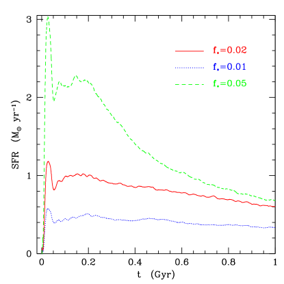
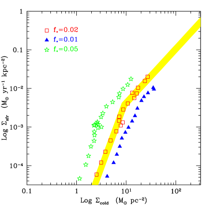
Figure 21: Effect of varying $f_{\star}$ on the evolution of star formation rate (left panel) and SK relation after 1 Gyr (right panel) for the MW simulation. Dashed curve and stars (in green), solid curve and squares (in red), dotted curve and triangles (in blue) correspond to $f_{\star}=0.05$, 0.02 and 0.01, respectively. The shaded area has the same meaning as in Fig. 7.

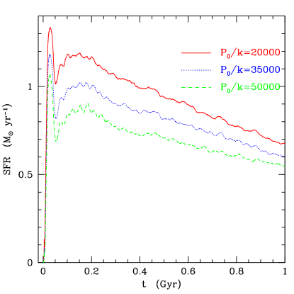
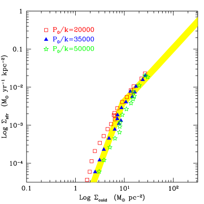
Figure 22: The same as in Figure 21, but for the effect of varying the $P_{0}$ parameter. Short-dashed curve and stars (in green), dotted curve and triangles (in blue), solid curve and squares (in red) correspond to $P_{0}/k=50000$, 35000 and 20000 K cm^-3, respectively.

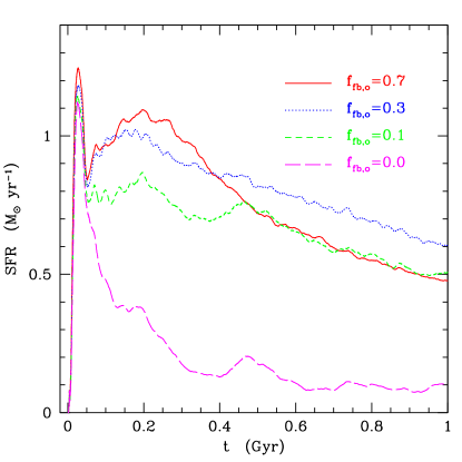
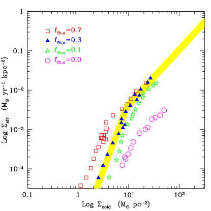
Figure 23: The same as in Figure 21, but for the effect of varying the $f_{\rm fb,out}$ parameter. Long-dashed curve and circles (in magenta), short-dashed curve and stars (in green), dotted curve and triangles (in blue), solid curve and squares (in red) correspond to $f_{\rm fb,out}=0$, 0.1, 0.3 and 0.7, respectively.

Figure 23 shows the effect of varying the value of the parameter $f_{\rm fb,out}$, which regulates the amount of SN energy transferred to neighboring gas particles. We used the values 0, 0.1, 0.3 and 0.7. The SFR increases when this parameter ranges from 0 to 0.3. This is due to the fact that gas particles receiving more energy are more pressurized and produce more stars. In particular, a relatively high value of $f_{\rm fb,out}$ is needed to pressurize gas particles and sustain star formation, at least with the adopted choice of $f_{\rm fb,local}$. We checked that ISM variables (temperature, numerical density of hot and cold gas) all increase correspondingly. When $f_{\rm fb,out}$ further increases, another effect takes over: a larger amount of gas is ejected from the disk, thus becoming unavailable for star formation, with a subsequent decrease of the cold gas mass fraction. As a consequence, the SFR begins to decrease too. Apart from the extreme case $f_{\rm fb,out}=0.0$, at large values of $\Sigma_{\rm cold}$ the simulated SK relation always stays within the observational limits. The effect of a stronger feedback is however to decrease the value of the surface density at which the SK relation begins to sharply decline, thus tuning the position of the break in the SK relation. With $f_{\rm fb,out}=0.3$ we obtain fair agreement with observations by Bigiel et al. (2008). Therefore we choose this value as the reference one.

Properties of the ISM, SFR and SK relation are all largely insensitive to the exact value of $f_{\rm fb,local}$, as far as it is smaller than $f_{\rm fb,out}$. Keeping all the other parameters fixed, a vanishing value of $f_{\rm fb,local}$ would lead to an increase in the number of particles that exit the multi-phase regime because of catastrophic loss of hot phase thermal energy. For this reason we preferred the small value $f_{\rm fb,local}=0.02$, although it is insufficient to pressurize particles in the absence of outward distributed energy.

The amounts of cold gas evaporated by SNe, $f_{\rm ev}$, has been fixed to 0.1 following the suggestion of M04 and Monaco (2004a) that the main evaporation channel is due to the destruction of the star-forming cloud, most of which is snow-ploughed back to the cold phase.

Varying the angle $\theta$ or the distribution scheme of the energy to neighboring particles does not introduce significant differences in the global behavior of SFR and SK relation, while it changes the morphology of the galaxy. We show in Figure 24 the gas distribution seen face-on after 1 Gyr in four cases, $\theta=30^{\circ}$, $\theta=60^{\circ}$ (the standard case), $\theta=60^{\circ}$ with energy not weighted by the distance from the axis but only by the distance from the particle, and the case of isotropic distribution of energy. Clearly the spiral pattern in the gas distribution weakens when moving from the first to the last case. For instance, an isotropic distribution of energy leads to the complete disappearance of the spiral pattern. Our preference for the wider opening angle, $\theta=60^{\circ}$, is motivated as follows: with a narrower angle it frequently happens that particles have no neighbors in the direction of decreasing density, thus leading to a loss of the outflowing energy. Figure 25 shows the resulting velocities of particles above or below the disc (see Fig. 12 for the standard MW case): distributing energy more selectively, i.e. within a smaller aperture angle, creates a more pronounced fountain.

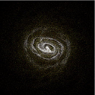
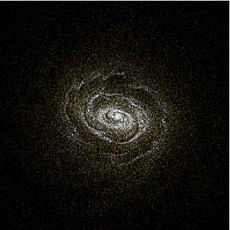
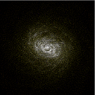
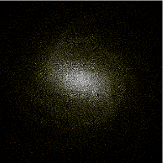
Figure 24: Density maps of gas for the MW simulation after 1 Gyr for four cases obtained by changing the prescription to distribute feedback energy: $\theta=30^{\circ}$ (upper left), the standard case $\theta=60^{\circ}$ (upper right), $\theta=60^{\circ}$ with energy not weighted by the distance from the axis but only by the distance from the particle (lower left), isotropic distribution of energy (lower right). The color code is as in Fig. 5.

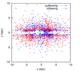
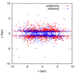
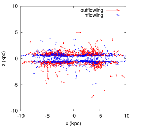
Figure 25: Particle velocities as in figure 12, for the MW simulation after 1 Gyr for three cases: $\theta=30^{\circ}$ (left), $\theta=60^{\circ}$ with energy weighted by the distance from the particle (middle), and for an isotropic distribution of energy (right).

As for the conditions for the onset of the multi-phase regime, we verified that they have no strong influence on the simulations of isolated galaxies like those presented here. This holds at least as long as the threshold density $n_{\rm thr}$ is kept low and the temperature threshold lies in the instability range below $10^{5}$ K, that is not populated by single-phase particles (see Figure 10). This result may not necessarily hold in the case of cosmological initial conditions. This specific point will be addressed in a forthcoming work. As far as the exit conditions are concerned, we adopted a value of $n_{\rm out}$ slightly lower than $n_{\rm thr}$ to avoid the case of particles rapidly bouncing between multi- and single-phase regimes. Finally, our chosen value for $t_{\rm clock}$ is suggested by theoretical reasons (see Section 2.2). We tested the effect of taking higher values for $t_{\rm clock}/t_{\rm dyn}$ and found that a large amount of stars is produced outside the disk, because pressurized and blowing-out particles stay multi-phase even when their density is rather low. This feature is not desirable, thus giving further justification to the low value adopted for this parameter.

3.7 Effect of resolution

In order to test the sensitivity of MUPPI to resolution, we run the same MW simulation with mass resolution 10 times worse (LR) and 4.62 times better (HR), and force resolution (scaled as the cubic root of the mass resolution) $\simeq 2.2$ times larger and $\simeq 1.7$ times smaller, respectively. The expensive HR simulation was stopped after 500 Myr, so we make our comparison at this time, which is after the first (transient) peak of star formation. Figure 26 shows SFRs, SK relations, surface density profiles and vertical velocity dispersions for the three runs. The three vertical dotted lines in the plot of the density profile mark three times the softening for the three runs. From these plots it is clear that the poor resolution of the LR run does not allow to resolve the inner part of the disc, where most mass is located. This results in a low normalization of the SK relation and high velocity dispersion of clouds, i.e. a thicker gas disc. Increasing the mass resolution by $\sim 45$ times, from the LR to the HR run, improves the description of the disc at smaller radii. In turn, this provides a reasonable degree of convergence in density profiles, velocity dispersion and in the SK relation, beyond three softening lengths. In particular, we note that total, atomic and molecular gas surface density profiles are stable when resolution is changed. However, this does not correspond to a convergence of the SFR, and consequently of the stellar surface density profiles, that keeps increasing as long as the inner regions give an important contribution. Indeed, we notice that at $t=0.5$ Gyr the level of SFR increases by about almost a factor 3 as we increase mass resolution by about a factor 45 from the LR to the HR run.

As a conclusion, the results of our sub-resolution model show in general a mild dependence on numerical resolution. This dependence is more pronounced for the SFR, owing to the fact that the bulk of star formation takes place within the very central part of the galaxy. We consider this as an undesired characteristic of the model. On the other hand, it is worth pointing out that one of the mayor advantages of our sub-resolution model lies in the fact that ISM properties are determined by the local hydrodynamical characteristics of the ambient gas (which are obviously resolution-dependent), respond to its changes, and provide an effective feedback to it. This is a focal difference with respect to, for instance, the multi-phase effective model by Springel & Hernquist (2003).

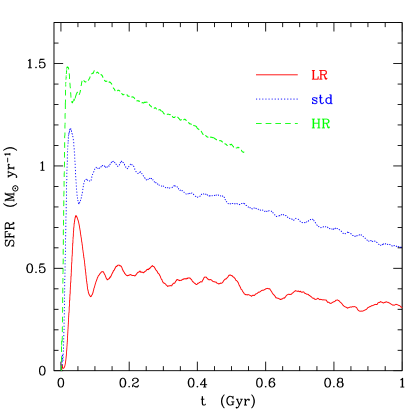
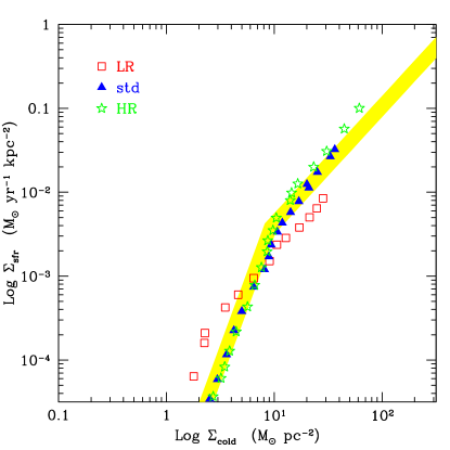
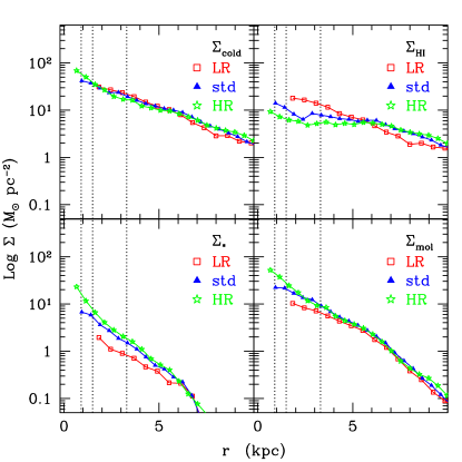
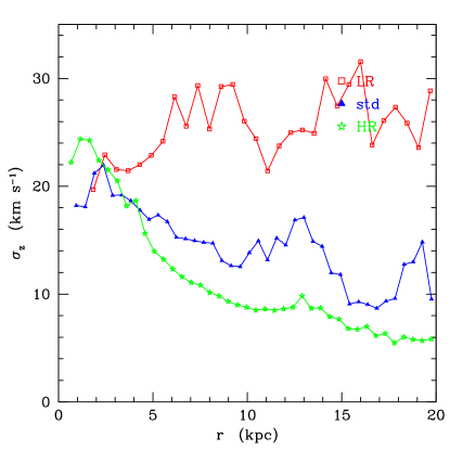
Figure 26: Stability of results of the isolated MW simulation against numerical resolution. Star formation rate, SK relation, surface density profiles of ISM properties and profiles of the r.m.s. vertical velocity are shown from the upper left to the bottom right panel. In the bottom left panel, vertical lines mark the force resolution (i.e., three times the plummer-equivalent gravitational softening) of our three simulations. All results, except those in the upper left panel, refer to 100 Myr of evolution.

4 Conclusions

We presented MUPPI (MUlti-Phase Particle Integrator), a new sub-resolution model for stellar feedback in SPH simulations of galaxy formation, developed within the GADGET-2 code. The code is based on a version of the model of star formation and feedback developed by (Monaco, 2004b) (M04), which has been modified and greatly simplified to ease the implementation in a code for hydrodynamic simulations. In this model, each SPH gas particle is treated as a multi-phase system with cold and hot gas in thermal pressure equilibrium, and a stellar component. Cooling of MP particles is computed on the basis of the density of the diluted hot phase, which carries only a small fraction of the mass but has a very high filling factor. Energy generated by SNe is distributed mostly to neighboring particles, preferentially along the “least resistance path”, as determined by the gradient of local density field. This allows different feedback regimes to develop in different geometries: in a thin disc energy is injected preferentially along the vertical direction, thus creating a galactic fountain while the disc is heated to an acceptable level; in a spheroidal configuration energy is trapped within the system and feedback is more efficient in suppressing star formation.

One of the main ingredients of the model is the use of the phenomenological relation of Blitz & Rosolowsky (2004, 2006), which connects the fraction of molecular gas with the external pressure of the star-forming disc. Using this relation with SPH pressure results in a system of equations that gives rise to a runaway of star formation. Indeed, SN energy increases pressure, and this leads to a higher molecular fraction which turns into more star formation, up to the saturation of the molecular fraction. This runaway does not take place as long as the hydrodynamical response of the particle leads to a decrease of pressure. The consequence of this is that thermal feedback alone is efficient in regulating star formation in an SPH simulation. This is uncommon in many sub-resolution models of star formation and feedback currently implemented in numerical simulations.

We tested our code with a set of initial conditions, including two isolated disc galaxies and two spherical cooling flows. These tests show the ability of the code to predict the slope of the SK relation (Kennicutt, 1998b; Bigiel et al., 2008) for disc galaxies, the basic properties of the inter-stellar medium (ISM) in disc galaxies, the surface densities of cold and molecular gas, of stars and SFR, the vertical velocity dispersion of cold clouds and the flows connected to the galactic fountains. Self-regulation of star formation does not result in a bursty or intermittent SFR, though the DW galaxy shows damped oscillations in the first Gyr. This is because the intrinsically unstable behavior of gas particles is stabilized by the SPH interaction with the surrounding particles. In the global SFR, we average over all the MP particles and thus smooth the intermittent behavior of particles and creates a more stationary configuration with a slowly declining SFR.

Furthermore, the cooling flow simulations show the dependence of feedback on the geometry of the star-forming galaxies. On the one hand, these simulations show that MUPPI does not trivially fix the SK relation, which is in fact reproduced only in the case of a thin rotating discs. On the other hand, the difference we obtain in the SK relation for our cooling flows shows that the geometry influences the behavior of our model, correctly distinguishing a thin system from a thick one.

Application to cosmological initial conditions will be presented in a forthcoming paper.

Clearly, a number of variants of our implementation of a sub-resolution model to describe star formation can be devised, each with its own advantages and limitations. For instance, strictly speaking multi-phase gas should be described by three phases, since cold gas is both in non-molecular and molecular forms. It is possible to extend the two-phase description, adopted in the current implementation, to three phases. However, we checked that the increased complication is not justified by a clear advantage. The two-phase model, though not completely consistent, is able to provide a good effective description of an evolving ISM. Furthermore, the regulating time-scale for star formation is the dynamical time-scale of the cold phase, computed at the end of the first cooling transient, i.e. when most of the hot phase of a particle that just entered the multi-phase regime has cooled. This time-scale has the advantage of giving plausible values for the star formation time-scale (with $f_{\star}=0.02$), provided that the temperature of the cold phase is set to the relatively high value of 1000 K. However, star formation may be related to other time-scales, like the turbulent crossing-time of the typical molecular cloud. Using this time-scale would be a preferable choice if star formation is regulated by turbulence and not by gravitational infall. Related to this point is the lack of a description in MUPPI of the kinetic energy of the cold phase contributed by turbulent motions of cold gas. Although we tried some simple model to include the contribution of such a kinetic energy, we did not find any obvious advantage. Therefore, our preference was given to the simpler formulation which neglects any kinetic energy of the cold phase.

As a further important point, we only distribute thermal energy to particles neighboring a star-forming one. This is deliberately done to demonstrate the ability of MUPPI to provide efficient stellar feedback without any injection of kinetic energy. Clearly SN explosions inject both thermal and kinetic kinetic. It is straightforward to extend MUPPI so as to include also the distribution of kinetic energy, at the very modest cost of adding another parameter which specifies the fraction of the total energy at disposition to be distributed as thermal and kinetic. We will test and use a version of MUPPI with kinetic feedback in forthcoming papers.

Finally, the version of the code presented here does not include any explicit description of chemical enrichment, so that cooling is always computed for gas with zero metalicity. On the other hand, a number of detailed implementations of chemo-dynamical models in SPH simulation codes have been recently presented (e.g., Tornatore et al., 2007; Wiersma et al., 2009, and references therein), which describe the production of metals from different stellar populations, also accounting for the life-times of such populations and including the possibility of treating different initial mass-functions. We are currently working on the implementation of MUPPI within the version of the GADGET code which includes chemical evolution as implemented by Tornatore et al. (2007). This will ultimately provide a more complete and realistic description of star formation in simulations of galaxies.

References

- Baron & White (1987) Baron E., White S. D. M., 1987, ApJ, 322, 585
- Bigiel et al. (2008) Bigiel F., Leroy A., Walter F., Brinks E., de Blok W. J. G., Madore B., Thornley M. D., 2008, AJ, 136, 2846
- Blitz & Rosolowsky (2004) Blitz L., Rosolowsky E., 2004, ApJ, 612, L29
- Blitz & Rosolowsky (2006) Blitz L., Rosolowsky E., 2006, ApJ, 650, 933
- Booth et al. (2007) Booth C. M., Theuns T., Okamoto T., 2007, MNRAS, 376, 1588
- Bullock et al. (2001) Bullock J. S., Dekel A., Kolatt T. S., Kravtsov A. V., Klypin A. A., Porciani C., Primack J. R., 2001, ApJ, 555, 240
- Cen & Ostriker (1992) Cen R., Ostriker J., 1992, ApJ, 393, 22
- Ceverino & Klypin (2009) Ceverino D., Klypin A., 2009, ApJ, 695, 292
- Cox (2005) Cox D. P., 2005, ARAA, 43, 337
- Dalla Vecchia & Schaye (2008) Dalla Vecchia C., Schaye J., 2008, MNRAS, 387, 1431
- Dolag et al. (2008) Dolag K., Borgani S., Schindler S., Diaferio A., Bykov A. M., 2008, Space Science Reviews, 134, 229
- Gerritsen & Icke (1997) Gerritsen J. P. E., Icke V., 1997, A&A, 325, 972
- Governato et al. (2007) Governato F., Willman B., Mayer L., Brooks A., Stinson G., Valenzuela O., Wadsley J., Quinn T., 2007, MNRAS, 374, 1479
- Hernquist (1990) Hernquist L., 1990, ApJ, 356, 359
- Katz (1992) Katz N., 1992, ApJ, 391, 502
- Katz et al. (1996) Katz N., Weinberg D. H., Hernquist L., 1996, ApJS, 105, 19
- Kennicutt (1998a) Kennicutt Jr. R. C., 1998a, ARAA, 36, 189
- Kennicutt (1998b) Kennicutt Jr. R. C., 1998b, ApJ, 498, 541
- Komatsu & Seljak (2001) Komatsu E., Seljak U., 2001, MNRAS, 327, 1353
- Krumholz & Tan (2007) Krumholz M. R., Tan J. C., 2007, ApJ, 654, 304
- Leroy et al. (2009) Leroy A. K., Bolatto A., Bot C., Engelbracht C. W., Gordon K., Israel F. P., Rubio M., Sandstrom K., Stanimirović S., 2009, ApJ, 702, 352
- Leroy et al. (2008) Leroy A. K., Walter F., Brinks E., Bigiel F., de Blok W. J. G., Madore B., Thornley M. D., 2008, AJ, 136, 2782
- Marri & White (2003) Marri S., White S. D. M., 2003, MNRAS, 345, 561
- Mayer et al. (2008) Mayer L., Governato F., Kaufmann T., 2008, Advanced Science Letters, 1, 7
- McKee & Ostriker (1977) McKee C. F., Ostriker J. P., 1977, ApJ, 218, 148
- Monaco (2004a) Monaco P., 2004a, MNRAS, 354, 151
- Monaco (2004b) Monaco P., 2004b, MNRAS, 352, 181
- Navarro et al. (1996) Navarro J. F., Frenk C. S., White S. D. M., 1996, ApJ, 462, 563
- Navarro & White (1993) Navarro J. F., White S. D. M., 1993, MNRAS, 265, 271
- Ostriker & McKee (1988) Ostriker J. P., McKee C. F., 1988, Reviews of Modern Physics, 60, 1
- Pelupessy et al. (2006) Pelupessy F. I., Papadopoulos P. P., van der Werf P., 2006, ApJ, 645, 1024
- Robertson & Kravtsov (2008) Robertson B. E., Kravtsov A. V., 2008, ApJ, 680, 1083
- Scannapieco et al. (2006) Scannapieco C., Tissera P. B., White S. D. M., Springel V., 2006, MNRAS, 371, 1125
- Sommer-Larsen et al. (2003) Sommer-Larsen J., Götz M., Portinari L., 2003, ApJ, 596, 47
- Spitoni et al. (2008) Spitoni E., Recchi S., Matteucci F., 2008, A&A, 484, 743
- Springel (2005) Springel V., 2005, MNRAS, 364, 1105
- Springel et al. (2006) Springel V., Frenk C. S., White S. D. M., 2006, Nature, 440, 1137
- Springel & Hernquist (2003) Springel V., Hernquist L., 2003, MNRAS, 339, 289
- Stinson et al. (2006) Stinson G., Seth A., Katz N., Wadsley J., Governato F., Quinn T., 2006, MNRAS, 373, 1074
- Tamburro et al. (2009) Tamburro D., Rix H.-W., Leroy A. K., Low M.-M. M., Walter F., Kennicutt R. C., Brinks E., de Blok W. J. G., 2009, AJ, 137, 4424
- Tasker & Bryan (2008) Tasker E. J., Bryan G. L., 2008, ApJ, 673, 810
- Thacker & Couchman (2000) Thacker R. J., Couchman H. M. P., 2000, ApJ, 545, 728
- Tornatore et al. (2007) Tornatore L., Borgani S., Dolag K., Matteucci F., 2007, MNRAS, 382, 1050
- Viola et al. (2008) Viola M., Monaco P., Borgani S., Murante G., Tornatore L., 2008, MNRAS, 383, 777
- White & Rees (1978) White S. D. M., Rees M. J., 1978, MNRAS, 183, 341
- Wiersma et al. (2009) Wiersma R. P. C., Schaye J., Theuns T., Dalla Vecchia C., Tornatore L., 2009, MNRAS, 399, 574
- Yepes et al. (1997) Yepes G., Kates R., Khokhlov A., Klypin A., 1997, MNRAS, 284, 235