Dynamical and bursty interactions in social networks

Abstract

We present a modeling framework for dynamical and bursty contact networks made of agents in social interaction. We consider agents’ behavior at short time scales, in which the contact network is formed by disconnected cliques of different sizes. At each time a random agent can make a transition from being isolated to being part of a group, or viceversa. Different distributions of contact times and inter-contact times between individuals are obtained by considering transition probabilities with memory effects, i.e. the transition probabilities for each agent depend both on its state (isolated or interacting) and on the time elapsed since the last change of state. The model lends itself to analytical and numerical investigations. The modeling framework can be easily extended, and paves the way for systematic investigations of dynamical processes occurring on rapidly evolving dynamical networks, such as the propagation of an information, or spreading of diseases.

Recently, technological advances have made possible the measure of social interactions in groups of individuals, at several temporal and spatial scales and resolutions showing that human activity obeys scaling law and statistical features which reveal long time correlations and memory effects. Evidence comes from data on email exchanges Eckmann:2004 ; Barabasi:2005 ; Havlin2:2009 , mobile phone communications Onnela:2007 ; Hidalgo:2008 , spatial proximity Hui:2005 ; Eagle:2006 ; Kostakos ; Pentland:2008 , web browsing Vazquez:2006 and even face to face interaction Sociopatterns ; Sociopatterns2 ; Sociopatterns3 . In this respect the traditional framework of models used for risk assessment and communication, which describe human actvity as a series of Poisson distributed processes, need to be changed in favor of new models which take into account the occurrence of burstiness in many aspects of human activity.

Social interactions give rise to social Granovetter:1973 ; Wasserman:1994 and collaborative Newman:2001 networks characterized by a complex evolution. In these networks, links are constantly created or terminated, and the social network of an individual evolves at different levels of organization. After the pioneering papers on complex networks showing that many social networks are small world and display heterogeneous degree distributions reviews , and that these network topologies strongly influence the dynamics taking place on the networks Barrat:2008 , a number of papers have been devoted to modeling the dynamics of social interactions. Issues investigated in this context are in particular community formation Kumpula:2007 ; Johnson:2009 and the evolution of adaptive dynamics of opinions and social ties Bornholdt:2002 ; Marsili:2004 ; Holme:2006 ; MaxiSanMiguel:2008 .

The evidence coming from the analysis of social contact data calls for new frameworks that integrate these models with the bursty character of social interactions. The duration of contacts between individuals or groups of individuals display indeed broad distributions, as well as the time intervals between successive contacts Hui:2005 ; Scherrer:2008 ; Sociopatterns ; Sociopatterns2 . Such heterogeneous behaviors have strong consequences on dynamical processes Vazquez:2007 ; Onnela:2007 , and should therefore be correctly taken into account. It is therefore necessary to introduce this fundamental aspect on human activity in models of social interactions, possibly reconstructing then social networks by aggregating the network of contacts over a certain period Holme:2005 ; Vazquez:2007 ; Havlin:2009 . The modeling literature in this area being still in its infancy Gross:2008 ; Scherrer:2008 ; Hill:2009 ; Gautreau:2009 ; Latora:2009 , it is important to develop simple, generic, easily implementable models of dynamical networks which reproduce the empirical facts observed in contact duration and inter-contact intervals.

In this Letter, we take a step in this direction, focusing on short timescales such as the ones involved when people interact in social gatherings (e.g., scientific conferences). We define a simple agent-based model for rapidly evolving sparse dynamical networks, aimed at describing the dynamics of human social interactions in the context of small discussion groups. In particular we are interested in investigating basic mechanisms which could be responsible for various contact duration distributions. The model is kept simple, so that it can be easily simulated. It is accessible to analytical investigations in a certain number of cases. It can also be easily extended or modified. For instance, the population of agents is considered homogeneous (i.e. every agent is assumed to have the same dynamical parameters) and an extension to heterogeneous populations can easily be envisioned.

The dynamical network under study is formed by disconnected groups of agents which evolve by successive mergings and splittings. In particular at each time step an agent can either leave or remain in its group, or introduce an isolated agent to its group. The general formulation of the model allows to describe a variety of behaviors of the dynamical networks. In particular, the duration of contacts between individuals can display either narrow or broad distributions. A narrow distribution is for instance obtained by simply assuming that each agent leaves a group or invites a new agent in its group with a time-independent probability. On the contrary, broad distributions of contact durations, similar to those observed in empirical studies Hui:2005 ; Eagle:2006 ; Kostakos ; Scherrer:2008 ; Sociopatterns , are obtained through a reinforcement dynamics of the interaction, that can be summarized as ”the longer an agent interacts with a group, the less it is likely to leave the group; the more the agent is isolated the less likely it is to interact with a group”. This dynamics, reminiscent of the preferential attachment in the context of complex networks Barabasi:1999a , could be argued to stem from Hebbian-like mechanisms at the underlying cognitive level. In general, for both narrow and broad distributions of interaction times, larger groups are found to be less stable than smaller ones. This is also observed in the data Sociopatterns and can be simply explained: the lifetime of a group depends on the decisions of all its members. In a first approximation these decisions correspond to independent events, therefore groups with more agents become less stable. Interestingly, our model also exhibits a dynamical transition towards the formation of large size group. This transition, supported by some measurements in animal behavior Morgan:1976 ; Levin:1995 , is not observed in human behavior, and corresponds thus to parameter values where the model loses its applicability to the description of human social interactions. Note, nevertheless, that the formation of large social organizations and cities, demonstrate that in humans, large group formation occurs at a different level of organization.

The model we propose considers a fixed population of $N$ agents, interacting in a limited space, as for example in a conference venue Pentland:2008 ; Kostakos ; Sociopatterns ; Sociopatterns2 ; Sociopatterns3 . Therefore, in a first approximation we neglect the spatial dispersion of the agents and assume a well mixing dynamics. Each agent can either be isolated or belong to a group with other agents, and the groups define an instantaneous contact network. During the dynamics, agents can join other agents or on the contrary leave the group they belong to. More precisely, each agent $i$ is characterized by two variables: the number $p_{i}$ of other agents with which it is in contact (i.e. its degree in the network) and the time $t_{i}$ at which $p_{i}$ last evolved. At each time step $t$, an agent $i$ is chosen at random. If $i$ is isolated ($p_{i}=0$), $i$ changes its state with probability $b_{0}f(t,t_{i})$. In this case, another isolated agent $j$ is chosen with a certain probability $\Pi(t,t_{j})$, and $i$ and $j$ form a pair ($p_{i}\to 1$, $p_{j}\to 1$ and $t_{i}\rightarrow t$, $t_{j}\rightarrow t$). If on the other hand $i$ is part of a group ${\cal G}$ of size greater than one (i.e. $i$ has degree $p>0$), a change of state occurs with probability $b_{1}f(t,t_{i})$. When this occurs, agent $i$ can either leave the group (probability $\lambda$) or introduce an isolated agent in the group (probability $1-\lambda$). If $i$ leaves the group ${\cal G}$ and becomes isolated, $p_{i}\to 0$, and $p_{j}\to p-1\,\forall j\in{\cal G}\setminus\{i\}$, and as a consequence of this event the time of the modified nodes is reset to $t$, i.e. $t_{\ell}\rightarrow t\,\forall{\ell}\in{\cal G}$. If $i$ introduces to the group an isolated agent $j$, chosen again with probability $\Pi(t,t_{j})$, then $p_{\ell}\to p+1\,\forall\ell\in{\cal G}\cup\{j\}$ and each agent $\ell$ in ${\cal G}\cup\{j\}$, changing state at time $t$, sets $t_{\ell}\rightarrow t$. The parameters $b_{0}$ and $b_{1}$ determine the tendency of the agents, respectively isolated or in a group, to change their state, while $\lambda$ controls the tendency either to leave groups or on the contrary to make them grow. The model’s dynamical behavior depends also on the functions $f$ and $\Pi$.

In order to make contact with empirical data, the main quantities of interest concern the time spent by agents in each state, the duration of contacts between two agents, and the time intervals between successive contacts of an agent. We can gain insight into these properties by writing rate equations for the evolution of the number $N_{p}(t,t_{0})$ of agents which are at time $t$ in state $p$ since $t_{0}$:

$$\partial_{t}N_{0}(t,t_{0}) = -\frac{N_{0}(t,t_{0})}{N}b_{0}\left[f(t,t_{0})\right.$$

$$+ \left.\Pi(t,t_{0})(r(t)+(1-\lambda)\alpha(t))\right]+\sum_{p\geq 1}\pi_{p,0}(t)\delta_{t,t_{0}}$$

$$\partial_{t}N_{1}(t,t_{0}) = -2\frac{N_{1}(t,t_{0})}{N}b_{1}f(t,t_{0})+(\pi_{0,1}(t)+\pi_{2,1}(t))\delta_{t,t_{0}}$$

$$\partial_{t}N_{p}(t,t_{0}) = -(p+1)\frac{N_{p}(t,t_{0})}{N}b_{1}f(t,t_{0})$$

$$+ \left(\pi_{p-1,p}(t)+\pi_{p+1,p}(t)+\pi_{0,p}(t)\right)\delta_{t,t_{0}},\ p>1$$

where $\pi_{p,q}(t)$ is the average number of agents going from state $p$ to state $q$ at time $t$, and

$$r(t)=\frac{\sum_{t^{\prime}}N_{0}(t,t^{\prime})f(t,t^{\prime})}{\sum_{t^{\prime}}N_{0}(t,t^{\prime})\Pi(t,t^{\prime})}$$ (1)

$$\alpha(t)=\frac{\sum_{p\geq 1,t^{\prime}}N_{p}(t,t^{\prime})b_{1}f(t,t^{\prime})}{\sum_{t^{\prime}}N_{0}(t,t^{\prime})b_{0}\Pi(t,t^{\prime})}$$ (2)

where in the sums $t^{\prime}<t$. These equations can be simplified and solved in certain cases, and the distribution $P_{p}(\tau)$ of (normalized) times $\tau=(t-t_{0})/N$ in which an agent remains in a given state $p$ can then be deduced. Let us for definiteness assume that $f$ and $\Pi$ are stationary functions so they depend only on $t-t_{0}$; it is then natural to look for a stationary state, reached at large enough times, such that $\alpha$, $r$, $(\pi_{p,q})$ are constants, and $N_{p}(t,t_{0})=N_{p}(t-t_{0})$. If for instance $f$ is a constant, it is easy to see that the $\left\{N_{p}\right\}_{p\in\mathbb{N}}$ decay exponentially with time, so that the $\left\{P_{p}(\tau)\right\}_{p>0}$ are as well exponentially decaying functions.

We consider the more interesting case of $f$ and $\Pi$ decaying with $t-t_{0}$: the more an agent is in a state, the less probable it becomes to change state, as previously described in the self-reinforcement mechanism. For sake of simplicity, we focus on the case $f=\Pi$, so that $r=1$, which allows to simplify the computations . Computations can be carried out completely for instance in the case $f(t-t_{0})=\Pi(t-t_{0})=(1+\tau)^{-1}$, where $\tau=(t-t_{0})/N$. The choice of this scaling is consistent with the scaling of email communications and other human activity Barabasi:2005 ; Vazquez:2006 . In particular, $N_{p}(t)$ for $p\geq 1$ is readily seen to decay as a power-law with exponent $(p+1)b_{1}$. More involved computations are needed to obtain the decay exponent of $N_{0}$. Writing $\left\{\pi_{p,q}\right\}$ as functions of $\left\{N_{p}\right\}_{p\in\mathbb{N}}$, $f$ and $\Pi$, we can obtain recurrence relations for $\left(\pi_{p,0}\right)_{p>0}$ and deduce $\alpha=(2\lambda-1)^{-1}$, so that

$$P_{0}(\tau) \propto (1+\tau)^{-1+b_{0}\frac{3\lambda-1}{2\lambda-1}}$$ (3)

$$P_{p}(\tau) \propto (1+\tau)^{-1+(p+1)b_{1}}\ ,\ p\geq 1\ .$$ (4)

The previous analytical results are obtained under the conditions $b_{1}>1/2$, $\lambda>1/2$, $b_{0}>(2\lambda-1)/(3\lambda-1)$, which determine the phase diagram of the model: outside these boundaries, the hypothesis of stationarity is violated.

Figure 1: Average state $\langle{p}\rangle$ in the stationary state for different sets of parameters and a population of $N=2000$ agents. (a) $b_{1}=\lambda=0.7$; (b) $b_{0}=\lambda=0.7$; (c) $b_{0}=b_{1}=0.7$. In (c) we observe the divergence of the average group size as $\lambda\rightarrow 0.5^{+}$. The lines show Eq. (5).

It is also possible to compute the average state of the agents in the stationary state, as

$$\langle p\rangle=\frac{\pi_{1,0}}{2\lambda}\sum_{i\geq 1}\frac{i(i+1)}{(i+1)b_{1}-1}\left(\frac{1-\lambda}{\lambda}\right)^{i-1}$$ (5)

where

$$\pi_{1,0}=\left[\frac{1}{2\left(b_{0}-\frac{2\lambda-1}{3\lambda-1}\right)}+\frac{1}{2\lambda}\sum_{i\geq 2}\frac{i}{ib_{1}-1}\left(\frac{1-\lambda}{\lambda}\right)^{i-2}\right]^{-1}.$$

For $\lambda\rightarrow 0.5^{+}$ the average group size $\langle{p}\rangle$ diverges indicating that, in this limit, the non-stationary state is dominated by the formation of a large group of size ${\cal O}(N)$.

We have performed numerical simulations of dynamical networks generated by the present model, with different $f$, $\Pi$, values of the parameters $b_{0}$, $b_{1}$, $\lambda$, and sizes $N$. We will here show the simulations corresponding to $f=\Pi=(1+\tau)^{-1}$, in order to compare with the analytical predictions presented above. We first show in Fig. 1 the average agent state as a function of the different parameters, recovering the behavior predicted in Eq.(5). The average state increases with $b_{0}$, decreases with $\lambda$, and presents a non-monotonous behavior with $b_{1}$. Figure 2 displays the distributions $\left\{P_{p}\right\}_{0\leq p\leq 4}$ of time spent in the various states. These distributions are power-laws, in perfect agreement with the analytics. We also note that, for $f=\Pi=(1+\tau)^{-\nu}$ with $\nu\neq 1$, $\left\{P_{p}(\tau)\right\}_{p\in\mathbb{N}}$ can be shown analytically to become either stretched exponentials ($\nu<1$) or power-laws ($\nu>1$), and we have also checked this behavior numerically. The broadness of the distributions is therefore not limited to the particular case described above, but is quite robust with respect to changes in the microscopic rules.

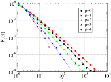
Figure 2: Distribution $P_{p}(\tau)$ of times during which an agent does not change connectivity $p$. $N=10000$, $b_{0}=b_{1}=0.7$, $\lambda=0.8$, and the simulation is run for $T=10^{5}N$ time steps. The lines are the analytical predictions.

In Fig. 3, we also show the distribution of contact durations between two agents (which is different from $P_{1}$: two agents remain in contact when they are joined by a third, but leave the state $p=1$), of triangle durations, and of the time intervals between the starting times of two successive contacts Sociopatterns . This last quantity is highly relevant in the context of causal processes, as it gives the time scale on which an agent can propagate an information or a disease after receiving it. All these distributions are broad, similarly to empirical observations Scherrer:2008 ; Sociopatterns .

Let us finally mention that, when considering parameter values outside the validity of the stationary state analytical computations, different scenarios are observed, depending on $\lambda$: if $\lambda>0.5$, the average state slowly decreases (towards $0$ if $b_{0}<0.5$, and $1$ if $b_{1}<0.5$) while, for $\lambda<0.5$, a large cluster appears, with size is proportional to $N$, and lasting on a diverging timescale. Interestingly, even in this non-stationary case, the shape of the distributions $P_{p}(\tau)$ may remain stationary (not shown). This is particularly relevant as most empirical data are necessarily obtained in non-stationary environments.

In this Letter, we have proposed a modeling framework for dynamical networks in the context of interacting social agents. Both broad and narrow distributions can be obtained, corresponding to different social situations. The present framework can be developed in several research directions. First, many variations of the microscopic rules may be thought of and implemented, in order to model more precisely mechanisms of social contacts in various contexts or even of animal behavior. For instance, merging and splitting of groups could be introduced, as well as heterogeneity between agents to take into account different propensities to interact or to create groups. Moreover, it will be interesting to investigate how the properties of the interaction durations shape the resulting aggregated networks on various timescales. Finally, model dynamical contact networks can be used as a support for the simulation of dynamical processes taking place on dynamical networks, such as information spreading in a conference: the spreading process, although taking place on an extremely sparse network which is at any time formed of disconnected groups, may overall concern the whole population of agents, thanks to the dynamics of the agents who move from one group to another. The fact that the various network characteristics (such as the broadness of the distribution of contact durations and inter-contact times) can be controlled by changing the model’s parameters will then make it possible to understand better the effect of these characteristics on the dynamical processes under scrutiny.

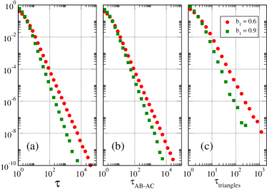
Figure 3: Distributions of (a) duration of a contact between two agents; (b) time intervals between the beginnings of successive contacts of an agent A with two different agents B and C; (c) duration of a triangle. $b_{0}=0.7$, $\lambda=0.8$, $b_{1}=0.6$ and $0.9$. $N=1000$, $T=10^{5}N$.

Acknowledgments This work has been partly supported by the FET Open project DYNANETS (number 233847) funded by the European Commission.

References

- (1) J.-P. Eckmann, E. Moses, D. Sergi, Proc. Natl. Acad. Sci. USA 101 14333 (2004).
- (2) A.-L. Barabási, Nature, 435, 205 (2005).
- (3) D. Rybski et al., Proc. Natl. Acad. Sci. USA 106 12640 (2009).
- (4) J.-P. Onnela et al., Proc. Natl. Acad. Sci. USA 104, 7332 (2007).
- (5) M. C. González, C. A. Hidalgo, A.-L. Barabási, Nature 453, 779-782 (2008).
- (6) P. Huiet al., Proceedings of the 2005 ACM SIGCOMM workshop on Delay-tolerant networking, 244 - 251 (2005).
- (7) N. Eagle, A. Pentland, Personal and Ubiquitous Computing 10, 255-268 (2006).
- (8) E. O’Neill et al. Lecture Notes in Computer Science 4206, 315 (2006).
- (9) A. Pentland, Honest Signals: how they shape our world (MIT Press, Cambridge MA, 2008).
- (10) A. Vázquez et al. Phys. Rev. E 73, 036127 (2006)
- (11) A. Barrat et al., arxiv:0811.4170
- (12) http://www.sociopatterns.org
- (13) H. Alani et al., 8th International Semantic Web Conference (ISWC2009).
- (14) M. Granovetter, AJS 78, 1360 (1973).
- (15) S. Wasserman, K. Faust, Social Network Analysis: Methods and applications (Cambridge University Press, Cambridge, 1994).
- (16) M. E. J. Newman, Proc. Natl. Acad. Sci. (USA) 98, 404 (2001).
- (17) S.N. Dorogovtsev, J.F.F. Mendes, Evolution of networks: From biological nets to the Internet and WWW. (Oxford University Press, Oxford, 2003). M. E. J. Newman, SIAM Review 45, 167 (2003). R. Pastor-Satorras, A. Vespignani, Evolution and structure of the Internet: A statistical physics approach, Cambridge University Press, Cambridge (2004). G. Caldarelli, Scale-Free Networks (Oxford University Press, Oxford, 2007).
- (18) A. Barrat, M. Barthélemy, A. Vespignani, Dynamical processes on complex networks, Cambridge University Press, Cambridge (2008).
- (19) J. M. Kumpula et al. Phys. Rev. Lett. 99, 228701 (2007).
- (20) N.F. Johnson et al., Phys. Rev. E 79, 066117 (2009).
- (21) J. Davidsen, H. Ebel and S. Bornholdt, Phys. Rev. Lett. 88, 128701 (2002).
- (22) M. Marsili et al., Proc. Natl. Acad. Scie. USA 101, 1439 (2004).
- (23) P. Holme and M. E. J. Newman, Phys. Rev. E 74, 056108 (2006).
- (24) F. Vazquez, V. M. Eguíluz and Maxi San Miguel, Phys. Rev. Lett. 100, 108702 (2008).
- (25) A. Scherrer et al., Comp. Net. 52, 2842 (2008).
- (26) A. Vázquez, B. Rácz, A. Lukacs, A.-L. Barabàsi, Phys. Rev. Lett. 98, 158702 (2007).
- (27) P. Holme, Phys. Rev. E 71, 046119 (2005).
- (28) R. Parshani et al., preprint:arXiv:0901.4563
- (29) Adaptive Networks: Theory, Models and Applications, Springer/NECSI Studies on Complexity Series, Gross, T. and Sayama, H. Eds, 2008.
- (30) J. Tang et al., preprint:. arXiv:0909.1712
- (31) A. Gautreau, A. Barrat, M. Barthélemy, Proc. Natl. Acad. Sci. USA 106 8847 (2009).
- (32) S.A. Hill and D. Braha, arxiv:0901.4407
- (33) A.-L. Barabási and R. Albert, Science 286, 509 (1999).
- (34) B. T. J. Morgan, Adv. Appl. Prob. 8, 30 (1976).
- (35) S. Gueron and S. A. Levin, Math. Biosciences 128, 243 (1995).