Abstract

The problem of errors, arising due to finite BPM resolution, in the difference orbit parameters, which are found as a least squares fit to the BPM data, is one of the standard and important problems of accelerator physics. Even so for the case of transversely uncoupled motion the covariance matrix of reconstruction errors can be calculated “by hand”, the direct usage of obtained solution, as a tool for designing of a “good measurement system”, does not look to be fairly straightforward. It seems that a better understanding of the nature of the problem is still desirable. We make a step in this direction introducing dynamic into this problem, which at the first glance seems to be static. We consider a virtual beam consisting of virtual particles obtained as a result of application of reconstruction procedure to “all possible values” of BPM reading errors. This beam propagates along the beam line according to the same rules as any real beam and has all beam dynamical characteristics, such as emittances, energy spread, dispersions, betatron functions and etc. All these values become the properties of the BPM measurement system. One can compare two BPM systems comparing their error emittances and rms error energy spreads, or, for a given measurement system, one can achieve needed balance between coordinate and momentum reconstruction errors by matching the error betatron functions in the point of interest to the desired values.

1 Introduction

The determination of variations in the transverse beam position and in the beam energy using readings of beam position monitors (BPMs) is one of the standard and important problems of accelerator physics. If the optical model of the beam line and BPM resolutions are known, the typical choice is to let jitter parameters be a solution of the weighted linear least squares problem. Even so for the case of transversely uncoupled motion this least squares problem can be solved “by hand”, the direct usage of obtained analytical solution as a tool for designing of a “good measurement system” does not look to be fairly straightforward. It seems that a better understanding of the nature of the problem is still desirable.

A step in this direction was made in the paper [1], where dynamic was introduced into this problem which in the beginning seemed to be static. When one changes the position of the reconstruction point, the estimate of the jitter parameters propagates along the beam line exactly as a particle trajectory and it becomes possible (for every fixed jitter values) to consider a virtual beam consisting from virtual particles obtained as a result of application of least squares reconstruction procedure to “all possible values” of BPM reading errors. The dynamics of the centroid of this beam coincides with the dynamics of the true difference orbit and the covariance matrix of the jitter reconstruction errors can be treated as the matrix of the second central moments of this virtual beam distribution.

In accelerator physics a beam is characterized by its emittances, energy spread, dispersions, betatron functions and etc. All these values immediately become the properties of our BPM measurement system. From now one can compare two BPM systems comparing their error emittances and error energy spreads, or, for a given measurement system, one can achieve needed balance between coordinate and momentum reconstruction errors by matching the error betatron functions in the point of interest to the desired values.

This dynamical point of view on the BPM measurement system was explored in [1] in application to the case of transversely uncoupled nondispersive beam motion and in this paper we continue this study adding energy degree of freedom. The paper by itself is organized as follows. In section 2 we introduce all needed notations, formulate the problem and give its standard least squares solution. As a new element, we formulate the necessary and sufficient conditions for the BPM system to be able to distinguish between transverse and energy jitters in terms of its three BPM subsystems. In section 3 (the core section of this paper) we make parametrization of the covariance matrix of the jitter reconstruction errors using the usual accelerator physics concepts of emittance, energy spread, dispersion and betatron functions. We also show that the error dispersion is not simply one of the many dispersions which could propagate through our beam line. It, in analogy with the error betatron functions [1], is by itself solution of some minimization problem and is uniquely determined by transport matrices between BPM locations and by BPM resolutions. In section 4 we consider the measurement system which utilizes three beam position monitors (the minimum number of BPMs needed) and analyze in details effect of symmetries of the optics between BPM locations. In section 5 we continue the investigation of periodic measurement systems started in [1]. This time with the main accent on achievable energy resolution. And, finally, in section 6 we discuss application of the Courant-Snyder quadratic form as error estimator, even so in the case when energy degree of freedom is taken into account this quadratic form is not bound to be an invariant.

2 Problem and Its Least Squares Solution

Let us consider a magnetostatic beam line which is built from optical elements which are symmetric about the horizontal midplane $\,y=0$. In such magnetic system the transverse particle motion is uncoupled in linear approximation, the vertical oscillations are dispersion free and errors in reconstruction of their parameters were already studied in [1], and in this paper we will examine together $x$-plane and energy degrees of freedom because they are connected through (linear) dispersion.

We will use the variables $\;\vec{z}=(x,\,p,\,\varepsilon)^{\top}\;$ for the description of the horizontal dispersive beam motion. Here, as usual, $\,x\,$ is the horizontal particle coordinate, $\,p\,$ is the horizontal canonical momentum scaled with the kinetic momentum of the reference particle and the variable $\,\varepsilon\,$ stays for the relative energy (or momentum) deviation. As orbit parameters we will understand values of $\,x,\,p\,$ and $\,\varepsilon\,$ given in some predefined point in the beam line (reconstruction point with longitudinal position $\,s=r\,$) and as transverse and energy jitter in this point we will mean the difference

$$\delta\vec{z}(r)\,=\,\left(\,\delta x(r),\,\delta p(r),\,\delta\varepsilon(r)\,\right)^{\top}=\,\left(\,x(r)\,-\,\bar{x}(r),\;p(r)\,-\,\bar{p}(r),\;\varepsilon\,-\,\bar{\varepsilon}\,\right)^{\top}$$ (1)

between parameters of the instantaneous orbit and parameters of some predetermined reference (golden) trajectory $\;(\bar{x},\,\bar{p},\,\bar{\varepsilon})^{\top}$.

Let us assume that we have $n$ BPMs in our beam line placed at positions $\,s_{1},\ldots,s_{n}\,$ and they deliver readings

$$\vec{b}_{c}\;=\;\left(\,b_{1}^{c},\,\ldots\,b_{n}^{c}\,\right)^{\top}$$ (2)

for the current trajectory with previously recorded observations for the golden orbit being

$$\vec{b}_{g}\;=\;\left(\,b_{1}^{g},\,\ldots\,b_{n}^{g}\,\right)^{\top}\,.$$ (3)

Suppose that the difference between these readings can be represented in the form

$$\delta\vec{b}_{\varsigma}\;\stackrel{{\scriptstyle\rm def}}{{=}}\;\vec{b}_{c}\,-\,\vec{b}_{g}\;=\;\left(\begin{array}[]{c}x(s_{1})-\bar{x}(s_{1})\\ \vdots\\ x(s_{n})-\bar{x}(s_{n})\end{array}\right)\;+\;\vec{\,\varsigma}\,,$$ (7)

where the random vector $\,\vec{\,\varsigma}\,=\,(\,\varsigma_{1},\,\ldots,\,\varsigma_{n}\,)^{\top}\,$ has zero mean and positive definite covariance matrix $\,V_{\varsigma}\,$, i.e. that

$$\big{<}\,\vec{\,\varsigma}\,\big{>}\;=\;\vec{\,0},\hskip 19.91684pt{\cal V}\left(\,\vec{\,\varsigma}\,\right)\;=\;\big{<}\,\vec{\,\varsigma}\cdot\vec{\,\varsigma}^{\top}\big{>}\,-\,\big{<}\,\vec{\,\varsigma}\,\big{>}\cdot\big{<}\,\vec{\,\varsigma}\,\big{>}^{\top}\;=\;V_{\varsigma}\;>\;0.$$ (8)

The purpose of this paper is to study the influence of BPM reading errors $\,\vec{\,\varsigma}\,$ on precision of reconstruction of jitter parameters under assumption that optical model of the beam line is known. The additional assumptions which we will make are: the covariance matrix $\,V_{\varsigma}\,$ stays constant and the BPM reading errors can be treated as independent from one measurement to the other. So BPM errors that are correlated from measurement to measurement (calibration and other systematic errors, drifting BPM readings and etc.) and fluctuations in BPM resolutions will be not considered. In practical applications these assumptions may or may not be realistic, but, first, they make the underlying mathematics almost trivial and, second, their satisfaction is, in some sense, one of the goals for the BPM and BPM electronics designers.

Let $\,A_{m}(r)\,$ be a transfer matrix from location of the reconstruction point to the $m$-th BPM location

$$A_{m}(r)\,=\,\left(\begin{array}[]{lll}a_{m}(r)&c_{m}(r)&g_{m}(r)\\ e_{m}(r)&d_{m}(r)&f_{m}(r)\\ 0&0&1\end{array}\right),\hskip 14.22636pta_{m}(r)\,d_{m}(r)-c_{m}(r)\,e_{m}(r)\,\equiv\,1,$$ (12)

and let us assume that the Cholesky factorization $\,V_{\varsigma}=R_{\varsigma}^{\top}R_{\varsigma}\,$ of the covariance matrix $\,V_{\varsigma}\,$ is known. As usual, we will find an estimate

$$\delta\vec{z}_{\varsigma}(r)\;=\;(\delta x_{\varsigma}(r),\,\delta p_{\varsigma}(r),\,\delta\varepsilon_{\varsigma}(r))^{\top}$$ (13)

for the difference orbit parameters (1) in the presence of BPM reading errors by solving the following weighted linear least squares problem

$$\min_{\delta\vec{z}_{\varsigma}}\;\;\left\|M_{\varsigma}\cdot\delta\vec{z}_{\varsigma}\;-\;R_{\varsigma}^{-\top}\cdot\delta\vec{b}_{\varsigma}\,\right\|_{2}^{2}.$$ (14)

Here $\,\|\cdot\|_{2}\,$ denotes the Euclidean vector norm, $\,M_{\varsigma}\,=\,R_{\varsigma}^{-\top}M\,$ and

$$M\;=\;\left(\begin{array}[]{ccc}a_{1}(r)&c_{1}(r)&g_{1}(r)\\ \vdots&\vdots&\vdots\\ a_{n}(r)&c_{n}(r)&g_{n}(r)\end{array}\right).$$ (18)

The problem (14) always has at least one solution and, if we will assume that the matrix $\,M_{\varsigma}\,$ has full column rank $(\mbox{rank}(M_{\varsigma})=3)$, then the solution of this problem is unique and is given by the well known formula

$$\delta\vec{z}_{\varsigma}(r)\;=\;\left(M_{\varsigma}^{\top}(r)M_{\varsigma}(r)\right)^{-1}M_{\varsigma}^{\top}(r)\,R_{\varsigma}^{-\top}\cdot\delta\vec{\,b}_{\varsigma},\;=$$

$$=\;\left(M^{\top}(r)V_{\varsigma}^{-1}M(r)\right)^{-1}M^{\top}(r)\,V_{\varsigma}^{-1}\cdot\delta\vec{\,b}_{\varsigma}\,.$$ (19)

The calculation of the covariance matrix of the errors of this estimate (object of our main interest) is also standard and gives the following result

$$V_{z}(r)\;\stackrel{{\scriptstyle\rm def}}{{=}}\;{\cal V}\left(\,\delta\vec{z}_{\varsigma}(r)\,\right)\;=\;\left(M_{\varsigma}^{\top}(r)M_{\varsigma}(r)\right)^{-1}\;=\;\left(M^{\top}(r)\,V_{\varsigma}^{-1}\,M(r)\right)^{-1}\,.$$ (20)

Let us discuss in more details the important condition for the matrix $\,M_{\varsigma}\,$ to have full column rank. This condition will allow us to separate betatron and dispersion oscillations at the BPM locations and, therefore, will make our system applicable for measuring transverse and energy jitter.

Because the matrix $\,R_{\varsigma}\,$ is nondegenerated, the rank of the matrix $\,M_{\varsigma}\,$ is always equal to the rank of the matrix $\,M$, and the matrix $\,M$, in the next turn, will have full column rank if and only if the Gram determinant $\,\Gamma\left(\vec{a},\,\vec{c},\,\vec{g}\right)\,$ of its column vectors

$$\vec{a}\;=\;\left(a_{1},\ldots,a_{n}\right)^{\top},\hskip 9.95863pt\vec{c}\;=\;\left(c_{1},\ldots,c_{n}\right)^{\top},\hskip 9.95863pt\vec{g}\;=\;\left(g_{1},\ldots,g_{n}\right)^{\top}$$ (21)

is not equal to zero.

To find desired expression for the Gram determinant let us introduce $\,B_{mk}\,$ - transport matrix from the location of the BPM with index $m$ to the location of the BPM with index $k$

$$B_{mk}\;=\;A_{k}\,A_{m}^{-1}\;=\;\left(\begin{array}[]{ccc}\mbox{\ae}_{11}^{mk}&\mbox{\ae}_{12}^{mk}&\mbox{\ae}_{16}^{mk}\\ \mbox{\ae}_{21}^{mk}&\mbox{\ae}_{22}^{mk}&\mbox{\ae}_{26}^{mk}\\ 0&0&1\end{array}\right).$$ (25)

With these notations and using Binet-Cauchy formula one can obtain after some straightforward manipulations

$$\Gamma\left(\vec{a},\,\vec{c},\,\vec{g}\right)\;=\;\det\left(M^{\top}M\right)\;=\;\sum\limits_{1\leq i<j<k\leq n}\left(\mbox{\ae}_{52}^{ij}\,\mbox{\ae}_{12}^{jk}\;-\;\mbox{\ae}_{12}^{ij}\,\mbox{\ae}_{16}^{jk}\right)^{2}\;=$$

$$=\;\frac{1}{6}\sum\limits_{i,\,j,\,k=1}^{n}\left(\mbox{\ae}_{52}^{ij}\,\mbox{\ae}_{12}^{jk}\;-\;\mbox{\ae}_{12}^{ij}\,\mbox{\ae}_{16}^{jk}\right)^{2}\;=\;\frac{1}{6}\sum\limits_{i,\,j,\,k=1}^{n}\left(\mbox{\ae}_{12}^{ij}\,\mbox{\ae}_{16}^{ik}\;-\;\mbox{\ae}_{16}^{ij}\,\mbox{\ae}_{12}^{ik}\right)^{2},$$ (26)

where $\,\mbox{\ae}_{52}^{ij}\,$ (in the framework of the usual 6 by 6 matrix formalism for the linear beam dynamics) is the coefficient that connects variation of the particle path length with variation of the particle transverse momentum and which can be expressed using elements of the matrix $\,B_{ij}\,$ as follows

$$\mbox{\ae}_{52}^{ij}\;=\;\mbox{\ae}_{22}^{ij}\,\mbox{\ae}_{16}^{ij}\;-\;\mbox{\ae}_{12}^{ij}\,\mbox{\ae}_{26}^{ij}\,.$$ (27)

From (26) one sees, that the matrix $\,M\,$ will have the full column rank if and only if there are at least three beam position monitors with indices $\,i,\,j\,$ and $\,k\,$ such that the transport matrices between them satisfy the condition

$$\mbox{\ae}_{52}^{ij}\,\mbox{\ae}_{12}^{jk}\;-\;\mbox{\ae}_{12}^{ij}\,\mbox{\ae}_{16}^{jk}\;\neq\;0$$ (28)

or (equivalently) the condition

$$\mbox{\ae}_{12}^{ij}\,\mbox{\ae}_{16}^{ik}\;-\;\mbox{\ae}_{16}^{ij}\,\mbox{\ae}_{12}^{ik}\;\neq\;0.$$ (29)

Note that both conditions, (28) and (29), involve elements of two transfer matrices, but while (28) uses matrices between neighboring BPMs ($B_{ij}\,$ and $\,B_{jk}$), condition (29) operates with the transport matrices from first to two remaining BPMs ($B_{ij}\,$ and $\,B_{ik}$). In simple words the condition (29), for example, means that one can not vary particle transverse momentum and particle energy at the first BPM location in such a fashion that these variations are invisible at the two downstream BPMs.

3 Beam Dynamical Parametrization of
Covariance Matrix of Reconstruction Errors

Let $\,A(r_{1},\,r_{2})\,$ be a matrix which transport particle coordinates from the point with the longitudinal position $\,s=r_{1}\,$ to the point with the longitudinal position $\,s=r_{2}\,$

$$A(r_{1},\,r_{2})\,=\,\left(\begin{array}[]{lll}m_{11}&m_{12}&m_{16}\\ m_{21}&m_{22}&m_{26}\\ 0&0&1\end{array}\right),\hskip 14.22636ptm_{11}\,m_{22}-m_{12}\,m_{21}\,=\,1.$$ (33)

Similar to [1], one can easily show that for any given value of $\,\vec{\,\varsigma}\,$ the estimate of the difference orbit parameters $\,\delta\vec{z}_{\varsigma}\,$ propagates along the beam line exactly as particle trajectory

$$\delta\vec{z}_{\varsigma}(r_{2})\;=\;A(r_{1},\,r_{2})\cdot\delta\vec{z}_{\varsigma}(r_{1}),$$ (34)

as one changes the position of the reconstruction point. So again we can consider a virtual beam consisting from virtual particles obtained as a result of application of formula (19) to “all possible values” of the error vector $\,\vec{\,\varsigma}$. The dynamics of the centroid of this beam $\,\delta\vec{z}_{0}\,$ coincides with the dynamics of the true difference orbit

$$\delta\vec{z}_{0}(r)\;\stackrel{{\scriptstyle\rm def}}{{=}}\;\big{<}\delta\vec{z}_{\varsigma}(r)\big{>}\;=\;\delta\vec{z}(r)\,,$$ (35)

and the error covariance matrix (20) can be treated as the matrix of the second central moments of this virtual beam distribution and satisfies the usual transport equation

$$V_{z}(r_{2})\;=\;A(r_{1},\,r_{2})\,V_{z}(r_{1})\,A^{\top}(r_{1},\,r_{2}).$$ (36)

Consequently, for the description of the propagation of the reconstruction errors along the beam line, one can use the accelerator physics notations and represent the error covariance matrix in the familiar form

$$V_{z}=\left(M_{\varsigma}^{\top}M_{\varsigma}\right)^{-1}=\epsilon_{\varsigma}\,\left(\begin{array}[]{rrr}\beta_{\varsigma}&-\alpha_{\varsigma}&0\\ -\alpha_{\varsigma}&\gamma_{\varsigma}&0\\ 0&0&0\end{array}\right)+\Delta_{\varsigma}^{2}\,\left(\begin{array}[]{c}\eta_{x,\varsigma}\\ \eta_{p,\varsigma}\\ 1\end{array}\right)\left(\begin{array}[]{c}\eta_{x,\varsigma}\\ \eta_{p,\varsigma}\\ 1\end{array}\right)^{\top}\;=$$ (46)

$$=\;\left(\begin{array}[]{ccc}\epsilon_{\varsigma}\,\beta_{\varsigma}+\Delta_{\varsigma}^{2}\,\eta_{x,\varsigma}^{2}&-\epsilon_{\varsigma}\,\alpha_{\varsigma}+\Delta_{\varsigma}^{2}\,\eta_{x,\varsigma}\,\eta_{p,\varsigma}&\Delta_{\varsigma}^{2}\,\eta_{x,\varsigma}\\ -\epsilon_{\varsigma}\,\alpha_{\varsigma}+\Delta_{\varsigma}^{2}\,\eta_{x,\varsigma}\,\eta_{p,\varsigma}&\epsilon_{\varsigma}\,\gamma_{\varsigma}+\Delta_{\varsigma}^{2}\,\eta_{p,\varsigma}^{2}&\Delta_{\varsigma}^{2}\,\eta_{p,\varsigma}\\ \Delta_{\varsigma}^{2}\,\eta_{x,\varsigma}&\Delta_{\varsigma}^{2}\,\eta_{p,\varsigma}&\Delta_{\varsigma}^{2}\end{array}\right).$$ (50)

As usual for the particle dynamics, this parametrization has two invariants (quantities which are independent from the position of the reconstruction point), namely transverse error emittance $\,\epsilon_{\varsigma}\,$ and rms error energy spread $\,\Delta_{\varsigma}$, which can be calculated according to the formulas

$$\epsilon_{\varsigma}\;=\;\frac{1}{\sqrt{\Gamma\left(\vec{a}_{\varsigma},\,\vec{c}_{\varsigma}\right)}},\hskip 28.45274pt\Delta_{\varsigma}\;=\;\sqrt{\frac{\Gamma\left(\vec{a}_{\varsigma},\,\vec{c}_{\varsigma}\right)}{\Gamma\left(\vec{a}_{\varsigma},\,\vec{c}_{\varsigma},\,\vec{g}_{\varsigma}\right)}},$$ (51)

where we have used the notations

$$\vec{a}_{\varsigma}\;=\;R_{\varsigma}^{-\top}\vec{a},\hskip 19.91684pt\vec{c}_{\varsigma}\;=\;R_{\varsigma}^{-\top}\vec{c},\hskip 19.91684pt\vec{g}_{\varsigma}\;=\;R_{\varsigma}^{-\top}\vec{g}$$ (52)

and $\,\Gamma\left(\vec{u}_{1},\,\ldots\,\vec{u}_{m}\right)\,$ is the Gram determinant of the vectors $\,\vec{u}_{1},\,\ldots\,\vec{u}_{m}$.

The error Twiss parameters, of course, remain the same as they were earlier published in [1], namely

$$\beta_{\varsigma}(r)=\epsilon_{\varsigma}\,\left\|\vec{c}_{\varsigma}(r)\right\|_{2}^{2},\hskip 9.95863pt\alpha_{\varsigma}(r)=\epsilon_{\varsigma}\,\left(\vec{a}_{\varsigma}(r)\cdot\vec{c}_{\varsigma}(r)\right),\hskip 9.95863pt\gamma_{\varsigma}(r)=\epsilon_{\varsigma}\,\left\|\vec{a}_{\varsigma}(r)\right\|_{2}^{2},$$ (53)

and for the new objects, the coordinate and momentum error dispersions, we have

$$\eta_{x,\varsigma}(r)\;=\;\epsilon_{\varsigma}\,\Big{(}\alpha_{\varsigma}(r)\,\left(\vec{c}_{\varsigma}(r)\cdot\vec{g}_{\varsigma}(r)\right)\;-\;\beta_{\varsigma}(r)\,\left(\vec{a}_{\varsigma}(r)\cdot\vec{g}_{\varsigma}(r)\right)\Big{)},$$ (54)

$$\eta_{p,\varsigma}(r)\;=\;\epsilon_{\varsigma}\,\Big{(}\alpha_{\varsigma}(r)\,\left(\vec{a}_{\varsigma}(r)\cdot\vec{g}_{\varsigma}(r)\right)\;-\;\gamma_{\varsigma}(r)\,\left(\vec{c}_{\varsigma}(r)\cdot\vec{g}_{\varsigma}(r)\right)\Big{)}.$$ (55)

As it was shown in [1], the error Twiss parameters (53) are not simply one of many betatron functions which could propagate through our beam line, they are by themselves solutions of some minimization problem and are uniquely determined by transport matrices between BPM locations and by BPM resolutions. And we would like to show, that the same is true also for the error dispersions (54) and (55).

Let $\,\eta_{x}(r)\,$ and $\,\eta_{p}(r)\,$ be some dispersions specified in the reconstruction point. Then the corresponding coordinate dispersion at the $m$-th BPM location can be calculated as follows

$$\eta_{x}(s_{m})\;=\;a_{m}(r)\,\eta_{x}(r)\,+\,c_{m}(r)\,\eta_{p}(r)\,+\,g_{m}(r).$$ (56)

Consider a vector

$$\vec{D}\left(r,\,\eta_{x}(r),\,\eta_{p}(r)\right)=R_{\varsigma}^{-\top}\left(\eta_{x}(s_{1}),\ldots,\eta_{x}(s_{n})\right)^{\top}=\eta_{x}(r)\,\vec{a}_{\varsigma}+\eta_{p}(r)\,\vec{c}_{\varsigma}+\vec{g}_{\varsigma}$$ (57)

and a minimization problem

$$\min_{\eta_{x}(r),\,\eta_{p}(r)}\big{\|}\,\vec{D}\left(r,\,\eta_{x}(r),\,\eta_{p}(r)\right)\,\big{\|}_{2}^{2}.$$ (58)

By standard means it is not difficult to show that if $\,\Gamma\left(\vec{a},\,\vec{c}\right)\neq 0\,$ then the solution of this minimization problem is unique and is given by the formulas (54) and (55).

If, additionally, $\,\Gamma\left(\vec{a},\,\vec{c},\,\vec{g}\right)\neq 0\,$ then the minimum in (58) is bigger than zero (and is equal to zero otherwise) and the following identity holds

$$\big{\|}\,\vec{D}\left(r,\,\eta_{x,\varsigma}(r),\,\eta_{p,\varsigma}(r)\right)\,\big{\|}_{2}^{2}\;=\;\frac{1}{\Delta_{\varsigma}^{2}}\,.$$ (59)

Note that geometrically the vector $\,\eta_{x}(r)\,\vec{a}_{\varsigma}+\eta_{p}(r)\,\vec{c}_{\varsigma}\,$ is nothing else as taken with an opposite sign projection of the vector $\,\vec{g}_{\varsigma}\,$ onto a linear subspace formed by vectors $\,\vec{a}_{\varsigma}\,$ and $\,\vec{c}_{\varsigma}$ and hence the vector $\,\vec{D}\left(r,\,\eta_{x,\varsigma}(r),\,\eta_{p,\varsigma}(r)\right)\,$ is orthogonal to both, vector $\,\vec{a}_{\varsigma}\,$ and vector $\,\vec{c}_{\varsigma}$.

To finish this section let us, for the case when readings of different BPMs are uncorrelated, i.e. when the covariance matrix $\,V_{\varsigma}\,$ is a positive diagonal matrix

$$V_{\varsigma}\;=\;\mbox{diag}\left(\,\sigma_{1}^{2},\,\sigma_{2}^{2},\,\ldots,\,\sigma_{n}^{2}\,\right)\;>\;0\,,$$ (60)

write down the following useful expressions for the Gram determinants

$$\Gamma\left(\vec{a}_{\varsigma},\,\vec{c}_{\varsigma}\right)=\frac{1}{2}\sum\limits_{i,\,j=1}^{n}\left(\frac{\mbox{\ae}_{12}^{ij}}{\sigma_{i}\,\sigma_{j}}\right)^{2},$$ (61)

$$\Gamma\left(\vec{a}_{\varsigma},\vec{c}_{\varsigma},\vec{g}_{\varsigma}\right)=\frac{1}{6}\sum\limits_{i,\,j,\,k=1}^{n}\left(\frac{\mbox{\ae}_{52}^{ij}\mbox{\ae}_{12}^{jk}-\mbox{\ae}_{12}^{ij}\mbox{\ae}_{16}^{jk}}{\sigma_{i}\,\sigma_{j}\,\sigma_{k}}\right)^{2}=\frac{1}{6}\sum\limits_{i,\,j,\,k=1}^{n}\left(\frac{\mbox{\ae}_{12}^{ij}\mbox{\ae}_{16}^{ik}-\mbox{\ae}_{16}^{ij}\mbox{\ae}_{12}^{ik}}{\sigma_{i}\,\sigma_{j}\,\sigma_{k}}\right)^{2},$$ (62)

which enter formulas (51) for the transverse error emittance and for the rms error energy spread.

4 Three BPMs in Symmetric Arrangement

Let us assume that we have three beam position monitors in our beam line which deliver uncorrelated readings with rms resolutions $\sigma_{1}$, $\sigma_{2}$ and $\sigma_{3}$, and let $\,B_{12}\,$ and $\,B_{23}\,$ be transfer matrices between first and second, and between second and third BPM locations respectively

$$B_{12}\;=\;\left(\begin{array}[]{ccc}r_{11}&r_{12}&r_{16}\\ r_{21}&r_{22}&r_{26}\\ 0&0&1\end{array}\right),\hskip 14.22636ptB_{23}\;=\;\left(\begin{array}[]{ccc}m_{11}&m_{12}&m_{16}\\ m_{21}&m_{22}&m_{26}\\ 0&0&1\end{array}\right).$$ (69)

When the phase advance between the first and the second BPMs or the phase advance between the second and the third BPMs is not multiple of $\,180^{\circ}\,$, i.e. when

$$r_{12}^{2}\,+\,m_{12}^{2}\,\neq\,0,$$ (70)

this system can be used for the measurement of the transverse orbit jitter with the transverse error emittance given by the following expression

$$\epsilon_{\varsigma}\;=\;\frac{\sigma_{1}\,\sigma_{2}\,\sigma_{3}}{\sqrt{\,\sigma_{1}^{2}\,m_{12}^{2}\,+\,\sigma_{2}^{2}\,\left(m_{11}\,r_{12}\,+\,r_{22}\,m_{12}\right)^{2}\,+\,\sigma_{3}^{2}\,r_{12}^{2}\,}}\,.$$ (71)

In order to be able to resolve both, transverse and energy, jitters simultaneously we have to assume, additionally to (70), that

$$m_{12}\,r_{52}\,-\,r_{12}\,m_{16}\,\neq\,0\,,$$ (72)

where the $\,r_{52}\,$ and $\,r_{51}\,$ coefficients can be expressed using elements of the matrix $\,B_{12}\,$ as follows

$$\left\{\begin{array}[]{ccc}r_{51}&=&r_{21}r_{16}-r_{11}r_{26}\\ r_{52}&=&r_{22}r_{16}-r_{12}r_{26}\end{array}\right..$$ (75)

With (70) and (72) satisfied, we obtain for the square of the rms error energy spread

$$\Delta^{2}_{\varsigma}\;=\;\frac{\,\sigma_{1}^{2}\,m_{12}^{2}\,+\,\sigma_{2}^{2}\,\left(m_{11}\,r_{12}\,+\,r_{22}\,m_{12}\right)^{2}\,+\,\sigma_{3}^{2}\,r_{12}^{2}\,}{\left(m_{12}\,r_{52}\,-\,r_{12}\,m_{16}\right)^{2}}\,.$$ (76)

To complete description of the covariance matrix of the reconstruction errors (50) for the three BPM case, we also need formulas for the error coordinate and momentum dispersions, and for the error betatron functions. And although it is not very difficult to provide some formulas using (53), (54) and (55), the results are not very informative and it is not easy to derive some nontrivial conclusions from them. So in this section we will give more digestible expressions for error dispersions and error betatron functions making an additional simplifying assumption about our measurement system that the transfer matrix $\,B_{23}\,$ between the second and the third BPM is not an arbitrary beam transport matrix, but is obtained as a result of some symmetry manipulation with the transfer matrix between the first and the second BPM.

4.1 Mirror Symmetric Optical System

Let a magnet system between the second and the third BPMs be a mirror symmetric image of the magnet structure between the first and the second BPM locations. Then

$$B_{23}\;=\;\left(\begin{array}[]{ccc}r_{22}&r_{12}&-r_{52}\\ r_{21}&r_{11}&-r_{51}\\ 0&0&1\end{array}\right).$$ (80)

The transverse error emittance of this measurement system is given by

$$\epsilon_{\varsigma}\;=\;\frac{1}{\left|r_{12}\right|}\cdot\frac{\sigma_{1}\,\sigma_{2}\,\sigma_{3}}{\sqrt{\sigma_{1}^{2}\,+\,4\,\sigma_{2}^{2}\,r_{22}^{2}\,+\,\sigma_{3}^{2}}}\,,$$ (81)

and the error betatron functions at the BPM locations can be calculated as follows

$$\beta_{\varsigma}(s_{1})\;=\;\left|r_{12}\right|\cdot\frac{\sigma_{1}}{\sigma_{2}\,\sigma_{3}}\cdot\frac{4\,\sigma_{2}^{2}\,r_{22}^{2}\,+\,\sigma_{3}^{2}}{\sqrt{\sigma_{1}^{2}\,+\,4\,\sigma_{2}^{2}\,r_{22}^{2}\,+\,\sigma_{3}^{2}}},$$ (82)

$$\alpha_{\varsigma}(s_{1})\;=\;\mbox{sign}\left(r_{12}\right)\cdot\frac{\sigma_{1}}{\sigma_{2}\,\sigma_{3}}\cdot\frac{\,2\,\sigma_{2}^{2}\,r_{22}\,\left(1\,+\,2r_{12}r_{21}\right)\,+\,\sigma_{3}^{2}\,r_{11}\,}{\sqrt{\sigma_{1}^{2}\,+\,4\,\sigma_{2}^{2}\,r_{22}^{2}\,+\,\sigma_{3}^{2}}},$$ (83)

$$\beta_{\varsigma}(s_{2})\;=\;\left|r_{12}\right|\cdot\frac{\sigma_{2}}{\sigma_{1}\,\sigma_{3}}\cdot\frac{\,\sigma_{1}^{2}\,+\,\sigma_{3}^{2}\,}{\sqrt{\sigma_{1}^{2}\,+\,4\,\sigma_{2}^{2}\,r_{22}^{2}\,+\,\sigma_{3}^{2}}},$$ (84)

$$\alpha_{\varsigma}(s_{2})\;=\;\mbox{sign}\left(r_{12}\right)\cdot\left(\frac{\sigma_{1}}{\sigma_{3}}-\frac{\sigma_{3}}{\sigma_{1}}\right)\cdot\frac{\,\sigma_{2}\,r_{22}\,}{\sqrt{\sigma_{1}^{2}\,+\,4\,\sigma_{2}^{2}\,r_{22}^{2}\,+\,\sigma_{3}^{2}}},$$ (85)

$$\beta_{\varsigma}(s_{3})\;=\;\left|r_{12}\right|\cdot\frac{\sigma_{3}}{\sigma_{1}\,\sigma_{2}}\cdot\frac{\sigma_{1}^{2}\,+\,4\,\sigma_{2}^{2}\,r_{22}^{2}}{\sqrt{\sigma_{1}^{2}\,+\,4\,\sigma_{2}^{2}\,r_{22}^{2}\,+\,\sigma_{3}^{2}}},$$ (86)

$$\alpha_{\varsigma}(s_{3})\;=\;-\mbox{sign}\left(r_{12}\right)\cdot\frac{\sigma_{3}}{\sigma_{1}\,\sigma_{2}}\cdot\frac{\,\sigma_{1}^{2}\,r_{11}\,+\,2\,\sigma_{2}^{2}\,r_{22}\,\left(1\,+\,2r_{12}r_{21}\right)\,}{\sqrt{\sigma_{1}^{2}\,+\,4\,\sigma_{2}^{2}\,r_{22}^{2}\,+\,\sigma_{3}^{2}}}.$$ (87)

If we will assume that BPM resolutions follow mirror symmetry of the system, which means that $\,\sigma_{1}\,$ is equal to $\,\sigma_{3}$, then, as it could be expected, the error Twiss parameters will satisfy the following symmetry relations

$$\beta_{\varsigma}(s_{3})=\beta_{\varsigma}(s_{1}),\hskip 19.91684pt\alpha_{\varsigma}(s_{3})=-\alpha_{\varsigma}(s_{1}),\hskip 19.91684pt\alpha_{\varsigma}(s_{2})=0.$$ (88)

For the square of the error energy spread we have the following expression

$$\Delta^{2}_{\varsigma}\;=\;\frac{\sigma_{1}^{2}\,+\,4\,\sigma_{2}^{2}\,r_{22}^{2}\,+\,\sigma_{3}^{2}}{4\,r_{52}^{2}}\,,$$ (89)

and the coordinate and momentum error dispersions at the BPM locations are given below

$$\eta_{x,\varsigma}(s_{1})\;=\;-\frac{2\,\sigma_{1}^{2}\,r_{52}}{\sigma_{1}^{2}\,+\,4\,\sigma_{2}^{2}\,r_{22}^{2}\,+\,\sigma_{3}^{2}},$$ (90)

$$\eta_{p,\varsigma}(s_{1})\;=\;\frac{\,\sigma_{1}^{2}\,\left(r_{16}\,+\,2\,r_{12}\,r_{51}\right)\,-\,4\,\sigma_{2}^{2}\,r_{12}\,r_{22}\,r_{26}\,-\,\sigma_{3}^{2}\,r_{16}\,}{r_{12}\cdot\left(\sigma_{1}^{2}\,+\,4\,\sigma_{2}^{2}\,r_{22}^{2}\,+\,\sigma_{3}^{2}\right)},$$ (91)

$$\eta_{x,\varsigma}(s_{2})\;=\;\frac{4\,\sigma_{2}^{2}\,r_{22}\,r_{52}}{\sigma_{1}^{2}\,+\,4\,\sigma_{2}^{2}\,r_{22}^{2}\,+\,\sigma_{3}^{2}},$$ (92)

$$\eta_{p,\varsigma}(s_{2})\;=\;\left(\sigma_{1}^{2}\,-\,\sigma_{3}^{2}\right)\cdot\frac{r_{52}}{r_{12}\cdot\left(\sigma_{1}^{2}\,+\,4\,\sigma_{2}^{2}\,r_{22}^{2}\,+\,\sigma_{3}^{2}\right)},$$ (93)

$$\eta_{x,\varsigma}(s_{3})\;=\;-\frac{2\,\sigma_{3}^{2}\,r_{52}}{\sigma_{1}^{2}\,+\,4\,\sigma_{2}^{2}\,r_{22}^{2}\,+\,\sigma_{3}^{2}},$$ (94)

$$\eta_{p,\varsigma}(s_{3})\;=\;\frac{\,\sigma_{1}^{2}\,r_{16}\,+\,4\,\sigma_{2}^{2}\,r_{12}\,r_{22}\,r_{26}\,-\,\sigma_{3}^{2}\,\left(r_{16}\,+\,2\,r_{12}\,r_{51}\right)\,}{r_{12}\cdot\left(\sigma_{1}^{2}\,+\,4\,\sigma_{2}^{2}\,r_{22}^{2}\,+\,\sigma_{3}^{2}\right)}.$$ (95)

One sees that if BPM resolutions will follow mirror symmetry of the system, they, similar to the error betatron functions, will satisfy

$$\eta_{x,\varsigma}(s_{3})=\eta_{x,\varsigma}(s_{1}),\hskip 19.91684pt\eta_{p,\varsigma}(s_{3})=-\eta_{p,\varsigma}(s_{1}),\hskip 19.91684pt\eta_{p,\varsigma}(s_{2})=0,$$ (96)

independently if $\,r_{26}\,$ is equal to zero or not. One also sees that if mirror symmetric system can be used for energy jitter measurement (i.e. if $\,r_{52}\neq 0\,$), then the error dispersion is nonzero at the system entrance and exit, again independently if $\,r_{26}\,$ is equal to zero or not.

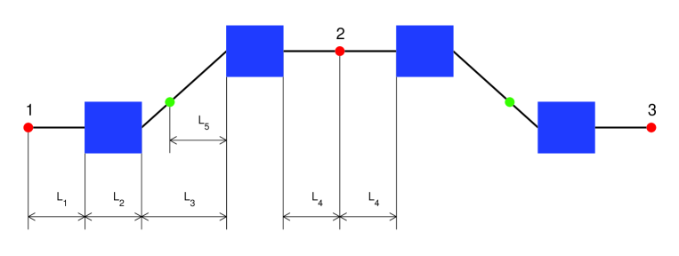
Figure 1: Schematic layout of four bend chicane.

As a more specific example, let us consider three BPMs integrated into four bend magnetic chicane, as shown by red circles in figure 1. For this system

$$B_{12}\;=\;\left(\begin{array}[]{ccc}1&r_{12}&r_{16}\\ 0&1&0\\ 0&0&1\end{array}\right),$$ (100)

where

$$r_{12}\,=\,L_{1}\,+\,L_{4}\,+\,\frac{2\,L_{2}}{\cos(\varphi)}\,+\,\frac{L_{3}}{\cos^{3}(\varphi)}\,\neq\,0$$ (101)

and

$$r_{16}\,=\,r_{52}\,=\,\frac{1}{\cos(\varphi)}\cdot\left(2\,L_{2}\,\tan(\varphi/2)\,+\,\frac{L_{3}}{\cos(\varphi)}\,\tan(\varphi)\right)\,\neq\,0.$$ (102)

Therefore this system always can be used for the transverse and energy jitter measurement, and, as a concrete case, let us consider the first bunch compressor of the FLASH facility [3, 4], which is the four bend chicane of the discussed layout. The typical deflection angle for this chicane is about $18^{\circ}$ and the distances $L_{2}$ and $L_{3}$ are equal each other and are equal to $0.5\,m$ (see, for example, [5]). Let us assume that the first and the third BPMs (orbit BPMs) have the same rms resolutions $\,\sigma_{1}=\sigma_{3}=\sigma_{orb}\,$ and for the second BPM (energy BPM) let us introduce the notation $\,\sigma_{2}=\sigma_{enr}$. Let $\,\Delta_{des}\,$ will be energy jitter resolution desired for the system. With these numbers and notations, and using the usual three sigma criterion $\,(3\Delta_{\varsigma}\leq\Delta_{des})\,$ we obtain from (89) the following inequality

$$\sigma_{orb}^{2}\,+\,2\,\sigma_{enr}^{2}\;\leq\;0.02663\cdot\Delta_{des}^{2}\,,$$ (103)

which gives us limitations on the range of the BPM resolutions which can provide the required precision for the energy jitter measurement. Figure 2, for example, shows the area of acceptable BPM resolutions defined by the inequality (103) for $\,\Delta_{des}=5\cdot 10^{-5}$.

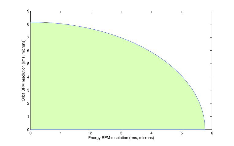
Figure 2: Resolutions of orbit and energy BPMs (shaded area) which are needed in order to be able to resolve energy jitter $5\cdot 10^{-5}$ in the first bunch compressor of the FLASH facility. BPMs are positioned as shown by red circles in figure 1.

To finish the chicane discussion, let us move the first and the third BPMs into positions shown as green circles in figure 1. For this case

$$B_{12}\;=\;\left(\begin{array}[]{ccc}r_{11}&r_{12}&r_{16}\\ 0&r_{22}&r_{26}\\ 0&0&1\end{array}\right),$$ (107)

$$r_{22}\,=\,\frac{1}{r_{11}}\,=\,\cos(\varphi),\hskip 28.45274ptr_{12}\,=\,\frac{L_{5}}{\cos^{2}(\varphi)}\,+\,L_{2}\,+\,L_{4}\,\cos(\varphi),$$ (108)

$$r_{16}\,=\,-L_{2}\,\tan(\varphi/2)\,-\,L_{4}\,\sin(\varphi),\hskip 28.45274ptr_{26}\,=\,-\sin(\varphi),$$ (109)

$$r_{52}\,=\,L_{2}\,\tan(\varphi/2)\,+\,\frac{L_{5}}{\cos(\varphi)}\,\tan(\varphi),$$ (110)

and one sees that this BPM positioning still can be used for the jitter measurement, because $\,r_{12}\neq 0\,$ and $\,r_{52}\neq 0$, but both, the transverse error emittance and the error energy spread become larger (for the same BPM resolutions) than for the original BPM layout. Nevertheless, it is a good example of a mirror symmetric system for which $\,r_{52}\,\neq\,r_{16}\,$ and the total transfer matrix is not achromatic.

4.2 Mirror Antisymmetric Case

If a magnet system between the second and the third BPMs is a mirror antisymmetric image of the first part of the system, then

$$B_{23}\;=\;\left(\begin{array}[]{ccc}r_{22}&r_{12}&r_{52}\\ r_{21}&r_{11}&r_{51}\\ 0&0&1\end{array}\right).$$ (114)

The transverse error emittance and the error beta functions remain the same as for the mirror symmetric case, but the measurement of the energy jitter is not possible anymore, independent of the BPM resolutions following symmetry of the system or not. The coordinate error dispersion is always zero at the BPM locations with the momentum error dispersion taking the values

$$\eta_{p,\varsigma}(s_{1})\,=\,\eta_{p,\varsigma}(s_{3})\,=\,-\frac{r_{16}}{r_{12}},\hskip 28.45274pt\eta_{p,\varsigma}(s_{2})\,=\,-\frac{r_{52}}{r_{12}},$$ (115)

which are independent from BPM resolutions. Note that this impossibility of the energy jitter measurement does not depend on the value of $\,r_{16}\,$ which could be zero or not.

4.3 Two Periodic System

Let us assume that our measurement system is periodic, by which we mean that $\,B_{23}=B_{12}$. We named it in the title as two periodic owing the fact that two equal transfer matrices are involved, but, more correctly, it should be treated as a three cell system because we consider three BPMs. Note that general periodic measurement systems constructed from $n$ identical cells will be studied in details in the next section, but with additional simplifying assumptions that the cell transfer matrix allows periodic beam transport and that all BPMs have the same resolutions.

The transverse error emittance of the two periodic system can be expressed in the form

$$\epsilon_{\varsigma}\;=\;\frac{1}{\left|r_{12}\right|}\cdot\frac{\sigma_{1}\,\sigma_{2}\,\sigma_{3}}{\sqrt{\sigma_{1}^{2}\,+\,\sigma_{2}^{2}\cdot\mbox{tr}_{x}^{2}\left(B_{12}\right)\,+\,\sigma_{3}^{2}}}\,,$$ (116)

where

$$\mbox{tr}_{x}\left(B_{12}\right)\;=\;r_{11}\,+\,r_{22}\,,$$ (117)

and calculation of the error betatron functions gives the following results

$$\beta_{\varsigma}(s_{1})\;=\;\left|r_{12}\right|\cdot\frac{\sigma_{1}}{\sigma_{2}\,\sigma_{3}}\cdot\frac{\sigma_{2}^{2}\cdot\mbox{tr}_{x}^{2}\left(B_{12}\right)\,+\,\sigma_{3}^{2}}{\sqrt{\sigma_{1}^{2}\,+\,\sigma_{2}^{2}\cdot\mbox{tr}_{x}^{2}\left(B_{12}\right)\,+\,\sigma_{3}^{2}}}\,,$$ (118)

$$\alpha_{\varsigma}(s_{1})\;=\;\mbox{sign}\left(r_{12}\right)\cdot\frac{\sigma_{1}}{\sigma_{2}\,\sigma_{3}}\cdot\frac{\sigma_{2}^{2}\cdot\mbox{tr}_{x}\left(B_{12}\right)\cdot\left(r_{11}\cdot\mbox{tr}_{x}\left(B_{12}\right)\,-\,1\right)\,+\,\sigma_{3}^{2}\,r_{11}\,}{\sqrt{\sigma_{1}^{2}\,+\,\sigma_{2}^{2}\cdot\mbox{tr}_{x}^{2}\left(B_{12}\right)\,+\,\sigma_{3}^{2}}}\,,$$ (119)

$$\beta_{\varsigma}(s_{2})\;=\;\left|r_{12}\right|\cdot\frac{\sigma_{2}}{\sigma_{1}\,\sigma_{3}}\cdot\frac{\sigma_{1}^{2}\,+\,\sigma_{3}^{2}}{\sqrt{\sigma_{1}^{2}\,+\,\sigma_{2}^{2}\cdot\mbox{tr}_{x}^{2}\left(B_{12}\right)\,+\,\sigma_{3}^{2}}}\,,$$ (120)

$$\alpha_{\varsigma}(s_{2})\;=\;\mbox{sign}\left(r_{12}\right)\cdot\frac{\sigma_{2}}{\sigma_{1}\,\sigma_{3}}\cdot\frac{\sigma_{1}^{2}\,r_{11}\,-\,\sigma_{3}^{2}\,r_{22}}{\sqrt{\sigma_{1}^{2}\,+\,\sigma_{2}^{2}\cdot\mbox{tr}_{x}^{2}\left(B_{12}\right)\,+\,\sigma_{3}^{2}}}\,,$$ (121)

$$\beta_{\varsigma}(s_{3})\;=\;\left|r_{12}\right|\cdot\frac{\sigma_{3}}{\sigma_{1}\,\sigma_{2}}\cdot\frac{\sigma_{1}^{2}\,+\,\sigma_{2}^{2}\cdot\mbox{tr}_{x}^{2}\left(B_{12}\right)}{\sqrt{\sigma_{1}^{2}\,+\,\sigma_{2}^{2}\cdot\mbox{tr}_{x}^{2}\left(B_{12}\right)\,+\,\sigma_{3}^{2}}}\,,$$ (122)

$$\alpha_{\varsigma}(s_{3})\;=\;-\mbox{sign}\left(r_{12}\right)\cdot\frac{\sigma_{3}}{\sigma_{1}\,\sigma_{2}}\cdot\frac{\,\sigma_{1}^{2}\,r_{22}\,+\,\sigma_{2}^{2}\cdot\mbox{tr}_{x}\left(B_{12}\right)\cdot\left(r_{22}\cdot\mbox{tr}_{x}\left(B_{12}\right)\,-\,1\right)}{\sqrt{\sigma_{1}^{2}\,+\,\sigma_{2}^{2}\cdot\mbox{tr}_{x}^{2}\left(B_{12}\right)\,+\,\sigma_{3}^{2}}}\,.$$ (123)

Let us assume in the following that BPM resolutions follow symmetry of the system, which, in the periodic case, naturally mean that $\,\sigma_{1}=\sigma_{2}=\sigma_{3}$. In this situation $\,\beta_{\varsigma}(s_{1})\,$ and $\,\beta_{\varsigma}(s_{3})\,$ are always equal to each other and, it seems, it is the only symmetry which does not require additional assumptions about coefficients of the cell transport matrix $\,B_{12}$.

The error betatron functions will be cell periodic (will stay unchanged after transport through the first half of the system), if and only if

$$\mbox{tr}_{x}^{2}\left(B_{12}\right)\;=\;1\,,$$ (124)

and, if (124) is satisfied, then

$$\cos(\mu_{p})\;=\;\pm\frac{1}{2}$$ (125)

and, therefore,

$$\sin(3\mu_{p})\,=\,\sin(\mu_{p})\cdot\left(4\cos^{2}(\mu_{p})\,-\,1\right)\,=\,0\,,$$ (126)

where $\,\mu_{p}\,$ is the cell phase advance corresponding to the periodic betatron function.

The error betatron functions will be two cell periodic (will stay unchanged after transport through the whole system), if and only if

$$\mbox{tr}_{x}^{3}\left(B_{12}\right)\;=\;\mbox{tr}_{x}\left(B_{12}\right)\,,$$ (127)

which, when compared with (124), gives equation

$$\mbox{tr}_{x}\left(B_{12}\right)\;=\;0\,,$$ (128)

as the condition for the “true two cell periodicity” (two cell periodic, but not one cell periodic). This condition means that the transverse part of the total system matrix $\,B_{12}^{2}\,$ (two by two submatrix located in the left upper corner) is equal to the minus identity matrix for which arbitrary incoming beta and alpha functions will be transported without changes through the system, but the error betatron functions will also bring the sum of the beta function at the BPM locations to the minimal possible value.

To finish the discussion about error betatron functions let us note, that if in the matrix $\,B_{12}$ the first two diagonal coefficients are to equal each other ($\,r_{11}\,=\,r_{22}\,$), then

$$\alpha_{\varsigma}(s_{3})=-\alpha_{\varsigma}(s_{1}),\hskip 28.45274pt\alpha_{\varsigma}(s_{2})=0,$$ (129)

and one may say that in this situation the error betatron function becomes mirror symmetric.

For the error energy spread and the error coordinate and momentum dispersions we have in the case of the two periodic measurement system the following formulas

$$\Delta^{2}_{\varsigma}\;=\;\frac{\sigma_{1}^{2}\,+\,\sigma_{2}^{2}\cdot\mbox{tr}_{x}^{2}\left(B_{12}\right)\,+\,\sigma_{3}^{2}}{\left(r_{16}\,-\,r_{52}\right)^{2}}\,,$$ (130)

$$\eta_{x,\varsigma}(s_{1})\;=\;\frac{\sigma_{1}^{2}\,\left(r_{16}\,-\,r_{52}\right)}{\sigma_{1}^{2}\,+\,\sigma_{2}^{2}\cdot\mbox{tr}_{x}^{2}\left(B_{12}\right)\,+\,\sigma_{3}^{2}}\,,$$ (131)

$$\eta_{p,\varsigma}(s_{1})\;=$$

$$=-\frac{\sigma_{1}^{2}\left(r_{16}+r_{11}\left(r_{16}-r_{52}\right)\right)+\sigma_{2}^{2}\cdot\mbox{tr}_{x}\left(B_{12}\right)\cdot\left(\left(\mbox{tr}_{x}\left(B_{12}\right)+1\right)r_{16}-r_{52}\right)+\sigma_{3}^{2}r_{16}}{r_{12}\cdot\left(\sigma_{1}^{2}\,+\,\sigma_{2}^{2}\cdot\mbox{tr}_{x}^{2}\left(B_{12}\right)\,+\,\sigma_{3}^{2}\right)}\,,$$ (132)

$$\eta_{x,\varsigma}(s_{2})\;=\;-\frac{\sigma_{2}^{2}\cdot\mbox{tr}_{x}\left(B_{12}\right)\cdot\left(r_{16}\,-\,r_{52}\right)}{\sigma_{1}^{2}\,+\,\sigma_{2}^{2}\cdot\mbox{tr}_{x}^{2}\left(B_{12}\right)\,+\,\sigma_{3}^{2}}\,,$$ (133)

$$\eta_{p,\varsigma}(s_{2})\;=$$

$$=-\frac{\sigma_{1}^{2}r_{16}+\sigma_{2}^{2}\cdot\mbox{tr}_{x}\left(B_{12}\right)\cdot\left(\mbox{tr}_{x}\left(B_{12}\right)\cdot r_{52}+r_{22}\left(r_{16}-r_{52}\right)\right)+\sigma_{3}^{2}r_{52}}{r_{12}\cdot\left(\sigma_{1}^{2}\,+\,\sigma_{2}^{2}\cdot\mbox{tr}_{x}^{2}\left(B_{12}\right)\,+\,\sigma_{3}^{2}\right)}\,,$$ (134)

$$\eta_{x,\varsigma}(s_{3})\;=\;\frac{\sigma_{3}^{2}\,\left(r_{16}\,-\,r_{52}\right)}{\sigma_{1}^{2}\,+\,\sigma_{2}^{2}\cdot\mbox{tr}_{x}^{2}\left(B_{12}\right)\,+\,\sigma_{3}^{2}}\,,$$ (135)

$$\eta_{p,\varsigma}(s_{3})\;=$$

$$=-\frac{\sigma_{1}^{2}r_{52}+\sigma_{2}^{2}\cdot\mbox{tr}_{x}\left(B_{12}\right)\cdot\left(\left(\mbox{tr}_{x}\left(B_{12}\right)+1\right)r_{52}-r_{16}\right)+\sigma_{3}^{2}\left(r_{52}+r_{22}\left(r_{52}-r_{16}\right)\right)}{r_{12}\cdot\left(\sigma_{1}^{2}\,+\,\sigma_{2}^{2}\cdot\mbox{tr}_{x}^{2}\left(B_{12}\right)\,+\,\sigma_{3}^{2}\right)}\,,$$ (136)

and, if resolutions of all three BPMs will be equal, the error dispersion will satisfy the equality

$$\eta_{x,\varsigma}(s_{1})\;=\;\eta_{x,\varsigma}(s_{3})\,.$$ (137)

The condition for the error dispersion to be cell periodic is more restrictive than for the error betatron functions, namely

$$\mbox{tr}_{x}\left(B_{12}\right)\;=\;-1\,,$$ (138)

and the condition for the “true two cell periodicity” is

$$\mbox{tr}_{x}\left(B_{12}\right)\;=\;-2\,,$$ (139)

which does not lead to any noticeable symmetry of the error betatron functions and which means that the transverse part of the cell matrix $\,B_{12}\,$ is equal to the sum of the minus identity matrix plus some nilpotent matrix $\,N\,$ ($\,N^{2}=0\,$).

Note that under condition (138) we have for the periodic cell phase advance the following relations

$$\cos(\mu_{p})\,=\,-\frac{1}{2},\hskip 28.45274pt\sin(3\mu_{p}/2)\,=\,\sin(\mu_{p}/2)\cdot\left(2\cos(\mu_{p})\,+\,1\right)\,=\,0.$$ (140)

4.4 Cell Followed by Switched Cell

If a magnet system between the second and the third BPMs repeats the magnet system between the first and the second BPMs but with switched directions of dipole magnets, then

$$B_{23}\;=\;\left(\begin{array}[]{ccc}r_{11}&r_{12}&-r_{16}\\ r_{21}&r_{22}&-r_{26}\\ 0&0&1\end{array}\right).$$ (144)

In analogy with transition from mirror symmetric to mirror antisymmetric case, the transverse error emittance and the error betatron functions remain the same as for the two periodic measurement system, but, in contrast to mirror antisymmetric case, this system still can be used for the energy jitter measurement if

$$r_{16}\,+\,r_{52}\;\neq\;0\,,$$ (145)

which, in particular, forbids the magnet system between the first and the second BPMs to be mirror symmetric by itself.

For this measurement system we obtain

$$\Delta^{2}_{\varsigma}\;=\;\frac{\sigma_{1}^{2}\,+\,\sigma_{2}^{2}\cdot\mbox{tr}_{x}^{2}\left(B_{12}\right)\,+\,\sigma_{3}^{2}}{\left(r_{16}\,+\,r_{52}\right)^{2}}\,,$$ (146)

$$\eta_{x,\varsigma}(s_{1})\;=\;-\frac{\sigma_{1}^{2}\,\left(r_{16}\,+\,r_{52}\right)}{\sigma_{1}^{2}\,+\,\sigma_{2}^{2}\cdot\mbox{tr}_{x}^{2}\left(B_{12}\right)\,+\,\sigma_{3}^{2}}\,,$$ (147)

$$\eta_{p,\varsigma}(s_{1})\;=$$

$$=-\frac{\sigma_{1}^{2}\left(r_{16}-r_{11}\left(r_{16}+r_{52}\right)\right)+\sigma_{2}^{2}\cdot\mbox{tr}_{x}\left(B_{12}\right)\cdot\left(\left(\mbox{tr}_{x}\left(B_{12}\right)-1\right)r_{16}-r_{52}\right)+\sigma_{3}^{2}r_{16}}{r_{12}\cdot\left(\sigma_{1}^{2}\,+\,\sigma_{2}^{2}\cdot\mbox{tr}_{x}^{2}\left(B_{12}\right)\,+\,\sigma_{3}^{2}\right)}\,,$$ (148)

$$\eta_{x,\varsigma}(s_{2})\;=\;\frac{\sigma_{2}^{2}\cdot\mbox{tr}_{x}\left(B_{12}\right)\cdot\left(r_{16}\,+\,r_{52}\right)}{\sigma_{1}^{2}\,+\,\sigma_{2}^{2}\cdot\mbox{tr}_{x}^{2}\left(B_{12}\right)\,+\,\sigma_{3}^{2}}\,,$$ (149)

$$\eta_{p,\varsigma}(s_{2})\;=$$

$$=\frac{\sigma_{1}^{2}r_{16}-\sigma_{2}^{2}\cdot\mbox{tr}_{x}\left(B_{12}\right)\cdot\left(\mbox{tr}_{x}\left(B_{12}\right)\cdot r_{52}-r_{22}\left(r_{16}+r_{52}\right)\right)-\sigma_{3}^{2}r_{52}}{r_{12}\cdot\left(\sigma_{1}^{2}\,+\,\sigma_{2}^{2}\cdot\mbox{tr}_{x}^{2}\left(B_{12}\right)\,+\,\sigma_{3}^{2}\right)}\,,$$ (150)

$$\eta_{x,\varsigma}(s_{3})\;=\;-\frac{\sigma_{3}^{2}\,\left(r_{16}\,+\,r_{52}\right)}{\sigma_{1}^{2}\,+\,\sigma_{2}^{2}\cdot\mbox{tr}_{x}^{2}\left(B_{12}\right)\,+\,\sigma_{3}^{2}}\,,$$ (151)

$$\eta_{p,\varsigma}(s_{3})\;=$$

$$=\frac{\sigma_{1}^{2}r_{52}+\sigma_{2}^{2}\cdot\mbox{tr}_{x}\left(B_{12}\right)\cdot\left(\left(\mbox{tr}_{x}\left(B_{12}\right)-1\right)r_{52}-r_{16}\right)+\sigma_{3}^{2}\left(r_{52}-r_{22}\left(r_{52}+r_{16}\right)\right)}{r_{12}\cdot\left(\sigma_{1}^{2}\,+\,\sigma_{2}^{2}\cdot\mbox{tr}_{x}^{2}\left(B_{12}\right)\,+\,\sigma_{3}^{2}\right)}\,,$$ (152)

and one sees that for equal BPM resolutions the property

$$\eta_{x,\varsigma}(s_{1})\;=\;\eta_{x,\varsigma}(s_{3})$$ (153)

is still preserved.

There is no reasons to expect that coordinate error dispersion and simultaneously momentum error dispersion could stay constant at all three BPM locations (analogy of cell periodicity for the two cell measurement system) and, as one can check, there is no solution for that. Nevertheless, both error dispersions still can stay unchanged after transport through the whole system, if

$$\mbox{tr}_{x}\left(B_{12}\right)\,=\,1\hskip 19.91684pt\mbox{or}\hskip 19.91684pt\mbox{tr}_{x}\left(B_{12}\right)\,=\,2.$$ (154)

5 Periodic Measurement Systems

Let us consider a measurement system constructed from $n$ identical cells assuming that the cell transfer matrix allows periodic beam transport with phase advance per cell $\,\mu_{p}\,$ being not a multiple of $\,180^{\circ}$. Additionally, we will assume that BPMs placed in our beam line deliver uncorrelated readings, all with the same rms resolution $\,\sigma_{bpm}$.

Let us first consider the case when we have one BPM per cell (identically positioned in all cells) with the periodic betatron function and the periodic dispersion function at the BPM locations equal to $\,\beta_{p}(s_{1})\,$ and $\,\eta_{x,p}(s_{1})\neq 0\,$ respectively.

In this situation the formulas for the error transverse emittance and the error betatron function remain the same as was already published in [1], and the square of the error energy spread is given by the following expression

$$\Delta^{2}_{\varsigma}\;=\;\frac{\sigma^{2}_{bpm}}{n\,\eta_{x,p}^{2}(s_{1})}\cdot\varrho_{n}(\mu_{p})\,,$$ (155)

where the function

$$\varrho_{n}(\mu_{p})\;=\;\frac{1\;+\;\dfrac{1}{n}\cdot\dfrac{\sin(n\mu_{p})}{\sin(\mu_{p})}}{\;1\;+\;\dfrac{1}{n}\cdot\dfrac{\sin(n\mu_{p})}{\sin(\mu_{p})}\;-\;2\left(\dfrac{1}{n}\cdot\dfrac{\sin(n\mu_{p}/2)}{\sin(\mu_{p}/2)}\right)^{2}\;}$$ (156)

is defined only for $\,n\geq 3$. Note that for $\,n\geq 3\,$ this function could be extended by continuity for all $\,\mu_{p}\,$ not multiple of $360^{\circ}$ where it becomes unbounded.

The coordinate and momentum error dispersions $\,\eta_{x,\varsigma}\,$ and $\,\eta_{p,\varsigma}\,$ at the BPM locations are given below

$$\eta_{x,\varsigma}(s_{k})\;=\;\eta_{x,p}(s_{1})\cdot\left(1\;-\;\omega_{n}(\mu_{p})\cdot\cos\left(\tfrac{n+1-2k}{2}\,\mu_{p}\right)\right)\,,$$ (157)

$$\eta_{p,\varsigma}(s_{k})\;=\;\eta_{p,p}(s_{1})\;-\;\eta_{x,p}(s_{1})\cdot\frac{\omega_{n}(\mu_{p})}{\beta_{p}(s_{1})}\left(\sin\left(\tfrac{n+1-2k}{2}\,\mu_{p}\right)\;-\right.$$

$$\left.-\;\alpha_{p}(s_{1})\cdot\cos\left(\tfrac{n+1-2k}{2}\,\mu_{p}\right)\right)\,,$$ (158)

$$\omega_{n}(\mu_{p})\;=\;2\,\left(\dfrac{1}{n}\cdot\dfrac{\sin(n\mu_{p}/2)}{\sin(\mu_{p}/2)}\right)\left(1\;+\;\dfrac{1}{n}\cdot\dfrac{\sin(n\mu_{p})}{\sin(\mu_{p})}\right)^{-1}\,,$$ (159)

and one sees that while the coordinate error dispersion $\,\eta_{x,\varsigma}\,$ always have mirror symmetry

$$\eta_{x,\varsigma}(s_{k})\;=\;\eta_{x,\varsigma}(s_{n+1-k})\,,\hskip 28.45274ptk\;=\;1,\,\ldots,\,n,$$ (160)

the momentum error dispersion will be mirror antisymmetric

$$\eta_{p,\varsigma}(s_{k})\;=\;-\eta_{p,\varsigma}(s_{n+1-k})\,,\hskip 28.45274ptk\;=\;1,\,\ldots,\,n$$ (161)

only in the case when $\,\alpha_{p}(s_{1})\,=\,0\,$ and $\,\eta_{p,p}(s_{1})\,=\,0$.

Note, that the mean value of the coordinate error dispersion and the mean value of its squares satisfy the following relations

$$\frac{1}{n}\,\sum_{k=1}^{n}\eta_{x,\varsigma}(s_{k})\;=\;\frac{\eta_{x,p}(s_{1})}{\varrho_{n}(\mu_{p})}\,,\hskip 28.45274pt\frac{1}{n}\,\sum_{k=1}^{n}\eta_{x,\varsigma}^{2}(s_{k})\;=\;\frac{\eta_{x,p}^{2}(s_{1})}{\varrho_{n}(\mu_{p})}\,.$$ (162)

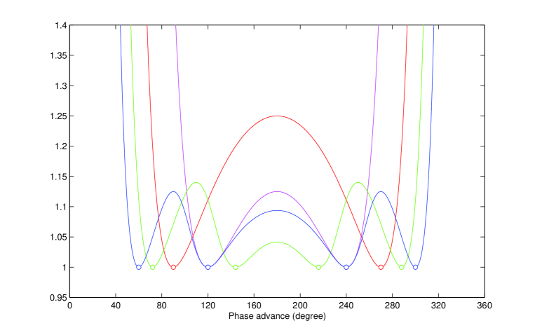
Figure 3: Functions $\,\varrho_{n}(\mu_{p})\,$ shown for $\,n=3,4,5,6\,$ (magenta, red, green and blue curves respectively).

The function $\,\varrho_{n}(\mu_{p})\,$ is never smaller than one and is equal to one (reaches its minimum) only in the points

$$\mu_{p}=k\,\frac{360^{\circ}}{n}\;(\mbox{mod}\;360^{\circ}),\hskip 8.5359ptk=\left\{\begin{array}[]{ll}1,\ldots,n-1&\mbox{\;\,if $\,n\,$ is odd}\\ 1,\ldots,\frac{n}{2}-1,\frac{n}{2}+1,\ldots,n-1&\mbox{\;\,if $\,n\,$ is even}\end{array}\right.$$ (165)

in which error dispersion coincides with periodic dispersion and which seem to be good candidates to be selected for improving resolution of the energy jitter measurement (see figure 3), if we are free in choosing the cell phase advance while, for some reasons, the dispersion at the BPM location has to stay unchanged. But, when we optimize a cell in which periodic dispersion at the BPM location is by itself function of the cell phase advance, the situation, of course, changes. Let us, like in [1], consider a thin lens FODO cell of the length $L$ in which two identical thin lens dipoles with transfer matrix

$$\left(\begin{array}[]{ccc}1&0&0\\ 0&1&\varphi/2\\ 0&0&1\end{array}\right)$$ (169)

are inserted in the middle of drift spaces separating the focusing and defocusing lenses. Let us assume that the BPM is placed in the “center” of the focusing lens with the periodic dispersion at this locations being

$$\eta_{x,p}(s_{1})\;=\;\eta_{+}\;=\;\frac{L\varphi}{4}\cdot\frac{1+\frac{1}{2}\sin(\mu_{p}/2)}{\sin^{2}(\mu_{p}/2)}\,,$$ (170)

where $\,\varphi\,$ is the cell deflection angle.

In this situation we can write

$$\Delta^{2}_{\varsigma}\;=\;\frac{\sigma^{2}_{bpm}}{n}\left(\frac{4}{L\varphi}\right)^{2}\cdot\Psi_{n}(\mu_{p})\,,$$ (171)

where functions $\,\Psi_{n}\,$ depend only on the cell phase advance $\,\mu_{p}\,$ and are converging (from above) to the function

$$\Psi_{\infty}(\mu_{p})\,=\,\frac{\sin^{4}(\mu_{p}/2)}{\left(1+\frac{1}{2}\sin(\mu_{p}/2)\right)^{2}}$$ (172)

as $n$ goes to infinity.

The functions $\,\Psi_{n}\left(\mu_{p}\right)\,$ for $\,n=3,4,5,6\,$ are plotted in figure 4 together with their values in the points (165) shown as small circles at the corresponding curves. One sees that, again like in [1], there is nothing really special about points (165) except the trivial fact that all of them belong to the graph of the function $\,\Psi_{\infty}\,$.

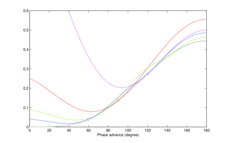
Figure 4: Functions $\,\Psi_{n}(\mu_{p})\,$ shown for $\,n=3,4,5,6\,$ (magenta, red, green and blue curves respectively). The gray curve shows function $\Psi_{\infty}(\mu_{p})$.

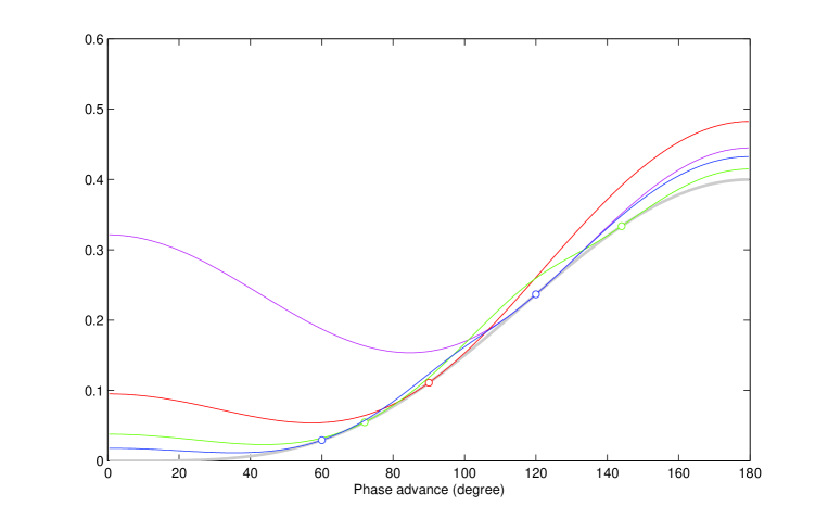
Figure 5: Functions $\,\Phi_{n}(\mu_{p})\,$ shown for $\,n=3,4,5,6\,$ (magenta, red, green and blue curves respectively). The gray curve shows function $\Phi_{\infty}(\mu_{p})$.

Before switching to the situation when we have two BPMs per cell let us rewrite expression (156) for the function $\,\varrho_{n}(\mu_{p})\,$ in the form

$$\varrho_{n}(\mu_{p})\,=\,\left(1\,-\,\frac{\beta_{p}(s_{1})}{2\,m_{p}\left(\beta_{\varsigma},\,\beta_{p}\right)\,\eta_{x,p}^{2}(s_{1})}\cdot I_{x}\left(\beta_{\varsigma},\,\eta_{x,\varsigma}-\eta_{x,p},\,\eta_{p,\varsigma}-\eta_{p,p}\right)\right)^{-1},$$ (173)

where

$$m_{p}\left(\beta_{\varsigma},\,\beta_{p}\right)=\left(1\,-\,\left(\frac{1}{n}\cdot\frac{\sin(n\mu_{p})}{\sin(\mu_{p})}\right)^{2}\right)^{-\frac{1}{2}}$$ (174)

is the mismatch between the error and the periodic betatron functions (even so we do not assume, in general, periodic betatron functions and/or periodic dispersion being the design betatron functions and/or design dispersion matched to our beam line) and

$$I_{x}\left(\beta_{\varsigma},\,\eta_{x,\varsigma}-\eta_{x,p},\,\eta_{p,\varsigma}-\eta_{p,p}\right)\;=$$

$$=\;\gamma_{\varsigma}\left(\eta_{x,\varsigma}-\eta_{x,p}\right)^{2}\,+\,2\alpha_{\varsigma}\left(\eta_{x,\varsigma}-\eta_{x,p}\right)\left(\eta_{p,\varsigma}-\eta_{p,p}\right)\,+\,\beta_{\varsigma}\left(\eta_{p,\varsigma}-\eta_{p,p}\right)^{2}\;=$$

$$=\;\frac{4\,\eta_{x,p}^{2}(s_{1})\,m_{p}^{3}\left(\beta_{\varsigma},\,\beta_{p}\right)}{\beta_{p}(s_{1})}\cdot\left(\frac{1}{n}\cdot\frac{\sin(n\mu_{p}/2)}{\sin(\mu_{p}/2)}\right)^{2}\cdot\left(1\;-\;\frac{1}{n}\cdot\frac{\sin(n\mu_{p})}{\sin(\mu_{p})}\right)$$ (175)

is the difference between periodic and error dispersions measured by using the Courant-Snyder invariant formed out of error Twiss parameters.

Note, for completeness, that if one will express the difference between periodic and error dispersions using Courant-Snyder invariant formed using periodic Twiss parameters, then one will have the following relation

$$I_{x}\left(\beta_{p},\,\eta_{x,\varsigma}-\eta_{x,p},\,\eta_{p,\varsigma}-\eta_{p,p}\right)\;=$$

$$=\;m_{p}\left(\beta_{\varsigma},\,\beta_{p}\right)\left(1\;-\;\frac{1}{n}\cdot\frac{\sin(n\mu_{p})}{\sin(\mu_{p})}\right)\cdot I_{x}\left(\beta_{\varsigma},\,\eta_{x,\varsigma}-\eta_{x,p},\,\eta_{p,\varsigma}-\eta_{p,p}\right)\;=$$

$$=\;\sqrt{\dfrac{1\;-\;\dfrac{1}{n}\cdot\dfrac{\sin(n\mu_{p})}{\sin(\mu_{p})}}{1\;+\;\dfrac{1}{n}\cdot\dfrac{\sin(n\mu_{p})}{\sin(\mu_{p})}}}\cdot I_{x}\left(\beta_{\varsigma},\,\eta_{x,\varsigma}-\eta_{x,p},\,\eta_{p,\varsigma}-\eta_{p,p}\right)\,.$$ (176)

Let us now turn to the situation when we have two BPMs per cell with $\,\theta\,$ being the phase shift between the first and second BPM location.

In this situation the square of the error energy spread can be expressed as

$$\Delta^{2}_{\varsigma}=\frac{\sigma^{2}_{bpm}}{n\left(\eta_{x,p}^{2}(s_{1})+\eta_{x,p}^{2}(s_{2})\right)}\cdot\varpi_{n}\,,$$ (177)

where multiplier

$$\varpi_{n}=\left(1-\frac{\beta_{p}(s_{1})+\beta_{p}(s_{2})}{2m_{p}\left(\beta_{\varsigma},\beta_{p}\right)\left(\eta_{x,p}^{2}(s_{1})+\eta_{x,p}^{2}(s_{2})\right)}\cdot I_{x}\left(\beta_{\varsigma},\eta_{x,\varsigma}-\eta_{x,p},\eta_{p,\varsigma}-\eta_{p,p}\right)\right)^{-1}$$ (178)

has a form which is very similar to (173) with

$$I_{x}\left(\beta_{\varsigma},\,\eta_{x,\varsigma}-\eta_{x,p},\,\eta_{p,\varsigma}-\eta_{p,p}\right)\;=$$

$$=\;\gamma_{\varsigma}\left(\eta_{x,\varsigma}-\eta_{x,p}\right)^{2}\,+\,2\alpha_{\varsigma}\left(\eta_{x,\varsigma}-\eta_{x,p}\right)\left(\eta_{p,\varsigma}-\eta_{p,p}\right)\,+\,\beta_{\varsigma}\left(\eta_{p,\varsigma}-\eta_{p,p}\right)^{2}\;=$$

$$=\frac{4\left(\eta_{x,p}^{2}(s_{1})+\eta_{x,p}^{2}(s_{2})\right)m_{p}^{3}\left(\beta_{\varsigma},\beta_{p}\right)}{\beta_{p}(s_{1})+\beta_{p}(s_{2})}\cdot\left(\frac{1}{n}\cdot\frac{\sin(n\mu_{p}/2)}{\sin(\mu_{p}/2)}\right)^{2}\Bigg{[}\left(1-\frac{1}{n}\cdot\frac{\sin(n\mu_{p})}{\sin(\mu_{p})}\right)\cdot\Bigg{.}$$

$$\cdot\frac{\beta_{p}(s_{1})\,\eta_{x,p}^{2}(s_{1})\,+\,2\cos(\theta)\sqrt{\beta_{p}(s_{1})\,\beta_{p}(s_{2})}\,\eta_{x,p}(s_{1})\,\eta_{x,p}(s_{2})\,+\,\beta_{p}(s_{2})\,\eta_{x,p}^{2}(s_{2})}{\left(\beta_{p}(s_{1})\,+\,\beta_{p}(s_{2})\right)\left(\eta_{x,p}^{2}(s_{1})\,+\,\eta_{x,p}^{2}(s_{2})\right)}\;+$$

$$\Bigg{.}+\;2\sin^{2}(\theta)\frac{\beta_{p}(s_{1})\,\beta_{p}(s_{2})}{\left(\beta_{p}(s_{1})+\beta_{p}(s_{2})\right)^{2}}\cdot\left(\frac{1}{n}\cdot\frac{\sin(n\mu_{p})}{\sin(\mu_{p})}\right)\Bigg{]}$$ (179)

and with the mismatch between the error and the periodic betatron functions having now the following form

$$m_{p}\left(\beta_{\varsigma},\,\beta_{p}\right)=\left(1-\left(1-4\sin^{2}(\theta)\frac{\beta_{p}(s_{1})\beta_{p}(s_{2})}{\left(\beta_{p}(s_{1})+\beta_{p}(s_{2})\right)^{2}}\right)\left(\frac{1}{n}\cdot\frac{\sin(n\mu_{p})}{\sin(\mu_{p})}\right)^{2}\right)^{-\frac{1}{2}}\,.$$ (180)

For a thin lens FODO cell with BPMs placed in the “centers” of focusing and defocusing lenses we have $\,\theta\,=\,\mu_{p}/2\,$ and the periodic beta function and the periodic dispersion at the BPM locations are equal to

$$\beta_{\pm}\;=\;L\cdot\frac{1\,\pm\,\sin(\mu_{p}/2)}{\sin(\mu_{p})}\,,\hskip 14.22636pt\eta_{\pm}\;=\;\frac{L\varphi}{4}\cdot\frac{1\,\pm\,\frac{1}{2}\sin(\mu_{p}/2)}{\sin^{2}(\mu_{p}/2)}\,.$$ (181)

With these assumptions we can write

$$\Delta^{2}_{\varsigma}\;=\;\frac{\sigma^{2}_{bpm}}{n}\left(\frac{4}{L\varphi}\right)^{2}\cdot\Phi_{n}(\mu_{p})\,,$$ (182)

with functions $\Phi_{n}(\mu_{p})$ converging to the function

$$\Phi_{\infty}(\mu_{p})\,=\,\frac{\sin^{4}(\mu_{p}/2)}{2+\frac{1}{2}\sin^{2}(\mu_{p}/2)}$$ (183)

as $n$ goes to infinity.

The functions $\,\Phi_{n}\left(\mu_{p}\right)\,$ for $\,n=3,4,5,6\,$ are plotted in figure 5 and one can see that though we are using two times larger number of BPMs, the energy resolution improves mainly in the region of the low phase advances, while for the high phase advances it stays almost unchanged. To understand the situation better, it is useful to look at the figure 6 where the ratio of the limiting functions $\,\Psi_{\infty}\,$ and $\,\Phi_{\infty}\,$ is shown.

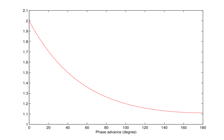
Figure 6: Ratio $\,\Psi_{\infty}\,/\,\Phi_{\infty}$ as a function of the phase advance $\,\mu_{p}$.

6 Courant-Snyder Invariant as Error Estimator

When we consider the jitter problem, the subject of our real interest is the actual difference $\,\delta\vec{z}_{0}\,$ between parameters of the instantaneous and the golden trajectory. Our measurement system delivers us an estimate $\,\delta\vec{z}_{\varsigma}\,$ of this parameter, which includes the effect of the BPM reading errors $\,\vec{\,\varsigma}$.

Thus, in the framework of the model considered, the only information which we could obtain about the true difference $\,\delta\vec{z}_{0}\,$ is the statistical information based on the properties of the random variable $\,\delta\vec{z}_{\varsigma}-\delta\vec{z}_{0}$, which, due to our assumptions, has zero mean and whose statistical distribution does not depend on the actual value of $\,\delta\vec{z}_{0}\,$.

It seems to be natural to use the module $\,\left|\delta\varepsilon_{\varsigma}-\delta\varepsilon_{0}\right|\,$ as a numerical measure of the difference between estimated and true beam energies, but the quantitative measure of the difference $\,\delta\vec{z}_{\varsigma}-\delta\vec{z}_{0}\,$ from zero in the transverse phase space could be chosen differently. One may simply use the Euclidean vector norm, but, as it was already stated in [1], the usage of the Courant-Snyder quadratic form has certain advantages. For example, when one considers errors only in the reconstruction of the transverse orbit parameters in the beam line without dispersion, the Courant-Snyder quadratic form is an invariant and therefore all estimates based on it do not depend on the position of the reconstruction point. And, as one will see below, even for dispersive particle motion the Courant-Snyder quadratic form is a “much better conserved quantity” than the Euclidean norm.

6.1 Transverse Jitter

Let us first return to the situation whose study was already started in paper [1], where we considered errors in the reconstruction of transverse orbit parameters in the beam line without dispersion.

Let $\,\beta_{0}(r),\,\alpha_{0}(r)\,$ and $\,\gamma_{0}(r)\,$ be the design betatron functions, and

$$I_{x}(\,r,\,x,\,p\,)\;=\;\gamma_{0}(r)\,x^{2}\;+\;2\,\alpha_{0}(r)\,x\,p\;+\;\beta_{0}(r)\,p^{2}$$ (184)

be the corresponding Courant-Snyder quadratic form.

According to the above discussion, the object of our current interest is the random variable

$$I_{x}^{\varsigma}\;=\;I_{x}(\,r,\,\,\delta x_{\varsigma}-\delta x_{0}\,,\,\delta p_{\varsigma}-\delta p_{0}\,).$$ (185)

The mean value of this random variable was already calculated in [1] and is equal

$$\big{<}\,I_{x}^{\varsigma}\,\big{>}\;=\;2\,\epsilon_{\varsigma}\,m_{p}(\beta_{\varsigma},\,\beta_{0})\,,$$ (186)

where $\,m_{p}(\beta_{\varsigma},\,\beta_{0})\,$ is the mismatch between the error and the design betatron functions. That is, probably, all what one can obtain without making additional assumptions about distribution of BPM reading errors.

In this subsection we will assume that the random vector $\,\vec{\,\varsigma}\,$ has a multivariate normal distribution and will find not only higher order moments of the random variable $\,I_{x}^{\varsigma}\,$, but also its probability density.

Calculations made in [1] show that we can represent the variable $\,I_{x}^{\varsigma}\,$ in the form

$$I_{x}^{\varsigma}\;=\;\vec{\,\eta}^{\top}K^{\top}(r)K(r)\vec{\,\eta}\,,$$ (187)

where

$$K\,=\,TV_{z}M^{\top}R_{\varsigma}^{-1},\hskip 14.22636ptT\,=\,\left(\begin{array}[]{cc}1/\sqrt{\beta_{0}}&0\\ \alpha_{0}/\sqrt{\beta_{0}}&\sqrt{\beta_{0}}\end{array}\right),\hskip 14.22636ptM\,=\,\left(\begin{array}[]{cc}a_{1}&c_{1}\\ \vdots&\vdots\\ a_{n}&c_{n}\end{array}\right),$$ (193)

and the components of the vector $\,\vec{\,\eta}=R_{\varsigma}^{-\top}\vec{\,\varsigma}\,$ are independent standard normal variables. The matrix $K^{\top}K$ is $n$ by $n$ matrix, but, as it was also shown in [1], it has only two nonzero eigenvalues, namely

$$\mu_{\pm}\;=\;\epsilon_{\varsigma}\left(m_{p}\left(\beta_{\varsigma},\,\beta_{0}\right)\,\pm\,\sqrt{m_{p}^{2}\left(\,\beta_{\varsigma},\,\beta_{0}\right)\,-\,1\,}\right).$$ (194)

If $\,\vec{e}_{\pm}\,$ are the unit orthogonal eigenvectors of the symmetric matrix $\,K^{\top}K\,$ corresponding to its nonzero eigenvalues $\,\mu_{\pm}\,$, then we can rewrite (187) in the form

$$I_{x}^{\varsigma}\;=\;\mu_{+}\,\xi_{+}^{2}\;+\;\mu_{-}\,\xi_{-}^{2}\,,$$ (195)

where $\,\xi_{\pm}=\vec{e}_{\pm}^{\,\top}\vec{\,\eta}\,$ are two independent standard normal variables.

With representation (195) calculation of all probabilistic characteristics of the random variable $\,I_{x}^{\varsigma}\,$ becomes rather straightforward. For example, the following formula gives its variance

$${\cal V}\left(\,I_{x}^{\varsigma}\,\right)\;=\;\big{<}\,\left(I_{x}^{\varsigma}\right)^{2}\,\big{>}\,-\,\big{<}\,I_{x}^{\varsigma}\,\big{>}^{2}\;=\;4\,\epsilon_{\varsigma}^{2}\,\left(2\,m_{p}^{2}(\beta_{\varsigma},\,\beta_{0})\,-\,1\right)\,.$$ (196)

Moreover, it is not very complicated to calculate the probability density of this random variable using, for example, results published in [6]. This density $\,p(t)\,$ is equal to zero for negative values of its argument, and for $\,t\geq 0\,$

$$p(t)\;=\;\frac{1}{2\epsilon_{\varsigma}}\,I_{0}\left(\sqrt{m_{p}^{2}(\beta_{\varsigma},\,\beta_{0})-1}\,\,\frac{t}{2\epsilon_{\varsigma}}\right)\exp\left(-m_{p}(\beta_{\varsigma},\,\beta_{0})\,\frac{t}{2\epsilon_{\varsigma}}\right)\,,$$ (197)

where $I_{0}$ is the modified Bessel function of zero order.

Note that for $\,m_{p}(\beta_{\varsigma},\,\beta_{0})=1\,$ the density (197) becomes the density of chi-square distribution with two degrees of freedom and in this case the distribution function $\,F(t)\,$ can be calculated in the explicit form

$$F(t)\;=\;\Pr\left(\,I_{x}^{\varsigma}\,\leq\,t\,\right)\;=\;\int\limits_{0}^{t}\,p(\tau)\,d\tau\;=\;1\,-\,\exp\left(-\frac{t}{2\epsilon_{\varsigma}}\right)\,.$$ (198)

6.2 Transverse and Energy Jitter

When the beam energy is included in both, measurement and dynamics, the transverse motion could be separated into two parts: dispersive motion and pure betatron oscillations. One can write

$$\left\{\begin{array}[]{ccc}\delta x_{0}&=&\left(\delta x_{0}\,-\,\delta\varepsilon_{0}\cdot\eta_{x,0}\right)\,+\,\delta\varepsilon_{0}\cdot\eta_{x,0}\\ \delta p_{0}&=&\left(\delta p_{0}\,-\,\delta\varepsilon_{0}\cdot\eta_{p,0}\right)\,+\,\delta\varepsilon_{0}\cdot\eta_{p,0}\end{array}\right.$$ (201)

and

$$\left\{\begin{array}[]{ccc}\delta x_{\varsigma}&=&\left(\delta x_{\varsigma}\,-\,\delta\varepsilon_{\varsigma}\cdot\eta_{x,0}\right)\,+\,\delta\varepsilon_{\varsigma}\cdot\eta_{x,0}\\ \delta p_{\varsigma}&=&\left(\delta p_{\varsigma}\,-\,\delta\varepsilon_{\varsigma}\cdot\eta_{p,0}\right)\,+\,\delta\varepsilon_{\varsigma}\cdot\eta_{p,0}\end{array}\right.$$ (204)

where $\,\eta_{x,0}\,$ and $\,\eta_{p,0}\,$ are the coordinate and momentum design dispersions respectively.

The first terms in the right hand sides of formulas (201) and (204) represent the pure betatron oscillations. Let us at the beginning estimate their difference using the Courant-Snyder quadratic form, which in this case will be an invariant, i.e. let us consider the random variable

$$\tilde{I}_{x}^{\varsigma}\;=\;I_{x}(\,r,\,\left(\delta x_{\varsigma}-\delta x_{0}\right)-\left(\delta\varepsilon_{\varsigma}-\delta\varepsilon_{0}\right)\cdot\eta_{x,0}\,,\,\left(\delta p_{\varsigma}-\delta p_{0}\right)-\left(\delta\varepsilon_{\varsigma}-\delta\varepsilon_{0}\right)\cdot\eta_{p,0}\,).$$ (205)

The mean value of this variable is given below

$$\big{<}\,\tilde{I}_{x}^{\varsigma}\,\big{>}\;=\;2\,\epsilon_{\varsigma}\,m_{p}(\beta_{\varsigma},\,\beta_{0})\;+\;\Delta_{\varsigma}^{2}\cdot I_{x}\left(\,r,\,\eta_{x,\varsigma}-\eta_{x,0}\,,\,\eta_{p,\varsigma}-\eta_{p,0}\,\right)\,,$$ (206)

and one sees that, in addition to the mismatch between error and design betatron functions, the difference between error and design dispersions starts to play an important role.

If we again will assume that the random vector $\,\vec{\,\varsigma}\,$ has a multivariate normal distribution, we can represent $\,\tilde{I}_{x}^{\varsigma}\,$ in the form

$$\tilde{I}_{x}^{\varsigma}\;=\;\tilde{\mu}_{+}\,\tilde{\xi}_{+}^{2}\;+\;\tilde{\mu}_{-}\,\tilde{\xi}_{-}^{2}\,,$$ (207)

which is similar to (195) and in which $\,\tilde{\xi}_{\pm}\,$ are again two independent standard normal variables. Unfortunately, the expressions for $\,\tilde{\mu}_{\pm}\,$ become essentially more complicated than (194) and, with the notations

$$\hat{m}_{p}\,=\,m_{p}(\beta_{\varsigma},\,\beta_{0}),\hskip 14.22636pt\hat{I}_{x}\,=\,I_{x}\left(\,r,\,\eta_{x,\varsigma}-\eta_{x,0}\,,\,\eta_{p,\varsigma}-\eta_{p,0}\,\right),$$ (208)

are given below

$$\tilde{\mu}_{\pm}=\epsilon_{\varsigma}\,\hat{m}_{p}+\frac{\Delta_{\varsigma}^{2}}{2}\cdot\hat{I}_{x}\,\pm\,\sqrt{\epsilon_{\varsigma}^{2}\left(\hat{m}_{p}^{2}\,-\,1\right)+\epsilon_{\varsigma}\,\Delta_{\varsigma}^{2}\left(\hat{m}_{p}-1\right)\cdot\hat{I}_{x}\,+\,\frac{\Delta_{\varsigma}^{4}}{4}\cdot\hat{I}_{x}^{2}\,}\,.$$ (209)

With representation (207) one can calculate the variance

$${\cal V}\big{(}\,\tilde{I}_{x}^{\varsigma}\,\big{)}\;=\;\big{<}\,\big{(}\tilde{I}_{x}^{\varsigma}\big{)}^{2}\,\big{>}\,-\,\big{<}\,\tilde{I}_{x}^{\varsigma}\,\big{>}^{2}\;=\;2\,\left(\tilde{\mu}_{+}^{2}\,+\,\tilde{\mu}_{-}^{2}\right)$$ (210)

and also find formula for the probability density $\,\tilde{p}(t)$. This density is equal to zero for negative values of its argument, and for $\,t\geq 0\,$

$$\tilde{p}(t)\;=\;\frac{1}{2A}\,I_{0}\left(\sqrt{\,\left(\frac{B}{A}\right)^{2}-1\,}\,\cdot\,\frac{t}{2A}\right)\exp\left(-\frac{B}{A}\cdot\frac{t}{2A}\right)\,,$$ (211)

where $I_{0}$ is the modified Bessel function of zero order and

$$A\,=\,\sqrt{\,\tilde{\mu}_{+}\,\tilde{\mu}_{-}\,},\hskip 28.45274ptB\,=\,\frac{\tilde{\mu}_{+}\,+\,\tilde{\mu}_{-}}{2}$$ (212)

are the geometric and the arithmetic means of the eigenvalues (209) respectively.

To finish this section, let us note that in order to get probabilistic characteristic of the random variable (185), i.e. in order to study not the difference in the pure betatron oscillations, but the total difference in the transverse motion, one simply has to set to zero the design dispersions in all formulas of this subsection (independently, if actual design coordinate and momentum dispersions are equal to zero or not). The obtained formulas will, of course, not have invariant character anymore. Nevertheless, the dependence form the position of the reconstruction point will enter them through the single parameter, namely through the value $\,I_{x}\left(\,r,\,\eta_{x,\varsigma}\,,\,\eta_{p,\varsigma}\,\right)$.

References

[1] V.Balandin, W.Decking and N.Golubeva,
“Errors in Reconstruction of Difference Orbit Parameters
due to Finite BPM-Resolutions ”,
TESLA-FEL 2009-07, July 2009.
[2] V.Balandin and N.Golubeva,
“Hamiltonian Methods for the Study of Polarized
Proton Beam Dynamics in Accelerators and Storage Rings”,
DESY 98-016, February 1998.
[3] V.Ayvazian et al.
“First operation of a free-electron laser generating GW power radiation at 32-nm wavelength”,
Eur.Phys.J.D37:297-303,2006.
[4] W.Ackermann et al.
“Operation of a free-electron laser from the extreme ultraviolet to the water window”,
Nature Photon.1:336-342,2007.
[5] P.Castro,
“Beam Trajectory Calculations in Bunch Compressors of TTF2”,
DESY Technical Note 03-01, April 2003.
[6] A.Grad and H.Solomon,
“Distribution of quadratic forms and some applications”,
Ann.Math.Statist., Vol.26 (1955).