NS5-branes, holography and CFT deformations

A. Fotopoulos¹, P.M. Petropoulos², N. Prezas³ and K. Sfetsos⁴

¹Dipartimento di Fisica Teorica dell’Università di Torino and INFN,

Sezione di Torino, via P. Giuria 1, 10125 Torino, Italy

²Centre de Physique Théorique, Ecole Polytechnique, CNRS–UMR 7644,

91128 Palaiseau Cedex, France.

³Albert Einstein Center for Fundamental Physics Institute for Theoretical Physics,

University of Bern, Sidlerstrasse 5, CH-3012 Bern, Switzerland.

⁴Department of Engineering Sciences, University of Patras,

26110 Patras, Greece

Abstract

A few supergravity solutions representing configurations of NS5-branes admit exact conformal field theory (CFT) description. Deformations of these solutions should be described by exactly marginal operators of the corresponding theories. We briefly review the essentials of these constructions and present, as a new case, the operators responsible for turning on angular momentum.

1 Introduction: NS5-branes and basic CFTs

Branes were involved in the most important developments in string theory, from a deeper understanding of the theory itself, to black hole physics and the AdS/CFT correspondence. In string theory it is possible, in some rare occasions, to go beyond the supergravity approximation and obtain an exact CFT description of the solutions of interest. In particular, among the plethora of the various brane configurations a tiny subset involving exclusively NS5 or NS1 and NS5-branes admit, under certain circumstances, such a description.

Consider $k$ parallel NS5-branes, spread out in the transverse $R^{4}$ with density $\rho(\bf x)$ normalized to unity. The half-supersymmetric preserving solitonic solution has metric given by [1]

$$ds^{2}=\underbrace{\eta_{\mu\nu}dy^{\mu}dy^{\nu}}_{\rm 6-dim\ flat}\quad+\underbrace{H({\bf x})\ \delta_{ij}dx^{i}dx^{j}}_{\rm 4\!-\!dim\ non-trivial\ part}\ ,\qquad H({\bf x})=1+\alpha^{\prime}k\int_{R^{4}}d^{4}x^{\prime}\frac{\rho({\bf x^{\prime}})}{|{\bf x}-{\bf x^{\prime}}|^{2}}\ ,$$ (1.1)

where $H$ is a harmonic function in $R^{4}$. It is supported by a NS three-form and a dilaton

$$H_{ijk}=\epsilon_{ijk}^{\phantom{ijk}l}\partial_{l}H\ ,\qquad e^{2(\Phi-\Phi_{0})}=H\ .$$ (1.2)

Indices are raised and lowered with the flat metric of $R^{4}$ and $e^{\Phi_{0}}=g_{s}$ is the asymptotic string coupling.

$\@@underline{\hbox{Branes at a point \cite[cite]{[\@@bibref{}{CHS}{}{}]}:}}$ In this case and in the near horizon limit (1 dropped in $H$) the background is

$$ds^{2}=\eta_{\mu\nu}dy^{\mu}dy^{\nu}+d\phi^{2}+2kd\Omega_{3}^{2}\ ,\qquad H=2{\rm Vol}_{S^{3}}\ ,\qquad\Phi=-{q\over 2}\ \phi\ ,$$ (1.3)

where, for the radial distance, we let $r=\sqrt{2k}e^{\Phi_{0}+\phi/\sqrt{2k}}$ ($\alpha^{\prime}=2$) and also $q=\sqrt{2\over k}$. This will be the geometry of every localized NS5-brane distribution far from it. The above background corresponds to the exact CFT with ${\cal N}=4$ worldsheet supersymmetry

$$R^{5,1}\times R_{\phi}\times SU(2)_{k}\ ,$$ (1.4)

where $R_{\phi}$ is the linear dilaton factor with background charge $q$.

$\@@underline{\hbox{Branes on a circle \cite[cite]{[\@@bibref{}{sfecircle}{}{}]}:}}$ When the branes are located at the corners of a canonical $k$-polygone, the exact ${\cal N}=4$ supersymmetric CFT, in the near horizon limit, is

$$R^{5,1}\times{SU(2)_{k}\over U(1)}\times{SL(2,R)_{-k}\over U(1)}\ ,$$ (1.5)

orbifolded under a discrete $Z_{k}$ symmetry whose geometric origin is the rotation symmetry of the canonical $k$-polygone. In the continuum limit the distribution is over the circumference of a circle.

The question we have addressed in a series of papers is how, mainly, world-volume preserving deformations of the above solutions, can be described by exact operators of the corresponding CFTs. This approach was initiated for the CFT (1.5) in [4], by describing the bosonic content of the perturbation that deforms the circular distribution into an ellipsoidal one and perfected in its full technical and conceptual details in [5] by including the fermionic part of the deformation as well as arbitrary deformations. In [6] all possible deformations of the solution (1.3) starting form the CFT in (1.4) were classified. We refer, to these works for the details of the construction that we present below in section 2. Finally, we have considered deformations based on the CFT $SL(2,R)\times SU(2)\times U(1)^{4}$ arising in the near-horizon limit of a system of NS5-branes wrapped on a 4-torus and NS1-branes smeared completely on the 4-torus [7].

2 Deforming the solutions with exact CFT operators

In the NS5’s worldvolume there is the so called little string theory (LST) [8]. It is obtained in the $g_{s}\to 0$ limit and therefore is non-gravitational. It can be considered as a UV completion of a six-dimensional gauge theory with 16 supercharges and $g_{\rm YM}^{2}\sim\alpha^{\prime}$, where asymptotically linear dilaton backgrounds provide holographic duals. We will address the following issues: (i) what are the operators of the exact CFTs responsible for deforming the supergravity solutions mentioned above and (ii) what is their holographic interpretation in terms of the LST. We focus on cases where the deformation affects only the distribution of the NS5-branes in the transverse space, thus preserving Lorentz symmetry in their worldvolume.

$\@@underline{\hbox{Spreading the branes out of the point:}}$ We present a brief summary of the analysis of [6] where the interested reader can find all details. Consider the operators $\widetilde{\rm tr}(X^{i_{1}}X^{i_{2}}\cdots X^{i_{2j+2}})$, with $i_{\ell}=1,2,3,4$ , where the $SO(4)$ scalars $X^{i}$ are $k\times k$ traceless matrices, in the adjoint of $SU(k)$. In order for the LST operators to be in a short multiplet of spacetime supersymmetry, only the traceless and symmetric components in the indices $i_{1},\ldots,i_{2j+2}$ should be kept. The tilde on the trace means that we should not consider the standard single trace, but its combination with multi-traces. This will not play any rôle for our considerations. Geometrically, the eigenvalues of the $X^{i}$’s parametrize the transverse positions of the NS5’s.

The correspondence should involve the primaries $\Phi^{\rm su}_{j;m,\bar{m}}$ of the bosonic $SU(2)_{k-2}$ WZW model in (1.4). These are realized, semiclassically, in terms of the Euler angles ${\theta,\phi_{1},\phi_{2}}$ parametrizing the $SU(2)$ group element. In addition, it should involve the corresponding fermions $\psi_{\pm}$ and $\psi_{3}$ in the adjoint of $SU(2)$. Finally, one may use the boson $\phi$ and the corresponding fermion $\psi_{\phi}$, as well as the corresponding vertex operator $e^{-qa_{j}\phi}$ of the linear dilaton factor ${R}_{\phi}$. The precise holographic correspondence is [9, 10]

$$\overbrace{\widetilde{\rm tr}(X^{i_{1}}X^{i_{2}}\cdots X^{i_{2j+2}})}^{\rm LST}\qquad\Longleftrightarrow\qquad{\cal V}_{j;m,\bar{m}}=\overbrace{(\psi\bar{\psi}\Phi^{\rm su}_{j})_{j+1;m,\bar{m}}e^{-qa_{j}\phi}}^{\rm CFT}\ .$$ (2.1)

This is justified as follows: First notice that the scalars transform in the $({1\over 2},{1\over 2})$ representation of $SU(2)_{L}\times SU(2)_{R}$, so that the left hand side of this correspondence has spin $j+1$. On the right hand side the operator should have the same spin. Using CFT operators it reads (we suppress the antiholomorphic indices)

$${\cal V}_{j;m}=\left(\mu_{3}\psi^{3}\Phi_{j,m_{3}}^{\rm su}+\mu_{+}\psi^{+}\Phi_{j,m_{+}}^{\rm su}+\mu_{-}\psi^{-}\Phi_{j,m_{-}}^{\rm su}\right)e^{-qa_{j}\phi}\ .$$ (2.2)

In order to have spin $j+1$, the constants $\mu_{3,\pm}$ are chosen to be the Clebsch–Gordan coefficients arising from composing a spin $j$ state (from the bosonic $SU(2)_{k-2}$) with a spin 1 state (where the fermions belong) and $m_{3}=m$, $m_{\pm}=m\mp 1$. In addition, the $U(1)$’s symmetries in $R^{4}$ (rotations on the planes $x^{1}\!-\!x^{2}$ and $x^{3}\!-\!x^{4}$) are associated with the quantum numbers $m$ and $\bar{m}$. Finally, we note that from standard CFT unitarity arguments for the $SU(2)_{k-2}$ current algebra, the spin $j$ is bounded so that $j=0,{1\over 2},\dots,(k-2)/2$. Hence, the number of matrices on the left hand side is $k$, the same as the dimension of the matrices $X^{i}$.

The coefficient $a_{j}$ of the dilaton vertex operator on the right must be either $a_{j}=j+1$ or $a_{j}=-j$ in order for the actual deforming operators, constructed in (2.3) below, to be marginal. In the first case the operator is normalizable and corresponds to a situation where the dual LST operator acquires a vacuum expectation value (vev). In the second case it corresponds to a non-normalizable deformation of the theory that triggers a perturbation of the LST with the dual operator. The ${\cal N}=1$ worldsheet preserving perturbation is

$$\sum_{j=0}^{(k-2)/2}\sum_{m,\bar{m}=-(j+1)}^{j+1}\left(\lambda_{j;m,\bar{m}}G_{-\frac{1}{2}}\bar{G}_{-\frac{1}{2}}(\psi\bar{\psi}\Phi_{j}^{{\rm su}})_{j+1;m,\bar{m}}e^{-qa_{j}\phi}+{\rm c.c.}\right)\ ,$$ (2.3)

where $G$ is the ${\cal N}=1$ supercurrent, realized in terms of $SU(2)_{k-2}$ currents, $\phi$ and the fermions [11]. Giving vev’s to the $X^{i}$’s, dictating the density $\rho(\textbf{x})$, determines the coupling as

$$\lambda_{j;m,\bar{m}}\sim\widetilde{\rm tr}(X^{i_{1}}X^{i_{2}}\cdots X^{i_{2j+2}})\ .$$ (2.4)

The perturbation produces a purely bosonic term, and two fermionic terms, one quadratic and one quartic. It should be cast in the form of a supersymmetric $\sigma$-model (see, for instance, [12]).

To describe a deformation of the brane’s position and not a flow to a different theory, the perturbation should preserve ${\cal N}=4$ supersymmetry (and consequently spacetime supersymmetry), but only in the normalizable branch. Using the operators of ${\cal N}=4$ realized in terms of the $SU(2)_{k-2}$ currents, $\phi$ and the fermions we find that indeed $a_{j}=j+1$. In addition, not all values of $m$, for fixed $j$, are allowed, but

$$m=\pm(j+1):\qquad{\cal V}_{j;\pm(j+1)}=\psi^{+}\Phi^{\rm su}_{j,\pm j}e^{-q(j+1)\phi}\ ,$$ (2.5)

which for the upper (lower) sign are chiral (anti-chiral) primaries and have $h=\pm q/2$. A quite important exception is the operator $\psi_{3}e^{-q\phi}$, which is primary, but not chiral (or antichiral). Assuming that superconformal invariance remains unbroken the perturbation (2.3) is exactly marginal.

Geometrically, one can summarize the distinct cases arising in fig. 1.

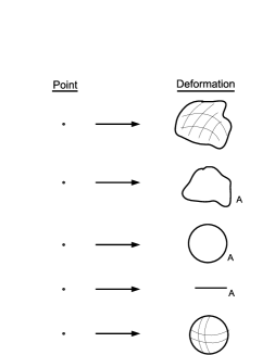
Figure 1: NS5-brane configurations in the continuous limit, their symmetries and the bosonic part of the operators driving the perturbation: (i) generic distribution in ${R}^{4}$ with no symmetry, (ii) generic planar deformation, (iii) circle (realizing a dilaton domain wall [6]), (iv) line segment , (v) 3-sphere. A and B label the planes where the branes are distributed (for planar distributions) and the one orthogonal to that, respectively. The vertex operator $e^{a\phi}$ has conformal dimension $\Delta=-{1\over 2}a(a+q)$.

$\@@underline{\hbox{Deformation of a finite size circle:}}$ In this case, depicted in fig. 2, the appropriate CFT is (1.5). Now the bosonic part of the perturbation is in terms of compact parafermions dressed with primaries of the non-compact part of the theory [4, 5]. The fermions enter through the bosons we use for their bosonization. The important new feature is that for finite $k$, there are no purely bosonic or fermionic terms. The clear semiclassical $\sigma$-model picture appears only in the limit $k\gg 1$. All the details can be found in [5].

Figure 2: On the left NS5-branes distributed on a circle of finite radius. They are deformed into the shape depicted on the right in the same plane. The symmetry is broken from $SO(2)_{A}\times SO(2)_{B}$ to $SO(2)_{B}$. The perturbation is driven by a chiral primary operator whose spin is related to the number of modes as $n=2(j+1)$.

3 Turning on angular momentum with CFT operators

The supergravity background corresponding to $k$ rotating NS5-branes was constructed in [13]. Quite a simplification occurs in the field-theory limit given by eqs. (14)-(17) of [13], where the interested reader can find the explicit form of the metric, the antisymmetric tensor and the dilaton fields. It was shown there that the Euclidean continuation of this background is obtained as an $O(3,3)$ transformation of the $SL(2,R)_{-k}/U(1)\times SU(2)_{k}$ CFT.

For vanishing rotation parameter $a_{i}$, $i=1,2$, this background becomes that in (1.3). The CFT operators driving it to the full solution are found by expanding the worldsheet Lagrangian density in the asymptotic region and keeping the first correction. For this we obtain the expression

$$\delta{\cal L}=\left[(a_{1}^{2}-a_{2}^{2})J^{3}_{+}J_{-}^{3}+\partial_{+}t\partial_{-}t+(a_{2}-a_{1})\partial_{+}tJ_{-}^{3}-(a_{1}+a_{2})J_{+}^{3}\partial_{-}t\right]e^{-q\phi}+{\cal O}\left(e^{-2q\phi}\right)\ ,$$ (3.1)

where the time $t$ is represented by a timelike free boson and

$$J^{3}_{\pm}=\sin^{2}\theta\partial_{\pm}\phi_{1}\pm\cos^{2}\theta\partial_{\pm}\phi_{2}\ ,$$ (3.2)

are chiral and antichiral (on shell) currents of the $SU(2)_{k}$ WZW model (generated by $\sigma_{3}$). The perturbation is clearly marginal and the dimension zero factor $e^{-q\phi}$ guarantees its normalizability. We also note that the first term in (3.1) is also responsible for spreading the NS5-branes from a point to a circle [6] (see, fig.1).

We conclude by mentioning that it remains to discuss systematically CFT deformations of the NS5 wold-volume. In that respect appropriate supergravity solutions have been constructed in [14].

References

- [1] M.J. Duff and J. X. Lu, Nucl. Phys. B354 (1991) 141.
- [2] C.G. Callan, J.A. Harvey and A. Strominger, Nucl. Phys. B359 (1991) 611.
- [3] K. Sfetsos, JHEP 9901 (1999) 015, arXiv:hep-th/9811167.
- [4] P.M. Petropoulos and K. Sfetsos, JHEP 0601 (2006) 167, arXiv:hep-th/0512251.
- [5] A. Fotopoulos, P.M. Petropoulos, N. Prezas and K. Sfetsos, JHEP 0802 (2008) 087, arXiv:0712.1912 [hep-th].
- [6] N. Prezas and K. Sfetsos, JHEP 0806 (2008) 080, arXiv:0804.3062 [hep-th].
- [7] P.M. Petropoulos, N. Prezas and K. Sfetsos, JHEP 0909 (2009) 085, arXiv:0905.1623 [hep-th].
- [8] O. Aharony, M. Berkooz, D. Kutasov and N. Seiberg, JHEP 9810 (1998) 004, arXiv:hep-th/9808149.
- [9] O. Aharony, B. Fiol, D. Kutasov and D. A. Sahakyan, Nucl. Phys. B679 (2004) 3, arXiv:hep-th/0310197.
- [10] O. Aharony, A. Giveon and D. Kutasov, Nucl. Phys. B691 (2004) 3, arXiv:hep-th/0404016.
- [11] C. Kounnas, M. Porrati and B. Rostand, Phys. Lett. 258B (1991) 61.
- [12] P.S. Howe and G. Sierra, Phys. Lett. 148B (1984) 451.
- [13] K. Sfetsos, Fortsch. Phys. 48 (2000) 199, arXiv:hep-th/9903201.
- [14] G. Papadopoulos, Class. Quant. Grav. 26 (2009) 135001, arXiv:0809.1156 [hep-th].