Coarse-Grained Simulations of Membranes under Tension

Abstract

We investigate the properties of membranes under tension by Monte-Carlo simulations of a generic coarse-grained model for lipid bilayers. We give a comprising overview of the behavior of several membrane characteristics, such as the area per lipid, the monolayer overlap, the nematic order, and pressure profiles. Both the low-temperature regime, where the membranes are in a gel $L_{\beta^{\prime}}$ phase, and the high-temperature regime, where they are in the fluid $L_{\alpha}$ phase, are considered. In the $L_{\beta^{\prime}}$ state, the membrane is hardly influenced by tension. In the fluid state, high tensions lead to structural changes in the membrane, which result in different compressibility regimes. The ripple state $P_{\beta^{\prime}}$, which is found at tension zero in the transition regime between $L_{\alpha}$ and $L_{\beta^{\prime}}$, disappears under tension and gives way to an interdigitated phase. We also study the membrane fluctuations in the fluid phase. In the low tension regime the data can be fitted nicely to a suitably extended elastic theory. At higher tensions the elastic fit consistently underestimates the strength of long-wavelength fluctuations. Finally, we investigate the influence of tension on the effective interaction between simple transmembrane inclusions and show that tension can be used to tune the hydrophobic mismatch interaction between membrane proteins.

I Introduction

Biological membranes are made of lipid bilayers with incorporated proteins. These barriers define the inside and the outside of a cell, separate the functional compartments in cells, and are indispensable for life Berg et al. (2002). The microscopic surface tension of membranes is usually small or vanishes altogether Nelson et al. (2004), but there may also be situations, where membranes are under considerable stress due to osmotic pressure differences. For example, epithelial cells exposed to transmembrane osmotic gradients can be expected to develop a state of tension under physiological conditions Soveral et al. (1997). Similarly, osmotically induced tension may play a decisive role during conformational changes, fission or fusion of cells Shillcock and Lipowsky (2005); Grafmüller et al. (2007). Another situation where membranes experience stress is under the influence of ultrasonic pulses Mitragotri (2005). Applied perpendicular to a lipid membrane, shock pulses can promote significant structural changes similar to those induced by lateral tension. The effect of such pulses on membranes is of considerable medical interest. In this context Koshiyama et al. have studied phospholipid bilayers under the action of a shock wave in atomistic molecular dynamics simulations Koshiyama et al. (2006).

Despite the advances in computer technology throughout the past decades, atomistic modeling of lipid bilayers on length scales of a few nanometer still requires huge computing resources or even goes beyond the current capabilities of high performance architectures. This motivates the use of coarse-grained models. They can give fundamental insights into the physics of a certain system, and, moreover, they provide powerful tools for the interpretation of the behavior of complex systems, like lipid membranes Voth (2009); Müller et al. (2006); Deserno (2009); Schmid (2009); Venturoli et al. (2006).

The aim of the work presented here is to study the effect of an externally applied tension on the physical properties of a model bilayer, and on the behavior of incorporated model proteins. We employ a generic coarse-grained model of amphiphiles developed in a top-down approachLenz and Schmid (2005). For tensionless systems this model has already been used very successfully to reproduce various bilayer phases including the symmetric and asymmetric ”rippled” $P_{\beta^{\prime}}$ states Lenz and Schmid (2007); West and Schmid (2010, in press) and to study membrane-protein interactions West et al. (2009). Recent simulations on membranes under mechanical stress have often dealt with the formation, structure and stability of hydrophilic pores Tileman et al. (2003); Leontiadou et al. (2004); Cooke and Deserno (2005) or with the influence of surface tension on transmembrane channel stability and function Gullingsrud and Schulten (2004); Zhu and Vaughn (2005). In this paper, we will primarily be concerned with the structural changes of pure membranes in response to lateral stresses, focussing on unporated systems. Since our model exhibits a rather realistic phase behavior of the model membrane at different temperatures, we can study different membrane states, i.e., the liquid, the ripple, and the gel state

Our paper is organized as follows: First we describe the underlying lipid model and outline the simulation methods. Then the simulation results are presented starting with a phenomenological introduction, where the effects of an external tension on the model bilayer in different phases are described. Thereafter a quantitative analysis of these bilayers is performed and the characteristics of the bilayers are examined with respect to their behavior under external tension. In the last part we show the influence of tension on the effective interaction potential of two simple model proteins. A brief summary concludes our paper.

II Model and Methods

In our model Schmid et al. (2007) the lipid molecules are represented by chains made of one head bead and six tail beads, and we have additional solvent beads. Hence we have three types of beads, $h,t$, and $s$ for head, tail, and solvent beads. Within the lipid chains, neighbor beads at a distance $r$ interact via a finite extensible non-linear elastic (FENE) potential

$$V_{\mathrm{FENE}}(r)=-\frac{1}{2}\epsilon_{\mathrm{FENE}}(\Delta r_{\mathrm{max}})^{2}\ln\left(1-\frac{(r-r_{0})^{2}}{\Delta r_{\mathrm{max}}^{2}}\right),$$ (1)

with the spring constant $\epsilon_{\mathrm{FENE}}$, the equilibrium bond length $r_{0}$, and the cutoff $\Delta r_{\mathrm{max}}$. The angles $\theta$ between subsequent bonds in the lipid are subject to a stiffness potential

$$V_{\textnormal{BA}}(\theta)=\epsilon_{\textnormal{BA}}(1-\cos\theta),$$ (2)

with the stiffness parameter $\epsilon_{\textnormal{BA}}$. Beads of type $i$ and $j$ which are not direct next neighbors in a chain interact via a truncated and shifted Lennard-Jones potential,

$$V_{\textnormal{LJ}}(r/\sigma_{ij})=\left\{\begin{array}[]{cl}\epsilon\left(\frac{\sigma_{ij}^{12}}{r^{12}}-2\frac{\sigma_{ij}^{6}}{r^{6}}\right)-V_{c,ij},&\textrm{if}\ r<r_{c,ij}\\ 0&\textrm{otherwise.}\end{array}\right.$$ (3)

The offset $V_{c,ij}$ is chosen such that $V_{\textnormal{LJ}}(r/\sigma_{ij})$ is continuous at the cutoff $r_{c,ij}$. The parameter $\sigma_{ij}=(\sigma_{i}+\sigma_{j})/2$ is the arithmetic mean of the diameters $\sigma_{i}$ of the interaction partners, and $r_{c,ij}=1\,\sigma_{ij}$ for all partners $(ij)$ except $(tt)$ and $(ss)$: $r_{c,tt}=2\,\sigma_{tt}$ and $r_{c,ss}=0$. Hence tail beads attract one another, all other interactions are repulsive, and solvent beads do not interact at all with each other. This way of modeling the solvent environment (the so-called ’phantom solvent’) Lenz and Schmid (2005) combines the advantages of explicit and implicit solvent models: Like implicit solvent models, the solvent environment does not develop any artificial internal structure, and it is very cheap (in Monte-Carlo or Brownian dynamics simulations, less than 10 % of the total computing time is spent on the solvent beads). Like explicit solvent models, the model can be used to study solvent-mediated phenomena such as the effect of hydrodynamic interactions on membrane dynamics. This is much more difficult with solvent-free models. We should note, however, that we mainly consider static membrane properties in the present work, using Monte-Carlo simulations.

We use the model parameters Schmid et al. (2007) $\sigma_{h}=1.1\,\sigma_{t}$, $r_{0}=0.7\,\sigma_{t}$, $\Delta r_{\mathrm{max}}=0.2\,\sigma_{t}$, $\epsilon_{\mathrm{FENE}}=100\,\epsilon/\sigma_{t}^{2}$, and $\epsilon_{\textnormal{BA}}=4.7\,\epsilon$. At the pressure $P=2.0\,\epsilon/\sigma_{t}^{3}$, the model reproduces the main phases of phospholipids, i.e., a high-temperature fluid $L_{\alpha}$ phase at temperature $k_{B}T>k_{B}T_{m}\sim 1.2\,\epsilon$ and a low-temperature tilted gel ($L_{\beta^{\prime}}$) with an intermediate modulated ripple ($P_{\beta^{\prime}}$) phase Lenz and Schmid (2007). The energy and length scales can be mapped to SI-units West et al. (2009) by matching the bilayer thickness or, alternatively, the area per lipid and the temperature of the main transition to those of DPPC, giving $1\,\sigma_{t}\sim 6\,\textrm{\AA}$ and $1\,\epsilon\sim 0.36\times 10^{-20}\,\mathrm{J}$. The elastic properties of the membranes in the fluid state were then also found to be comparable to those of DPPC membranes West et al. (2009).

Unless stated otherwise, the systems were studied by Monte-Carlo simulations at constant normal pressure $P_{N}=2.0\,\epsilon/\sigma_{t}^{3}$ and constant temperature $T$ with periodic boundary conditions in a simulation box of variable shape and size. We put the tension into effect by an additional energy term $-\Gamma A$ to the Hamiltonian of the system, where $A$ is the projected area of the bilayer onto the $xy$ plane. This alters the lateral components of the pressure tensor within the membrane. The non-interacting solvent particles, which probe the free volume and force the lipids to self-assemble, are not affected by this additional energy contribution. They ensure that the normal pressure $P_{N}$ is kept fixed at the required value. Thus, we are performing Monte-Carlo simulations in an $NP_{N}\Gamma\,T$ ensemble with effective Hamiltonian

$$H_{\mathrm{eff}}=E+P_{N}V-\Gamma A-Nk_{B}T\ln(V/V_{0})\quad,$$ (4)

where $E$ is the interaction energy, $V$ the volume of the simulation box, $V_{0}$ an arbitrary reference volume and $N$ the total number of beads. In contrast to the experimental situation, where the lateral pressure of a lipid bilayer cannot be controlled very easily Mouritsen (2005), our implementation of the tension is straightforward. Since we are in full control of the lateral pressure, we can gain insight into states and structures of lipid bilayers by means of computer simulations, which are difficult to investigate in experimental setups.

In practice, two main types of Monte-Carlo moves were proposed and then accepted or rejected according to a Metropolis criterion, namely 1) translational local moves of the beads, and 2) global moves which change the volume of the simulation box or its shape Schmid et al. (2007). During one Monte-Carlo step (MCS) there is on average one attempt to move each bead. Since the global moves require rescaling of all particle coordinates, which is rather expensive from a computational point of view, they are performed only every 50th MCS on average. The volume and shear moves are necessary to maintain the desired surface tension. An advantage of our scheme is that the correct area per lipid required by the external tension is adopted by construction. There is no need for searching the required state by testing various values of fixed area per lipid. We also implemented flip-flop moves with an inversion of the end-to-end vector of a complete lipid chain in its last tail bead, but found the acceptance rate of this ’molecular’ move due to the density of the bilayer far too small.

In some cases it turned out to be more convenient to keep the box height $L_{z}$ fixed and vary only the planar extension given by $L_{x}$ and $L_{y}$. In this case, the number of phantom solvent particles was allowed to fluctuate, i.e., additional Monte-Carlo moves were attempted where solvent particles were removed from the system or randomly inserted (semi-grand canonical simulations). The solvent chemical potential was set to

$$\mu_{s}=k_{B}\ln(V_{0}P_{N}/k_{B}T)\,.$$ (5)

Now, the semi-grand canonical Hamiltonian reads

$$H_{\mathrm{s,gc}}=E+P_{N}V-\Gamma A-\mu_{s}N_{s}-k_{B}T\ln\left[\left(V/V_{0})^{N}/N_{s}!\right)\right]\,,$$ (6)

where $N_{s}$ is the momentary number of solvent particles in the system.

When the system sizes were very large (Sec. III.4), the simulations were carried out on parallel processors using a domain decomposition scheme described in Ref. Schmid et al., 2007, which ensures that every Monte-Carlo move fulfills detailed balance exactly (in most other decomposition schemes proposed in the literature, detailed balance is violated at the boundaries between the domains). We have checked by comparison with single-processor simulations that the results were not affected by the parallelization.

In this paper the results presented in Section III.5 were obtained using the semi-grand canonical solvent model, and the diffusivity measurements (Sec. III.3) in the $NVT$-ensemble (in the latter case, only local bead translations were attempted and all simulations were run on a single processor). The other simulations used the $NP_{N}\Gamma\,T$-ensemble or.

The simulations of stressed membranes were carried out for a duration of at least $4\times 10^{6}\,\textnormal{MCS}$, and we checked that the observed quantities did not show any tendency for drift. In particular, we have examined in detail the long-wavelength undulations of the membranes, which are presumably the slowest relaxation modes in the system. After an equilibration time of $2\times 10^{6}\,\textnormal{MCS}$ the results from two successive runs of length $2\times 10^{6}\,\textnormal{MCS}$ were identical within the error. Hence the analyzed systems can be assumed to be in a stable state.

III Simulation Results

We have applied tensions of up to $\Gamma=3.0\,\epsilon/\sigma_{t}^{2}$, corresponding to $30\,\textrm{mN}/\textrm{m}$, which is close to the threshold for rupture in the fluid phase in our model: The membranes remained stable up to temperatures $k_{B}T=1.3\,\epsilon$, but ruptured at $k_{B}T=1.4\,\epsilon$ (see Fig. 1). This is consistent with atomistic simulations of Leontiadou et al., who found a critical tension for stable porated bilayers of $\approx 38\,\textrm{mN}/\textrm{m}$ in the context of pore formation with an atomistic model of DPPC Leontiadou et al. (2004). In contrast, the bilayer in the gel phase can sustain much higher tensions and stays stable for values of $\Gamma$ up to $4.0\,\epsilon/\sigma_{t}^{2}$ and higher. The areal expansion and reduction in thickness of the bilayer is substantial. In our simulations, we observe an increase in area per lipid of more than $40\,\%$ and a decrease in bilayer thickness of more than $30\,\%$ for high tensions, where the systems can still be found in non-rupturing configurations. In other simulation studies a comparable or even larger increase in the area per lipid was observed under tension without rupturing of the bilayer. Groot and Rabone report an areal expansibility of more than 70% for mixed membranes before these are finally ripped apart Groot and Rabone (2001). Grafmüller et al. see an areal gain of 60% under tension for one of their parameter sets Grafmüller et al. (2009).

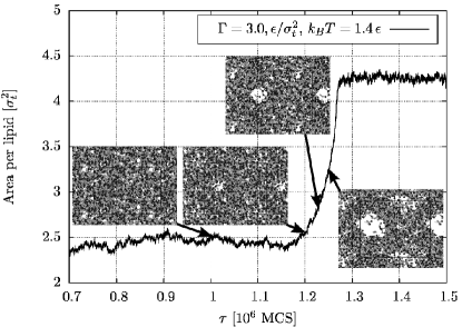
Figure 1: Snapshots (top view) of a rupture event at $k_{B}T=1.4\,\epsilon$ and $\Gamma=3.0\,\epsilon/\sigma_{t}^{2}$. The underlying curve shows the corresponding evolution of the area per lipid. At about $4.3\,\sigma_{t}^{2}$, the area per lipid levels off, because a restriction was imposed on the minimal size of the simulation box in the $z$ direction.

We begin with giving a qualitative overview over the behavior observed in the different bilayer phases. Figs. 2, 3, and 4 show configuration snapshots of bilayers under tension at the temperatures $k_{B}T=1.3\,\epsilon$, corresponding to a fluid state, $k_{B}T=1.2\,\epsilon$, corresponding to a rippled state, and $k_{B}T=1.1\,\epsilon$, corresponding to a tilted gel state.

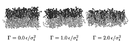
Figure 2: Snapshots of bilayer configurations in the fluid phase at $k_{B}T=1.3\,\epsilon$. Gray scale coding: Light gray molecules point upwards from head to tail, dark gray molecules point downwards. At increasing tension the two monolayers partly interdigitate. The size of the beads are not to scale.

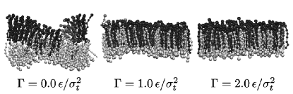
Figure 3: Snapshots of bilayer configurations in the ripple phase at $k_{B}T=1.2\,\epsilon$ (gray scale coding as in Fig. 2). On the left the tensionless system with a pronounced ripple is depicted. This ripple vanishes as tension is applied, giving way to a completely interdigitated structure (middle and right figure).

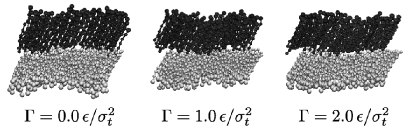
Figure 4: Snapshots of bilayer configurations in the gel phase $k_{B}T=1.1\,\epsilon$ (gray scale coding as in Fig. 2). No interdigitation at increasing tension is observed.

In the fluid phase (Fig. 2), the membrane stretches under tension, and the two monolayer leaflets become less well separated (right). Thus high tensions change the structure of the membrane. This effect is even more pronounced in the rippled state (Fig. 3; here the original rippled structure was obtained by cooling tensionless equilibrated configurations from the fluid phase at $k_{B}T=1.3\,\epsilon$ down to $k_{B}T=1.2\,\epsilon$). Under tension, the ripple unravels and gives way to an interdigitated phase. In contrast, the gel state (Fig. 4) is hardly affected under tension. The two monolayers remain well-separated. Only the average lipid tilt away from the bilayer normal is slightly enhanced from $\langle\theta\rangle=23^{\circ}$ in the tensionless state to $\langle\theta\rangle=30^{\circ}$ at the tension $\Gamma=3.0\,\epsilon/\sigma_{t}^{2}$ (snapshot not shown).

After this qualitative overview, we turn to a more quantitative analysis of the behavior of bilayers under tension.

III.1 Global characteristics of pure membranes

We first consider the area per lipid, which is obtained by dividing the projected area of the bilayer in the $xy$ plane by half the number of lipids in the system. We note that the difference between the number of lipids in the upper and the lower monolayer was always very small. ”Flip-flop” moves are practically never observed for systems in the gel phase. In the fluid phase, about $10\,\%$ of the lipids were exchanged between the monolayers during $10^{6}\,\textnormal{MCS}$, but fluctuations of the average number of lipids in each monolayer are still less than $2\,\%$.

We do not observe any dependence of the area per lipid on the system size. For the temperature $k_{B}T=1.3\,\epsilon$, we have compared data from four different system sizes, ranging from $200$ lipids to $7,200$ lipids; the results were identical within the statistical error ($\approx 1\,\%$). These results are in agreement with the findings of Marrink and Mark in atomistic simulations Marrink and Mark (2001), or with those of Kranenburg et al. Kranenburg et al. (2003), who studied a coarse-grained model of amphiphilic surfactants by a combined DPD and Monte-Carlo scheme, imposing the surface tension in a way similar to ours.

Assuming that the area per lipid $A$ depends linearly on the applied tension $\Gamma$, one can calculate the mean area compressibility modulus $k_{A}$ using the relation $k_{A}=A_{0}{\Delta\Gamma}/{\Delta A},$ where $A_{0}$ is the equilibrium area of the tensionless membrane. This yields the values of $k_{A}$ listed in Table 1. Here only data from configurations which remained stable for long simulation runs (up to $10^{7}\,\textnormal{MCS}$) have been taken into consideration, i.e., the data for the state point $k_{B}T=1.4\,\epsilon$, $\Gamma=3.0\,\epsilon/\sigma_{t}^{2}$, which lies beyond the rupture threshold, were omitted.

$k_{B}T$ [$\epsilon$]	1.0	1.1	1.3	1.4
$k_{A}$ [$\epsilon/\sigma_{t}^{2}$]	40	32	4.3	4.6

Table 1: Mean area compressibility modulus $k_{A}$ over the whole range of tensions.

For membranes in the gel phase ($k_{B}T=1.0\,\epsilon$ and $k_{B}T=1.1\,\epsilon$), the number $k_{A}$ fully characterizes the behavior of the area per lipid over the whole investigated range of tensions (data not shown). The extensibility of the bilayer in the gel phase is significantly smaller than in the fluid phase, and constant over the whole range of tensions under investigation. The most noticeable effect of the tension is the increase in tilt angle of the lipids mentioned earlier, which leads to a slightly reduced membrane thickness.

The behavior of membranes in the fluid or ripple state is more complicated. Fig. 5 shows the corresponding data for the area per lipid as a function of the applied tension.

We first discuss the situation at the temperature $k_{B}T=1.2\,\epsilon$, where the tensionless membrane is in the ripple phase. As we have already discussed earlier (Fig. 3), the membrane undergoes a phase transition to an interdigitated phase under tension. Fig. 5, top, shows that this is associated with a pronounced change of the compressibility. Up to values of about $1.0\,\epsilon/\sigma_{t}^{2}$, the area per lipid increases steeply, the resulting value of $k_{A}$ is even lower than that of the fluid phase. At high tensions, $\Gamma=1.9\,\epsilon/\sigma_{t}^{2}$ and above, the approximate areal compressibility is strongly enhanced and comparable to values obtained for systems in the gel phase. Thus the extensibility of the bilayer changes from fluid-like to gel-like under tension.

In the fluid phase (Fig. 5, bottom), the tension-induced structural changes in the membranes are less dramatic, but they can still be associated with compressibility changes. The data shown in Fig. 5, bottom, suggest a subdivision into three different compressibility regimes: Under tension, the membrane switches from a less compressible low-tension state to a more compressible high-tension state via a highly compressible intermediate. Thus the structural changes in the membrane, which were observed in Fig. 2, seem to be related to a crossover between different membrane states and possibly even reflect the vicinity of a hidden phase transition.

The inset in Fig. 5, bottom, focuses on the limit of very small tension/compression. In recent work, $k_{A}$ has been determined for the case $\Gamma=0.0\,\epsilon/\sigma_{t}^{2}$ with an alternative method, i.e., the detailed analysis of the fluctuation spectrum of tensionless membranes West et al. (2009). Here, we have extracted the areal compressibility modulus of the fluid membrane close to tension zero by both compressing and extending the system slightly within the range of $\Gamma=-0.2$ to $0.2\,\epsilon/\sigma_{t}^{2}$. The resulting value for $k_{A}$ divided by the square of the mean tensionless monolayer thickness $t_{0}\approx 3\,\sigma_{t}$ agrees with the value $k_{A}/t_{0}^{2}=1.1\pm 0.2\,\epsilon/\sigma_{t}^{2}$ obtained independently from the fluctuation analysis (see Table 2).

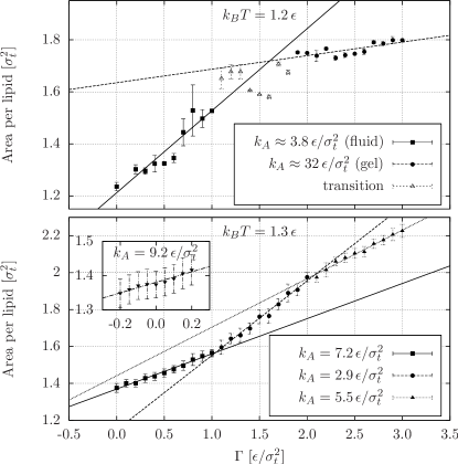
Figure 5: Area per lipid $A$ vs. tension $\Gamma$ for two different temperatures as indicated, together with linear fits to different compressibility regimes.
Top: As the tension on a patch of bilayer in the ripple-phase increases, the areal compressibility changes from fluid-like to gel-like.
Bottom: In the fluid phase, three different compressibility regimes are observed, $\Gamma=0$–$1\,\epsilon/\sigma_{t}^{2}$, $\Gamma=1$–$2\,\epsilon/\sigma_{t}^{2}$, and $\Gamma=2$–$3\,\epsilon/\sigma_{t}^{2}$. The inset focuses on the tensionless membrane (see text for explanation)

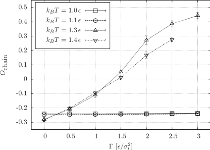
Figure 6: Average overlap parameter (see text for definition) vs. tension. Negative values indicate spatially well-separated monolayers. For interdigitated bilayers the overlap parameter is positive.

To characterize the global structure of the membrane in more detail, we next consider the interdigitation of the two monolayers. It can be characterized in terms of the ’overlap parameter’ $O_{\textrm{chain}}=\langle 2(l_{z}-t_{0})/l_{z}\rangle$, originally introduced by Kranenburg et al. Kranenburg et al. (2003). The results are shown in Fig. 6. They quantify the behavior which was already apparent from the snapshots shown earlier (Figs. 2–4). In the gel phase, where we did not notice any overlap of the monolayers even under tension $O_{\textrm{chain}}$ is always negative. In the fluid phase, it becomes positive at high tensions.

Interestingly, this leads to a non-monotonic behavior of the orientational chain order in the fluid phase, i.e., the nematic order parameter $S_{z}=1/2\langle(l_{z}/l)^{2}-1\rangle$. Here, $l_{z}$ is again the $z$ component of the end-to-end vector of a lipid chain, and $l$ its full length. As shown in Fig. 7, the nematic order first decreases in the low-tension regime $\Gamma<1.0\,\epsilon/\sigma_{t}^{2}$. At $\Gamma\sim 1.5-2.0\,\epsilon/\sigma_{t}^{2}$, a rather steep increase ensues, followed by a plateau in the high-tension regime $\Gamma>2.0\,\epsilon/\sigma_{t}^{2}$. Under tension, the lipids thus first disorder and tilt away from the bilayer normal, which leads to an unfavorable packing in the hydrophobic bulk of the membrane. As interdigitation sets in, the lipids relax and assume once again their preferred order.

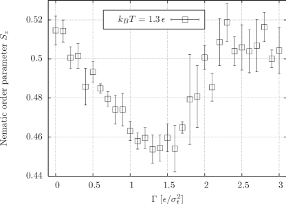
Figure 7: Nematic order parameter of chains $S_{z}$ vs. tension.

III.2 Pressure Profiles

After having discussed these global properties of the membranes, we now investigate the effect of the applied external stress on the internal stress distribution inside the membrane. Stress distribution profiles influence, e.g., the permeability of membranes with respect to small molecules. To study them, we have recorded the interfacial tension (or negative stress) profiles

$$\gamma(z)=P_{zz}(z)-\frac{1}{2}(P_{xx}(z)+P_{yy}(z))$$ (7)

in small systems of 200 lipids. The pressure tensor $P_{\alpha\beta}$ is obtained using the virial theorem,

$$P_{\alpha\beta}=\frac{Nk_{B}T}{V}\delta_{\alpha\beta}+\frac{1}{V}\left\langle\sum_{i}r_{i}^{\alpha}F_{i}^{\beta}\right\rangle.$$ (8)

Here, $\mathbf{r}_{i}$ is the position of particle $i$, $\mathbf{F}_{i}$ the force acting on this particle, $N$ the number of particles, $T$ the temperature, and $V$ the volume. The local distribution of the pressure along the bilayer normal was obtained by dividing the system into 50 vertical slabs and distributing the pressure contributions onto these slabs according to the convention of Irving and Kirkwood Irving and Kirkwood (1950). The pressure profiles can also be used to cross-check the consistency of our approach in Eq. 4, since the integral

$$\Gamma_{0}=\int\mathrm{d}z\>\gamma(z)$$ (9)

has to match the externally applied tension. We have checked that this was the case in all simulations.

Pressure or stress profiles have been reported in various other studies Goetz and Lipowsky (1998); Brannigan et al. (2006); Gullingsrud and Schulten (2004) for both mesoscopic and atomistic simulations. We will briefly summarize the characteristic features of the total stress profiles and analyze their change under tension in our model. The behavior of the pressure profiles can be attributed to different interactions:

The first positive peak (insets in Figures 8 and 9) arises due to the purely repulsive interactions of the head and the solvent beads. Here a zone depleted from (solvent) beads is formed and the head beads are effectively squeezed together in the lateral direction. The first negative peak in the head region indicates that the head-head interactions are purely repulsive, pushing the system laterally apart in this section of the bilayer. The second positive peak, located in the tail region, results from the interplay of the attractive Lennard-Jones interaction between the tail beads and the contribution of bond-angle and bond-length potentials. Interestingly, the contribution of the (attractive) Lennard-Jones (LJ) interactions between tail beads is negative: The net attraction between tail beads is stronger in the normal direction than in the lateral direction. This is compensated and outbalanced by the contributions of the bending of the lipid segments and the stretching of bonds, which lead to positive tension in total. Thus the stress in the hydrophobic portion of the membrane is mostly sustained by intrachain interactions and not, as one might expect, by the attractive Lennard-Jones interactions. The negative peak in the midplane of the bilayer originates from the absence of intrachain interactions in this region, thus the effect of the Lennard-Jones interactions takes over and the monolayers are effectively glued to each other.

Under the influence of an external tension, we observe a narrowing and shift of the whole profiles, in qualitative agreement with previous atomistic simulations by Gullingsrud and Schulten Gullingsrud and Schulten (2004). In the gel phase, which is already exposed to very high internal stress, the relative effect of the external tension is small. The inspection of the different contributions to the local pressure shows that the external tension leads to a decrease both of the Lennard-Jones (LJ) contribution and the bond length (BL) contribution. The reduction of the LJ-contribution is higher, leading to the observed shift. Due to the stiffness of the lipids in the gel phase, the bond-angle contribution to the pressure profiles remains practically unaltered. The change in the overall structure of the pressure profiles is also only small. The slight change in membrane thickness results in a shift of the outer peaks of the profiles towards the midplane ($z=0$).

The effect of external tension is considerably more dramatic in the fluid phase at $k_{B}T=1.3\,\epsilon$. Although the absolute peak values of the pressure profiles are reduced by a factor of about 8 to 10, the relative shifts are much more pronounced. First, the shift of the outermost peaks towards the midplane is much higher, due to the fact that the membrane thickness decreases more strongly under tension in this phase. Second, the shapes of the individual contributions to the total profile change qualitatively under stress, reflecting the structural change from a well-separated bilayer to an interdigitated structure. At high $\Gamma$, the individual terms have a simple structure with single, positive or negative, peaks at the center of the membrane. Nevertheless, the total stress profile still exhibits the oscillatory features described above.

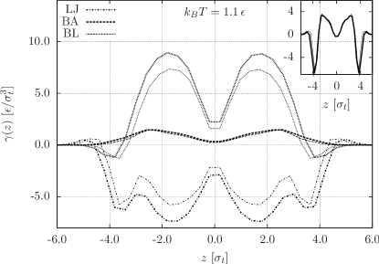
Figure 8: Contributions of the Lennard-Jones (LJ), bond-angle (BA), and bond-length (BL) interactions to the total stress profiles in the gel phase, for the tensionless case (thick lines) and for the tension $\Gamma=2.0\,\epsilon/\sigma_{t}^{2}$ (thin lines). The inset shows the total stress profile, i.e., the sum of all contributions, for $\Gamma=0.0\,\epsilon/\sigma_{t}^{2}$ (thick line) and $\Gamma=2.0\,\epsilon/\sigma_{t}^{2}$ (thin line).

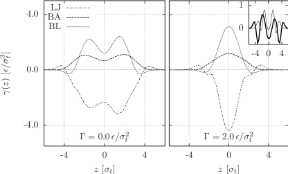
Figure 9: Contributions of the Lennard-Jones (LJ), bond-angle (BA), and bond-length (BL) interactions to the total stress profiles in the fluid phase, in the tensionless case (left), and for the tension $\Gamma=2.0\,\epsilon/\sigma_{t}^{2}$ (right). The inset shows the total stress profile for the tensionless bilayer (thick line) and for $\Gamma=2.0\,\epsilon/\sigma_{t}^{2}$ (thin line).

III.3 Correlation functions and diffusion of lipids

Next we consider the effect of the tension on the lateral structure of the bilayers and on the dynamic mobility of individual lipids. Fig. 10 shows the two-dimensional radial distribution function $g_{m}(r)$ of the $(x,y)$-coordinates of the head groups in the gel and the fluid state for different applied tensions $\Gamma$. In the gel state, $g_{m}(r)$ exhibits a series of pronounced peaks, reflecting a high degree of order (Fig. 10, left). Under tension, the higher order peaks shift to slightly larger distances, reflecting the enhancement of the area per lipid. The fluid membrane is much less structured. The head-head radial correlation functions within one monolayer decay rapidly already at zero tension, and all higher order peaks disappear at higher tension (Fig. 10, right). In sum, the influence of the tension on the lateral structure of the membranes is found to be largely negligible.

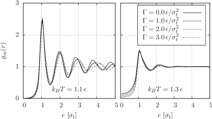
Figure 10: Two-dimensional radial distribution function $g_{m}(r)$ of the head groups within one monolayer at $k_{B}T=1.1\,\epsilon$ (left) and at $k_{B}T=1.3\,\epsilon$ (right).

The situation is different for the diffusion coefficient of lipids. Although Monte-Carlo simulations do not provide an intrinsic timescale, one can still obtain valuable information on the diffusional behavior of the lipids from $NVT$ Monte-Carlo simulations that employ only local bead moves. In our diffusivity studies, the initial configurations were taken from systems equilibrated in the $NP_{N}\Gamma\,T$-ensemble, but we measured the diffusivity of lipids in the $NVT$-ensemble, i.e., no volume or shear moves were carried out during the simulation. We have monitored the pressure tensor for the duration of the diffusion measurements to check that it stayed constant during the simulation.

In the following, the basic ”time unit” is one Monte-Carlo step (MCS, the Monte-Carlo ’time scale’), and the ”time” $\tau$ counts the number of MCS since the start of the simulation. We consider the lateral diffusion constant within the membrane (or, more specifically, the projection of the membrane into the ($xy$ plane)), defined as Goetz and Lipowsky (1998)

$$D_{xy}(\tau)=\frac{\sum_{i}\left(\sum_{t=0}^{\tau}\Delta\mathbf{r}_{i}^{(xy)}(t)\right)^{2}}{6N\tau}\,.$$ (10)

Here the sum $i$ runs over all lipid heads, $\mathbf{r}_{i}^{(xy)}$ denotes the position of a lipid head $i$ in the $xy$ plane with respect to the center of mass of the bilayer, and $\Delta\mathbf{r}_{i}^{(xy)}$ its difference from one MCS time step to the next without the offset that has to be added if the head crosses the periodic boundaries.

In the gel phase (data not shown), no diffusion was observed over the whole length of the simulation ($\tau_{\textnormal{max}}=1.2\times 10^{7}\,\textnormal{MCS}$). The lipids basically fluctuate around their average positions. The width of the fluctuations, $\sqrt{\langle{r^{(xy)}}^{2}\rangle-\langle\mathbf{r}^{(xy)}\rangle^{2}}\sim 0.04\,\sigma_{t}$, does not depend on the applied tension. The data for the fluid phase are shown in Fig. 11. Here the lipids diffuse freely, and the lateral diffusion constant $D_{xy}$ increases significantly if one applies moderate tensions up to $\Gamma=2.0\,\epsilon/\sigma_{t}^{2}$ (Fig. 11). Interestingly, it does not increase further in the high-tension regime, beyond $\Gamma=2.0\,\epsilon/\sigma_{t}^{2}$, even though the area per lipid and the chain overlap parameter $O_{\textrm{chain}}$ are not yet saturated.

It should be noted that the in-plane diffusion constant discussed here differs from the true diffusion constant in the membrane, due to the presence of membrane undulations (see also Sec. III.4). The thermally induced buckling of the membrane can lead to a substantial out-of-plane component to the lipids’ diffusional motion, which is not captured in our definition of $D_{xy}$ in Eq. 10. Various theoretical studies have addressed this problem Gustafsson and Halle (1997); Naji and Brown (2007); Reister-Gottfried et al. (2007). They commonly conclude that membrane fluctuations lower the measured in-plane diffusion coefficient. As the tension increases, the fluctuations of the membrane are suppressed (see Sec. III.4). Therefore, one may speculate that the increase of the apparent diffusivity under tension measured in our simulations is, at least in part, caused by the reduction of thermal bilayer undulations. However, this is not sufficient to fully explain the 20%-effect observed in Fig. 11.

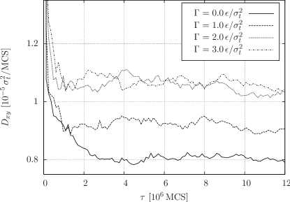
Figure 11: Lateral diffusion coefficient $D_{xy}$ for different tensions $\Gamma$.

III.4 Fluctuation spectra

To conclude the analysis of pure membranes, we study the thermal membrane fluctuations, which were already mentioned in the previous section. Theoretical considerations Helfrich (1978) and experiments Israelachvili and Wennerström (1992) have shown that lateral tension on fluid bilayers leads to suppression of thermal fluctuations, which in turn decreases steric repulsion of vesicles and changes adhesive properties. Moreover, the Fourier spectra of the height and thickness fluctuations provide information on the elastic properties of the membranes. Therefore, it is instructive to look at the development of undulation, peristaltic and protrusion properties of our model membrane under tension.

To analyze our data, we use an extension of an elastic theory by Brannigan and Brown Brannigan and Brown (2006), which we have already applied with success to the case of the tensionless membrane West et al. (2009). We shall not rederive the theory here, but merely sketch the main assumptions. Brannigan and Brown describe a planar fluctuating membrane as a system of two coupled monolayers surfaces $h_{1,2}(x,y)$, of with each is characterized by two independent fields, $z_{1,2}(x,y)$ and $\lambda_{1,2}(x,y)$ ($h=z+\lambda$), one accounting for slow ’bending modes’ and one for fast ’protrusion modes’Götz et al. (1999). They furthermore make a number of approximations, which amount to the assumptions that

• the protrusion modes of the two monolayers are independent degrees of freedom,

• the bending modes $z_{1,2}(x,y)$ can be rewritten in terms of their sum and their difference ($z_{\pm}=(z_{1}\pm z_{2})/2$), corresponding to (bending) height and (bending) thickness modes of the membrane, which in turn decouple. The (bending) thickness modes are subject to the constraint that the volume per lipid is conserved.

With these assumptions, Brannigan and Brown construct a free energy functional which is quadratic in the fluctuations of the fields $z$ and $\lambda$ (higher order contributions are neglected) and can be used to calculate the thermally averaged fluctuations of the total membrane height, $h=(h_{1}+h_{2})/2$, and monolayer thickness, $t=(h_{1}-h_{2})/2$.

In our simulations, the situation is different from that considered by Brannigan and Brown in two respects. First, we apply an external tension. Second, we do not have well-separated monolayers, especially at high tensions. We argue that the second point is not critical: If we associate the fields $h_{1,2}$ with the positions of the head group layers layers rather than whole monolayers, the assumptions enumerated above are still reasonable and we obtain the same theory. The first point is more subtle, since the external tension is not an intrinsic material parameter such as, e.g., the bending energy (which drives the bending fluctuations).

To assess the effect of an applied external tension on the height fluctuations, we first consider a simplified case, where the membrane is characterized by a single surface manifold $h(x,y)$ (shifted to $\langle h\rangle=0$) with fixed surface area $A_{s}$ and variable projected area $A$. The surface area is related to the projected area via

$$A_{s}=\int_{A}\mathrm{d}^{2}r\sqrt{1+(\nabla h)^{2}}\approx A+\frac{1}{2}\int\mathrm{d}^{2}r(\nabla h)^{2}\,.$$ (11)

Upon applying an external tension $\Gamma$, the free enthalpy $G$ of the system is given by

$$G=-\Gamma A\approx-\Gamma A_{s}+\frac{\Gamma}{2}\int\mathrm{d}^{2}r\>(\nabla h)^{2},$$ (12)

where $\Gamma A_{s}$ is a constant. Hence the external tension couples to the fluctuations of the local membrane height $h(x,y)$ in the same way as an internal interfacial tension couples to the fluctuations, e.g., a gas-liquid interface Rowlinson and Widom (1982).

The same type of argument can be applied to the model of Brannigan and Brown, where the membrane has finite thickness and the lipid volume, rather than the lipid area, is conserved: Let $z_{+}(x,y)$ and $2z_{-}(x,y)$ denote the local membrane height and thickness as before, with $\langle z_{+}\rangle=0$. Let furthermore $D(x,y)$ denote the true local membrane thickness, evaluated with respect to the local surface normal, i.e., $z_{-}(x,y)=D\sqrt{1+(\nabla z_{+})^{2}}/2$. The thickness is taken to fluctuate weakly about its mean value $\overline{D}$, i.e., $D(x,y)=\overline{D}+\delta(x,y)$. The number of lipids on the projected area element $\mathrm{d}A$ is then given by

$$N = \frac{2}{v}\int_{A}\textnormal{d}^{2}r\>z_{-}=\frac{1}{v}\int_{A}\mathrm{d}^{2}r\>\sqrt{1+(\nabla z_{+})^{2}}\>D$$ (13)

$$\approx \frac{1}{v}\left(\overline{D}A+\frac{\overline{D}}{2}\int\mathrm{d}^{2}r(\nabla h)^{2}+\int\mathrm{d}^{2}r\>\delta\right)$$

with the lipid volume $v$, where we have expanded up to second order in the fluctuating fields $h$ and $\delta$. Upon applying an external tension $\Gamma$, the free enthalpy acquires an additional term

$$G_{\Gamma}=-\Gamma A=-\frac{\Gamma vN}{\overline{D}}+\frac{\Gamma}{2}\int_{A}\mathrm{d}^{2}r(\nabla z_{+})^{2}+\frac{\Gamma}{\overline{D}}\int\mathrm{d}^{2}r\>\delta,$$ (14)

where $\Gamma vN/\overline{D}=\mbox{const.}$ Hence the external tension again has the same effect on the height fluctuations than an internal tension. The last term in Eq. (14) results in an effective thinning of the membrane and does not contribute to the fluctuation spectra in the quadratic order considered here.

Supplementing the free energy of Brannigan and Brown Brannigan and Brown (2006) with this additional tension term, we obtain the Hamiltonian (in Fourier space)

$$\begin{split}F=&\frac{1}{2}\sum_{\mathbf{q}}(k_{c}q^{4}+\Gamma q^{2})z_{\mathbf{q}}^{+}z_{\mathbf{-q}}^{+}\\ &+2(k_{\lambda}+\gamma_{\lambda}q^{2})\lambda_{\mathbf{q}}^{+}\lambda_{\mathbf{-q}}^{+}\\ +&\frac{1}{2}\sum_{\mathbf{q}}(k_{A}/t_{0}^{2}+k_{c}q^{4}-4k_{c}\zeta q^{2}/t_{0})z_{\mathbf{q}}^{-}z_{\mathbf{-q}}^{-}\\ &+2(k_{\lambda}+\gamma_{\lambda}q^{2})\lambda_{\mathbf{q}}^{-}\lambda_{\mathbf{-q}}^{-}\quad.\end{split}$$ (15)

Here $z^{\pm}$ denotes the bending modes defined above, and $\lambda^{\pm}=(\lambda_{1}\pm\lambda_{2})/2$ the corresponding protrusion modes. The parameters $k_{c}$ and $k_{A}$ are the bending and compressibility moduli of the bilayer, $\zeta$ is related to the spontaneous curvature $c_{0}$ and given by $c_{0}-\Sigma\>\textrm{d}c_{0}/\textrm{d}\Sigma$ with the area per lipid $\Sigma$, $t_{0}$ is the mean monolayer thickness, and the parameters $\gamma_{\lambda}$ and $k_{\lambda}$ characterize the protrusion modes. The resulting spectra for height and thickness fluctuations are given by

$$\langle|h_{\mathbf{q}}|^{2}\rangle=\frac{k_{B}T}{k_{c}q^{4}+\Gamma q^{2}}+\frac{k_{B}T}{2(k_{\lambda}+\gamma_{\lambda}q^{2})}\\$$ (16)

$$\langle|t_{\mathbf{q}}|^{2}\rangle=\frac{k_{B}T}{k_{c}q^{4}-4k_{c}\zeta q^{2}/t_{0}+k_{A}/t_{0}^{2}}+\frac{k_{B}T}{2(k_{\lambda}+\gamma_{\lambda}q^{2})}\quad.$$ (17)

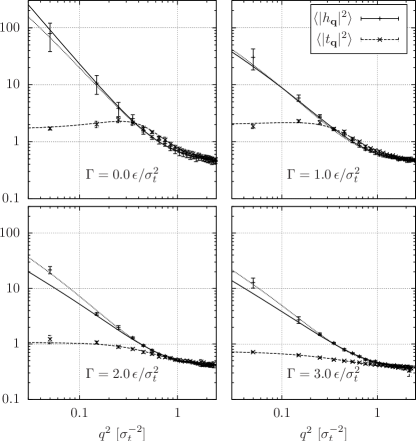
Figure 12: Fluctuation spectra of membranes for different tensions as indicated. The dashed line is the fit to the thickness spectrum. The solid line shows the fit of the elastic theory to the height spectrum for fixed tension $\Gamma$ and the dotted line shows the fit with $\Gamma_{\textrm{fit}}$ as additional fit parameter. At higher tensions these fits deviate from each other. The values of $\Gamma_{\textrm{fit}}$ are listed in Table 3.

We have determined the fluctuation spectra from simulations of systems containing 3,200 lipids and 24,615 solvent beads using a method described elsewhere Loison et al. (2003); West et al. (2009), and used the theory above to fit our data. As in our earlier work West et al. (2009), the fitting yields very good results for tensionless membranes. It still works well at the comparatively low tension of $\Gamma=1.0\,\epsilon/\sigma_{t}^{2}$. In the high-tension regime above $2.0\,\epsilon/\sigma_{t}^{2}$ , however, the situation changes. When fixing $\Gamma$ to the externally applied value, the fit consistently underestimates the amplitudes of the long-wavelength fluctuations. This can be remedied by leaving $\Gamma$ as fit parameter. However, the resulting values for the fitted tension are smaller by a factor of up to one half than the externally applied values (Fig. 12). The fit parameters for the fits with fixed and free parameter $\Gamma$ are given in Tables 2 and 3.

$\Gamma$ [$\epsilon/\sigma_{t}^{2}$]	0.0	1.0
$k_{c}$ [$\epsilon$]	$4.9\pm 1.0$	$6.2\pm 0.5$
$\zeta/t_{0}$ [$\sigma_{t}^{-2}$]	$0.12\pm 0.02$	$0.069\pm 0.019$
$k_{A}/t_{0}^{2}$ [$\epsilon/\sigma_{t}^{4}$]	$1.1\pm 0.2$	$0.92\pm 0.09$
$k_{\lambda}$ [$\epsilon/\sigma_{t}^{4}$]	$1.4\pm 0.1$	$1.4\pm 0.1$
$\gamma_{\lambda}$ [$\epsilon/\sigma_{t}^{2}$]	$0.022\pm 0.039$	$0.035\pm 0.021$
$\Gamma$ [$\epsilon/\sigma_{t}^{2}$]	2.0	3.0
$k_{c}$ [$\epsilon$]	$7.0\pm 0.3$	$7.7\pm 0.3$
$\zeta/t_{0}$ [$\sigma_{t}^{-2}$]	$-0.038\pm 0.008$	$-0.137\pm 0.040$
$k_{A}/t_{0}^{2}$ [$\epsilon/\sigma_{t}^{4}$]	$1.8\pm 0.2$	$4.0\pm 0.4$
$k_{\lambda}$ [$\epsilon/\sigma_{t}^{4}$]	$1.8\pm 0.1$	$2.0\pm 0.1$
$\gamma_{\lambda}$ [$\epsilon/\sigma_{t}^{2}$]	$-0.048\pm 0.042$	$-0.062\pm 0.048$

Table 2: Elastic parameters of the model membrane in the fluid phase, obtained from a fit of the elastic theory (Eqs. 16 and 17) with fixed $\Gamma$.

$\Gamma$ [$\epsilon/\sigma_{t}^{2}$]	0.0	1.0
$k_{c}$ [$\epsilon$]	$4.4\pm 0.7$	$6.6\pm 0.9$
$\zeta/t_{0}$ [$\sigma_{t}^{-2}$]	$0.11\pm 0.02$	$0.074\pm 0.019$
$k_{A}/t_{0}^{2}$ [$\epsilon/\sigma_{t}^{4}$]	$1.0\pm 0.2$	$0.95\pm 0.11$
$k_{\lambda}$ [$\epsilon/\sigma_{t}^{4}$]	$1.5\pm 0.1$	$1.4\pm 0.1$
$\gamma_{\lambda}$ [$\epsilon/\sigma_{t}^{2}$]	$0.018\pm 0.043$	$0.041\pm 0.026$
$\Gamma_{\textrm{fit}}$ [$\epsilon/\sigma_{t}^{2}$]	$0.11\pm 0.19$	$0.83\pm 0.14$
$\Gamma$ [$\epsilon/\sigma_{t}^{2}$]	2.0	3.0
$k_{c}$ [$\epsilon$]	$10.9\pm 0.8$	$12.6\pm 1.1$
$\zeta/t_{0}$ [$\sigma_{t}^{-2}$]	$-0.011\pm 0.012$	$-0.11\pm 0.08$
$k_{A}/t_{0}^{2}$ [$\epsilon/\sigma_{t}^{4}$]	$2.0\pm 0.3$	$4.3\pm 0.5$
$k_{\lambda}$ [$\epsilon/\sigma_{t}^{4}$]	$1.6\pm 0.03$	$1.7\pm 0.1$
$\gamma_{\lambda}$ [$\epsilon/\sigma_{t}^{2}$]	$0.057\pm 0.030$	$0.048\pm 0.032$
$\Gamma_{\textrm{fit}}$ [$\epsilon/\sigma_{t}^{2}$]	$0.90\pm 0.31$	$1.7\pm 0.4$

Table 3: Elastic parameters of the model membrane in the fluid phase from a fit to Eqs. 16 and 17 where the parameter $\Gamma$ is allowed to vary. The fitted value is $\Gamma_{\textrm{fit}}$.

The relation between external ($\Gamma$) and internal stress ($\Gamma_{\textnormal{int}}$) in membranes has been discussed by a number of authors for the situation where the membrane is kept in a frame with fixed projected area $A$. In these studies, the total area $A_{s}$ was allowed to fluctuate, either because of fluctuations in the number of molecules (grandcanonical case) Cai et al. (1994); Farago and Pincus (2003) or because of fluctuations of the lipid area (canonical, compressible case) Farago and Pincus (2003); Imparato (2006). The frame tension is then found to differ from the internal stress in the membranes due to the contribution of the membrane fluctuations to the surface free energy Brochard et al. (1976); David and Leibler (1991); Cai et al. (1994); Farago and Pincus (2003); Imparato (2006). The correction is additive and should always be present, even at (external or internal) tension zero. For the canonical, compressible case, which is obviously more relevant in our context, Farago et al. Farago and Pincus (2003) and Imparato Imparato (2006) have predicted that the fluctuations reduce the frame tension by roughly $k_{B}T\,n/A$, compared to the intrinsic stress, where $n$ is the number of fluctuation degrees of freedom, i.e., the number of independently fluctuating membrane patches. Thus the intrinsic tension should be higher than the frame tension, which is opposite from what we observe in our simulations.

However, we believe that the two situations – fixed frame and varying surface area versus variable frame and (roughly) fixed surface area – are not comparable. According to the arguments leading to Eqs. (12) and (14), the frame tension is not renormalized by fluctuations at the level of a Gaussian theory (i.e., a theory based on a free energy functional which is quadratic in the fluctuations). It might be renormalized if one includes higher order terms. For example, the last term in Eq. (14), $\propto\int\mathrm{d}^{2}r\>\delta,$ introduces a thickness-mediated interaction between the height fluctuation modes via the relation

$$\delta=2z_{-}/\sqrt{1+(\nabla z_{+})^{2}}-\overline{D}\approx 2z_{-}-z_{-}\>(\nabla z_{+})^{2}\,-\overline{D},$$ (18)

which might effectively renormalize $\Gamma_{\textnormal{int}}$. Another possibility is of course that the theory of Brannigan and Brown Brannigan and Brown (2006), which we have used to analyze the data, is no longer applicable at high tensions due to the structural rearrangements in the membrane.

III.5 Lipid-mediated interactions between inclusions

Finally in this section, we discuss the effect of tension on the membrane-mediated interactions between two simple cylindrical inclusions in the bilayer. We focus on the effective interactions between these model proteins and the influence of an external tension on the potential of mean force (PMF). The radial distribution function $g(r)$ as a function of the protein-protein distance $r$ was obtained from simulation runs using the technique of successive umbrella sampling Virnau and Müller (2004) combined with a reweighting procedure. As starting configurations we used equilibrated systems with 750 to 760 lipids and two simple transmembrane proteins of diameter $3\,\sigma_{t}$. A first estimate of $g(r)$ was obtained during $2\times 10^{6}\,\textnormal{MCS}$. Then, biased runs of $3\times 10^{6}\,\textnormal{MCS}$ were performed to improve the statistics of configurationally less frequent protein-protein distances. After removing the bias from these results and combining the overlapping distributions the effective potential $w(r)=-k_{B}T\ln g(r)$ was extracted. In order not to complicate the interpretation of our results, the model proteins were not allowed to tilt. This can be justified by assuming that real transmembrane proteins might be bound to, e.g. cytoskeletal, structures outside the membrane, which allow for transverse motion but not for tilt.

The type of model for the inclusions is identical to the one introduced in West et al. (2009) and a brief overview is given in the following: The interaction of this simple model protein and the lipid or solvent beads has a repulsive contributions, which is described by a radially shifted and truncated Lennard-Jones potential

$$V_{\textrm{rep}}(r_{xy})=\left\{\begin{array}[]{rl}V_{\textrm{LJ}}\left(\frac{r_{xy}-\sigma_{0}}{\sigma}\right)-V_{\textrm{LJ}}(1)&\textrm{if $r_{xy}-\sigma_{0}<0$}\\ 0&\textrm{otherwise}\\ \end{array}\right.$$ (19)

where $r_{xy}=\sqrt{x^{2}+y^{2}}$ denotes the distance of the interaction partners in the $xy$ plane, $\sigma$ is given by $\sigma=(\sigma_{t}+\sigma_{i})/2$ for interactions with beads of type $i$ ( $i=h$, $t$, and $s$ for head, tail, and solvent beads, respectively), $\sigma_{0}=\sigma_{t}$, and $V_{\textrm{LJ}}$ has been defined above (Eq. 3). The direct protein-protein interactions have the same potential (Eq. 19) with $\sigma=\sigma_{t}$ and $\sigma_{0}=2\sigma_{t}$.

In addition, protein cylinders attract tail beads on a hydrophobic section of length $L$. This is described by an additional attractive potential that depends on the $z$ distance between the tail bead and the protein center. The total potential reads

$$V_{pt}(r_{xy},z)=\epsilon_{pt}\left(V_{\textrm{rep}}(r_{xy})+V_{\textrm{attr}}(r_{xy})\times W_{p}(z)\right)\,,$$ (20)

with the attractive Lennard-Jones contribution

$$V_{\textrm{attr}}=\left\{\begin{array}[]{rl}V_{\textrm{LJ}}(1)-V_{\textrm{LJ}}(2)&\textrm{if $r_{xy}-\sigma_{0}<\sigma$}\\ V_{\textrm{LJ}}\left(\frac{r_{xy}-\sigma_{0}}{\sigma}\right)-V_{\textrm{LJ}}(2)&\textrm{if $\sigma<r_{xy}-\sigma_{0}<2\sigma$}\\ 0&\textrm{otherwise}\end{array}\right.,$$ (21)

and a weight function $W_{p}(z)$, which is unity on a stretch of length $2l=L-2\sigma_{t}$ and crosses smoothly over to zero over a distance of approximately $\sigma_{t}$ at both sides. Specifically, we use

$$W_{p}=\left\{\begin{array}[]{rl}1&\textrm{if $|z|\leq l$}\\ \cos^{2}\left(\frac{3}{2}|z|-l\right)&\textrm{if $l<|z|<l+\frac{\pi}{3}$}\\ 0&\textrm{otherwise}\end{array}\right..$$ (22)

The hydrophobicity of the protein is tuned by the parameter $\epsilon_{pt}$. The choice of a sufficiently high interaction strength between the hydrophobic core of the membrane and the hydrophobic part of the inclusion is crucial to induce local perturbation of the bilayer. We note that the repulsive sections of our model proteins span the whole simulation box in $z$ direction. Therefore, the simulations were carried out at constant box height $L_{z}$, volume moves were only allowed in the lateral directions $x$ and $y$, and the number of solvent beads of the was allowed to fluctuate (see Sec. II).

We found that the effect of tension on the PMF was only significant for rather hydrophobic model proteins, i.e., proteins with high interaction parameter $\epsilon_{pt}$. In the following, we will present the results obtained with $\epsilon_{pt}=6.0\,\epsilon$. Fig. 13 shows snapshots of the model proteins in membranes at zero tension and at tension $\Gamma=2.0\,\epsilon/\sigma_{t}^{2}$.

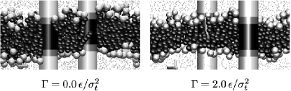
Figure 13: Vertical slices through systems with two inclusions. The dark gray rings above the black hydrophobic part of the protein indicate the sections where the attractive interaction between protein and tail beads (dark gray) decays to zero. The light gray section and the light gray beads mark the hydrophilic part of the protein and the lipid heads, respectively. The solvent beads above and below the bilayer are marked by small dots. The left snapshot shows a stressfree bilayer with proteins of hydrophobically matching length $L=6\,\sigma_{t}$. On the right the same proteins are shown in a bilayer under a tension of $\Gamma=2.0\,\epsilon/\sigma_{t}^{2}$.

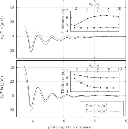
Figure 14: Potential of mean force of two isolated proteins as a function of the protein distance at tension zero (solid lines) and $\Gamma=2.0\,\epsilon/\sigma_{t}^{2}$ (dotted lines), for proteins with hydrophobic length $L=4\,\sigma_{t}$ (top) and $L=6\,\sigma_{t}$ (bottom). The insets show the corresponding radial thickness profiles around a single protein ($d_{p}$ denotes the in-plane distance to the center of the inclusion).

The potentials of mean force between two inclusions as a function of their in-plane distance are plotted in Fig. 14 for two different hydrophobic lengths $L$. In the first case (Fig. 14, top), the inclusion is characterized by a negative hydrophobic mismatch in tensionless free membranes. Under tension, the membrane thins and the mismatch is reduced (inset Fig. 14, top). In the second case (Fig. 14, bottom), the hydrophobic part of the inclusion roughly matches the thickness in the tensionless case. Under tension, the membrane thins and a positive hydrophobic mismatch develops (see inset Fig. 14, bottom).

Due to lipid packing in the vicinity of the inclusions the curves show an oscillatory shape with a wavelength of approximately $1\,\sigma_{t}$. Since at small inclusion-inclusion distances direct interactions of the proteins and depletion induced attraction due to the solvent particles come into play, these parts of the curves have been cut off. Thus, we can focus on the lipid-mediated medium and long ranged interactions. The main effect of tension on the lipid mediated interactions between the two model proteins can be summarized as follows: In the absence of tension, the interactions between hydrophobically mismatched inclusions have an additional attractive contribution, compared to hydrophobically matched inclusions. In the case where the tension reduces the hydrophobic mismatch due to membrane thinning, this attraction diminishes. If, on the other hand, the tension leads to a stronger hydrophobic mismatch, the attractivity of the interaction potential also increases. Therefore, we conclude that the dominant effect of an external tension on the lipid-mediated interactions is indirect and related to the change of the hydrophobic mismatch due to the membrane thinning. For decreasing (negative) mismatch, the average attraction decreases, and for increasing (positive) mismatch, it increases. This is consistent with the behavior observed in tensionless membranes, where also both positive and negative hydrophobic mismatch resulted in an attractive contribution to the PMF West et al. (2009). Other recent studies de Meyer et al. (2008); Schmidt et al. (2008); de Meyer and Smit (2009); Schmidt et al. (2009) have also highlighted the importance of hydrophobic mismatch as a driving factor for protein agglomeration. From our simulations, an additional effect of tension is not evident.

IV Discussion and Summary

In this paper we have studied the influence of an external tension on the properties of bilayers using a generic coarse-grained model. To put these results into perspective, we will now briefly discuss the experimental situation.

Experimentally, one of the most widely used techniques to determine mechanical stretch properties of bilayers is the micropipette approach, where giant bilayer vesicles are pressurized by micropipette suction Kwok and Evans (1981). This method produces a uniform membrane tension, is very accurate, and can be used to verify elastic reversibility Rawicz et al. (2000). Micropipette aspiration experiments, e.g., carried out by Needham and Nun Needham and Nunn (1990), found for different lipids and lipid/cholesterol mixtures that membrane lysis is usually reached at an relative areal expansion of less than $5\,\%$, and the rupture strength at low cholesterol concentration was typically around $2-10\,\textnormal{mN/m}$.

This does not compare well with our findings and those of other atomistic or mesoscopic simulations (see the introduction to Sec. III), where fluid membranes could sustain tensions of $30\,\textnormal{mN/m}$ or more and remained stable up to relative extensions of 40 % or more. It should however be noted that tension-induced lysis is a stochastic process, and the duration of the exposure to the stress plays a decisive role for the stability. Experimentally, abrupt failure of the bilayer is observed, when the tension reaches a critical value, whereas below this tension long-term persistence of the stressed membrane can be presumed Evans and Needham (1987). Evans et al. showed that the rupture strength of membranes is a property which crucially depends on the loading rate Evans et al. (2003). In their study on five types of fluid giant phosphatidylcholine lipid vesicles, they varied the loading rate from $0.01-100\,\textnormal{mN/m/s}$. At high loading rates the systems were found to be stable up to values of $20-30\,\textnormal{mN/m}$.

To get a rough estimate of the meaning of the timescales in our simulations, compared to experimental systems, we can map the diffusion constants $D_{xy}$ in Sec. III.3 to the corresponding values measured for DPPC bilayers in recent experiments. At $45^{\circ}\,\textrm{C}$ Scomparin et al. Scomparin et al. (2009) report a diffusion coefficient of approximately $10\,\mu\textrm{m}^{2}/\textrm{s}$. Taking our result of $D_{xy}=0.8\times 10^{-5}\,\sigma_{t}^{2}/\textrm{MCS}$ for the tensionless membrane and setting our intrinsic length scale $1\,\sigma_{t}$ to $6\,\textrm{\AA}$ as described earlier, we find that $10^{6}\,\textrm{MCS}$ in our simulation correspond to approximately $0.3\,\mu\textrm{s}$ in real time. The typical lengths of our simulations lie between $2$–$4\times 10^{6}\,\textrm{MCS}$, which corresponds to roughly $1\,\mu\textrm{s}$ in real systems. Thus our simulations correspond to systems exposed to very high loading rates and short timescales. Taking this into consideration, their stability does not contradict experimental findings. Our simulations provide a way to study membranes under extreme conditions, and to analyze their structural properties, which cannot be accessed easily by experiments.

Due to these difficulties, experimental results with which we could compare our simulations are scarce. One positive example is the behavior of the the ripple phase under stress. To our knowledge, we have performed the first simulation study which tries to shed light on the structural rearrangements and elastic properties of a bilayer in the ripple phase under lateral stress. We have shown that lateral tension leads to suppression of the ripple structure in the $P_{\beta^{\prime}}$ phase, and we see a transition of the areal extensibility from soft, fluid-like to gel-like behavior. Qualitatively, this behavior agrees well with the findings of Evans et al. Evans and Needham (1987); Needham et al. (1988), who also reported an initial soft-elastic response at low tensions and stiff elastic properties after elimination of the ripple.

In the gel phase, the tension does not change the state of the bilayer significantly in the range of tensions considered in this work. The basic structure of the two monolayers stays intact. The situation is very different in the biologically most relevant fluid phase. At temperatures where the tensionless membranes are fluid, they respond to high tensions by a structural change from a state where both monolayers are well-separated to a state where they are partly interdigitated. These changes are associated with substantial variations of the compressibility (up to a factor of 3), and the lipid diffusion constant (up to 20 %).

We have also studied the influence of membrane tension on the effective interaction between two model proteins. Under tension, the membrane becomes thinner, which affects the hydrophobic mismatch interaction. This is found to be the dominant effect. The interaction between negatively mismatched proteins decreases, and that between positively mismatched proteins increases. Thus applying tension can be used to tune the strength of membrane mediated protein-protein interactions.

References

- Berg et al. (2002) J. M. Berg, J. L. Tymoczko, and L. Stryer, Biochemistry (W. H. Freeman and Company, 2002), 5th ed.
- Nelson et al. (2004) D. Nelson, T. Piran, and S. Weinberg, eds., Statistical Mechanics of Membranes and Surfaces (World Scientific, 2004), 2nd ed.
- Soveral et al. (1997) G. Soveral, R. I. Macey, and T. F. Moura, Biology of the Cell 89, 275 (1997).
- Shillcock and Lipowsky (2005) J. C. Shillcock and R. Lipowsky, Nature Materials 4, 225 (2005).
- Grafmüller et al. (2007) A. Grafmüller, J. Shillock, and R. Lipowsky, Physical Review Letters 98, 218101 (2007).
- Mitragotri (2005) S. Mitragotri, Nature Reviews Drug Discovery 4, 255 (2005).
- Koshiyama et al. (2006) K. Koshiyama, T. Kodama, T. Yano, and S. Fujikawa, Biophysical Journal 91, 2198 (2006).
- Voth (2009) G. A. Voth, ed., Coarse-Graining of Condensed Phase and Biomolecular Systems (CRC Press, 2009).
- Müller et al. (2006) M. Müller, K. Katsov, and M. Schick, Phys. Rep. 434, 113 (2006).
- Deserno (2009) M. Deserno, Macromolecular Rapid Communications 30, 752 (2009).
- Schmid (2009) F. Schmid, Macromolecular Rapid Communications 30, 741 (2009).
- Venturoli et al. (2006) M. Venturoli, M. M. Sperotto, M. Kranenburg, and B. Smit, Physics Reports 437, 1 (2006).
- Lenz and Schmid (2005) O. Lenz and F. Schmid, J. Mol. Liquids 117, 147 (2005).
- Lenz and Schmid (2007) O. Lenz and F. Schmid, Physical Review Letters 98, 058104 (2007).
- West and Schmid (2010, in press) B. West and F. Schmid, Soft Matter (2010, in press).
- West et al. (2009) B. West, F. L. H. Brown, and F. Schmid, Biophysical Journal 96, 101 (2009).
- Tileman et al. (2003) D. P. Tileman, H. Leontiadou, A. E. Mark, and S.-J. Marrink, Journal of the American Chemical Society 125, 6382 (2003).
- Leontiadou et al. (2004) H. Leontiadou, A. E. Mark, and S. J. Marrink, Biophysical Journal 86, 2156 (2004).
- Cooke and Deserno (2005) I. R. Cooke and M. Deserno, Journal of Chemical Physics 123, 224710 (2005).
- Gullingsrud and Schulten (2004) J. Gullingsrud and K. Schulten, Biophysical Journal 86, 2496 (2004).
- Zhu and Vaughn (2005) Q. Zhu and M. W. Vaughn, Journal of Physical Chemistry B 109, 19474 (2005).
- Schmid et al. (2007) F. Schmid, D. Düchs, O. Lenz., and B. West, Computer Physics Communications 177, 168 (2007).
- Mouritsen (2005) O. G. Mouritsen, Life – As a Matter of Fat, The Fontiers Collection (Springer-Verlag, 2005).
- Groot and Rabone (2001) R. D. Groot and K. L. Rabone, Biophysical Journal 81, 725 (2001).
- Grafmüller et al. (2009) A. Grafmüller, J. Shillcock, and R. Lipowsky, Biophysical Journal 96, 2658 (2009).
- Marrink and Mark (2001) S. J. Marrink and A. E. Mark, J. Phys. Chem. 105, 6122 (2001).
- Kranenburg et al. (2003) M. Kranenburg, M. Venturoli, and B. Smit, Physical Review E 67, 060901(R) (2003).
- Irving and Kirkwood (1950) J. H. Irving and J. G. Kirkwood, Journal of Chemical Physics 18, 817 (1950).
- Goetz and Lipowsky (1998) R. Goetz and R. Lipowsky, Journal of Chemical Physics 108, 7397 (1998).
- Brannigan et al. (2006) G. Brannigan, L. C.-L. Lin, and F. L. H. Brown, European Biophysical Journal 35, 104 (2006).
- Gustafsson and Halle (1997) S. Gustafsson and B. Halle, Journal of Chemical Physics 106, 1880 (1997).
- Naji and Brown (2007) A. Naji and F. L. H. Brown, Journal of Chemical Physics 126, 235103 (2007).
- Reister-Gottfried et al. (2007) E. Reister-Gottfried, S. M. Leitenberger, and U. Seifert, Physical Review E 75, 011908 (2007).
- Helfrich (1978) W. Helfrich, Zeitschrift für Naturforschung Section A – A Journal of Physical Science 33, 305 (1978).
- Israelachvili and Wennerström (1992) J. N. Israelachvili and H. Wennerström, Journal of Physical Chemistry 96, 520 (1992).
- Brannigan and Brown (2006) G. Brannigan and F. L. H. Brown, Biophysical Journal 90, 1501 (2006).
- Götz et al. (1999) R. Götz, G. Gompper, and R. Lipowsky, Physical Review Letters 82, 221 (1999).
- Rowlinson and Widom (1982) J. S. Rowlinson and B. Widom, Molecular Theory of Capillarity (Clarendon Press Oxford, 1982).
- Loison et al. (2003) C. Loison, M. Mareschal, K. Kremer, and F. Schmid, Journal of Chemical Physics 119, 13138 (2003).
- Cai et al. (1994) W. Cai, T. C. Lubensky, P. Nelson, and T. Powers., Journal de Physique II 4, 931 (1994).
- Farago and Pincus (2003) O. Farago and P. Pincus, European Physical Journal E 11, 399 (2003).
- Imparato (2006) A. Imparato, Journal of Chemical Physics 124, 154714 (2006).
- Brochard et al. (1976) F. Brochard, P. G. De Gennes, and P. Pfeuty, Journal de Physique 37, 1099 (1976).
- David and Leibler (1991) F. David and S. Leibler, Journal de Physique II 1, 959 (1991).
- Virnau and Müller (2004) P. Virnau and M. Müller, Journal of Chemical Physics 120, 10925 (2004).
- de Meyer et al. (2008) F. J. M. de Meyer, M. Venturoli, and B. Smit, Biophysical Journal 95, 1851 (2008).
- Schmidt et al. (2008) U. Schmidt, G. Guigas, and M. Weiss, Physical Review Letters 101, 128104 (2008).
- de Meyer and Smit (2009) F. J. M. de Meyer and B. Smit, Physical Review Letters 102, 219801 (2009).
- Schmidt et al. (2009) U. Schmidt, G. Guigas, and M. Weiss, Physical Review Letters 102, 219802 (2009).
- Kwok and Evans (1981) R. Kwok and E. Evans, Biophysical Journal 35, 637 (1981).
- Rawicz et al. (2000) W. Rawicz, K. C. Olbrich, T. McIntosh, D. Needham, and E. Evans, Biophysical Journal 79, 328 (2000).
- Needham and Nunn (1990) D. Needham and R. S. Nunn, Biophysical Journal 58, 997 (1990).
- Evans and Needham (1987) E. Evans and D. Needham, Journal of Physical Chemistry 91, 4219 (1987).
- Evans et al. (2003) E. Evans, V. Heinrich, F. Ludwig, and W. Rawicz, Biophysical Journal 85, 2342 (2003).
- Scomparin et al. (2009) C. Scomparin, S. Lecuyer, M. Ferreira, T. Charitat, and B. Tinland, European Physical Journal E 28, 211 (2009).
- Needham et al. (1988) D. Needham, T. J. McIntosh, and E. Evans, Biochemistry 27, 4668 (1988).
- Humphrey et al. (1996) W. Humphrey, A. Dalke, and K. Schulten, Journal of Molecular Graphics 14, 33 (1996).