Many-particle effects in adsorbed magnetic atoms with easy-axis anisotropy: the case of Fe on CuN/Cu(100) surface

Abstract

We study the effects of the exchange interaction between an adsorbed magnetic atom with easy-axis magnetic anisotropy and the conduction-band electrons from the substrate. We model the system using an anisotropic Kondo model and we compute the impurity spectral function which is related to the differential conductance ($dI/dV$) spectra measured using a scanning tunneling microscope. To make contact with the known experimental results for iron atoms on the CuN/Cu(100) surface [Hirjibehedin et al., Science 317, 1199 (2007)], we calculated the spectral functions in the presence of an external magnetic field of varying strength applied along all three spatial directions. It is possible to establish an upper bound on the coupling constant $J$: in the range of the magnetic fields for which the experimental results are currently known (up to $7\,\mathrm{T}$), the low-energy features in the calculated spectra agree well with the measured $dI/dV$ spectra if the exchange coupling constant $J$ is at most half as large as that for cobalt atoms on the same surface. We show that for even higher magnetic field (between 8 and $9\,\mathrm{T}$) applied along the “hollow direction”, the impurity energy states cross, giving rise to a Kondo effect which takes the form of a zero-bias resonance. The coupling strength $J$ could be determined experimentally by performing tunneling spectroscopy in this range of magnetic fields. On the technical side, the paper introduces an approach for calculating the expectation values of global spin operators and all components of the impurity magnetic susceptibility tensor (including the out-of-diagonal ones) in numerical renormalization group (NRG) calculations with no spin symmetry. An appendix contains a density-functional-theory (DFT) study of the Co and Fe adsorbates on CuN/Cu(100) surface: we compare magnetic moments, as well as orbital energies, occupancies, centers, and spreads by calculating the maximally localized Wannier orbitals of the adsorbates.

1 Introduction

Recent advances in the experimental techniques, such as low-temperature scanning tunneling microscopy (STM) and the X-ray magnetic circular dichroism (XMCD), made it possible to study magnetic properties of single adsorbed atoms on various surfaces [1, 2, 3, 4, 5, 6, 7]. Particularly interesting are magnetic impurities on noble metal surfaces where many-particle effects such as the Kondo effect play an important role [8, 9]. Due to the reduced symmetry in the surface region, such magnetic adsorbates are strongly anisotropic [1, 10]. A simple parametrization of the leading magnetic anisotropy terms takes the form of

$$H_{\mathrm{aniso}}=DS_{z}^{2}+E(S_{x}^{2}-S_{y}^{2}),$$ (1)

where the $S_{x}$, $S_{y}$, and $S_{z}$ are the cartesian components of the quantum-mechanical spin-$S$ operator, while the parameters $D$ and $E$ are known as the longitudinal and transverse magnetic anisotropy, respectively. If $D<0$ (the “easy-axis” case), the spin tends to maximize the absolute value of the $z$ component, thus the $S_{z}=\pm S$ states dominate in the ground state doublet, which may be split for integer $S$ even in the absence of an external magnetic field due to the transverse magnetic anisotropy $E$. If $D>0$ (the “easy-plane” or “hard-axis” case), the ground-state is a doublet consisting mostly of the $S_{z}=\pm 1/2$ states for half-integer spin, or a singlet consisting mostly of the $S_{z}=0$ state for integer spin. Similar models are also used to describe molecular magnets [11, 12, 13, 14, 15].

When adsorbed on metallic surfaces, the coupling of the spin to the conduction-band electrons can introduce new phenomena, the Kondo effect being the most interesting due to its unique signature expected in the tunneling spectra. For half-integer spins with easy-plane anisotropy, the level degeneracy in the ground state actually permits the occurrence of the Kondo effect at zero magnetic field, as indeed observed experimentally in the system of cobalt atoms adsorbed on the CuN ultra-thin layers deposited on the Cu(100) substrate surface [16]. For magnetic atoms with easy-axis anisotropy, however, the Kondo effect has not yet been observed. Its absence is either due to the zero-field level splitting caused by the transverse magnetic anisotropy $E$, which in the case of integer $S$ plays the role of an effective magnetic field which suppresses the Kondo effect, or (for half-integer $S$ or for $E\ll|D|$) due to the fact that the spin-flip scattering events of the conduction-band electrons can only change the impurity spin component by 1. Thus the two impurity ground-state levels only couple via higher-order processes and the Kondo screening is strongly suppressed, i.e., the Kondo scale is extremely small [12]. Nevertheless, interesting many-particle effects in fact do occur in the case of easy-axis anisotropy, thus we study this class of the problems in the following parts of the paper, focusing in particular on the case of spin 2 as appropriate for iron atoms adsorbed on the CuN/Cu(100) substrate [10].

The absence of the Kondo effect at zero magnetic field does not imply, that the exchange coupling of an easy-axis magnetic impurity to the substrate is of no consequence. In this work we show that the value of the exchange coupling constant $J$, defined through the Kondo coupling Hamiltonian

$$H_{\mathrm{K}}=J{\boldsymbol{s}}\cdot{\boldsymbol{S}},$$ (2)

where ${\boldsymbol{s}}$ is the spin-density of the conduction-band electrons at the position of the impurity, affects the impurity spectral function in a measurable way. The most drastic effect is the occurrence of a Kondo effect induced by a magnetic field, similar to the singlet-triplet Kondo effect in quantum dot systems [17, 18, 19, 20, 21, 19, 22]: for some high enough external magnetic field applied along the $x$-axis, the impurity level crossing leads to a situation where the conditions for the occurrence of a Kondo effect are met. We will show that the presently available experimental results (measured up to $7\,\mathrm{T}$, Ref. [10]) just stop short of the region where this Kondo resonance should be observed (between $8\,\mathrm{T}$ and $9\,\mathrm{T}$). For this reason, the presently known experimental results can only be used to establish an upper bound on the value of $J$, but by extending the magnetic field range into the $9\,\mathrm{T}$ range, the Kondo resonance could be probed and the exchange coupling $J$ might be determined even quantitatively.

The paper is structured as follows. In Sec. 2 we provide the full definition of the model under study and describe the numerical technique which is used to compute the impurity spectral function. We also comment on the relation between the impurity spectral function and the experimentally measured $dI/dV$ spectrum. In Sec. 3 we discuss the impurity level structure and the predicted $dI/dV$ spectra in the limit of a decoupled impurity, $J\to 0$. Such spectra do not encompass any many-particle effects; however, they account accurately for the high-energy spin excitations which are observed experimentally. In Sec. 4 the results of the numerical calculations for the full many-particle problem are presented and discussed in relation with the experimental results. A presents a comparative density-functional-theory (DFT) study of Co and Fe adatoms on the CuN/Cu(100) surface, while B contains the description of a method for computing the thermodynamic impurity spin susceptibility in problems having no symmetries in the spin space with the numerical renormalization group (NRG) method.

2 Model and method

We model the system using the Hamiltonian $H=H_{\mathrm{band}}+H_{\mathrm{K}}+H_{\mathrm{imp}}$ where

$$H_{\mathrm{band}} =\sum_{k\sigma}\epsilon_{k}c^{\dagger}_{k\sigma}c_{k\sigma},$$ (3)

$$H_{\mathrm{imp}} =g\mu_{B}{\boldsymbol{B}}\cdot{\boldsymbol{S}}+H_{\mathrm{aniso}}.$$ (4)

The anisotropy term $H_{\mathrm{aniso}}$ is given by Eq. (1), and the coupling term $H_{\mathrm{K}}$ by Eq. (2). The operator $c_{k\sigma}$ corresponds to a conduction-band electron with momentum $k$, spin $\sigma\in\{\uparrow,\downarrow\}$, and energy $\epsilon_{k}$. In terms of these operators, the spin density of the conduction-band electrons at the position of the impurity (assumed to be at the origin of the coordinate system) is given by ${\boldsymbol{s}}=(1/2)f^{\dagger}_{0,\alpha}\boldsymbol{\sigma}_{\alpha\beta}f_{0,\beta}$, where

$$f_{0\sigma}=\frac{1}{\sqrt{N}}\sum_{k}c_{k\sigma},$$ (5)

$N$ is the number of the conduction-band states, and $\boldsymbol{\sigma}_{\alpha\beta}$ is the vector of Pauli matrices. Finally, $g$ is the gyromagnetic factor (assumed to be isotropic), and $\mu_{B}\approx 0.0579\mathrm{meV/T}$ is the Bohr magneton. For an iron adatom on the CuN/Cu(100) surface, the following parameters have been established: spin $S=2$, $g=2.11\pm 0.05$, $D=-1.55\pm 0.01\,\mathrm{meV}$, $E=0.31\pm 0.01\,\mathrm{meV}$ (Ref. [10]). For a complete description one should, furthermore, know the density of states (DOS) of the conduction band, $\rho(\omega)=(1/N)\sum\delta(\omega-\epsilon_{k})$, and the value of the Kondo coupling $J$. In the interesting energy range (on the order of $10\,\mathrm{meV}$ around the Fermi level) the energy dependence of the DOS may be neglected and we can use a constant value $\rho=\rho(\omega=0)$. The low-energy behavior of the problem then depends solely on the dimensionless combination $\rho J$. We note that the model does not include any orbital moment degrees of freedom. This approximation is based on the fact that the orbital moment of an impurity adsorbed on the surface is typically strongly quenched due to the surface field effects (for the particular case of Fe and Co adsorbates on the surface of CuN/Cu(100), the total suppression of orbital degeneracy follows from the DFT results tabulated in A).

We solve the problem using the numerical renormalization group [23, 24, 25] (for the details on the application of the NRG to the problems of this class see also Refs. [26, 27]). In this work, the focus of our interest will be the impurity spectral function defined as [28]

$$A_{\sigma}(\omega)=-\frac{1}{\pi}\mathrm{Im}T_{\sigma}(\omega+i\delta),$$ (6)

where $T_{\sigma}(\omega)$ is the T-matrix for the scattering of electrons of spin $\sigma$ on the spin-$S$ impurity, given by

$$T_{\sigma}(\omega)=\frac{J}{2}\langle S_{z}\rangle+\langle\langle O_{\sigma};O_{\sigma}^{\dagger}\rangle\rangle_{\omega},$$ (7)

with the operators

$$O_{\uparrow} =\frac{J}{2}\left(f_{0\downarrow}S^{-}+f_{0\uparrow}S_{z}\right),$$ (8)

$$O_{\downarrow} =\frac{J}{2}\left(f_{0\uparrow}S^{+}-f_{0\downarrow}S_{z}\right).$$ (9)

Here $S^{\pm}=S_{x}\pm iS_{y}$. The notation $\langle\langle A;B\rangle\rangle_{\omega}$ denotes the Laplace transform of the correlator $\langle\langle A;B\rangle\rangle_{t}=-i\theta(t)\langle\{A(t),B(0)\}_{+}\rangle$ between two (fermionic) operators $A$ and $B$, i.e., $\langle\langle A;B\rangle\rangle_{\omega}=\int_{0}^{\infty}e^{i\omega t}\langle\langle A;B\rangle\rangle_{t}\mathrm{d}t$ with $\mathrm{Im}\,\omega>0$; $\{A,B\}_{+}=AB+BA$ is the anti-commutator.

The T-matrix itself is defined through

$$G_{kk^{\prime}\sigma}(\omega)=\delta_{kk^{\prime}}G_{kk^{\prime}\sigma}^{0}(\omega)+G^{0}_{kk\sigma}(\omega)\frac{1}{N}T_{\sigma}(\omega)G^{0}_{k^{\prime}k^{\prime}\sigma}(\omega),$$ (10)

where $G_{kk\sigma}(\omega)=\langle\langle c_{k\sigma};c_{k\sigma}^{\dagger}\rangle\rangle$ is the conduction-band electron Green’s function and $G^{0}_{kk\sigma}$ its unperturbed counterpart. In the STM experiments, the spin components are not resolved, thus we will mostly plot the spin-averaged spectral functions, $A(\omega)=[A_{\uparrow}(\omega)+A_{\downarrow}(\omega)]/2$.

3 Decoupled impurity limit

The spin excitation spectrum of a magnetic atom adsorbed on a thin insulating layer may for the most part be accounted for by fully neglecting its exchange coupling to the substrate electrons. According to this picture, the tunneling differential conductance will increase stepwise when the bias voltage is increased beyond the values $(E_{i}-E_{gs})/e$, where $E_{i}$ are the energies of the excited states and $E_{gs}$ is the ground-state energy [2, 3, 10]. At each of these voltages, an additional inelastic scattering (spin-flip) channel opens, typically resulting in an increased conductance [29, 30, 31, 32, 33, 34, 35, 36, 37]. In fact, the experiments have shown that the conductance step heights are described to a good approximation by [2]

$$|\langle i|S_{x}|gs\rangle|^{2}+|\langle i|S_{y}|gs\rangle|^{2}+|\langle i|S_{z}|gs\rangle|^{2},$$ (11)

i.e., by the transition matrix elements for the spin operator. This empirical observation has recently received theoretical support [38, 39]. The expression suggests that the impurity is well thermalized with the substrate: the impurity relaxes to the ground-state on a time-scale which is short compared with the mean time between the tunneling events. Using this simple approach, one can compute $dI/dV$ spectra which compare very well with the experimental results (as long as the many-particle effects are not important) if thermal broadening is taken into account. Here we show the results obtained by this procedure without adding any artificial thermal smearing, see Fig. 1a. The plots should be compared with Fig. 2A,B,F and Fig. S1,A,C in Ref. [10]. Presenting the results in the zero-temperature limit uncovers more details, in particular the crossing of the the levels in the case of a field applied along the $x$-axis (this corresponds to the “hollow axis” in Ref. [10]).

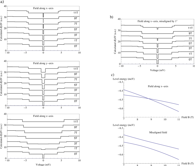
Figure 1: a) Simulated IETS spectra. No thermal broadening has been applied. b) Simulated IETS spectra for a field with a direction almost along the $x$-axis with a small component along the $z$-axis (misalignment by $1\,\mathrm{{}^{\circ}}$. c) Energy-level diagrams for a field along the $x$-axis (top) and for a field misaligned by $1\,\mathrm{{}^{\circ}}$ (bottom).

As is well known, the experimental results are in very good agreement with the simulated $dI/dV$ spectra [10]. One comment, however, is in order. In experiments, the step height of the first step in the dI/dV spectra is observed to decrease as the field strength along the $x$-axis is increased. This can be explained, on one hand, by the thermal broadening of the spectra which leads to reduced heights of spectral features of the width smaller than the width of the broadening kernel. Another explanation is based on a possibility of a slight misalignment of the magnetic field from the direction of the actual $x$-axis of the magnetic atom. A simple calculation (Fig. 1b) shows that even a small misalignment of $1\,\mathrm{{}^{\circ}}$ (which is quite likely to occur) can suppress the step height of the first excitation (at $T=0$) without significantly modifying those at the other magnetic excitation energies.

We now comment on the important observation that the energy difference between the two lowest levels decreases as the field strength along the $x$-axis is increased, see Fig. 1c, top. A simple calculation neglecting any possible many-particle effects indicates that the levels become degenerate at

$$B_{x}=\frac{1}{g\mu_{B}}\sqrt{2E(E-D)}\approx 8.8\,\mathrm{T}.$$ (12)

For this field strength, a magnetic-field-induced Kondo effect can occur if the Kondo exchange coupling is antiferromagnetic, $J>0$. We note that the aforementioned misalignment of the field will also tend to suppress the Kondo effect at $B_{x}\approx 8.8\,\mathrm{T}$, since a component of the field along the $z$-axis will mix the levels, thereby leading to an avoided crossing of the levels (Fig. 1c, bottom). In experiments seeking to detect the field-induced Kondo effect, it will be thus essential to not only fine-tune the magnitude of the magnetic field, but also its exact direction.

4 Impurity spectral functions

In Fig. 2 we plot the impurity spectral functions $A(\omega)$ computed using the numerical renormalization group (NRG). The calculation is performed for zero temperature, thus the widths of spectral features are due to intrinsic effects (the NRG spectral function overbroadening artifacts are small in these calculations; for discussion see Ref. [40]). Compared with the simulated $dI/dV$ curves, all spectral features except for those near the Fermi level are almost completely smeared out. This is at odds with the experimental results, where the steps are observed to be sharp apart from the thermal broadening. While the calculated spectral function does encompass some inelastic scattering effects (see Fig. 3 in Ref. [27]), the tunneling current includes additional inelastic scattering contributions which are beyond the scope of our calculations that are constrained to the case of the magnetic impurity being in thermal equilibrium with the substrate electron reservoir at all times and do not include any additional interactions between the tunneling electron and the impurity local moment. Nevertheless, the results obtained from a NRG calculation provide a reliable description of the behavior of the system in the immediate vicinity of the Fermi level, which is probed by tunneling electrons of sufficiently low-energy so that the system is not driven significantly out of the equilibrium.

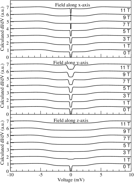
Figure 2: Impurity spectral functions $A(\omega)$ computed using the NRG. The horizontal energy axis has been transformed to show the equivalent bias voltages, while the vertical axis corresponds to the $dI/dV$ differential conductance in the simple approximation where the LDOS is taken to be proportional to the spectral function. Here $\rho J=0.05$.

The agreement between the low-energy features (interval $[-1\,\mathrm{mV}:+1\,\mathrm{mV}]$) in the calculated and measured spectra [10] in the 0 to 7 T range is very good if thermal broadening is taken into account. The calculation was performed for $\rho J=0.05$. This value is half as large as the exchange coupling for Co impurities on the same surface, $\rho J=0.1$, which has been established in Refs. [26, 27]) by determining the value of $\rho J$ that allows to reproduce the experimental differential conductance spectra for the Co/CuN/Cu(100) adsorbate system. Due to similarities between Co and Fe atoms the exchange coupling constants should not be too different, but very likely of the same order of the magnitude and of the same sign (Co and Fe are neighbours in the periodic system; see A for a more rigorous comparative study using the density functional theory). In Fig. 3a we compare the low-energy part of the spectral function for a fixed magnetic field of 7 T in the $x$-axis direction for a range of values of $J$. For large $J$, the dip in the spectral density turns into a (Kondo) resonance which becomes fully developed for $\rho J\geq 0.1$. For $\rho J$ in the interval 0.06 to 0.1, we find an intermediate structure: a dip with protrusions at the step edges. At high enough temperature, the protrusions will be washed out and a single antiresonance would be detected. Taking all these elements into account, the estimate of the upper bound $\rho J=0.05\pm 0.02$ therefore seems reasonable.

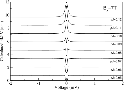
Figure 3: Impurity spectral functions for $7\,\mathrm{T}$ magnetic field applied along the $x$-axis for a range of $\rho J$.

The magnetic field at which the Kondo effect occurs for integer spin Fe is not given exactly by Eq. (12), but it rather depends on the value of $J$, since the different impurity levels are renormalized differently due to the anisotropy. In the $J\to 0$ limit, the Kondo effect occurs at $B_{x}\approx 8.8\,\mathrm{T}$, while for finite $J$ the magnetic field where the Kondo peak may be observed is reduced. In addition, the parameter $J$ controls the width of the Kondo resonance (and, of course, the Kondo temperature itself), thus for smaller $J$ the interval of the magnetic fields where the Kondo effect may be observed is accordingly narrower and the Kondo scale lower.

The magnetic-field-induced Kondo effect exhibits a number of rather peculiar features. We first note that it is very difficult to observe the fully developed Kondo resonance unless $J$ is rather large. For the estimated exchange coupling of $\rho J=0.05$, where the Kondo effect occurs for $B_{x}^{*}=8.535\,\mathrm{T}$, the Kondo temperature is actually extremely low, on the order of $0.1\,\mathrm{mK}$, see Fig. 4. Even at dilution refrigerator temperatures, it thus appears unlikely that a fully developed Kondo resonance will be observed. This does not, however, preclude the experimental detection of the Kondo physics at play in this system, since the evolution of the tunneling spectrum as the magnetic field is tuned should exhibit a characteristic merging of the two “half-resonances”.

The results for the thermodynamic properties also reveal that the $zz$ component of the magnetic susceptibility multiplied by the temperature [i.e., the effective moment $T\chi_{zz}(T)$] exhibits a plateau at very high value of 3.5 (in suitable units), which is rather near the limiting value for a decoupled $S_{z}=\pm 2$ doublet, which is 4. This plateau corresponds to a $\ln 2$ plateau in the impurity entropy, i.e., to an effective two-state system. On the scale of $T_{K}$, the moment is then screened. Note that the temperature dependence of $T\chi_{zz}(T)$ is different (Kondo-like, see the arrow in Fig. 4) for $B_{x}=B_{x}^{*}$ as compared with those for other values of the magnetic field, which merely follow the $\exp(-\Delta E/k_{B}T)$ rule, where $\Delta E$ is the difference between the two lowest impurity level energies.

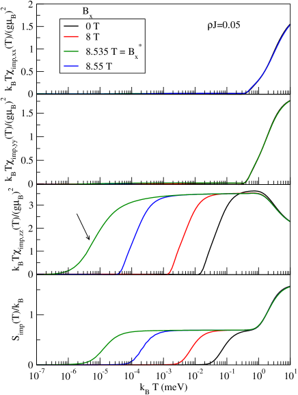
Figure 4: Thermodynamic properties for a range of magnetic fields along the $x$-axis. We plot the impurity contribution to the magnetic susceptibility in various directions, $\chi_{\mathrm{imp},\alpha\alpha}$, where $\alpha\in\{x,y,z\}$ is a direction in space, and the impurity contribution to the entropy, $S_{\mathrm{imp}}$. The Kondo temperature is estimated from the data for $S_{\mathrm{imp}}$ to be $T_{K}\sim 10^{-5}\,\mathrm{meV}\sim 0.1\,\mathrm{mK}$. The arrow points to the curve with exhibits Kondo-like temperature dependence.

It is equally interesting to note that the spectral functions change discontinuously as we cross the transition value $B_{x}^{*}$, see Fig. 5a; this corresponds to the system being in different ground states on either side of the transition. In the presence of a small magnetic field component along the $z$-axis, the level-crossing is replaced by a rapid cross-over. Any such rapid change of the spectral function over an extended energy interval would be an indicator of the proximity to the Kondo regime, even at higher temperatures.

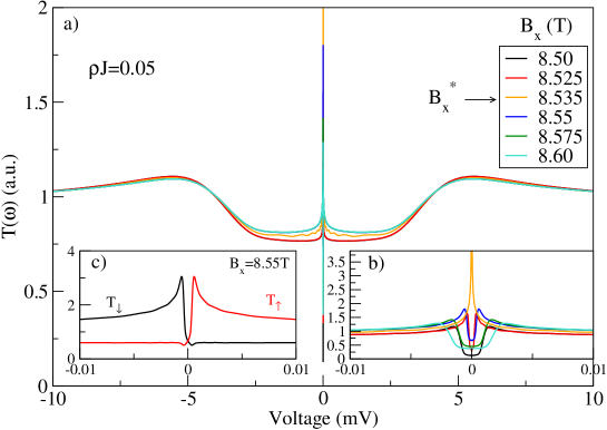
Figure 5: Impurity spectral functions in the vicinity of the magnetic-field-induced Kondo effect at $B_{x}=B_{x}^{*}$. a) Overview plot, b) close-up on the low-voltage region. The jaggedness of the curve at the transition point is due to increased numeric artifacts related to the ground-state crossing. c) Spin-resolved spectral function away from the transition point. Note the rather sharp features in the field-split Kondo resonance.

The magnetic-field-induced Kondo effect is not the only observable consequence of the exchange coupling with the substrate. The value (as well as the sign) of $J$ is actually reflected in the spectral function for any value of the magnetic field. In Fig. 6 we compare, for example, the impurity spectral function at zero field for a range of coupling constants. The exchange coupling strongly affects the features around the Fermi level, but also those at higher energies, although to a lesser degree.

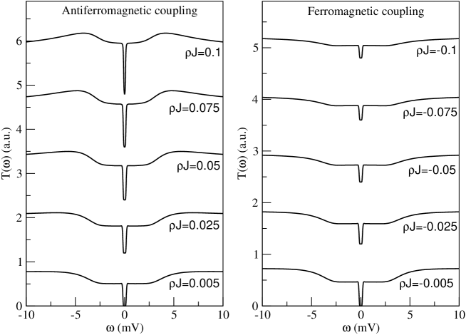
Figure 6: Impurity spectral functions at zero field for different values of exchange coupling $J$.

The results which we have established for the $S=2$ Kondo model also apply more generally for other integer spins: at some $B_{x}^{*}$ there will be level crossing which can induce a Kondo resonance at the Fermi level, but no such crossing occurs for the magnetic field along the $y$ and $z$ axis. The same is true for half-integer spin models, but in this case there is, in addition, a two-fold level degeneracy also for zero magnetic field, thus for half-integer-spin magnetic impurities one could observe both the zero-field Kondo effect and the magnetic-field-induced Kondo effect.

5 Conclusion

We have studied thermodynamic and spectral properties of the Kondo model with an easy-axis anisotropy. By comparing the calculated spectral functions with the measured ones in the magnetic field range up to $7\,\mathrm{T}$ we have estimated the upper bound for the exchange coupling of a Fe adatom on CuN/Cu(100) surface with the bulk conduction-band electrons to be $\rho J=0.05\pm 0.02$. By extending the range of the magnetic fields in the experiments up to $9\,\mathrm{T}$, it should be possible to obtain an improved upper bound on $J$ or perhaps even observe a magnetic-field-induced Kondo resonance if $J$ is high enough. We note here that, strictly speaking, the quantity $J$ scales under the renormalization-group flow, thus its actual value depends on the choice of the bandwidth and the corresponding density of states $\rho$; a more rigorous treatment of the problem would take into account the full density-of-states dependence of the substrate and, furthermore, the momentum dependence of the Kondo coupling $J({\boldsymbol{k}},{\boldsymbol{k}}^{\prime})$, see for example Ref [41]. Nevertheless, a simple characterization in terms of the dimensionless combination $\rho J$ is sufficient to compare the over-all effect of the Kondo screening for different adsorbed atoms.

For quantitative estimates, it will be important also to reduce the temperature at which the experiments are performed as far as possible. Irrespective if the Kondo resonance around $8.5\,\mathrm{T}$ will eventually be observed or not, the real motivation for performing such experiments actually comes from the need to estimate the exchange coupling to the bulk electrons, since this parameter also determines the spin relaxation time; thus it plays an important role in the possible applications of high-spin states of magnetic impurities for storing and processing information.

Appendix A DFT study of Co and Fe adatoms on CuN/Cu(100)

Table 1: Properties of the Co and Fe adatom on CuN/Cu(100) surface.

• System	Moment ($\mu_{B}$/cell)	$n_{d}$	$n_{d\uparrow}-n_{d\downarrow}$	$n_{s}$
  Co/Cu2N/Cu(100)	2.88	7.56	2.10	0.64
  Fe/Cu2N/Cu(100)	4.12	6.61	3.09	0.63

Table 2: The properties of the MLWFs of Co on CuN/Cu(100). We tabulate orbital energy $\epsilon$, occupancy $n$, orbital spread $s$, and orbital center along the $z$-axis. The orbital labels correspond to the initial projections used in the calculation of the corresponding maximally localized Wannier orbitals, although the orbitals are significantly modified from the free-atom orbitals due to the strong hybridization with the neighboring N atoms and the Cu atom just below the adsorbate. The position of the Co adatom in the $z$-direction is $z(\mathrm{Co})=$-0.148 Å; the origin for the $z$-axis corresponds to the top-most layer of Cu atoms prior to relaxation.

• Co	Minority spin $\downarrow$				Majority spin $\uparrow$
  Orbital	$\epsilon$ (eV)	$n$	$s$ (Å2)	$z$ (Å)	$\epsilon$ (eV)	$n$	$s$ (Å2)	$z$ (Å)
  $s$	01.70	0.27	2.36	-3.06	01.32	0.37	2.07	-3.03
  $d_{3z^{2}-r^{2}}$	-1.01	0.88	0.73	-2.01	-2.41	0.97	0.52	-2.06
  $d_{zx}$	-0.07	0.28	0.94	-2.09	-2.83	1.00	0.42	-2.15
  $d_{zy}$	-0.50	0.41	0.50	-2.17	-2.98	0.97	0.44	-2.17
  $d_{x^{2}-y^{2}}$	-1.04	0.80	1.16	-2.03	-2.30	0.90	0.77	-2.08
  $d_{xy}$	-0.34	0.36	0.65	-2.12	-2.90	0.99	0.46	-2.13
  $d$ total		2.73				4.83

Table 3: The properties of the MLWFs of Fe on CuN/Cu(100). The position of the Fe adatom in the $z$-direction is $z(\mathrm{Fe})=$-0.158 Å.

• Fe	Minority spin $\downarrow$				Majority spin $\uparrow$
  Orbital	$\epsilon$ (eV)	$n$	$s$ (Å2)	$z$ (Å)	$\epsilon$ (eV)	$n$	$s$ (Å2)	$z$ (Å)
  $s$	01.59	0.22	2.34	-3.13	00.50	0.41	2.02	-3.16
  $d_{3z^{2}-r^{2}}$	-0.31	0.49	0.76	-2.18	-3.26	0.97	0.47	-2.23
  $d_{zx}$	00.63	0.10	0.98	-2.12	-3.56	1.00	0.43	-2.30
  $d_{zy}$	00.22	0.26	0.50	-2.35	-3.33	0.99	0.51	-2.33
  $d_{x^{2}-y^{2}}$	-0.30	0.72	1.29	-2.17	-2.65	0.90	0.70	-2.23
  $d_{xy}$	00.52	0.19	0.47	-2.27	-3.19	0.99	0.47	-2.27
  $d$ total		1.76				4.85

To further substantiate our claim of the similarities between Co and Fe, which are neighbours in the periodic system differing by a single electron, we have performed a detailed comparative study using the density functional theory (DFT) [42, 43]. We used the PWSCF code (from the Quantum Espresso package, http://www.quantum-espresso.org/, Ref. [44]) with a plane-wave basis set, ultra-soft pseudopotentials, and Perdew-Burke-Ernzerhof $\sigma$-GGA exchange-correlation functional [45, 46, 44]. The kinetic-energy cutoff was 35 Ry and the density cut-off 400 Ry. We used an 8x8x4 Monkhorst-Pack mesh of $k$-points in the self-consistent-field band-structure calculation (but 6x6x1 for the initial relaxation calculation). The cold-smearing by 0.035 Ry has been performed using the Marzari-Vanderbilt scheme [47]. We used the experimentally-determined lattice constant for Cu, $a=0.361\,\mathrm{nm}$. The substrate was modeled using a 2-by-2 supercell in the lateral direction consisting of 4 Cu layers (i.e., 37 atoms in total including the N atoms and the adsorbate). The Cu atoms in the bottom-most layer were fixed, while all others were allowed to relax. We note that similar calculations have already been performed for Fe and Mn adatoms [10] and recently also for Mn chains [48] on the same surface.

To gain more insight into the orbital structure of the impurities, we have also calculated the maximally localized Wannier functions (MLWF) [49, 50] on the impurity site using the Wannier90 package (http://www.wannier.org/, Ref. [51]). The MLWFs provide a very compact and accurate local representation of the electronic structure: they give direct insight into the nature of the chemical bonding. A 4x4x2 uniform grid of $k$-points was used here. The initial projections consisted of $d$ and $s$ states on the adatom and the Cu atoms, and of $sp3$ hybridized states on the N atom; in addition, $s$ states were added in the interstitial sites of the lattice to describe the delocalized electrons (1 per Cu atom). The energy window was chosen so as to encompass all $d$ and $s$ levels of the adatom.

Table 1 presents an overview of the results: the magnetic moment and the occupancies of the adatom levels. The results are expected – the two adatoms differ by one electron in the $d$ orbital. More details can be found in Tables 2 and 3 where we show the orbital energies (defined as the average energy of the spectral function of a particular MLWF), occupancies (defined as the integral of the spectral function of MLWF up to the Fermi energy), the centers of the MLWFs, as well as their spreads. It is manifest that the difference consists of one additional electron in the “minority” spin orbitals for the Co adatom. In fact, the spectral functions shown in Fig. 7 reveal that the “majority” spin spectral functions are essentially the same in both cases, while the “minority” spin spectral functions are to a good approximation just rigidly shifted.

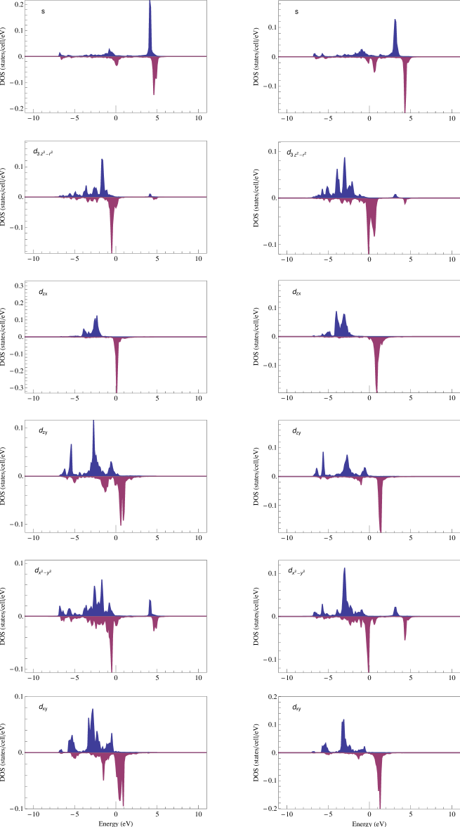
Figure 7: Partial density of states (spectral functions) for the MLWF on Co (left) and Fe (right) adatoms. We plot both spin projections: “majority” spin (above), “minority” spin (below). The spectral functions were computed on a 16x16x3 grid of $k$-points with a 0.1 eV binning resolution.

Appendix B Calculation of the magnetic susceptibility in anisotropic models

In general, the magnetic susceptibility is calculated as [52, 25]:

$$\chi_{\alpha}(T)=(g\mu_{B})^{2}\int_{0}^{\beta}d\tau\left(\langle S_{\alpha}(\tau)S_{\alpha}(0)\rangle-\langle S_{\alpha}\rangle^{2}\right),$$ (13)

where $S_{\alpha}$ is the $\alpha\in\{x,y,z\}$ component of the spin and $\beta=1/k_{B}T$. The impurity contribution to the total magnetic susceptibility, $\chi_{\mathrm{imp},\alpha}$, is then obtained by subtracting the susceptibility of a system without the impurity, $\chi^{(0)}_{\alpha}(T)$, from the magnetic susceptibility of the full system (i.e., the continuum of the conductance-band electrons plus the impurity), $\chi_{\mathrm{full},\alpha}(T)$:

$$\chi_{\mathrm{imp},\alpha}(T)=\chi_{\mathrm{full},\alpha}(T)-\chi^{(0)}_{\alpha}(T).$$ (14)

In the problems with $\mathrm{U}(1)$ spin symmetry, $S_{z}$ is a conserved quantum number and it is used to classify the invariant subspaces of the Hilbert space, thus the calculation of the expectation values in (13) is particularly simple for $\alpha=z$:

$$\chi_{z}(T)=(g\mu_{B})^{2}\beta\left(\langle S_{z}^{2}\rangle(T)-\left[\langle S_{z}\rangle(T)\right]^{2}\right),$$ (15)

where $\langle S_{z}\rangle(T)=(1/Z^{(N)})\sum_{S_{z},n}S_{z}\exp(-\beta E^{(N)}_{S_{z};n})$ and similarly for $\langle S_{z}^{2}\rangle(T)$. Here $Z^{(N)}$ is the partition function at shell $N$, defined as $Z^{(N)}=\Tr_{N}(e^{-\beta H})=\sum_{S_{z},n}\exp(-\beta E^{(N)}_{S_{z};n})$, $S_{z}$ the conserved spin quantum number, $n$ a multi-index composed of all the remaining quantum numbers used to classify the states, and $E^{(N)}_{S_{z};n}$ the energy of the state with given quantum numbers. For other directions $\alpha$, and for more general problems without any symmetry in the spin space, a full dynamical calculation of the correlator $\langle S_{\alpha}(\tau)S_{\alpha}(0)\rangle$ has to be performed.

The calculation of $\chi_{\alpha}$ requires an iteration of the operator matrix elements for all components of the total spin operator $S_{\alpha}$. The approach is similar to the calculation of the matrix elements of an arbitrary local impurity operator, but it is extended to allow for total (“global”) spin operators $S_{\alpha}$. The matrix elements at a given step $N+1$ are calculated from those at the previous step by using the unitary basis transformation resulting from the diagonalization of the Hamiltonian matrices. We follow the notation of Ref. [25]; see Eqs. (39,40,43) in the cited work:

$$|w\rangle_{N+1}=\sum_{rs}U(w,rs)|r;s\rangle_{N+1},$$ (16)

with

$$|r;s\rangle_{N+1}=|r\rangle_{N}\otimes|s(N+1)\rangle.$$ (17)

Here $r$ indexes the eigenpairs of the chain Hamiltonian at the previous iteration, i.e., $H_{N}|r\rangle_{N}=E_{N}(r)|r\rangle_{N}$, the states $|s(N+1)\rangle$ constitute a basis for the added site, while $U(w,rs)$ is the unitary matrix which diagonalizes the Hamiltonian $H_{N+1}$, so that $H_{N+1}|w\rangle_{N+1}=E_{N+1}|w\rangle_{N+1}$. We write $\hat{{\boldsymbol{S}}}_{\alpha}^{N+1}=\hat{{\boldsymbol{S}}}_{\alpha}^{N}+\hat{{\boldsymbol{s}}}_{\alpha}^{N+1}$, where $\hat{{\boldsymbol{S}}}^{N}$ is the total spin operator up to (and including) the site $N$, while $\hat{{\boldsymbol{s}}}^{N+1}$ denotes the local spin operator on site $N+1$. The matrix elements are then updated as follows [compare with (75) in Ref. [25]]:

$$M^{N+1}_{ww^{\prime}} ={}_{N+1}\langle w|\hat{S}_{\alpha}^{N+1}|w^{\prime}\rangle_{N+1}$$ (18)

$$=\sum_{rs}U(w,rs){}_{N+1}\langle r;s|\hat{S}_{\alpha}^{N+1}\cdot\sum_{r^{\prime}s^{\prime}}U(w^{\prime},r^{\prime}s^{\prime})|r^{\prime};s^{\prime}\rangle_{N+1}$$ (19)

$$=\sum_{rs,r^{\prime}s^{\prime}}U(w,rs)U(w^{\prime},r^{\prime}s^{\prime})\Bigl{(}{}_{N}\langle r|\hat{S}_{\alpha}^{N}|r\rangle_{N}\delta_{ss^{\prime}}$$ (20)

$$\quad\quad+\delta_{rr^{\prime}}\langle s|\hat{s}_{\alpha}^{N+1}|s^{\prime}\rangle\Bigr{)}$$ (21)

$$=\sum_{s}\sum_{rr^{\prime}}U(w,rs)M^{N,s}_{rr^{\prime}}U(w,r^{\prime}s)$$ (22)

$$\quad\quad+\sum_{ss^{\prime}}\left(\sum_{r}U(w,rs)U(w^{\prime},rs^{\prime})\right)\langle s|\hat{s}_{\alpha}|s^{\prime}\rangle.$$ (23)

The first part of the expression on the right-hand side, (22), is exactly the same as the conventional prescription for the recursive calculation of the matrix elements of the operators which are singlets with respect to the symmetry group of the Hamiltonian: for each contribution $s$, one performs a similarity transformation of the matrix $M^{N,s}$ from the previous iteration. The second part of the expression, (23), consists in adding the matrix elements of the spin operator for the additional site weighted by the inner-products between the columns of submatrices of the unitary transformation $U$.

At each iteration, the required expectation values are calculated in the same way as for local singlet operators [cf. (58) in Ref. [25]]:

$$\langle S_{\alpha}\rangle(T_{N})\approx\frac{1}{Z^{(N)}}\sum_{w}M^{N}_{ww}$$ (24)

where the matrix elements $M^{N}_{ww}$ are those that correspond to the operator $S_{\alpha}$.

The imaginary-time integral of the correlator $C(\tau)=\langle S_{\alpha}(\tau)S_{\alpha}(0)\rangle$ may be expressed using the Lehmann representation as

$$\int_{0}^{\beta}C(\tau)\mathrm{d}\tau=\frac{1}{Z^{(N)}}\sum_{w,w^{\prime}}\left(M^{N}_{ww^{\prime}}\right)^{*}M_{w^{\prime}w}^{N}\frac{e^{-\beta E_{w}}-e^{-\beta E_{w^{\prime}}}}{\beta E_{w^{\prime}}-\beta E_{w}}.$$ (25)

Note that for the spin operator along the $y$ direction, the NRG calculation has to be performed using complex numbers.

Where comparisons can be made (e.g., in isotropic models) the magnetic susceptibility calculated in the traditional way and using the proposed technique differ by no more than a few per mil in calculations performed for $\Lambda=2$, and even less for higher $\Lambda$. We observed, however, that more states need to be kept in this approach than in the standard NRG thermodynamic calculations. The calculation of $\chi$ is made possible by the property of the energy-scale separation of total spin operators, much like the entire NRG iteration is based on the energy-scale separation property of the Hamiltonian.

The approach described in this section can be immediately generalized to the calculation of the out-of-diagonal components of the magnetic susceptibility tensor.

References

- [1] P. Gambardella, S. Rusponi, M. Veronese, S. S. Dhesi, C. Grazioli, A. Dallmeyer, I. Cabria, R. Zeller, P. H. Dederichs, K. Kern, C. Carbone, and H. Brune. Giant magnetic anisotropy of single cobalt atoms and nanoparticles. Science, 300:1130, 2003.
- [2] A. J. Heinrich, J. A. Gupta, C. P. Lutz, and D. M. Eigler. Single-atom spin-flip spectroscopy. Science, 306:466, 2004.
- [3] Cyrus F. Hirjibehedin, Christopher P. Lutz, and Andreas J. Heinrich. Spin coupling in engineered atomic structures. Science, 312:1021, 2006.
- [4] F. Meier, L. H. Zhou, J. Wiebe, and R. Wiesendanger. Revealing magnetic interactions from single-atom magnetization curves. Science, 320:82, 2008.
- [5] T. Balashov, T. Schuh, A. F. Takacs, A. Ernst, S. Ostanin, J. Henk, I. Mertig, P. Bruno, T. Miyamachi, S. Suga, and W. Wulfhekel. Magnetic anisotropy and magnetization dynamics of individual atoms and clusters of fe and co on pt(111). Phys. Rev. Lett., 102:257203, 2009.
- [6] M. Ternes, A. J. Heinrich, and W. D. Schneider. Spectroscopic manifestations of the kondo effect on single adatoms. J. Phys.: Condens. Matter, 21:053001, 2009.
- [7] H. Brune and P. Gambardella. Magnetism of individual atoms adsorbed on surfaces. Surf. Sci., 602:1812, 2009.
- [8] J. Li, W.-D. Schneider, R. Berndt, and B. Delley. Kondo scattering observed at a single magnetic impurity. Phys. Rev. Lett., 80:2893, 1998.
- [9] V. Madhavan, W. Chen, T. Jamneala, M. Crommie, and N. S. Wingreen. Tunneling into a single magnetic atom: Spectroscopic evidence of the kondo resonance. Science, 280:567, 1998.
- [10] Cyrus F. Hirjibehedin, Chiun-Yuan Lin, Alexander F. Otte, Markus Ternes, Christopher P. Lutz, Barbara A. Jones, and Andreas J. Heinrich. Large magnetic anisotropy of a single spin embedded in a surface molecular network. Science, 317:1199, 2007.
- [11] C. Romeike, M. R. Wegewijs, W. Hofstetter, and H. Schoeller. Quantum-tunneling-induced kondo effect in single molecular magnets. Phys. Rev. Lett., 96:196601, 2006.
- [12] C. Romeike, M. R. Wegewijs, W. Hofstetter, and H. Schoeller. Kondo-transport spectroscopy of single molecule magnets. Phys. Rev. Lett., 97:206601, 2006.
- [13] Michael N. Leuenberger and Eduardo R. Mucciolo. Berry-phase oscillations of the kondo effect in single-molecule magnets. Phys. Rev. Lett., 97:126601, 2006.
- [14] M. R. Wegewijs, C. Romeike, H. Schoeller, and W. Hofstetter. Magneto-transport through single-molecule magnets: Kondo-peaks, zero-bias dips, molecular symmetry and berry’s phase. New. J. of Phys., 9:344, 2007.
- [15] Gabriel González, Michael N. Leuenberger, and Eduardo R. Mucciolo. Kondo effect in single-molecule magnet transistors. Phys. Rev. B, 78:054445, 2008.
- [16] Alexander F. Otte, Markus Ternes, Kirsten von Bergmann, Sebastian Loth, Harald Brune, Christopher P. Lutz, Cyrus F. Hirjibehedin, and Andreas J. Heinrich. The role of magnetic anisotropy in the kondo effect. Nature Physics, 4:847, 2008.
- [17] S. Sasaki, S. de Franceschi, J. M. Elzerman, W. G. van der Wiel, M. Eto, S. Tarucha, and L. P. Kouwenhoven. Kondo effect in an integer-spin quantum dot. Nature, 405:764, 2000.
- [18] Michael Pustilnik, Yshai Avishai, and Konstantin Konik. Quantum dots with even number of electrons: Kondo effect in a finite magnetic field. Phys. Rev. Lett., 84:1756, 2000.
- [19] W. Izumida, O. Sakai, and S. Tarucha. Tunneling through a quantum dot in local spin singlet-triplet crossover region with kondo effect. Phys. Rev. Lett., 87:216803, 2001.
- [20] M. Pustilnik and L. I. Glazman. Kondo effect induced by a magnetic field. Phys. Rev. B, 64:045328, 2001.
- [21] M. Pustilnik, L. I. Glazman, and W. Hofstetter. Singlet-triplet transition in a lateral quantum dot. Phys. Rev. B, 68:161303(R), 2003.
- [22] W. Hofstetter and G. Zaránd. Singlet-triplet transition in lateral quantum dots: A renormalization group study. Phys. Rev. B, 69:235301, 2004.
- [23] K. G. Wilson. The renormalization group: Critical phenomena and the kondo problem. Rev. Mod. Phys., 47:773, 1975.
- [24] H. R. Krishna-murthy, J. W. Wilkins, and K. G. Wilson. Renormalization-group approach to the anderson model of dilute magnetic alloys. i. static properties for the symmetric case. Phys. Rev. B, 21:1003, 1980.
- [25] Ralf Bulla, Theo Costi, and Thomas Pruschke. The numerical renormalization group method for quantum impurity systems. Rev. Mod. Phys., 80:395, 2008.
- [26] Rok Žitko, Robert Peters, and Thomas Pruschke. Properties of anisotropic magnetic impurities on surfaces. Phys. Rev. B, 78:224404, 2008.
- [27] Rok Žitko, Robert Peters, and Thomas Pruschke. Splitting of the kondo resonance in anisotropic magnetic impurities on surfaces. New J. Phys., 11:053003, 2009.
- [28] T. A. Costi. Kondo effect in a magnetic field and the magnetoresistivity of kondo alloys. Phys. Rev. Lett., 85:1504, 2000.
- [29] R. C. Jaklevic and J. Lambe. Molecular vibration spectra by electron tunneling. Phys. Rev. Lett., 17:1139, 1966.
- [30] J. Lambe and R. C. Jaklevic. Molecular vibration spectra by inelastic electron tunneling. Phys. Rev., 165:821, 1968.
- [31] B. N. J. Persson and A. Baratoff. Inelastic electron tunneling from a metal tip: The contribution from resonant processes. Phys. Rev. Lett., 59:339, 1987.
- [32] W. Ho. Single-molecule chemistry. J. Chem. Phys., 117:11033, 2002.
- [33] P. W. Anderson. Localized magnetic states and fermi-surface anomalies in tunneling. Phys. Rev. Lett., 17:95, 1966.
- [34] J. Appelbaum. ”s-d” exchange model of zero-bias tunneling anomalies. Phys. Rev. Lett., 17:91, 1966.
- [35] D. J. Scalapino and S. M. Marcus. Theory of inelastic electron-molecule interactions in tunnel junctions. Phys. Rev. Lett., 18:459, 1967.
- [36] J. A. Appelbaum. Exchange model of zero-bias tunneling anomalies. Phys. Rev., 154:633, 1967.
- [37] Marianna Maltseva, M. Dzero, and P. Coleman. Electron cotunneling into a kondo lattice. Phys. Rev. Lett., 103:206402, 2009.
- [38] Nicolás Lorente and Jean-Pierrre Gauyacq. Efficient spin transitions in inelastic electron tunneling spectroscopy. Phys. Rev. Lett., 103:176601, 2009.
- [39] J. Fernández-Rossier. Theory of single-spin inelastic tunneling spectroscopy. Phys. Rev. Lett., 102:256802, 2009.
- [40] Rok Žitko and Thomas Pruschke. Energy resolution and discretization artefacts in the numerical renormalization group. Phys. Rev. B, 79:085106, 2009.
- [41] A. C. Hewson. The Kondo Problem to Heavy-Fermions. Cambridge University Press, Cambridge, 1993.
- [42] P. Hohenberg and W. Kohn. Inhomogeneous electron gas. Phys. Rev., 136:B864, 1964.
- [43] W. Kohn and L. J. Sham. Self-consistent equations including exchange and correlation effects. Phys. Rev., 140:A1133, 1965.
- [44] P. Giannozzi, S. Baroni, et al. Quantum espresso: a modular and open-source software project for quantum simulations of materials. J. Phys.: Condens. Matter, 21:395502, 2009.
- [45] D. Vanderbilt. Soft self-consistent pseudopotentials in a generalized eigenvalue formalism. Phys. Rev. B, 41:7892, 1990.
- [46] John P. Perdew, Kieron Burke, and Matthias Ernzerhof. Generalized gradient approximation made simple. Phys. Rev. Lett., 77:3865, 1996.
- [47] Nicola Marzari, David Vanderbilt, Alessandro De Vita, and M. C. Payne. Thermal contraction and disordering of the al(110) surface. Phys. Rev. Lett., 82:3296, 1999.
- [48] A. N. Rudenko, V. V. Mazurenko, V. I. Anisimov, and A. I. Lichtenstein. Weak ferromagnetism in mn nanochains on the cun surfaces. Phys. Rev. B, 79:144418, 2009.
- [49] Nicola Marzari and David Vanderbilt. Maximally localized generalized wannier functions for composite energy bands. Phys. Rev. B, 56:12847, 1997.
- [50] Ivo Souza, Nicola Marzari, and David Vanderbilt. Maximally localized wannier functions for entangled energy bands. Phys. Rev. B, 65:035109, 2001.
- [51] Arash A. Mostofi, Jonathan R. yates, Young-Su Lee, Ivo Souza, David Vanderbilt, and Nicola Marzari. wannier90: A tool for obtaining maximally-localised wannier functions. Comp. Phys. Commun., 178:685, 2008.
- [52] Ryogo Kubo and Kazuhisa Tomita. A general theory of magnetic resonance absorption. J. Phys. Soc. Japan, 9:888, 1954.