Continuous-Time Quantum Monte Carlo and Maximum Entropy Approach to an Imaginary-Time Formulation of Strongly Correlated Steady-State Transport

Abstract

Recently Han and Heary proposed an approach to steady-state quantum transport through mesoscopic structures, which maps the non-equilibrium problem onto a family of auxiliary quantum impurity systems subject to imaginary voltages. We employ continuous-time quantum Monte-Carlo solvers to calculate accurate imaginary time data for the auxiliary models. The spectral function is obtained from a maximum entropy analytical continuation in both Matsubara frequency and complexified voltage. To enable the analytical continuation we construct a kernel which is compatible with the analytical structure of the theory. While it remains a formidable task to extract reliable spectral functions from this unbiased procedure, particularly for large voltages, our results indicate that the method in principle yields results in agreement with those obtained by other methods.

I Introduction

The calculation of steady-state transport properties of open quantum systems such as quantum dots is a challenging and unsolved problem. Perturbative methods hershfield91prl ; hershfield91prb ; fujiiueda03 may be used to study the weak correlation regime, but they fail to provide a reliable description of the competition between Kondo- and Coulomb-blockade physics in strongly interacting dots Werner10 . To avoid these limitations of conventional perturbation theory, various non-perturbative numerical approaches have been developed. Time-dependent density-matrix renormalization group (tDMRG) calculations Schmitteckert04 ; heidrichmeisner09 and real-time Monte Carlo (RT-MC) approaches Muehlbacher08 ; Weiss08 ; Werner09 ; Shiro09 try to compute the relaxation into the interacting steady state after some switching of parameters, such as voltage bias or interaction. While the short-time transients can be very accurately captured with these methods Schmidt08 , the approach to the steady-state may occur on rather long, in the worst case exponentially large times scales. Due to finite-size effects in the tDMRG and an exponentially growing sign problem with increasing time in RT-MC, the access to long times is severely limited in both approaches. Furthermore, the tDMRG is performed for a finite, closed system; whether a relaxation to a reasonable approximation of the interacting steady-state is guaranteed for some intermediate time scale much smaller than Poincaré’s recurrence time is not obvious. This latter problems may be avoided by numerical renormalization group (NRG) Anders08 and functional renormalization group (fRG) calculations Rosch2005 ; Jakobs07 ; Gezzi07 ; Pruschke09nato ; Schoeller09 ; Pruschke09 , which attempt a direct description of the non-equilibrium steady state. However, the former introduces an artificial discretization and truncation of the spectrum of the Hamiltonian, which can lead to artifacts in the time evolution. The fRG, on the other hand, is again perturbative in nature, and experience up to now shows that it works best in the extreme non-equilibrium limit Schoeller09 .

None of the methods developed so far is able to provide a complete and reliable description of the model in all parameter regimes. More importantly, the most interesting regime, where all relevant energy scales – voltage, temperature, magnetic field etc. – are of the same order as the relevant low-energy scale of the model, is usually the one which is not accessible. Therefore, the development of new or improved simulation approaches is a worthwhile and important task.

Recently, a new and rather unconventional approach to calculate the steady-state transport through interacting quantum dots or similar structures was proposed by Han and Heary Han07 . Their formalism, which is based on Hershfield’s density operator Hershfield93 , maps the non-equilibrium steady-state of the interacting model onto an infinite set of auxiliary equilibrium systems, each characterized by some complex voltage. The appealing feature of this approach is that powerful methods exist for the numerical solution of equilibrium models. The complexification of the voltage bias, however, introduces a formidable new problem in the form of an analytical continuation in the voltage on top of the already challenging analytical continuation from Matsubara frequencies to real frequencies. In Ref. Han07 this double analytical continuation was performed using a phenomenological formula based on general structures of the self-energy found in second order perturbation theory.

The purpose of this study is to explore to what extent an unbiased numerical implementation of the method by Han and Heary is feasible. We will address two issues: (i) the use of recently developed, accurate continuous-time quantum Monte-Carlo (CT-QMC) algorithms to simulate quantum impurity models as solvers for the effective equilibrium impurity problems with complex voltage bias; and (ii) the analytical continuation of Matsubara frequency data via some Maximum Entropy method. In particular, we will compare the performance of the weak-coupling Rubtsov05 and hybridization expansion Werner06 algorithms and propose a kernel for the Maximum Entropy (ME) procedure which is compatible with the analytical properties of the Green function.

The paper is organized as follows. Section II describes the imaginary-time approach to steady state transport by Han and Heary. A brief introduction to the CT-QMC for equilibrium problems and their suitability for models with complex voltage bias follows in section III. Section IV.2 is devoted to the issue of analytical continuation in the voltage and frequency domain and presents some results for equilibrium and non-equilibrium situations. We will finish the paper with a conclusion and outlook in section V.

II Imaginary-Time Formulation of Steady-State Transport

We briefly review the imaginary-time formulation of steady-state transport through an interacting quantum dot proposed by Han and Heary Han07 , which is based on the work of Hershfield Hershfield93 .

II.1 Physical Model

We consider a spin-degenerate, single-level quantum dot attached to two non-interacting fermionic leads. This system can be described by the Single-Impurity Anderson Model with Hamiltonian ($e=\hbar=1$)

$$H = H_{0}+H_{\text{int}},\phantom{\Big{)}}$$ (1)

$$H_{0} = \sum_{\alpha k\sigma}\varepsilon_{\alpha k\sigma}c^{\dagger}_{\alpha k\sigma}c^{\phantom{\dagger}}_{\alpha k\sigma}+\sum_{\sigma}V_{G}d_{\sigma}^{\dagger}d_{\sigma}^{\phantom{\dagger}}$$ (2)

$$+\sum_{\alpha k\sigma}\left(V_{\alpha k\sigma}c^{\dagger}_{\alpha k\sigma}d_{\sigma}^{\phantom{\dagger}}+V_{\alpha k\sigma}^{*}d^{\dagger}_{\sigma}c_{\alpha k\sigma}^{\phantom{\dagger}}\right),$$

$$H_{\text{int}} = U\left(n_{\uparrow}-\frac{1}{2}\right)\left(n_{\downarrow}-\frac{1}{2}\right),$$ (3)

where $\alpha=-1$ and $\alpha=+1$ label the left and right reservoirs, respectively. The index $k$ denotes the wave-vector of the lead states and $\sigma$ the spin quantum number. A gate voltage $V_{G}$ may be applied to shift the dot energy level position relative to the particle-hole symmetric configuration $V_{G}=0$.

To keep things simple, we assume a $k$-independent hybridization $V_{\alpha k\sigma}=V/\sqrt{2}$ and consider the wide-band limit for the dispersion of the leads. We then end up with a bare level broadening $\Gamma=\Gamma_{L}+\Gamma_{R}$, $\Gamma_{\alpha}=\pi|V|^{2}N_{F}/2$, where $N_{F}$ denotes the density of states of the leads at the Fermi energy.

In the case of non-equilibrium steady-state transport, the leads are supposed to be unaffected by the current flowing through the dot and characterized by free Fermion correlators

$$\langle c^{\dagger}_{\alpha p\sigma}c^{\phantom{\dagger}}_{\beta p^{\prime}\sigma^{\prime}}\rangle=\delta_{\alpha,\beta}\delta_{p,p^{\prime}}\delta_{\sigma,\sigma^{{}^{\prime}}}f_{\beta_{\alpha}}(\varepsilon^{\alpha}_{p,\sigma}-\mu_{\alpha}),$$ (4)

with $f_{\beta}(x)=(e^{\beta x}+1)^{-1}$ the Fermi distribution function for inverse temperature $\beta$ and $\mu_{\alpha}$ the value of the chemical potential for lead $\alpha$. We restrict ourselves to the case where the inverse temperatures of the left and right lead are the same, $\beta_{L}=\beta_{R}=\beta$, and symmetrically applied voltage bias, $\mu_{L}=-\mu_{R}$. The bias voltage is denoted by $\Phi=\mu_{L}-\mu_{R}$.

II.2 The $Y$-Operator

In Ref. Hershfield93, , Hershfield introduced a Hermitian operator $Y$ by means of which the non-equilibrium, steady-state expectation value of a local observable $A$ may be written as

$$\langle A\rangle=\frac{\mathrm{Tr}\,\mathrm{e}^{-\beta(H-\Phi Y)}A}{\mathrm{Tr}\,\mathrm{e}^{-\beta(H-\Phi Y)}}.$$ (5)

The above expectation value is of the form $\langle A\rangle=\mathrm{Tr}\,\rho A/\mathrm{Tr}\,\rho$, and hence resembles the equilibrium expression. Under certain assumptions involving the non-trivial exchange of limiting procedures, the operator $Y$ can be expressed as

$$Y=\sum_{\alpha k\sigma}\frac{\alpha}{2}\psi^{\dagger}_{\alpha k\sigma}\psi^{\phantom{\dagger}}_{\alpha k\sigma},$$ (6)

where the scattering states $\psi_{\alpha k\sigma}$ are related to the bare conduction states $c_{\alpha k\sigma}$ by the second-quantized Lippmann-Schwinger equation hanprb07

$$\psi^{\dagger}_{\alpha k\sigma}=c^{\dagger}_{\alpha k\sigma}+\frac{1}{\varepsilon_{\alpha k\sigma}-\mathcal{L}+\mathrm{i}\eta}\mathcal{L}_{V}c^{\dagger}_{\alpha k\sigma}.$$ (7)

The Liouvillians are defined as $\mathcal{L}=[H,\cdot]$ and $\mathcal{L}_{V}=[H_{V},\cdot]$, with $H_{V}=\sum_{\alpha k\sigma}(V_{\alpha k\sigma}c^{\dagger}_{\alpha k\sigma}d_{\sigma}^{\phantom{\dagger}}+\text{h.c.})$ the hybridization part of the Hamiltonian. The “$\cdot$” denotes the operators after $\mathcal{L}$, and the fraction in Eq. (7) denotes the corresponding geometric series in $\mathcal{L}$, i.e. a series of iterated commutators with $H$.

For $U\neq 0$ it is impossible to calculate an explicit expression for the $Y$-operator. More importantly, although $H-\Phi Y$ looks like an effective Hamiltonian for the system, it cannot be used to define a consistent description of imaginary-time and real-time dynamics. The real-time dynamics is always controlled by $H$ alone, but $H$ and $H-\Phi Y$ will in general have a different spectrum. Therefore, the analytically continued imaginary-time dynamics does not reproduce the real-time dynamics.

II.3 Imaginary Voltages

Since $H-\Phi Y$ does not yield the correct real-time dynamics, Han and Heary Han07 introduce an additional trick. Starting with a fully established non-interacting steady-state ensemble at time $t=0$, the fully interacting steady state is formally reached by propagating the system to $t=+\infty$. In a path integral representation the expectation value for an observable $A$ becomes

$$\langle A\rangle=\left\langle\int\mathcal{D}[\psi^{\dagger},\psi^{\phantom{\dagger}}]A(\{\psi_{\alpha k\sigma}^{\dagger}(0),\psi_{\alpha k\sigma}^{\phantom{\dagger}}(0)\})\mathrm{e}^{\mathrm{i}\int_{0}^{\infty}L(t)\,\mathrm{d}t\,}\right\rangle_{0}.$$ (8)

Here, the average $\langle\cdot\rangle_{0}$ is performed using Eq. (5) with $H\to H_{0}$ and $Y\to Y_{0}$, where $Y_{0}$ can be explicitly constructed using non-interacting scattering states. It was argued in Ref. Han07, that the time evolution via $H$ maps the non-interacting scattering states to the interacting ones and the Lagrangian for the real-time evolution reads

$$L(t)=\sum_{\alpha k\sigma}\psi^{\dagger}_{\alpha k\sigma}(t)(\mathrm{i}\partial_{t}-\varepsilon_{\alpha k\sigma})\psi_{\alpha k\sigma}(t).$$ (9)

Aiming at a description which yields $\mathrm{e}^{\mathrm{i}H(t^{\prime}-t)}$ as real-time evolution operator for $t\to t^{\prime}$ and $\mathrm{e}^{-(\tau^{\prime}-\tau)(H-\Phi Y)}$ as imaginary-time evolution operator for $-\mathrm{i}\tau\to-\mathrm{i}\tau^{\prime}$, the Lagrangian is reexpressed with respect to the spectrum of $H-\Phi Y$, $\tilde{\varepsilon}_{\alpha k\sigma}=\varepsilon_{\alpha k\sigma}-\alpha\Phi/2$. Statistical expectation values take a form analogous to equilibrium expectation values, with a uniform Fermi level $\tilde{\varepsilon}_{\alpha k\sigma}=0$. Due to the discrepancy between $H$ and $H-\Phi Y$, the real-time Lagrangian transforms to $L(t)=\sum_{\alpha k\sigma}\psi_{\alpha k\sigma}^{\dagger}(t)(\mathrm{i}\partial_{t}-\tilde{\varepsilon}_{\alpha k\sigma}-\alpha\Phi/2)\psi_{\alpha k\sigma}^{\phantom{\dagger}}(t)$, so the effective Fermi levels of left and right leads have different time evolution rates. These rates can be factored out as time-dependent phase factors of the Grassmann fields by introducing new field variables $\tilde{\psi}_{\alpha k\sigma}(t)=\mathrm{e}^{\mathrm{i}\alpha\Phi t/2}\psi_{\alpha k\sigma}(t)$. The extra time evolution rate is generated by $\mathrm{i}\partial_{t}$ acting on the phase factor, and thus $L(t)=\sum_{\alpha k\sigma}\tilde{\psi}_{\alpha k\sigma}^{\dagger}(t)(\mathrm{i}\partial_{t}-\tilde{\varepsilon}_{\alpha k\sigma})\tilde{\psi}_{\alpha k\sigma}^{\phantom{\dagger}}(t)$ describes the correct time evolution.

To obtain a Matsubara-like theory, the fields $\tilde{\psi}$ are now Wick rotated, $\tilde{\psi}(t)\to\tilde{\psi}(-\mathrm{i}\tau)$. However, under the replacement $t\to-\mathrm{i}\tau$ the exponential factor becomes $\mathrm{e}^{\alpha\Phi\tau/2}$, which means that it diverges as $\tau\to\infty$ and decays as $\tau\to-\infty$. To circumvent this problem, Han and Heary introduce a second analytic continuation to ensure Matsubara’s periodic boundary conditions and thereby obtain a well-defined effective equilibrium system. This is achieved by complexifying the voltage occurring in the extra time evolution rate according to $\Phi\to\mathrm{i}\varphi_{m}$, $m\in\mathbb{Z}$. For the particular choice $\varphi_{m}=4\pi m/\beta$ the Matsubara boundary conditions are conserved Han07 .

II.4 Effective Action

The final result of these manipulations is that both the Lagrangian and the fields now have their time evolution with respect to the effective equilibrium Hamiltonian $K=H-(\Phi-\mathrm{i}\varphi_{m})Y$. In a perturbative expansion around the non-interacting limit, one may then switch to the interaction picture with respect to the non-interacting effective Hamiltonian $K_{0}=H_{0}-(\Phi-\mathrm{i}\varphi_{m})Y_{0}$. As before, $Y_{0}$ is Hershfield’s boundary condition operator for the corresponding fully established non-interacting steady state, for which an explicit expression can be given.

We may now proceed along the usual lines and integrate out the conduction electron degrees of freedom to obtain an effective action

$$S_{\text{eff}}=\sum_{\sigma}\iint_{0}^{\beta}\,\mathrm{d}\tau\,\,\mathrm{d}\tau^{\prime}\,d_{\sigma}^{\dagger}(\tau^{\prime})G_{0\sigma}^{-1}(\tau^{\prime},\tau)d_{\sigma}^{\phantom{\dagger}}(\tau)+U\int_{0}^{\beta}\,\mathrm{d}\tau\,\left(d_{\downarrow}^{\dagger}(\tau)d_{\downarrow}^{\phantom{\dagger}}(\tau)-\frac{1}{2}\right)\left(d_{\uparrow}^{\dagger}(\tau)d_{\uparrow}^{\phantom{\dagger}}(\tau)-\frac{1}{2}\right)\;\;$$ (10)

for the electrons on the dot. As we are by construction in the stationary state, the bare dot Green’s function $G_{0\sigma}(\tau^{\prime},\tau)$ appearing in the quadratic term in the action (10) depends on the time difference only. We therefore may perform a Fourier transform to fermionic Matsubara frequencies and find the form Han07

$$G_{0,mn}=\sum_{\alpha=\pm 1}\frac{1/2}{\mathrm{i}\omega_{n}-\frac{\alpha}{2}(\mathrm{i}\varphi_{m}-\Phi)-\varepsilon_{d}+\mathrm{i}\Gamma^{(\alpha)}_{mn}}\;\;,$$ (11)

with $G_{0,mn}:=G_{0}(\mathrm{i}\varphi_{m},\mathrm{i}\omega_{n})$, $\Gamma^{(\alpha)}_{mn}:=\Gamma\mathrm{sgn}(\omega_{n}-\alpha\varphi_{m}/2)$, and $\varepsilon_{d}=V_{G}$.

The desired Green’s function for the stationary state of the interacting system is finally obtained by solving the quantum impurity problem for each $\mathrm{i}\varphi_{m}$, $m\in\mathbb{Z}$, performing the analytical continuation $\mathrm{i}\varphi_{m}\to z_{\varphi}$ and evaluating the resulting expression at the physical voltage $z_{\varphi}=\Phi$.

Although the preceding discussion seems to be based on simple manipulations of the functional integral, one has to show formally the equivalence of the complexified auxiliary equilibrium time-evolution based on the action (10) and the actual physical time evolution with respect to $H$ as given by (8) after the analytical continuation $\mathrm{i}\varphi_{m}\to\Phi$ in the former. Up to now such a formal proof is still lacking, only an argument based on the inspection of the contributions to perturbation expansion has been put forward Han07 . It is therefore interesting to see if an unbiased numerical implementation of this formalism is possible and produces physically meaningful results.

III Continuous-Time Quantum Monte Carlo

In order to compute the self-energy from action (10) as a function of Matsubara frequency we employ continuous-time Monte Carlo (CT-QMC) solvers. The continuous-time Monte Carlo technique in the weak-coupling Rubtsov05 and hybridization expansion Werner06 formulation has been discussed in considerable detail in the literature and we will present here merely a short summary of the formalism. The idea is to expand the partition function $Z=\mathrm{Tr}\,[e^{-\beta H}]$ into a series of diagrams, and to sample (collections of) these diagrams by a Monte Carlo procedure. We split the Hamiltonian $H$ of the impurity model into two parts, $H_{1}$ and $H_{2}=H-H_{1}$, and employ an interaction representation in which the time evolution of operators is given by $H_{1}$: $O(\tau)=e^{\tau H_{1}}Oe^{-\tau H_{1}}$. In this interaction representation, the partition function can be expressed as a time ordered exponential, which is then expanded into powers of $H_{2}$,

$$Z=\mathrm{Tr}\,\Big{[}e^{-\beta H_{1}}Te^{-\int_{0}^{\beta}d\tau H_{2}(\tau)}\Big{]}=\sum_{n=0}^{\infty}\int_{0}^{\beta}d\tau_{1}\cdots\int_{\tau_{n-1}}^{\beta}d\tau_{n}\mathrm{Tr}\,\Big{[}e^{-(\beta-\tau_{n})H_{1}}(-H_{2})\cdots e^{-(\tau_{2}-\tau_{1})H_{1}}(-H_{2})e^{-\tau_{1}H_{1}}\Big{]}.$$ (12)

Equation (12) represents the partition function as a sum over Monte Carlo configurations $c=\{\tau_{1}<\ldots<\tau_{n}\}$; $n=0$, $1$, $\ldots$, $\tau_{i}\in[0,\beta)$ with weight

$$w_{c}=\mathrm{Tr}\,\Big{[}e^{-(\beta-\tau_{n})H_{1}}(-H_{2})\cdots e^{-(\tau_{2}-\tau_{1})H_{1}}(-H_{2})e^{-\tau_{1}H_{1}}\Big{]}d\tau^{n}.$$ (13)

Two types of expansions have been considered. In the weak-coupling approach Rubtsov05 the partition function is expanded into powers of the interaction, $H_{2}=H_{\text{int}}$, while the time evolution between operators is given by the quadratic part of the Hamiltonian, $H_{1}=H_{0}$. The Monte Carlo configuration becomes a collection of interaction vertices on the imaginary time interval and the weight (13) evaluates to

$$w_{c}^{\text{weak}}=(-U)^{n}\det\Big{[}G_{0}-\frac{1}{2}I\Big{]}d\tau^{n}.$$ (14)

Here $(G_{0})_{ij}=G_{0}(\tau_{i}-\tau_{j})$ is an $n\times n$ matrix whose elements are noninteracting Green functions evaluated at all time intervals defined by the vertex positions. Note that in the case of half filling of interest here, only even perturbation orders appear in the expansion. Away from half-filling, odd perturbation orders become relevant and Ising-type auxiliary fields must be introduced to avoid or reduce the sign problem. We will in this paper employ the continuous-time auxiliary field algorithm described in Ref. Gull08_ctaux , which for models with density-density interactions and an appropriate choice of parameters is equivalent to the weak-coupling algorithm Mikelsons09 .

The alternative approach is the hybridization expansion Werner06 where the partition function is expanded in powers of the hybridization term,

$$H_{2}=\sum\limits_{\alpha k\sigma}(V_{\alpha k\sigma}c^{\dagger}_{\alpha k\sigma}d_{\sigma}^{\phantom{\dagger}}+\text{h.~{}c.}),$$

while the time evolution between operators is given by the impurity plus bath part of the Hamiltonian. This time evolution no longer couples the impurity and the bath. It therefore becomes possible to integrate out the bath degrees of freedom analytically to obtain

$$w_{\tilde{c}} = Z_{\text{bath}}\mathrm{Tr}\,_{\text{loc}}\Big{[}e^{-\beta H_{\text{loc}}}T\psi_{\alpha_{n}}(\tau_{n})\psi^{\dagger}_{\alpha_{n}^{\prime}}(\tau_{n}^{\prime})\cdots\psi_{\alpha_{1}}(\tau_{1})\psi^{\dagger}_{\alpha_{1}^{\prime}}(\tau_{1}^{\prime})\Big{]}$$ (15)

$$\times\det M^{-1}(\{\tau_{1},\alpha_{1}\},\ldots,\{\tau_{n},\alpha_{n}\};\{\tau_{1}^{\prime},\alpha_{1}^{\prime}\},\ldots,\{\tau_{n}^{\prime},\alpha_{n}^{\prime}\})(d\tau)^{2n}.$$

The configurations $\tilde{c}$ are now collections of $n$ time arguments $\tau_{1}<\ldots<\tau_{n}$ corresponding to annihilation operators with flavor indices $\alpha_{1},\ldots,\alpha_{n}$ and $n$ time arguments $\tau_{1}^{\prime}<\ldots<\tau_{n}^{\prime}$ corresponding to creation operators with flavor indices $\alpha_{1}^{\prime},\ldots,\alpha_{n}^{\prime}$. The element $i,j$ of the matrix $M^{-1}$ is given by the hybridization function $F_{\alpha_{i}^{\prime},\alpha_{j}}(\tau_{i}^{\prime}-\tau_{j})$, which is defined in terms of the hybridization parameters $V^{\alpha,\alpha^{\prime}}_{p}$ and the bath energy levels $\varepsilon^{\alpha}_{p}$ Werner06Kondo . In a model with density-density interactions only, one can separate the operators according to flavors, which leads to the so-called segment representation Werner06 . This segment representation allows a simple and efficient evaluation of the trace over the impurity states in Eq. (15).

III.1 Implementation

The implementation of the weak-coupling CT-QMC for the action (10) is straightforward. The non-interacting Green’s function (11) is being Fourier-transformed and the resulting $G_{0,mn}(\tau)$ inserted into Eq. (14).

The implementation of the hybridization approach is more subtle, as – except in the equilibrium limit $\Phi=0$, $\mathrm{i}\varphi_{m}=0$ – the hybridization function $F_{\alpha_{i}^{\prime},\alpha_{j}}(\tau_{i}^{\prime}-\tau_{j})$ which appears in the action (15) lacks a physical meaning, because it is not directly related to the hopping amplitudes $V$ in the physical Hamiltonian (1). However, the hybridization function is implicitly defined by rewriting the effective action (10) as Werner06 $S_{\text{eff}}=S_{F}+S_{\text{loc}}$, with $S_{F}=-\sum_{\sigma}\iint_{0}^{\beta}\,\mathrm{d}\tau\,\,\mathrm{d}\tau^{\prime}\,d_{\sigma}(\tau)F(\tau-\tau^{\prime})d_{\sigma}^{\dagger}(\tau^{\prime})$ and $S_{\text{loc}}=-\int_{0}^{\beta}\,\mathrm{d}\tau\,(\sum_{\sigma}\varepsilon_{d}d^{\dagger}_{\sigma}d_{\sigma}-Ud_{\uparrow}^{\dagger}d_{\downarrow}^{\dagger}d_{\uparrow}d_{\downarrow})$. Consequently, the hybridization function can be constructed from (11) as

$$F(-\mathrm{i}\omega_{n}) = \mathrm{i}\omega_{n}-\varepsilon_{d}-G_{0}(\mathrm{i}\varphi_{m},\mathrm{i}\omega_{n})^{-1}\;\;,$$ (16)

$$F(\tau) = \frac{1}{\beta}\sum_{n=-\infty}^{\infty}\mathrm{e}^{-\mathrm{i}\omega_{n}\tau}F(\mathrm{i}\omega_{n}).$$ (17)

After straightforward algebraic manipulation, we obtain

$$F(\mathrm{i}\omega_{n})=\frac{\prod\limits_{\alpha=\pm 1}[\mathrm{i}\Gamma\mathrm{sgn}(\omega_{n}-\frac{\alpha}{2}\varphi_{m})]+\sum\limits_{\alpha=\pm 1}[\mathrm{i}\omega_{n}-\varepsilon_{d}+\alpha(\mathrm{i}\varphi_{m}-\Phi)]\frac{\mathrm{i}\Gamma}{2}\mathrm{sgn}(\omega_{n}-\frac{\alpha}{2}\varphi_{m})-\left(\frac{\mathrm{i}\varphi_{m}-\Phi}{2}\right)^{2}}{\mathrm{i}\omega_{n}-\varepsilon_{d}+\frac{\mathrm{i}\Gamma}{2}\sum\limits_{\alpha=\pm 1}\mathrm{sgn}(\omega_{n}-\frac{\alpha}{2}\varphi_{m})}\;\;.$$ (18)

Note that the expression $\mathrm{i}\Gamma\mathrm{sgn}(\omega_{n}-\alpha\varphi_{m}/2)$ emerges from imposing the wide-band limit for the leads. The hybridization approach is only able to cope with finite bands, because in the limit of infinitely wide bands of constant DOS, the expansion order diverges. The $\mathrm{sgn}$-function must therefore be replaced by a sufficiently well-behaved function corresponding to a finite bandwidth and thus decaying rapidly enough for large frequencies $\omega_{n}$.

The high-frequency behavior of expression (18) is given by

$$F(\mathrm{i}\omega_{n}) \stackrel{{\scriptstyle|\omega_{n}|\to\infty}}{{\to}} \sum\limits_{\alpha=\pm 1}\frac{\mathrm{i}\Gamma}{2}\mathrm{sgn}\left(\omega_{n}-\frac{\alpha}{2}\varphi_{m}\right)+\frac{c_{1}}{\mathrm{i}\omega_{n}}$$

$$=: \hat{F}(\mathrm{i}\omega_{n})+\frac{c_{1}}{\mathrm{i}\omega_{n}}$$

$$c_{1} = -\Gamma^{2}-\left(\frac{\mathrm{i}\varphi_{m}-\Phi}{2}\right)^{2}\;\;,$$ (19)

which means that the numerical evaluation of Eq. (17) requires some care. Conventionally, one regularizes the sum by analytically evaluating the dangerous parts and then numerically calculating the difference between the full function and the problematic parts, i.e.

$$\Delta F(\tau):=\frac{1}{\beta}\sum\limits_{n=-\infty}^{\infty}\left[F(\mathrm{i}\omega_{n})-\left(\hat{F}(\mathrm{i}\omega_{n})+\frac{c_{1}}{\mathrm{i}\omega_{n}}\right)\right]\mathrm{e}^{-\mathrm{i}\omega_{n}\tau}\;\;.$$

The leading order high-frequency tail $c_{1}/(\mathrm{i}\omega_{n})$ results in a constant shift $-c_{1}/2$ in $F(\tau)$, $0<\tau<\beta$. The first term

$$\hat{F}(\mathrm{i}\omega_{n}):=\sum_{\alpha=\pm 1}\frac{\mathrm{i}\Gamma}{2}\mathrm{sgn}\left(\omega_{n}-\alpha\frac{\varphi_{m}}{2}\right)$$

in the high-frequency expansion yields

$$\hat{F}(\tau)=\frac{1}{\beta}\sum_{n=-\infty}^{\infty}\hat{F}(\mathrm{i}\omega_{n})\mathrm{e}^{-\mathrm{i}\omega_{n}\tau}=\frac{\Gamma}{\beta}\frac{\cos(\varphi_{m}\tau/2)}{\sin(\pi\tau/\beta)}$$ (20)

and diverges for $\tau\to 0$ and $\tau\to\beta$. These divergences are a direct consequence of the wide-band limit, i.e. we need to regularize them in order to be able to use the hybridization expansion algorithm. This regularization is introduced by cutting the divergences with a sufficiently large cutoff parameter $F_{\text{cut}}$, i.e. we use

$$F(\tau)=\Delta F(\tau)-\frac{c_{1}}{2}+\min\left(\hat{F}(\tau),F_{\text{cut}}\right)\;\;.$$

In practice, the value $F_{\text{cut}}=10^{4}$ was used. The contribution $\Delta F$ is Fourier transformed easily by accumulating the series numerically.

Note that the term $\hat{F}$ has, besides the additional oscillations from the cosine modulation in Eq. (20), the same structure as in the plain equilibrium Anderson model, where $F(\tau)=\frac{\Gamma}{\beta}(\sin(\tau/\beta))^{-1}$. We will therefore illustrate the properties of the quantity

$$\tilde{F}(\tau)=F(\tau)-\hat{F}(\tau)$$ (21)

in the following section.

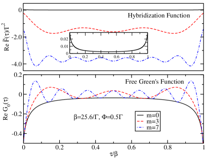
Figure 1: (color online) Imaginary-time data used as input for the CT-QMC solvers for different values of the imaginary voltage $\varphi_{m}$. The upper panel shows the non-trivial contribution $\tilde{F}(\tau)$, Eq. (21) to the hybridization function $F(\tau)$, the lower panel shows the imaginary-time Green’s function $G_{0}$. Raising $\varphi_{m}$ leads to increasingly oscillating imaginary-time Green’s functions and hybridization functions. The oscillations need to be resolved well by the QMC solver in order to guarantee an unbiased solution. As implied by Eq. (19) a strong negative shift $-c_{1}/2$ occurs in the hybridization function when sweeping through the region $\varphi_{m}\gg\Phi$. The imaginary parts $\mathrm{Im}\,F(\tau)$ and $\mathrm{Im}\,G_{0}(\tau)$ are small and also show oscillations.

III.2 Imaginary-Time Data

Typical input data for both, the weak-coupling and the strong-coupling approach, are shown in Fig. 1. With increasing imaginary voltage $\varphi_{m}$, oscillations with $m$ nodes occur in both, the imaginary-time Green’s function and the hybridization function. Moreover, the shift (19) grows quadratically, introducing a strong shift of the hybridization function towards negative values.

The strongly oscillatory behavior for large $\varphi_{m}$ makes a correspondingly fine resolution of the imaginary-time interval necessary. In a standard Hirsch-Fye algorithm Hirsch86 , the interval $[0,\beta)$ has to be represented by a comparatively small and fixed number of equidistant mesh points, i.e.  these oscillations cannot be adequately resolved. This limitation does not apply to CT-QMC, and it is hence the method of choice to access also large $\varphi_{m}$.

III.3 Phase Problem

In contrast to the equilibrium case, complex sampling weights $w_{c}=e^{i\gamma}|w_{c}|$ are obtained in both the weak-coupling and strong coupling formulation. As usual, one uses the modulus $|w_{c}|$ of the weight to determine the acceptance probability, while the phase $e^{i\gamma}$ has to be treated as additional observable. Usually, such an approach leads to a sign problem and severely limits the applicability of the Monte-Carlo simulations. Therefore, we must anticipate a generalized sign problem, i.e. $\langle e^{i\gamma}\rangle\to 0$ exponentially or worse. The situation is especially problematic for the hybridization expansion due to the additional shift (19) towards negative values. Indeed, as illustrated in Fig. 2 the sign problem becomes increasingly severe with increasing imaginary voltage $\varphi_{m}$, limiting this algorithm to small $\varphi_{m}$. From Fig. 2 it also becomes clear that the sign problem in the weak-coupling CT-QMC simulations is much milder and this approach allows us to simulate impurity models with large $\varphi_{m}$.

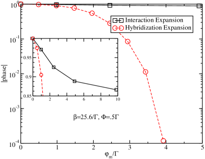
Figure 2: (color online) Absolute values of the average sampling weight phases $|\langle w_{c}/|w_{c}|\rangle|$ and $|\langle w_{\tilde{c}}/|w_{\tilde{c}}|\rangle|$ (Eqs. (14) and (15)) of the weak-coupling (solid lines) and the strong-coupling (dashed lines) solver, respectively, as a function of the imaginary voltage. On a logarithmic scale, the average phase decays faster than linearly for the strong-coupling approach when $\varphi_{m}$ is increased. No strong dependence on $\varphi_{m}$ is found for the weak-coupling algorithm.

To demonstrate the quality of the imaginary-time data which can be obtained with the weak-coupling CT-QMC method, we show in Fig. (3) the imaginary part of the Matsubara axis self-energy computed for $U=10\Gamma$, $\Phi=0.018\Gamma$, $T/\Gamma=0.0098$ and $\varphi_{m}=0$ ($m=0$), $\varphi_{m}/\Gamma=1.23$ ($m=10$), $\varphi_{m}/\Gamma=2.46$ ($m=20$), and $\varphi_{m}/\Gamma=3.69$ ($m=30$). The equilibrium Kondo temperature for this parameter set is $T_{\rm K}/\Gamma\approx 0.018\ll 1$, i.e. we are reasonably deep in the Kondo regime of the Anderson model. Moreover, the values for $\Phi$ and $T$ are such that $T\approx T_{\rm K}/2$ and $\Phi\approx T_{\rm K}$, i.e. precisely in the parameter region which is hard or impossible to access for other methods. Even for large complex voltage the accuracy of the numerical data is very good (error bars on the order of the line width) for both small and large Matsubara frequencies. In contrast to the results presented in Ref. Han07, , which are based on discrete-time Hirsch-Fye simulations, no discontinuities are observed for $\omega_{n}\approx\pm\varphi_{m}/2$ in the CT-QMC data. We note, however, that a recent preprint hanpreprint reports a trick by use of which this issue could be resolved within the discrete-time formalism.

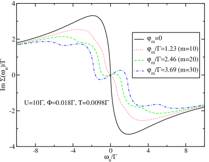
Figure 3: (color online) Imaginary part of the impurity self-energy obtained with the weak-coupling CT-QMC solver for $V_{G}=0$, $U/\Gamma=10$, $T/\Gamma=0.0098$ and $\Phi/\Gamma=0.018$ . The equilibrium Kondo scale here is $T_{\rm K}/\Gamma\approx 0.018$. We easily obtain high-quality data for all values $m=10$, $20$ and $30$ of the complexified voltage, even in this most challenging parameter regime $T_{\rm K}\ll\Gamma$, $\Phi\approx T_{\rm K}$ and $T\approx T_{\rm K}/2$. Each $m$-value was run on a single Intel Xeon(R) E5345 CPU for approx. 24 hours, so the data were obtained with relatively moderate computational effort.

IV Analytic Continuation

IV.1 Analytic Structure

As noted in Ref. Han07 , at finite interaction, branch cuts occur for $\mathrm{Im}\,z_{\omega}=\frac{\gamma}{2}\mathrm{Im}\,z_{\varphi}$ ($\gamma$ odd) in the complexified Green’s function $G(\mathrm{i}\varphi_{m}\to z_{\varphi},\mathrm{i}\omega_{n}\to z_{\omega})$. Introducing the complex vector variable $\underline{z}=(z_{\varphi},z_{\omega})$ we hence assume the Green’s function to be holomorphic as a function of two complex variables in domains $T^{C^{s}_{\nu}}:=\mathbb{R}^{2}+\mathrm{i}C^{s}_{\nu}$, where for $\nu\in 2\mathbb{Z}$

$$C^{s}_{\nu}:=\left\{\begin{pmatrix}a\\ b\end{pmatrix}\in\mathbb{R}^{2}:sa>0\,\wedge\,\frac{\nu-1}{2}|a|<b<\frac{\nu+1}{2}|a|\right\}$$

are the cones emerging from the branch cut condition for positive ($s=+1$) or negative ($s=-1$) imaginary voltages (see illustration in Fig. 4). Note that domains like $T^{C^{s}_{\nu}}$ are well-known objects in the theory of functions of several complex variables and are called tubular cone domains. For a good introduction see, e. g., Ref. encyclMathSciences .

In Ref. Han07 this structure is described by the Cauchy representation

$$\Sigma(\mathrm{i}\varphi_{m},\mathrm{i}\omega_{n})\approx\sum_{\gamma\in 2\mathbb{Z}+1}\int\,\mathrm{d}\varepsilon\,\frac{\sigma_{\gamma}(\varepsilon)}{\mathrm{i}\omega_{n}-\frac{\gamma}{2}(\mathrm{i}\varphi_{m}-\Phi)-\varepsilon}$$ (22)

for the corresponding self-energy. However, Eq. (22) is only approximate, because the $\mathrm{i}\varphi_{m}$-dependence of the functions $\sigma_{\gamma}(\varepsilon)$ is not taken into account. Such a non-trivial dependence appears as a result of higher-order corrections in $U$.

Let us start by discussing the analytically continued bare Green’s function

$$G_{0}(z_{\varphi},z_{\omega})=\sum_{\alpha=\pm 1}\frac{\Gamma_{\alpha}/\Gamma}{z_{\omega}-\frac{\alpha}{2}(z_{\varphi}-\Phi)+\mathrm{i}\Gamma^{(\alpha)}(z_{\phi},z_{\omega})},$$ (23)

with $\Gamma^{(\alpha)}(z_{\varphi},z_{\omega}):=\Gamma\mathrm{sgn}(\mathrm{Im}\,z_{\omega}-\alpha\mathrm{Im}\,z_{\varphi}/2)$.

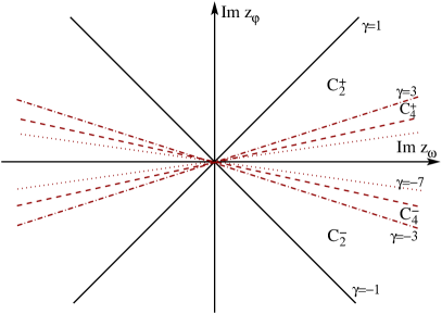
Figure 4: (color online) Geometric structure of the complex space carrying the two-variable Green’s function $G(z_{\varphi},z_{\omega})$. Branch cuts occur for $\mathrm{Im}\,z_{\varphi}=\frac{2}{\gamma}\mathrm{Im}\,z_{\omega}$, with $\gamma=\pm 1$ (solid lines), for $U=0$, but also at $\gamma=\pm 3$ (dash-dotted lines), $\gamma=\pm 5$ (dashed lines), $\gamma=\pm 7$ (dotted lines), and so on, for $U\neq 0$. Concentrating on the retarded sector of the Green’s function, $\mathrm{Im}\,z_{\omega}>0$, we introduce the cones $C^{\pm}_{\nu}$ bounded by the branch cuts with imaginary-part ratios $\frac{2}{\nu-1}$ and $\frac{2}{\nu+1}$. Adding the real subspaces $(\mathrm{Re}\,z_{\varphi},\mathrm{Re}\,z_{\omega})$, the tubular cones $T^{C^{\pm}_{\nu}}=\mathbb{R}^{2}+\mathrm{i}C^{\pm}_{\nu}$ are obtained as domains of holomorphy.

The corresponding geometric structure of the complex space is depicted in Fig. 4, the branch cuts given by the black lines $\gamma=\pm 1$. Note that the Green’s function does not vanish for all directions within a given $T^{C^{s}_{\nu}}$ as $\left|\underline{z}\right|\to\infty$. On the other hand, $\mathrm{Im}\,G_{0}(\underline{z})$ is at least bounded, and we assume that nonzero interactions do not alter this fundamental property. One can thus always find a constant $c$ such that the imaginary part of the function $f(\underline{z}):=G(\underline{z})+\mathrm{i}c$ is positive. Integral representations of the form $\int f(\zeta)K(z,\zeta)\,\mathrm{d}\zeta\,=f(z)$ which are valid for the class of holomorphic functions with non-negative imaginary part also hold for $G(\underline{z})$, since $-\mathrm{i}c\cdot\mathrm{const}(z)$ is also a function with non-negative imaginary part. This class of functions on tubular cone domains was extensively studied by mathematicians. In Ref. Vladimirov1978 , Vladimirov finds a generalization of Herglotz-Nevanlinna representations Nevanlinna to such domains. See Appendix A for details.

The validity of the imaginary-voltage formalism is presently based on the assumption of asymptotic convergence of the perturbation series in $U$. Thus, the influence of the branch cut between $T^{C^{s}_{\nu+2}}$ and $T^{C^{s}_{\nu}}$ is expected to become negligible as $\nu\to\infty$, i.e. all branch cuts with $\nu>\nu_{\text{crit}}$ can be ignored. The maximal value $\nu_{\text{crit}}$ may for example be estimated from the expansion order histogram of the weak-coupling QMC simulation, since a given branch cut with index $\gamma=\nu+1$ is only established by diagrammatic contributions with order larger than a certain value $n$, which is roughly proportional to $|\gamma|$.

As stated in Ref. Han07 we are required to first take the limit $z_{\varphi}\to\Phi$ and then $z_{\omega}\to\omega+\mathrm{i}0^{+}$. In our language, the spectral function is given by

$$A(\omega)=-\frac{1}{\pi}\lim_{\nu\to\infty}\lim_{\underline{z}\to(\Phi,\omega)}\mathrm{Im}\,G_{(\nu)}(\underline{z}).$$ (24)

Since branch cuts with index $\gamma\geq\nu_{\text{crit}}+1$ vanish we choose the domain $T^{C_{\varepsilon}}$ with

$$C_{\varepsilon}:=\{(x_{1},x_{2})\in\mathbb{R}^{2}\,|\,x_{2}>0\wedge-\varepsilon x_{2}<x_{1}<\varepsilon x_{2}\},$$ (25)

and $\varepsilon\approx\frac{2}{\nu_{\text{crit}}-1}$ for the analytic continuation of the interacting Green’s function. This choice of domain is illustrated in Fig. 5. In practice, the critical branch cut is yet chosen arbitrarily but to be small, see section IV.2.

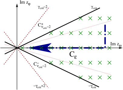
Figure 5: (color online) Sketch of the geometry of the two-dimensional analytic continuation problem. For the critical domain index $\nu_{\text{crit}}$ the branch cut $\gamma_{\text{crit}}+2=\nu_{\text{crit}}+1$ (dotted line) is negligible, while the critical branch cuts $\pm\gamma_{\text{crit}}$ are not. The Green’s function is therefore holomorphic in the cone domain $T^{C_{\varepsilon}}$ bounded by the ratios $\pm\mathrm{Im}\,z_{\varphi}=\frac{2}{\gamma_{\text{crit}}}\mathrm{Im}\,z_{\omega}=:\varepsilon\mathrm{Im}\,z_{\omega}$, with $C_{\varepsilon}$ given by Eq. (25). Investigating the Green’s function at the edge of this domain is compatible with the limiting procedure of taking $z_{\varphi}\to\Phi$ and then $z_{\omega}\to\omega+\mathrm{i}0^{+}$ for the spectral function $A(\omega)$. This is indicated by the bold dash-dotted arrow. Using the integral representation (26), a most likely limit of the Green’s function at the edge, $\lim_{\underline{\zeta}\to\underline{x}}{G}(\underline{z})$, $\underline{x}\in\mathbb{R}^{2}$, will be inferred from the QMC data $\left.G(\mathrm{i}\varphi_{m},\mathrm{i}\omega_{n})\right|_{T^{C_{\varepsilon}}}$ in the domain using a Maximum Entropy Method (Sec. IV.2). The spatial locations of the QMC data points in the domain are symbolized by the crosses. In the case of strong interaction, for small Matsubara frequencies we are limited to small values of $\varphi_{m}$.

As shown in Appendix A the Poisson kernel representation resulting from Vladimirov’s theorem is

$$\left.\mathrm{Im}\,G(\underline{z})\right|_{T^{C_{\varepsilon}}}=\int_{\mathbb{R}^{2}}\mathrm{d}^{2}x\,\mathcal{P}_{\varepsilon}(\underline{z}-\underline{x})\lim_{\underline{\zeta}\to\underline{x}}\left.\mathrm{Im}\,G(\underline{\zeta})\right|_{T^{C_{\varepsilon}}}$$ (26)

with

$$\mathcal{P}_{\varepsilon}(\underline{z})=\frac{1}{\pi^{2}\varepsilon}\prod_{\mu=\pm 1}\frac{y_{2}-\mu y_{1}/\varepsilon}{(x_{2}-\mu x_{1}/\varepsilon)^{2}+(y_{2}-\mu y_{1}/\varepsilon)^{2}},$$ (27)

where $\underline{x}$ and $\underline{y}$ are the real and imaginary parts of $\underline{z}$.

IV.2 Maximum Entropy Method

IV.2.1 Single Analytic Continuation

The numerical analytic continuation of imaginary-time quantum Monte Carlo data is a highly ill-posed problem. Even if the finite set of QMC data did not contain any stochastic noise there would exist an infinite-dimensional manifold of solutions to the integral equation associated with the continuation, i.e. the spectral representation

$$G(\mathrm{i}\omega_{n})=\int\,\mathrm{d}\varepsilon\,\frac{A(\varepsilon)}{\mathrm{i}\omega_{n}-\varepsilon}=:K_{\text{eq}}[A](\omega_{n})$$ (28)

for the conventional continuation problem.

Hence, a regularization procedure picking a “most probable” solution is required. Typically, this is approached with a Maximum Entropy Method (MEM), a rigorous framework rooted in Bayesian logic which can be understood as an automatic Ockham’s Razor, in the sense of being “maximally noncommittal with regard to missing information” jarrell_review ; maxent_buch ; jaynes57 . The spectral function $A(\omega)$ is interpreted as a probability distribution. A default model $D(\omega)$ is introduced as a-priori information about the solution $A(\omega)$. Additional information, given by the measured imaginary-time data $\bar{G}(\mathrm{i}\omega_{n})$, is inferred through the kernel $K_{\text{eq}}[A]$ in (28). If there is no additional information the procedure will pick $A(\omega)=D(\omega)$, in Bryan’s MEM algorithm bryan .

In practice, a functional

$$Q[A]=\chi^{2}[A]-\alpha S[A],\quad\alpha>0$$ (29)

is minimized in the space of candidate solutions for a given hyper-parameter $\alpha$. The QMC data must be Gaussian distributed, such that the likelihood penalty $\chi^{2}[A]$ is given by

$$\chi^{2}[A]=\frac{1}{2}\sum_{\rho,\eta=1}^{N}(\bar{G}_{\rho}-K_{\text{eq}}[A]_{\rho})C^{-1}_{\rho\eta}(\bar{G}_{\eta}-K_{\text{eq}}[A]_{\eta}),$$ (30)

where $\bar{G}_{\eta}$ are the measured mean real or imaginary parts of the imaginary-frequency Green’s function $G(\mathrm{i}\omega_{n})$, and $C^{-1}_{\rho\eta}$ are the elements of the inverse covariance matrix.

The default model $D(\omega)$ is invoked through the entropy

$$S[A]=\int\,\mathrm{d}\varepsilon\,\left[A(\varepsilon)-D(\varepsilon)-A(\varepsilon)\log\frac{A(\varepsilon)}{D(\varepsilon)}\right].$$ (31)

For a detailed theoretical justification of this choice for the entropy see Ref. maxent_buch .

The easiest way of fixing the regularization parameter $\alpha$ is to employ the condition $\chi^{2}\approx N$ (historic MEM). It is, however, more reasonable to calculate a posterior probability distribution $\mathrm{Pr}(A|\alpha)$. Setting $\alpha$ to the maximum of the posterior probability distribution is called classic MEM. Marginalizing $\alpha$ by choosing $\mathrm{Pr}(A|\alpha)$ as weights for $A$ when integrating over $\alpha$ is empirically found to be most suitable and is also most justified from the theoretical point of view (Bryan’s MEM).

IV.2.2 Double Analytic Continuation

In order to adapt the above procedure to the double analytic continuation problem, a non-negative quantity has to be found which

1. uniquely represents any possible function in the data range of interest – say $T^{C_{\varepsilon}}$ – in order to define a $\chi^{2}$ for inference;

2. easily allows calculating the non-equilibrium spectral function $A(\omega)$.

We choose

$$\tilde{A}(\underline{x}):=-\frac{1}{\pi}\lim_{\underline{\zeta}\to\underline{x}}\left.\mathrm{Im}\,G(\underline{\zeta})\right|_{T^{C_{\varepsilon}}}$$ (32)

as such a representation, since due to the Kramers-Kronig relations and the validity of the representation (26), $\tilde{A}$ yields a unique and simple representation of all possible functions $G|_{T^{C_{\varepsilon}}}$. The non-equilibrium spectral function is easily accessible, since $A(\omega)=\tilde{A}(\Phi,\omega)$.

In the case of zero interaction,

$$\tilde{A}_{0}(\underline{x})=-\frac{1}{\pi}\mathrm{Im}\,\sum_{\alpha=\pm 1}\frac{\Gamma_{\alpha}/\Gamma}{x_{2}-\alpha(x_{1}-\Phi)/2-\varepsilon_{d}+\mathrm{i}\Gamma}.$$ (33)

It is easy to verify that $\tilde{A}_{0}(\underline{x})$ is a positive function with $\int\mathrm{d}^{2}x\tilde{A}(\underline{x})=l$ if one constrains the $x_{1}$-integration to an arbitrary finite interval of length $l$. This fact and the fact that $\tilde{A}(\Phi,\omega)=A(\omega)\geq 0$ do not imply $\tilde{A}(x_{1},x_{2})\geq 0$ in general. We however assume $\tilde{A}(x_{1},x_{2})\geq 0$ and expect to obtain revealing signatures within the MEM, in case the real $\tilde{A}$ is not positive definite for a given data set. Note that even in the presence of regions where $\tilde{A}<0$, a MEM can be implemented, by identifying the nodes of $\tilde{A}$, as in the case of bosonic spectral functions. In general, positivity may be enforced by adding a positive real constant $b$ to the spectral function and adding a corresponding term to the image. As particular example for this procedure, we quote here the case of the Nambu off-diagonal Green’s function $G_{12}$, where the positivity is enforced as $G_{12}(\tau)+b\int\,\mathrm{d}\omega\,K(\tau,\omega)=\int\,\mathrm{d}\omega\,K(\tau,\omega)(A_{12}(\omega)+b)$ jarrell .

We hence choose (26) as a kernel function for the $\chi^{2}$ functional and only take data in $T^{C_{\varepsilon}}$ into account. The entropy expression (31) is adopted for a two-dimensional default model $\tilde{D}(\underline{x})$.

IV.2.3 Implementation

First note that since the input data for the Poisson kernel (26) are obtained from statistically independent QMC simulations, the covariance $C$ in the $\chi^{2}$ functional (30) has a block-diagonal shape

$$C=\begin{pmatrix}C^{(m_{\text{min}})}&0&\cdots&\\ 0&C^{(m_{\text{min}}+1)}&0&\cdots\\ \vdots&0&\ddots&\\ &\cdots&0&C^{(m_{\text{max}})}\\ \end{pmatrix}.$$ (34)

The submatrices $C^{(m)}$ are covariances for the subset of data $G(\mathrm{i}\varphi_{m},\mathrm{i}\omega_{n})$ at a fixed $\varphi_{m}$, estimated from the output of the corresponding equilibrium QMC simulation.

Our implementation of the Maximum Entropy Method is based on Bryan’s standard algorithm introduced in Ref. bryan . A singular value decomposition (SVD) of the kernel

$$K:V_{\tilde{A}}\to V_{\text{data}},\quad K=V\Sigma U^{T}$$ (35)

is performed, with $V$, $U^{T}$ orthogonal, and the singular values

$$\Sigma=\mathrm{diag}(\sigma_{1},\sigma_{2},\dots,\sigma_{s},0,\dots,0),$$ (36)

$\sigma_{1}\geq\sigma_{2}\geq\dots\geq\sigma_{s}>0$. Many important quantities may be reduced to the $s$-dimensional singular space $V_{\Sigma}$. Most notably, the $(\dim V_{\tilde{A}})$-dimensional optimization problem given by

$$Q[\tilde{A}]\stackrel{{\scriptstyle!}}{{=}}\text{min}$$ (37)

may be solved within the singular space using Levenberg-Marquardt iterations. As $s$ is comparably small after truncating the singular space with respect to the floating point precision of the singular values $\sigma_{i}$ (typically, $s\approx 50$), the algorithm is still sufficiently efficient, even though a two-dimensional frequency grid is required for the numerical resolution of $\tilde{A}$, and hence $\mathrm{dim}\,V_{\tilde{A}}\geq 10^{5}$.

The algorithm enables us to calculate several important data qualifiers and posterior probabilities and therefore to classify both input data quality and candidate solutions. The posterior

$$\mathrm{Pr}(\alpha|\bar{G})=\mathrm{Pr}(\alpha)\int\mathcal{D}\tilde{A}\,\frac{\mathrm{e}^{Q}}{Z_{L}Z_{S}(\alpha)},$$ (38)

with $Z_{L}=\int\mathcal{D}[K\tilde{A}]\,\mathrm{e}^{-\chi^{2}/2}$, $Z_{S}(\alpha)=\int\mathcal{D}\tilde{A}\,\mathrm{e}^{\alpha S}$, and the Jeffreys prior Jeffreys46 $\mathrm{Pr}(\alpha)\propto\alpha^{-1}$, is calculated using a Gaussian approximation for $Q$, centered around the solution $\tilde{A}_{\text{opt},\alpha}$ of Eq. (37).

The usual procedures and strategies for data qualification and improvement of results as described in jarrell_review are adopted: Assuming a flat prior $\mathrm{Pr}(\tilde{D})$, the posterior for the default model

$$\mathrm{Pr}(\tilde{D}|\bar{G})\propto\int\,\mathrm{d}\alpha\,\int\mathcal{D}\tilde{A}\,\mathrm{Pr}(\alpha)\frac{\mathrm{e}^{Q}}{Z_{L}Z_{S}(\alpha)}$$ (39)

is computed easily. $\mathrm{Pr}(\tilde{D}|\bar{G})$ serves as evidence for the quality of prior information when comparing within sets of default models for given QMC data. Whereas a posterior probability for the domain parameter $\varepsilon$ for given data and given default model, $\mathrm{Pr}(\varepsilon|\bar{G},\tilde{D})$, would be a sensible extension to the algorithm, we have not derived it yet. Useful ingredients might be found in the literature on blind deconvolution in signal processing, see pinchas05 . In our implementation, a small enough $\varepsilon$ is chosen a priori.

Picking appropriate data sets with well-estimated covariance from the QMC output is also a non-trivial part of the problem. A good check is to determine the most probable mock error rescaling $\sigma$ where the covariance $C$ is formally substituted by $\sigma^{2}C$. If the most probable $\sigma$ (“merit”), i.e. the solution of

$$\frac{\chi^{2}_{\text{classic}}}{\sigma^{2}}+N_{g}=N$$ (40)

deviates from 1 by more than a few tens of percent, the input data are rejected jarrell_review . $\chi^{2}_{\text{classic}}$ is the $\chi^{2}$ value of the classic MEM solution, the number of data points $N$, and the number of “good” data points $N_{g}=\sum_{i}\frac{\lambda_{i}}{\alpha_{\text{classic}}+\lambda_{i}}$ with $\lambda_{i}$ the eigenvalues of

$$\Lambda_{ij}=\left[\sqrt{\tilde{A}_{i}}\frac{\partial^{2}\chi^{2}/2}{\partial\tilde{A}_{i}\partial\tilde{A}_{j}}\sqrt{\tilde{A}_{j}}\right]_{\tilde{A}_{\text{classic}}}.$$ (41)

In practice, a maximal Matsubara frequency $n_{\text{max}}$ compatible with the error rescaling merit was determined, and all data $\mathrm{Im}\,G(\mathrm{i}\varphi_{m},\mathrm{i}\omega_{n})$ in $T^{C_{\varepsilon}}$, with $n\leq n_{\text{max}}$ were used for inference. Presumably, better data selection strategies do exist. For example, using independent measurements for $\mathrm{Re}\,G$ and taking them into account by using a Schwarz representation (see Appendix A) could yield better results. Furthermore, the largest Matsubara frequency index $n_{\text{max}}$ could be determined for each $\varphi_{m}$ individually. The latter appears to be necessary for non-equilibrium data.

For the truncation of singular values, a threshold $\lambda$ was used,

$$\sigma_{i}\mapsto\begin{cases}\sigma_{i},&\text{if }\sigma_{i}\geq\lambda\sigma_{1}\max\{M,N\},\\ 0,&\text{else}\end{cases}$$ (42)

for an $M$ by $N$ kernel matrix. While for the conventional Wick rotation $\lambda\approx 10^{-8}$ was sufficient, $\lambda\approx 10^{-12}$ had to be chosen in our case in order to take all relevant search directions in the $\tilde{A}$ space into account. Quadruple precision floating point arithmetic was found to be unnecessary. For discretizing the $\tilde{A}(\underline{x})$ function, logarithmic meshes for the $x_{1}$ and $x_{2}$ variables were used. Although $\tilde{A}(\underline{x})$ does not decay for all directions as $\underline{x}\to\infty$, choosing a finite mesh and truncating the integrals was not found to be critical.

IV.2.4 Equilibrium

As a test case we consider the equilibrium limit $\Phi=0$. The data for $\varphi_{m}=0$ can be analytically continued with the standard Wick rotation, using Eq. (28) and the standard MEM. Figure 6 compares this 1D spectral function to the result based on the 2D data set $G(\mathrm{i}\varphi_{m},\mathrm{i}\omega_{n})$ and continued using the domain $T^{C_{\varepsilon}}$ and the kernel function defined in Eq. (26). As default models for high temperatures we use Lorentzians with variable width $\Gamma_{\text{default}}$. They read

$$D(\omega)=\frac{1}{\pi}\frac{\Gamma_{\text{default}}}{\omega^{2}+\Gamma_{\text{default}}^{2}}$$ (43)

for the 1D continuation and

$$\tilde{D}(x,\omega)=\frac{1}{\pi}\frac{\tilde{\Gamma}_{\text{default}}(x)}{\omega^{2}+\tilde{\Gamma}_{\text{default}}(x)^{2}}$$ (44)

for the 2D continuation, with $\tilde{\Gamma}_{\text{default}}(x)=\sqrt{\Gamma_{\text{default}}^{2}+x^{2}}$. An annealing procedure in the temperature was used for both, the 1D and 2D data for invoking adequate prior information, i.e. we used the $\tilde{A}$ solution of the next higher temperature as default model, starting with the Lorentzian at the highest temperature.

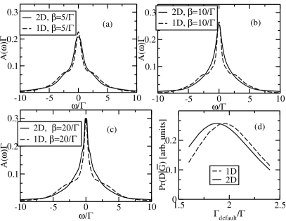
Figure 6: Analytically continued data for equilibrium ($\Phi=0$) obtained using the conventional Wick rotation (1D) and the unconventional two-variable continuation (2D), with $U=5\Gamma,V_{G}=0$. The domain parameter for 2D continuation is $\varepsilon=\frac{2}{19}$. Subfigure (d) shows the posterior probabilities $\mathrm{Pr}(D|\bar{G})$ of the default models as a function of $\Gamma_{\text{default}}$ (Eqs. (43) and (44)).

This default model selection procedure appears not to have any strict Bayesian justification, however the physical argument is freezing out the high-frequency degrees of freedom and using present data for inferring low-energy details of the spectrum step by step jarrell . A similar idea plays the key role in several modern renormalization group techniques. Note that Gaussian default models are not well-suited for our data, since the high-frequency tail in the wide-band limit is Lorentzian. This manifests itself quantitively in the following way: For the Gaussian default models we tested all had $\mathrm{Pr}(\tilde{D}|\bar{G})$ one order of magnitude lower than the Lorentzian ones. For both, the Gaussian and the Lorentzian, we can expect the quantity $\Gamma_{\text{default}}/\Gamma$ to be $>1$, due to the overall broadening introduced by a finite interaction $U$.

Indeed, for the parameters $U=5\Gamma,V_{G}=0$, $\Phi=0$ shown in Fig. 6(d), the (unnormalized) posterior probabilities $\mathrm{Pr}(D|\bar{G})$ and $\mathrm{Pr}(\tilde{D}|\bar{G})$ as a function of the parameter $\Gamma_{\text{default}}$ are peaked at $\approx 2\Gamma$ for both, the 1D and 2D continuation procedures, respectively. These probabilities were calculated for $\beta\Gamma=10\Gamma$. The most probable $\Gamma_{\text{default}}$ was chosen as default model. However, a strong dependence of the results on $\Gamma_{\text{eff}}$ was not observed.

The spectral functions shown in Fig. 6 were obtained for $\beta\Gamma=5$, $10$, and $20$. We chose $\varepsilon=\frac{2}{19}$ for the 2D domain, using $n_{\text{max}}=10$, $20$, $40$ for $\beta\Gamma=5$, $10$, and $20$, respectively. Note that due to the simple data selection strategy described in the previous section we only took into account data points with $\varphi_{-2}\leq\varphi_{m}\leq\varphi_{2}$. Using a global $n_{\text{max}}$, the estimate for the covariance submatrix $C^{(m=0)}$ in Eq. (34) eventually becomes singular, even though $C^{(m)}$ with $|m|\geq 3$ and $\omega_{n}>\omega_{n_{\text{max}}}$ could still be estimated for a limited set of Matsubara frequencies. We expect that using such additional, well-estimated $C^{(m)}$ might lead to more structured spectral functions. In practice, however, the merit $\sigma$ must yet be viewed as a rather crude measure of the quality of the covariance estimate. So for the purpose of both simplicity and reproducibility we used the stronger restriction.

The Kondo temperature for $U=5\Gamma$ is $T_{\rm K}/\Gamma\approx 0.1$, i.e. we can expect first signatures of strong coupling physics like Hubbard bands and a temperature dependent quasi-particle peak of reduced width in the spectra. Indeed both the 1D and 2D MEM reproduces these features. More importantly, the overall shape of the spectra obtained agrees for all temperatures shown in Fig. 6(a-c). The results depend only slightly on the choice of $\Gamma_{\text{default}}$ for relevant values of $\mathrm{Pr}(\tilde{D}|\bar{G})$. Although the spectra inferred from the 2D procedure using our current implementation appear to be less structured, the overall shape seems to be reconstructed quite well. For more serious calculations, the detailed high-frequency behavior (and behavior for large $x$) should be introduced with a more sophisticated default model, e.g. based on perturbation theory.

IV.2.5 Inferred Representation

Figure 7 shows the Lorentzian default model we used at the highest temperature in the annealing procedure, $\beta\Gamma=2$. At the lowest temperature $\beta\Gamma=20$, the representation shown in Fig. 8 was obtained. The equilibrium spectral function shown in Fig. 6(c) is given by the cut $\tilde{A}(\Phi=0,\omega)$. Other values of $\mathrm{Re}\,z_{\varphi}$ do not have any physical meaning.

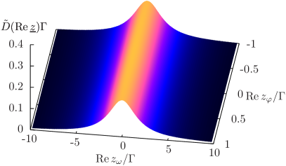
Figure 7: (color online) Lorentzian default model (44) with best $\mathrm{Pr}(\tilde{D}|\bar{G})$ for first annealing step in equilibrium.

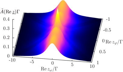
Figure 8: (color online) MEM solution for $\tilde{A}$ inferred from the QMC data at the lowest temperature, $\beta\Gamma=20$, for the equilibrium test case shown in Fig. 6.

Note that certain structures appear in the inferred $\tilde{A}(x,y)$ which vary as the domain parameter $\varepsilon$ is changed: they occur for $\mathrm{Re}\,z_{\varphi}=\pm\mathrm{Re}\,\varepsilon z_{\omega}$. We interpret them as resulting from the properties of the kernel function discussed in Sec. IV.2.8 in combination with the MEM principle of only incorporating changes which are strongly supported by data. Also, at larger distance from the origin, discretization errors from the discretization of the double integral are most dominant for this most structured region of the kernel. At finite bias, the qualitative structure of the inferred representation remains unchanged.

IV.2.6 Finite Bias

The rule of thumb $n_{\text{max}}\approx\frac{\beta U}{2}$ appeared to be a good choice for preparing the equilibrium QMC data for inference. For $\Phi>0$ a first interesting observation is that at sufficiently low temperatures $n_{\text{max}}$ seems to be considerably smaller than $\frac{\beta U}{2}$.

In fact, the simple data selection strategy yielding $n_{\text{max}}$ does not appear to produce a sufficiently informative data set to obtain quantitative agreement with for example RT-MC calculations Werner10 . We observed this problem for $\beta\Gamma=10$ and the interaction strengths $U=4\Gamma$ and $U=6\Gamma$ and several values of the bias voltage $\Phi$. On the other hand, by picking an $n_{\text{max}}$ for each $\varphi_{m}$ separately, we found larger sets of admissible input data, which tend to show a good agreement with RT-MC data for the current-voltage characteristics. While the procedure is yet somewhat arbitrary, the following criteria were used to restrict the choices of data sets producing convergent MEM solutions:

• ensure an error rescaling $\sigma\approx 1$;

• discard strongly oscillating solutions and solutions with obvious artifacts around $\omega\approx 0$;

• discard solutions which strongly violate the physical sum rule $\|A\|:=\int\,\mathrm{d}\omega\,A(\omega)=1$. In many cases, too small values $\|A\|\approx 0.9$ were obtained. Note that the MEM as we implemented it only has prior information about the value of the truncated double integral $\iint\mathrm{d}^{2}x\tilde{A}(\underline{x})$, because two-dimensional probability densities are considered when the entropy expression (31) is straightforwardly generalized with respect to $\tilde{A}$;

• use as many data points as possible, starting with small $\omega_{n}$, to maximize the amount of accessible information.

Note that the domain parameter $\varepsilon$ was, again, chosen somewhat arbitrarily: For $U=4\Gamma$ we only investigated $\nu_{\text{max}}=16$, for $U=6\Gamma$ we picked $\nu_{\text{max}}=20$, with $\varepsilon=\frac{2}{\nu_{\text{max}}-1}$. The dependence of the results on the particular choice of $\varepsilon$ was not studied systematically yet, but work along these lines is under way and the results will be presented elsewhere. The usual annealing procedure with temperatures $\beta\Gamma=2$, $\beta\Gamma=5$, $\beta\Gamma=10$, where for $\beta\Gamma=2$ the Lorentzian default models with $\Gamma_{\text{default}}=1.5\Gamma$ ($U=4\Gamma$) and $\Gamma_{\text{default}}=2.1\Gamma$ ($U=6\Gamma$) were found to be most suitable based on the posterior $\Pr(\tilde{D}|\bar{G})$.

The current $J$ was computed using Meir and Wingreen’s equation meirwingreen94

$$J=J_{\text{max}}\int\,\mathrm{d}\omega\,\left[f_{L}(\omega)-f_{R}(\omega)\right]A(\omega),$$ (45)

with $J_{\text{max}}=\frac{\Gamma e}{h}$.

Our experience up to now indicates that for too small sets of QMC data the method systematically underestimates the current, because Bryan’s algorithm by convention does not incorporate any changes to $\tilde{A}\approx\tilde{D}$ in case the data do not provide sufficient evidence for such modifications. As a result, the current is too small, because in the vicinity of $\omega\approx 0$ the less structured default model obtained from the next higher temperature (initially the broad Lorentzian (44)) is much flatter than the true solution, which features a sharp Abrikosov-Suhl resonance in the relevant frequency range. Hence, the spectral function obtained from the MEM has less spectral weight in the integration window in Eq. (45) than the true $A(\omega)$.

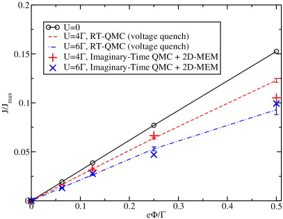
Figure 9: (color online) Current-voltage characteristics obtained using the 2D MEM compared to RT-QMC Werner10 data for indicated Coulomb interactions at temperature $\beta\Gamma=10$.

Due to this trend of underestimation, in Fig. 9 we compare the largest values of the current compatible with the above-listed restrictions to data obtained using a recently developed RT-MC approach Werner10 . A generally good agreement is obtained. However, the data selection procedure is still too arbitrary to consider these results unbiased. Error bars are not available. If we only considered a fixed set of data $\bar{G}$, the covariance $\text{Cov}(\tilde{A}(\underline{x}^{(1)}),\tilde{A}(\underline{x}^{(2)}))$ would be estimated easily bryan . However, due to large off-diagonal terms, attempting to estimate an error bar for $J$ is rather cumbersome. The $\Phi/\Gamma=0.0625$ run did not converge to a solution meeting our criteria for $U=4\Gamma$.

IV.2.7 Non-Equilibrium Spectral Functions

Spectra resulting from the procedure described above are shown in Fig. 10. These are the spectral functions used to compute the current in Fig. 9. While oscillations appear, presumably due to the neglected error of the covariance estimate vonderlinden , it is evident that the overall spectral weight at small $\omega$ is larger for $U=4\Gamma$ than for $U=6\Gamma$ when $\Phi<0.5\Gamma$. This is consistent with the expectation that the quasi-particle resonance for $U=6\Gamma$ is already suppressed, because $\beta^{-1}=0.1>T_{K}$, whereas $\beta^{-1}\approx T_{K}$ for $U=4\Gamma$. In Fig. 11, we show a comparison of the spectral functions for $U/\Gamma=4$ and $\beta\Gamma=10$ to the result obtained from fourth-order perturbation theory fujiiueda03 . Based on the results presented in Ref. Werner10, , we expect that fourth-order perturbation theory is quite accurate at this interaction strength and temperature. Besides the unphysical oscillations in the MEM result and a bias towards the high-temperature default model, especially for larger voltage biases, the agreement between the spectral functions, in particular the qualitative distribution of the spectral weight, seems satisfactory.

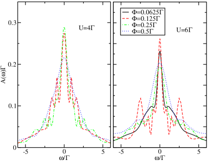
Figure 10: (color online) Spectra $A(\omega)=\tilde{A}(\Phi,\omega)$ used for the computation of the current shown in Fig. 9.

Table 1 shows the norm $\|A\|=\int A(\omega)\,\mathrm{d}\omega\,$ for the functions presented in the figure.

$\Phi/\Gamma$	$\|A\|_{U=4\Gamma}$	$\|A\|_{U=6\Gamma}$
0.0625	–	0.91
0.125	0.92	0.92
0.25	0.92	0.95
0.5	1.03	1.16

Table 1: Norms of the spectral functions shown in Fig. 10.

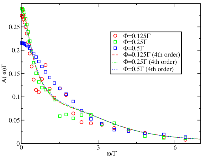
Figure 11: (color online) Spectra $A(\omega)=\tilde{A}(\Phi,\omega)$ for $U=4\Gamma$ as compared to fourth-order perturbation theory.

Obviously, the physical sum rule $\|A\|=1$ is not strictly obeyed, and there is a slight tendency towards too small norms whose origin is unclear but which appears to be consistent with the trend of current underestimation. Moreover, the selection of data we chose at $\beta\Gamma=10$ for $U=4\Gamma$ and $U=6\Gamma$ is shown in table 1 and table 3, respectively. The tables present the number $N_{m}\approx n_{\text{max}}(m)-2m/\varepsilon$ of Matsubara frequencies which are located within the cone domain $T^{C_{\varepsilon}}$ for the chosen $n_{\text{max}}(m)$.

$\Phi/\Gamma$	$N_{m=0}$	$N_{m=\pm 1}$	$N_{m=\pm 2}$	$N_{m=\pm 3}$
0.0625	–	–	–	–
0.125	26	12	6	3
0.25	24	12	5	3
0.5	24	12	6	3

Table 2: Number $N_{m}$ of Matsubara frequencies taken into account for each value of $m$ taken into account in the data selection at $\beta\Gamma=10$ for $U/\Gamma=4$ and for the voltages plotted in Fig. 9.

$\Phi/\Gamma$	$N_{m=0}$	$N_{m=\pm 1}$	$N_{m=\pm 2}$	$N_{m=\pm 3}$
0.0625	20	11	6	1
0.125	21	11	6	8
0.25	21	11	6	3
0.5	20	11	6	1

Table 3: Same as Table 1 but for $U/\Gamma=6$.

We did not consider larger values of $m$, although at least $m=\pm 4$ yields further relevant information about $\tilde{A}$. For a test case the spectra did not show dramatic qualitative changes as additional values at larger $\varphi_{m}$ were included, as long as the error scaling merit remained $\sigma\approx 1$. However, the level of arbitrariness in the data selection would have been even larger, because of the corresponding additional $n_{\text{max}}$ parameters.

Obtaining reliable spectral functions at finite bias will obviously require more effort and we will briefly comment on possible avenues for this effort in the Conclusion.

IV.2.8 Kernel Structure

We finish with some remarks about the structure of the kernel function (26) and its role in the continuation problem. In the language of Bayesian inference the kernel function defines the information channel through which evidence about the shape of the representation function $\tilde{A}(\underline{x})$ and thus also the physical spectral function $A(\omega)$ is extracted from the Monte Carlo data.

For the information provided by a single data point, this channel results in vague (strong) evidence for changes in a given compact region $R\subset V_{\tilde{A}}$, see Eq. (35), depending on whether the subset of column vectors $u_{i}$ of $U$ spanning $R$ is associated with small (large) singular values $\sigma_{i}$, and a small (large) overlap of the column vectors $v_{i}$ of $V$ with the data point. For this reason, very small singular values yield irrelevant components of the channel and are therefore projected out in Bryan’s algorithm by introducing the threshold $\lambda$, Eq. (42).

We can neither perform the SVD analytically, nor can we analytically take into account structural changes which occur when rotating the basis of $V_{\text{data}}$ to the eigenbasis of the covariance matrix $C$ in order to consider statistically independent data. We can however consider values of the kernel in $V_{\tilde{A}}$ for a given data point, assuming it to be uncorrelated with other data points so that it may be investigated separately. Within our QMC implementation, experience shows that correlations between Matsubara frequencies $\omega_{n}$, $\omega_{n^{\prime}}$ are monotonically decreasing as a function of distance $|\omega_{n^{\prime}}-\omega_{n}|$, though very slowly.

Let us first consider a single uncorrelated imaginary part of a Green’s function at Matsubara frequency $\omega_{n}$ in the standard Wick rotation problem. The spectral function $A(\varepsilon)$ is inferred through the Lorentzian-shaped kernel (28),

$$\mathrm{Im}\,K_{\text{eq}}[A(\varepsilon)](\omega_{n})=-\frac{\omega_{n}}{\varepsilon^{2}+\omega_{n}^{2}}.$$ (46)

For all $\omega_{n}$ the kernel (28) is centered around $\varepsilon=0$ and higher frequencies are associated to larger values of the kernel as the width given by $\omega_{n}$ is increased. As compared to $\varepsilon\approx 0$ the values of the kernel at large frequencies are still small. We can therefore expect large singular values and thus relevant components of the kernel to be associated with small frequencies only. This is in agreement with the well-known observation that high-frequency information about the spectral function is better put into the default model as prior knowledge and a good resolution is obtained for the – fortunately most interesting – low-frequency region.

In the case of our two-dimensional continuation the situation is quite similar. For given data $\mathrm{Im}\,G(\mathrm{i}\varphi_{m},\mathrm{i}\omega_{n})$ the Poisson kernel in Eq. (26) is

$$\frac{1}{\pi^{2}\varepsilon}\prod_{\mu=\pm 1}\frac{\omega_{n}-\mu\varphi_{m}/\varepsilon}{(x_{2}-\mu x_{1}/\varepsilon)^{2}+(\omega_{n}-\mu\varphi_{m}/\varepsilon)^{2}}.$$

It is the product of two Lorentzians. In analogy to the argument given above one may expect the best resolution for data $\tilde{A}(\underline{x}^{\text{(best)}})$ with

$$x_{2}^{\text{(best)}}\approx\pm x_{1}^{\text{(best)}}/\varepsilon\ \text{and }x_{2}^{\text{(best)}},x_{1}^{\text{(best)}}\approx 0.$$ (47)

This does not depend on the physical voltage $\Phi$, except that the critical branch cut index $\gamma_{\text{crit}}$ appears to be decreasing as a function of $\Phi$. This can be estimated from the expansion order histogram for the example shown in Fig. 12.

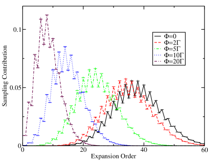
Figure 12: (color online) Expansion order histogram obtained using the weak-coupling solver for $K=-\beta U/4+1$, which suppresses the odd perturbation orders Werner10 . The results are for $U=7\Gamma$, $\beta\Gamma=51.2$, and $\varphi_{m}=2.46\Gamma$ for indicated voltages $\Phi$. The average order decreases as $\Phi$ is increased. A similar behavior is obtained for different values of $\varphi_{m}$ and $U$.

Consequently, the domain parameter $\varepsilon$ could presumably be raised as $\Phi$ be increased. However, in the limit of very large voltages, especially the low-frequency region of the physical spectrum $A(\omega)=\tilde{A}(\Phi,\omega)$ is not expected to be in the best resolvable region (47).

Thus, the approach based on a representation of data in $T^{C_{\varepsilon}}$ appears to be limited to relatively small voltages. Note that, since $\Phi\approx T_{K}$ is the most interesting parameter regime, this is presumably no serious drawback. However, identifying subtle details in the range $-\Phi/\varepsilon\ll\omega\ll\Phi/\varepsilon$ may require more care than the case $\omega\approx 0$ for the standard Wick rotation. Fixing the $x_{2}$ and $x_{1}$ variables in the kernel and analyzing the dependence as a function of the data coordinates $\varphi_{m}$, $\omega_{n}$ we similarly find that large values of the kernel are found in the vicinity of the domain boundary, i.e. for $(m,n)$ pairs close to the cone boundary, $\omega_{n}\approx\pm\varphi_{m}/\varepsilon$, with $\varphi_{m}$, $\omega_{n}$ not being too large. Hence, data close to the boundary provide the most relevant information. This appears to explain the importance of an $m$-dependent $n_{\text{max}}$ in our computation of non-equilibrium spectra.

V Conclusion and Perspective

The imaginary time formulation for steady state transport in strongly correlated quantum impurity systems proposed by Han and Heary is based on the solution of a family of quantum impurity models subject to complex voltages, and a subsequent double analytical continuation with respect to frequency and voltage. A main purpose of the study presented in this paper was to investigate to what extent an unbiased, numerical implementation of this approach is feasible and whether or not it yields physically plausible results.

To solve the impurity problem we employed two recently developed continuous-time impurity solvers. The hybridization expansion approach was found to be unsuitable in the case of large complex voltages, due to a serious sign problem resulting from the shift of the hybridization function to negative values. The weak-coupling approach, on the other hand, works well for small and large $\varphi_{m}$. Even though the non-interacting Green’s function $G_{0}$ becomes complex and oscillating, the resulting sign problem is mild, enabling us to obtain highly accurate, unbiased imaginary-frequency data for all relevant complex voltages. This part of the problem can be considered as solved, leaving us with the double analytical continuation problem.

A main result of this work is the derivation of an analytical expression of the kernel (Eq. (27)) for the analytical continuation procedure. This kernel is consistent with the analytical structure (branch cuts) of the theory and maps a function of two variables, $\tilde{A}(x_{1},x_{2})$, to the interacting Green’s function in a tubular cone domain of the complex voltage and frequency space. The physical spectral function for a dot under voltage bias $\Phi$ is obtained as $A(\omega)=\tilde{A}(\Phi,\omega)$.

We have implemented and tested an analytical continuation procedure based on the Maximum Entropy Method and our proposed kernel. We want to emphasize that both the data selection procedure and the estimate of the covariance entering into the maximum entropy employed for $\Phi>0$ are at this point still rather rudimentary and leave room for improvement. Our results for the non-equilibrium case should therefore be viewed as preliminary and illustrate the presently most plausible spectral functions and currents which can be obtained using our current implementation.

Nevertheless, taking into account the obvious challenges inherent in a double analytical continuation procedure, we find physically reasonable spectral functions for the interacting equilibrium model and, to a lesser extent, also under finite bias. A comparison of the spectral functions with fourth-order perturbation theory shows that the approach is able to reproduce the correct trends, albeit the strong oscillations resulting from the maximum entropy approach render a detailed comparison meaningless. On the other hand, the current calculated using these spectral functions is in fair agreement with recent results from a real-time Monte-Carlo approach.

We hope that further improvements in data selection strategies, a better understanding of the precise behavior of the Green’s function across the branch cuts, improved default model functions and, very importantly, the inclusion of the sum rules into the maximum entropy algorithm will eventually enable us to obtain more accurate results and turn the combination of Monte-Carlo and double analytical continuation into a reliable tool for the study of steady-state properties of quantum impurity systems using Han and Heary’s formalism.

VI Acknowledgments

We acknowledge useful conversations with Jong Han, Sebastian Fuchs, Emanuel Gull, and Kurt Schönhammer. A.D. further acknowledges the hospitality of the Center for Computation and Technology (CCT) at Louisiana State University and the financial support by the German Academic Exchange Service (DAAD) through the PPP exchange program. P.W. acknowledges support from SNF Grant PP002-118866. M.J. acknowledges NSF grant DMR-0706379.

Appendix A Derivation of the Kernel

Based on the argument given in section 4 we restrict ourselves to the class of functions with positive imaginary part in the domain $T^{C_{\varepsilon}}$, typically denoted as $H_{+}(T^{C_{\varepsilon}})$ in the mathematical literature. For a good overview of the concepts and terminologies used in the mathematical context see Ref. bookVladimirov and the first volume of Ref. encyclMathSciences . Vladimirov found the following generalization of Herglotz-Nevanlinna representations to several complex variables Nevanlinna ; Vladimirov1978 . It is essentially encyclMathSciences the

Theorem. (Vladimirov, 1978/79) The following conditions for a function $f\in H_{+}(T^{C})$ are equivalent for a cone $C\subset\mathbb{R}^{m}$ and $\mu(\underline{x}):=\mathrm{Im}\,f(\underline{x})$:

1. The Poisson integral $P_{C}[\,\mathrm{d}\mu\,]$ is pluriharmonic in $T^{C}$;

2. the function $\mathrm{Im}\,f(\underline{z})$, $\underline{z}=\underline{x}+\mathrm{i}\underline{y}\in T^{C}$, is represented by the Poisson formula

   $$\mathrm{Im}\,f(\underline{z})=P_{C}[\,\mathrm{d}\mu\,](\underline{z})+(\underline{a},\underline{y}),$$ (48)

   for some $a\in C^{*}$, where $C^{*}$ is the dual cone of $C$;

3. for all $\underline{z}^{0}\in T^{C}$, under the assumption that $C$ is regular, the Schwarz representation

   $$\begin{split}f(\underline{z})=&\mathrm{i}\int_{\mathbb{R}^{m}}\mathcal{S}_{C}(\underline{z}-\underline{t},\underline{z}^{0}-\underline{t})\,\mathrm{d}\mu\,(t)\\ &+(\underline{a},\underline{z})+\underline{b}\end{split}$$ (49)

   holds, with $b=b(\underline{z}^{0})=\mathrm{Re}\,f(\underline{z}^{0})-(\underline{a},\underline{x}^{0})$. $\Box$

Let us introduce the relevant mathematical terminology. A cone $C\subset\mathbb{R}^{m}$ with vertex at zero is defined bookVladimirov by the property that $y\in C\Rightarrow\forall\lambda>0:\lambda y\in C$. Its dual cone $C^{*}:=\{\underline{\xi}\in\mathbb{R}^{m}\,|\,\forall\underline{x}\in C:(\underline{\xi},\underline{x})\geq 0\}$. Here, $P_{C}[\,\mathrm{d}\mu\,](\underline{z})=\int_{\mathbb{R}^{m}}\mathrm{d}^{m}x\,\mu(x)\mathcal{P}_{C}(\underline{z}-\underline{x})$ with the Poisson kernel

$$\mathcal{P}_{C}(\underline{z})=\frac{|\mathcal{K}_{C}(\underline{z})|^{2}}{(2\pi)^{m}\mathcal{K}_{C}(2\mathrm{i}\underline{y})},\quad\underline{z}=\underline{x}+\mathrm{i}\underline{y}$$ (50)

and the Cauchy kernel

$$\mathcal{K}_{C}(\underline{z})=\int_{C^{*}}\mathrm{d}^{m}\xi\,\mathrm{e}^{\mathrm{i}(\underline{z},\underline{\xi})},\quad\underline{z}\in T^{C}.$$ (51)

We will not explicitly use the Schwarz kernel $\mathcal{S}$, the reader may find it in Ref. encyclMathSciences . A holomorphic mapping is said to be biholomorphic iff it is one-to-one. Two domains $G,\tilde{G}$ are biholomorphically equivalent iff a biholomorphic mapping $G\to\tilde{G}$ exists. For the concept of pluriharmonicity see introductory volumes of Ref. encyclMathSciences .

In the case of $T^{C_{\varepsilon}}$ we rewrite Eq. (25) as

$$C_{\varepsilon}=\bigcup_{\lambda\in(-\varepsilon,\varepsilon)}\{(x_{1},x_{2})\in\mathbb{R}^{2}|x_{2}>0\wedge x_{1}=\lambda x_{2}\}.$$ (52)

Hence, the dual cone

$$\begin{split}C_{\varepsilon}^{*}\,&=\,\bigcap_{\lambda\in(-\varepsilon,\varepsilon)}\{(\xi_{1},\xi_{2})\in\mathbb{R}^{2}|\forall x_{2}>0:\xi_{1}\lambda x_{2}+\xi_{2}x_{2}\geq 0\}\\ \,&=\,\{(\xi_{1},\xi_{2})\in\mathbb{R}^{2}|\xi_{2}\geq 0\wedge\xi_{1}\in[-\xi_{2}/\varepsilon,\xi_{2}/\varepsilon]\}.\end{split}$$

Evaluating the integrals $\int_{C_{\varepsilon}^{*}}\mathrm{d}^{m}\xi=\int_{0}^{\infty}\,\mathrm{d}\xi\,_{2}\int_{-\xi_{2}/\varepsilon}^{\xi_{2}/\varepsilon}\,\mathrm{d}\xi_{1}\,$ in (51) yields

$$\mathcal{K}_{C_{\varepsilon}}(\underline{z})=-\frac{2}{\varepsilon}\prod_{\mu=\pm 1}\frac{1}{z_{2}-\mu z_{1}/\varepsilon}.$$ (53)

Eq. (27) follows immediately from the definition (50).

In order to prove the validity of the representation (26) based on Vladimirov’s theorem, we first determine $\underline{a}=0$ due to the boundedness of the Green’s function. Now we need to show that the Poisson integral $P_{C_{\varepsilon}}[\,\mathrm{d}\mu\,]$ with respect to the measure $\mu(\underline{x})=\mathrm{Im}\,f(\underline{x})$ is pluriharmonic for all functions $f\in H_{+}(T^{C_{\varepsilon}})$. Note that for the $m$-dimensional octant

$$C_{+}^{(m)}:=\mathbb{R}_{+}^{m}=\{(x_{1},\dots,x_{m})\in\mathbb{R}^{m}|x_{i}>0\}$$ (54)

it was proven Vladimirov69 ; encyclMathSciences that the Poisson kernel $\mathcal{P}_{C_{+}^{(m)}}$ is pluriharmonic for all functions $f\in H_{+}(T^{C_{+}^{(m)}})$. Fortunately, as we restrict ourselves to $m=2$ in our application, all tubular cone domains are known to be biholomorphically equivalent – they are simply connected through linear transformations.

To see the advantage more explicitly, we introduce the biholomorphism $M:T^{C_{+}^{(2)}}\to T^{C_{\varepsilon}}$ given by the linear operation

$$M(\underline{\tilde{z}}):=M\cdot\underline{\tilde{z}}=\frac{1}{\sqrt{1+\varepsilon^{2}}}\begin{pmatrix}\varepsilon&(1+\varepsilon^{2})/2\\ -1&(\varepsilon+\varepsilon^{-1})/2\end{pmatrix}\cdot\underline{\tilde{z}}.$$ (55)

Obviously,

$$M^{-1}=\frac{1}{\sqrt{1+\varepsilon^{2}}}\begin{pmatrix}(\varepsilon+\varepsilon^{-1})/2&-(1+\varepsilon^{2})/2\\ 1&\varepsilon\end{pmatrix}.$$ (56)

We explicitly show that the kernel representation (26) for a function $f(\underline{z})\in H_{+}(T^{C_{\varepsilon}})$ may also be derived by applying the corresponding Poisson kernel $\mathcal{P}_{C_{+}^{(2)}}$ for the tubular octant to the corresponding function $\tilde{f}(\underline{\tilde{z}}):=f(M\underline{\tilde{z}})\in H_{+}(T^{C_{+}^{(2)}})$ and transforming back to $T^{C_{+}^{(2)}}$. Since the representation for $\tilde{f}$ is valid, we will have shown explicitly that (26) is valid for all $f\in H_{+}(T^{C_{\varepsilon}})$.

For this purpose it suffices to show that

$$\mathcal{K}_{C_{\varepsilon}}(\underline{z})=\mathcal{K}_{C_{+}^{(2)}}(M^{-1}\underline{z}),$$ (57)

because then $\mathcal{P}_{C_{\varepsilon}}(\underline{z}-\underline{x})=\mathcal{P}_{C_{+}^{(2)}}(M^{-1}\underline{z}-M^{-1}\underline{x})$ and therefore $\mathcal{P}_{C_{\varepsilon}}(\underline{z}-M\underline{\tilde{x}})=\mathcal{P}_{C_{+}^{(2)}}(M^{-1}\underline{z}-\underline{\tilde{x}})$. We introduced the integration variables $\underline{x}$ and $\underline{\tilde{x}}$ of the Poisson integrals $P_{C_{\varepsilon}}[\,\mathrm{d}\mu\,]$, $\mu(x)=\mathrm{Im}\,f(\underline{x})$ and $P_{C_{+}^{(2)}}[\,\mathrm{d}\tilde{\mu}\,]$, $\tilde{\mu}(\tilde{x})=\tilde{f}(\tilde{x})$, respectively. Since $\det M=1$, transforming $\tilde{x}\to x$ in $P_{C_{+}^{(2)}}$ then yields (26).

With a similar procedure as for $\mathcal{K}_{C_{\varepsilon}}$ it is straightforward to show that

$$\mathcal{K}_{C_{+}^{(2)}}(\underline{\tilde{z}})=\frac{1}{\tilde{z}_{1}\tilde{z}_{2}},\quad\underline{\tilde{z}}\in T^{C_{+}^{(2)}}.$$ (58)

To finish the argument we verify that Eq. (57) holds by inserting

$$\begin{split}\mathcal{K}_{C_{+}^{(2)}}(M^{-1}\underline{z})\,=\,&(1+\varepsilon^{2})\cdot\left(\frac{\varepsilon+\varepsilon^{-1}}{2}z_{1}-\frac{1+\varepsilon^{2}}{2}z_{2}\right)^{-1}\cdot\\ &\,\cdot\left(z_{1}+\varepsilon z_{2}\right)^{-1}.\end{split}$$

Representations for any tubular cone domains in $\mathbb{C}^{2}$ are similarly related due to the biholomorphic equivalence. In particular, valid representations for $T^{C^{s}_{\nu}}$ are obtained easily. For example, the Poisson kernel with respect to $T^{C^{+}_{\nu}}$ reads

$$\mathcal{P}(\underline{z})=\frac{1}{\pi^{2}}\prod_{\mu=\pm 1}\frac{y_{2}-(\nu+\mu)y_{1}/2}{(x_{2}-\frac{\nu+\mu}{2}x_{1})^{2}+(y_{2}-\frac{\nu+\mu}{2}y_{1})^{2}}$$ (59)

and could in principle be used for an enhanced continuation procedure invoking data from all sectors of the complex space.

References

- (1) S. Hershfield, J. H. Davies, and J. W. Wilkins, Phys. Rev. Lett. 67, 3720 (1991).
- (2) S. Hershfield, J. H. Davies, and J. W. Wilkins, Phys. Rev. B 46, 7046 (1991).
- (3) T. Fujii and K. Ueda, Phys. Rev. B 68, 155310 (2003).
- (4) P. Werner, T. Oka, M. Eckstein, and A. J. Millis, Phys. Rev. B 81, 035108 (2010).
- (5) F. Heidrich-Meisner, A. E. Feiguin, E. Dagotto, Phys. Rev. B 79, 235336 (2009)
- (6) P. Schmitteckert, Phys. Rev. B 70, 121302 (2004)
- (7) L. Mühlbacher and E. Rabani, Phys. Rev. Lett. 100, 176403 (2008).
- (8) S. Weiss, J. Eckel, M. Thorwart, and R. Egger, Phys. Rev. B 77, 195316 (2008).
- (9) P. Werner, T. Oka, and A. J. Millis, Phys. Rev. B 79, 035320 (2009).
- (10) M. Schiro and M. Fabrizio, Phys. Rev. B 79, 153302 (2009).
- (11) T. L. Schmidt, P. Werner, L. Mühlbacher, and A. Komnik, Phys. Rev. B 78, 235110 (2008).
- (12) F. B. Anders, Phys. Rev. Lett. 101, 066804 (2008).
- (13) A. Rosch, J. Paaske, J. Kroha, and P. Wölfle, J. Phys. Soc. Jpn. 74, 118 (2005).
- (14) S. G. Jakobs, V. Meden, H. Schoeller, Phys. Rev. Lett. 99, 150603 (2007).
- (15) R. Gezzi, Th. Pruschke, and V. Meden, Phys. Rev. B 75, 045324 (2007).
- (16) Th. Pruschke, R. Gezzi, A. Dirks, NATO Science Series B: Electron Transport in Nanosystems, 249 (2009).
- (17) H. Schoeller, and F. Reininghaus, Phys. Rev. B 80, 045117 (2009).
- (18) Th. Pruschke, A. Dirks, R. Gezzi, Physica B 404, 3141 (2009).
- (19) J. E. Han and R. J. Heary, Phys. Rev. Lett. 99, 236808 (2007).
- (20) S. Hershfield, Phys. Rev. Lett. 70, 2134 (1993).
- (21) A. N. Rubtsov, V. V. Savkin and A. I. Lichtenstein, Phys. Rev. B 72, 035122 (2005).
- (22) P. Werner, A. Comanac, L. de’ Medici, M. Troyer and A. J. Millis, Phys. Rev. Lett. 97, 076405 (2006).
- (23) J. E. Han, Phys. Rev. B 75, 125122 (2007).
- (24) E. Gull, P. Werner, O. Parcollet and M. Troyer, Europhys. Lett. 82 57003 (2008).
- (25) K. Mikelsons, A. Macridin, and M. Jarrell, Phys. Rev. E 79, 057701 (2009).
- (26) P. Werner and A. J. Millis, Phys. Rev. B 74, 155107 (2006).
- (27) J. E. Hirsch and R. M. Fye, Phys. Rev. Lett. 56, 2521 (1986)
- (28) J. E. Han, arXiv:1001.4989
- (29) A.-P. Jauho, N. S. Wingreen, and Y. Meir, Phys. Rev. B 50, 5528 (1994)
- (30) V. S. Vladimirov, “Methods of the Theory of Functions of Several Complex Variables”, M.I.T. Press (1966)
- (31) G. M. Khenkin, A. G. Vitushkin (eds.), Encyclopedia of Mathematical Sciences: Several Complex Variables II, 179 ff. (1994).
- (32) V. S. Vladimirov, Sov. Math., Dokl. 19, 254 (1978).
- (33) R. Nevanlinna, “Eindeutige analytische Funktionen”, Berlin (1936).
- (34) E. T. Jaynes, Phys. Rev. 106, 620–630 (1957)
- (35) M. Jarrell, J. E. Gubernatis, Physics Reports 269, 133 (1996).
- (36) N. Wu, “The Maximum Entropy Method”, 162 (1997).
- (37) R. K. Bryan, Eur. Biophys. J. 18, 165 (1990).
- (38) H. Jeffreys, Proceedings of the Royal Society of London, Series A 186, No. 1007, 453 (1946)
- (39) W. v. d. Linden, R. Preuss, and W. Hanke, J. Phys.: Condens. Matter 8, 3881 (1996)
- (40) M. Pinchas, and B. Z. Bobrovskya, Signal Processing 86, Issue 10, 2913 (2006)
- (41) V. S. Vladimirov, Mat. Sb. (N.S.) 79(1), 128–152 (1969); Mathematics of the USSR-Sbornik 8(1), 125 (1969).
- (42) M. Jarrell, A. Macridin, K. Mikelsons, and D.G.S.P. Doluweera, in Lectures on the Physics of Strongly Correlated Systems XII, AIP Conference Proc. 1014, A. Avella and F. Mancini (Eds.), 34 (2008)