Analytic formulae for CMB anisotropy in LTB cosmology

Abstract

The local void model has lately attracted considerable attention since it can explain the present apparent accelerated expansion of the universe without introducing dark energy. However, in order to justify this model as an alternative cosmological model to the standard $\Lambda$CDM model (FLRW universe plus dark energy), one has to test the model by various observations, such as CMB temperature anisotropy, other than the distance-redshift relation of SNIa. For this purpose, we derive some analytic formulae that can be used to rigorously compare consequences of this model with observations of CMB anisotropy and to place constraints on the position of observers in the void model.

^(a)Department of Particles and Nuclear Physics,
The Graduate University for Advanced Studies (SOKENDAI),
1-1 Oho, Tsukuba, Ibaraki 305-0801, Japan
^(b)KEK Theory Center, Institute of Particle and Nuclear Studies, KEK,
1-1 Oho, Tsukuba, Ibaraki, 305-0801, Japan

1 Introduction

In standard cosmology, we assume that our universe is isotropic and homogeneous, and accordingly is described by the Friedmann-Lema$\hat{\mbox{\i}}$tre-Robertson-Walker (FLRW) metric. Recent observation of Cosmic Microwave Background (CMB) temperature distribution on the celestial sphere shows that the spatial curvature is flat. Furthermore, the distance-redshift relation of type Ia supernovae indicates that the expansion of the present universe is accelerated. Then, we are led to introduce, within the flat FLRW model, “dark energy,” which has negative pressure and behaves just like a positive cosmological constant. However, no satisfactory model that explains the origin of dark energy has so far been proposed.

As an attempt to explain the SNIa distance-redshift relation without invoking dark energy, Tomita proposed a “local void model” [1]. In this model, our universe is no longer assumed to be homogeneous, having instead an underdense local void in the surrounding overdense universe. The isotropic nature of cosmological observations is realized by assuming the spherical symmetry and demanding that we live near the center of the void. Furthermore, the model is supposed to contain only ordinary dust like cosmic matter. Since such a spacetime can be described by Lema$\hat{\mbox{\i}}$tre-Tolman-Bondi (LTB) spacetime [2]-[4], we also call this model the “LTB cosmological model.” Since the rate of expansion in the void region is larger than that in the outer overdense region, it can explain the observed dimming of SNIa luminosity. In fact, many numerical analysis [5]-[9] have recently shown that this LTB model can accurately reproduce the SNIa distance-redshift relation.

However, in order to verify the LTB model as a viable cosmological model, one has to test the LTB model by various observations—such as CMB temperature anisotropy—other than the distance-redshift relation. For this purpose, in this paper, we derive some analytic formulae that can be used to rigorously compare consequences of the LTB model with observations of CMB anisotropy. More precisely, we derive analytic formulae for CMB temperature anisotropy for dipole and quadrupole momenta, and then use the dipole formula to place the constraint on the distance between an observer and the symmetry center of the LTB model. We also check the consistency of our formulae with some numerical analysis of the CMB anisotropy in the LTB model, previously made by Alnes and Amarzguioui [10].

In Sec. 2, we briefly summarize the LTB metric. In Sec. 3, we derive analytic formulae for CMB anisotropy in the LTB model. In Sec. 4, we obtain some constraints concerning the position of the observer. Sec. 5 is devoted to a summary.

2 LTB spacetime

A spherically symmetric spacetime with only non-relativistic matter is described by the Lema$\hat{\mbox{\i}}$tre-Tolman-Bondi (LTB) metric [2]-[4]

$$ds^{2}=-dt^{2}+\frac{\{R^{\prime}(t,r)\}^{2}}{1-k(r)r^{2}}dr^{2}+R^{2}(t,r)d\Omega_{2}^{2},$$ (1)

where ${}^{\prime}\equiv\partial_{r}$, $k(r)$ is an arbitrary function of only $r$. The Einstein equations reduce to

$$\left(\frac{\dot{R}}{R}\right)^{2} = \frac{2GM(r)}{R^{3}}-\frac{k(r)r^{2}}{R^{2}},$$ (2)

$$4\pi\rho(t,r) = \frac{M^{\prime}(r)}{R^{2}R^{\prime}},$$ (3)

where $\dot{}\equiv\partial_{t}$, $M(r)$ is an arbitrary function of only $r$, and $\rho(t,r)$ is the energy density of the non-relativistic matter. The general solution for the Einstein equations in this model admits two arbitrary functions $k(r)$ and $M(r)$. By appropriately choosing the profile of these functions, one can construct some models which can reproduce the distance-redshift relation of SNIa in this model.

3 Analytic formulae for CMB anisotropy in LTB model

In this section, we derive analytic formulae for the CMB anisotropy in the LTB model. First, we assumed that the universe was locally in thermal equilibrium (that is, the distribution function $F$ was Planck distribution $\Phi$) at the last scattering surface, and the direction of the CMB photon traveling is fixed. In this case, $F$ can be written as $F=\Phi(\omega/T)$, where $\omega\equiv p^{t}$, and $T$ is the temperature. Then, the CMB temperature anisotropy $\delta T/T$ is defined by

$$\delta F=-\frac{\delta T}{T}\omega\partial_{\omega}F.$$ (4)

Second, supposing that an observer lives at a distance of $\delta x^{i}$ from the center of the void, it follows that

$$(\delta F)^{(1)} = \delta x^{i}(\partial_{i}F)_{0},$$ (5)

$$(\delta F)^{(2)} = \frac{1}{2}\delta x^{i}\delta x^{j}(\partial_{i}\partial_{j}F)_{0},$$ (6)

where the subscript 0 means the value at the center ($r=0$) at the present time ($t=t_{0}$). From these, the CMB temperature anisotropy dipole $(\delta T/T)^{(1)}$ and quadrupole $(\delta T/T)^{(2)}$ are written as

$$\left(\frac{\delta T}{T}\right)^{(1)} = -\frac{\delta x^{i}(\partial_{i}F)_{0}}{\omega\partial_{\omega}F_{0}},$$ (7)

$$\left(\frac{\delta T}{T}\right)^{(2)} = -\frac{1}{2}\frac{\delta x^{i}\delta x^{j}(\partial_{i}\partial_{j}F)_{0}}{\omega\partial_{\omega}F_{0}}+\frac{1}{2}\left\{\left(\frac{\delta T}{T}\right)^{(1)}\right\}^{2}\frac{(\omega\partial_{\omega})^{2}F_{0}}{\omega\partial_{\omega}F_{0}}.$$ (8)

We assume that the distribution function $F(x,p)$ itself is spherically symmetric. Then, $F$ can be written as $F(x,p)=F_{0}(t,r,\omega,\mu)$, where $\mu\equiv R^{\prime}p^{r}/(\sqrt{1-kr^{2}}\omega)$. This implies that $\partial_{i}F=(\partial_{i}r)\partial_{r}F_{0}+(\partial_{i}\omega)\partial_{\omega}F_{0}+(\partial_{i}\mu)\partial_{\mu}F_{0}$. Then, we can derive analytic formulae for the CMB anisotropy dipole by solving the Boltzmann equation $\mathscr{L}[F_{0}]=\partial_{t}F_{0}+\dot{r}\partial_{r}F_{0}+\dot{\omega}\partial_{\omega}F_{0}+\dot{\mu}\partial_{\mu}F_{0}=0$. The result is

$$\left(\frac{\delta T}{T}\right)^{(1)}=\delta Ln^{j}\Omega_{j}\left\{\frac{\sqrt{1-k(r_{i})r_{i}^{2}}}{R^{\prime}_{0}}e^{-\tilde{P}(t_{0},t_{i})}\left(\frac{\partial_{r}F_{0}}{\omega\partial_{\omega}F_{0}}\right)_{i}+\int^{r_{i}}_{0}drH_{\scriptscriptstyle\!/\!/}^{\prime}\exp\left[\int^{t}_{t_{0}}dt_{1}H_{\scriptscriptstyle\!/\!/}(t_{1})\right]\right\},$$ (9)

where $\delta Ln^{j}$ is the position vector of the observer, $\Omega^{j}\equiv x^{j}/r$, $\tilde{P}(t_{0},t_{i})\equiv\int^{r_{i}}_{0}drR^{\prime\prime}/R^{\prime}$, $H_{\scriptscriptstyle\!/\!/}\equiv\dot{R}^{\prime}/R^{\prime}$, and the subscript $i$ denotes the value at the last scattering surface. By a similar method, we also derive the CMB anisotropy quadrupole formula

$$\left(\frac{\delta T}{T}\right)^{(2)} = -\frac{\delta x^{i}\delta x^{j}}{2(\omega\partial_{\omega}F_{0})_{i}}\Biggl{[}(\delta_{ij}-\Omega_{i}\Omega_{j})\left(\frac{\partial_{r}F_{0}}{r}-\mu\frac{\partial_{\mu}F_{0}}{r^{2}}\right)_{0}+\Omega_{i}\Omega_{j}(\partial^{2}_{r}F_{0})_{0}$$ (10)

$$\hskip 62.0pt+\left\{\frac{a_{\perp}^{\prime\prime}}{a_{\perp}}\delta_{ij}+a_{\perp}\left(\frac{R^{\prime}}{\sqrt{1-kr^{2}}}-a_{\perp}\right)^{\prime\prime}\frac{\Omega_{i}\Omega_{j}}{(R^{\prime})^{2}}\right\}_{0}(\omega\partial_{\omega}F_{0})_{i}\Biggr{]}$$

$$+\frac{1}{2}\left\{\left(\frac{\delta T}{T}\right)^{(1)}\right\}^{2}\frac{(\omega\partial_{\omega})^{2}F_{0}}{\omega\partial_{\omega}F_{0}},$$

where $a_{\perp}\equiv R/r$.

4 Constraint on LTB model

In this section, we derive some constraints concerning the position of the off-center observers in the LTB model from the CMB dipole formula (9). In general, the CMB temperature anisotropy is decomposed in terms of the spherical harmonics $Y_{lm}$ by

$$\frac{\delta T}{T}=\sum_{l,m}a_{lm}Y_{lm},$$ (11)

where the amplitudes in the expression are recovered as

$$a_{lm}=\int^{2\pi}_{0}d\phi\int^{\pi}_{0}d\theta\sin\theta\frac{\delta T}{T}Y_{lm}.$$ (12)

We are interested in $a_{10}$ as the dipole moment. We estimate the CMB dipole formula (9) numerically by using the profile considered in [10] (Fig. 1),

$$M(r) = \frac{1}{2}H_{\perp}^{2}(t_{0},r_{\rm out})r^{3}\left[\alpha_{0}-\Delta\alpha\left(\frac{1}{2}-\frac{1}{2}\tanh{\frac{r-r_{0}}{2\Delta r}}\right)\right],$$ (13)

$$k(r) = -H_{\perp}^{2}(t_{0},r_{\rm out})\left[\beta_{0}-\Delta\beta\left(\frac{1}{2}-\frac{1}{2}\tanh{\frac{r-r_{0}}{2\Delta r}}\right)\right],$$ (14)

where

$$t_{s}(r)=0,\ \ H_{\perp}(t_{0},r_{\rm out})=51\ {\rm km/s/Mpc},\ \ \alpha_{0}=1,\ \ \Delta\alpha=0.90,$$

$$r_{0}=1.34\ {\rm Gpc},\ \ \Delta r=0.536\ {\rm Gpc},\ \ \beta_{0}=1-\alpha_{0}=0,\ \ \Delta\beta=-\Delta\alpha=-0.90,$$ (15)

and $H_{\perp}\equiv\dot{a_{\perp}}/a_{\perp}$.

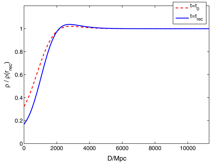
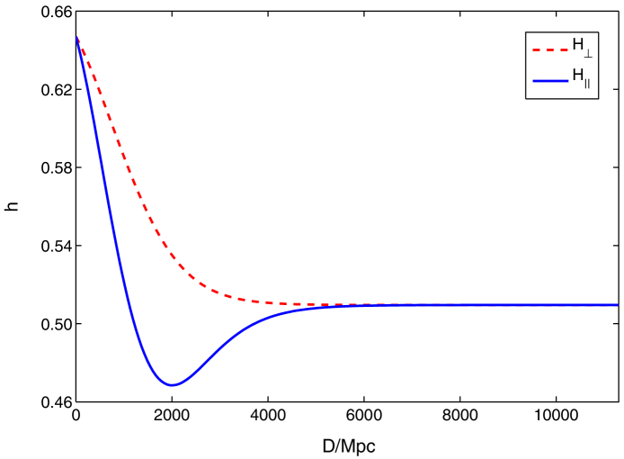
Figure 1: The profile considered in [10]. The subscript $rec$ denotes the value at the recombination, and $H_{\scriptscriptstyle\!/\!/}({\rm or}\ H_{\perp})=100h\rm km/s/Mpc$.

The induced $a_{10}$ is of order $10^{-3}$ or less observed by Cosmic Background Explorer (COBE) [11], so we find that

$$\delta L\hskip 3.50006pt\raisebox{1.72218pt}{$<$}\raisebox{-3.01385pt}{$\sim$}\hskip 3.00003pt15\rm Mpc,$$ (16)

where $\delta L$ is the distance from the observer to the center of the void. This is consist with the result of [10].

5 Summary

In the LTB model, we have derived the analytic formulae for the CMB anisotropy dipole (9) and quadrupole (10), which can be used to rigorously compare consequences of this model with observations of the CMB anisotropy. Moreover, we checked the consistency of our formulae with results of the numerical analysis in [10], and constrained the distance from an observer to the center of the void. One of the advantages in obtaining analytic formulae is that we can identify physical origins of the CMB anisotropy in the LTB model. For example, in the CMB dipole formula (9), we can regard the first term as the initial condition at the last scattering surface, and the second term as the Integrated Sachs-Wolfe effect.

References

- [1] K. Tomita, Astrophys. J. 529, 26 (2000).
- [2] G. Lemaitre, Ann. Soc. Sci. Brux 53, 51 (1933).
- [3] R. C. Tolman, Proc. Nat. Acad. Sci. USA. 20, 169 (1934).
- [4] H. Bondi, Mon. Not. Roy. Astron. Soc. 107, 410 (1947).
- [5] K. Tomita, Astrophys. J. 529, 38 (2000).
- [6] K. Tomita, MNRAS 326, 287 (2001).
- [7] H. Alnes, M. Amarzguioui and Ø. Grøn, Phys. Rev. D73, 083519 (2006).
- [8] M. Kasai, Prog. Theor. Phys. 117, 1067 (2007).
- [9] J. Garca-Bellido and T. Haugbølle, JCAP 0809: 016 (2008).
- [10] H. Alnes and M. Amarzguioui, Phys. Rev. D74, 103520 (2006).
- [11] C. L. Bennett et al., Astrophys. J. 464, L1-L4 (1996).
- [12] K. Tomita, astro-ph/0906.1325.