Electron fraction constraints based on Nuclear Statistical Equilibrium with beta equilibrium

The electron-to-nucleon ratio or electron fraction is a key parameter in many astrophysical studies. Its value is determined by weak-interaction rates that are based on theoretical calculations subject to several nuclear physics uncertainties. Consequently, it is important to have a model independent way of constraining the electron fraction value in different astrophysical environments. Here we show that nuclear statistical equilibrium combined with beta equilibrium can provide such a constraint. We test the validity of this approximation in presupernova models and give lower limits for the electron fraction in type Ia supernova and accretion-induced collapse.

1 Introduction

Weak interactions are known to play a critical role in the structure and evolution of stars and the kind of nucleosynthesis they produce (e.g. Langanke & Martínez-Pinedo, 2003). For nuclei near the valley of beta-stability, the relevant lifetimes of unstable nuclei are well determined in the laboratory. However at the high temperatures and densities found in stars and stellar explosions, nuclei may be produced that are either very proton- or neutron-rich. Usually the rates for weak interactions involving such nuclei are only available from theory. Further, these nuclei exist in a distribution of excited levels, making even a theoretical calculation of their weak lifetimes problematic.

Over the years, different groups have calculated weak-interaction rates for astrophysical applications (for a review see Langanke & Martínez-Pinedo, 2003). In the 1980s Fuller, Fowler, & Newman (Fuller et al., 1980, 1982b, 1982a, 1985, hereafter FFN) calculated rates for electron capture, positron capture, beta decay, and positron emission for astrophysically relevant nuclei. Their tabulations were based on an examination of all available information at that time and became the standard in the field. With the improvement of methods and computers, complete shell-model calculations were performed for $sd$-shell nuclei Oda et al. (1994) and for $pf$-shell nuclei (Langanke & Martínez-Pinedo, 2000, 2001, hereafter LMP). Although these new shell-model rates and the FFN rates agree rather well for $sd$-shell nuclei, there are appreciable difference at higher mass. The electron-capture rates, and to a lesser extent, the beta-decay rates (see Martínez-Pinedo et al., 2000) are smaller than the FFN rates by approximately one order of magnitude.

In this paper we discuss an interesting limiting case that can be used to test existing rate tabulations and their implementation as well as to calculate astrophysical models in regions where rate information may currently be inadequate. Dynamic beta-equilibrium Tsuruta & Cameron (1965); Imshennik et al. (1967); Imshennik & Chechetkin (1971); Cameron (2001); Odrzywolek (2009) occurs when sufficient time elapses at a given temperature and density for the electron mole number, $Y_{e}$, to approach a constant. That is, for an ensemble of nuclei (but not necessarily individual nuclei), electron capture and positron emission occur at a rate balanced by electron emission and positron capture. While physically not the same situation as when neutrino absorption balances neutrino emission (thermal weak equilibrium), the solution to the abundance equations is the same in many of the astrophysical environments of interest, as we will show. Where this approximation holds, a set of nuclear abundances can be obtained, and thus a steady state value for $Y_{e}$, that depends only on nuclear bulk properties (like binding energy and partition function), the temperature, and the density. Similar work was done by Imshennik & Chechetkin (1971), but our results are based on improved nuclear data present a broader overview of the possible astrophysical scenarios where this approximation becomes useful.

There are only a few places in nature where thermal weak equilibrium actually occurs, but they are interesting. Obviously the Big Bang is one, but there the abundances are simple, just neutrons and protons. Dynamic beta-equilibrium exists in neutron stars Baym et al. (1971); Weber (1999) and may occur briefly in the cores of massive stars after silicon burning Aufderheide et al. (1994b, a); Heger et al. (2001a, b). It may also happen in white dwarfs that ignite carbon runaways at very high density Canal et al. (1990). In the latter case, there is thought to exist a critical ignition density above which the reduction in electron density by electron capture more than offsets the rise in thermal pressure due to the burning. Above this density whose exact value depends on composition, initial mass, and accretion rate Canal et al. (1990), it is expected that the white dwarf collapses to a neutron star rather than exploding as a supernova. This scenario is still only theoretical since it was not yet observed. Just short of this critical density, which may be $\sim 8\times 10^{9}$ g cm^-3 Timmes & Woosley (1992); Woosley (1997), the star does explode but ejects neutron-rich isotopes (e.g., ⁴⁸Ca) that are difficult to make elsewhere in nature Woosley (1997). In addition, as the Chandrasekhar mass scales as $M_{\mathrm{Ch}}\propto Y_{e}^{2}$, if a flame reduces the $Y_{e}$ before the star begins to expand vigorously, it will collapse. The race between expansion and electron capture must be determined by hydrodynamical simulations with physical fidelity, preferably in 2D or 3D. Until they are done, it is difficult to make quantitative statements, but it is expected that a 10% change in the terminal value of $Y_{e}$ would cause an approximately 10% change in the terminal density and might affect whether e.g., the critical ignition density for collapse is $8$ or $9\times 10^{9}\mathrm{g/cm}^{3}$ Timmes & Woosley (1992). Instabilities could make the dependence non-linear. Thus it is important to know what the minimum achievable value is for $Y_{e}$ at a given temperature and density.

To proceed, we calculate the electron fraction and the composition assuming thermal weak equilibrium for temperatures and densities that are relevant to various astrophysical environments. Thermal weak equilibrium will only exist at such high temperatures and densities that nuclear statistical equilibrium (NSE) also prevails, and we assume that to be the case. We show that for temperatures, $T\lesssim 10$ GK, thermal weak equilibrium reduces approximately to the dynamic beta-equilibrium of Tsuruta & Cameron (1965). This allows to obtain results that depend only upon binding energies and partition functions, not individual weak interaction rates. At higher temperatures, thermal neutrinos are absorbed with a rate comparable to the electron emission rate. When this happens thermal weak equilibrium and dynamic beta-equilibrium become different. Nevertheless, the equilibrium value of the electron fraction for dynamic beta-equilibrium can still be obtained using a rather simple description of the relevant weak interaction rates.

Our paper is organized as follows. We start with a brief review of NSE, thermal weak equilibrium and dynamic beta-equilibrium in Sect. 2. The results obtained from combining these assumptions are presented in Sect. 3 for broad ranges of temperature and density. In Sect. 4, we discuss the astrophysical implications of our results for presupernova models (Sect. 4.1), proto-neutron star evolution (Sect. 4.2), and accretion-induced collapse and type Ia supernovae (Sect. 4.3). Finally, we conclude in Sect. 5.

2 NSE, thermal weak equilibrium and dynamic beta-equilibrium

At high temperatures ($T>4$ GK $\approx 0.3$ MeV) the photon energy in an astrophysical plasma is high enough to dissociate nuclei into nucleons. At the same time, for densities $\rho\approx 10^{6}-10^{13}\text{g/cm}^{3}$, rapid nuclear reactions lead to the formation of nuclei. An equilibrium is reached between strong and electromagnetic reactions. This is known as the NSE, where the abundances of nuclei follow simply from Saha equation for a given density, temperature, and electron fraction. Although this is well known, we briefly summarize the relevant equations.

When NSE is reached, production and destruction of nuclei occur at the same rate and the chemical potentials of nuclei and nucleons have to satisfy:

$$\mu_{(Z,A)}=Z\,\mu_{p}+(A-Z)\,\mu_{n}\,,$$ (1)

where the chemical potentials include the total mass

$$\mu_{i}=m_{i}c^{2}+kT\eta_{i}+\mu_{c}\,.$$ (2)

Here $\eta_{i}$ is the degeneracy parameter, $k$ the Boltzmann constant, $T$ the temperature, and $\mu_{c}$ the Coulomb contribution to the chemical potential (see appendix in Juodagalvis et al., 2009). The electron chemical potential is given by $\mu_{e}=m_{e}c^{2}+\eta_{e}$.

The abundance $Y_{i}=n_{i}/n$ of isotope $i$ is given by the ratio of its number density $n_{i}$ over the total baryon number density $n$. The number density $n_{i}$ is related to the degeneracy parameter $\eta_{i}$ assuming Maxwell-Boltzmann statistics by:

$$n_{i}=\frac{G_{i}(T)e^{\eta_{i}}}{\Lambda_{i}^{3}}\,,$$ (3)

with the partition function $G_{i}(T)=\sum(2J_{k}+1)e^{-E_{k}/kT}$ and the thermal wavelength $\Lambda_{i}=\sqrt{2\pi\hbar^{2}/m_{i}kT}$. For the partition function we use values calculated by Rauscher (2003).

Protons also follow Maxwell-Boltzmann distributions over the densities of interest, but neutrons become degenerate for $\rho\gtrsim 10^{11}\,\text{g/cm}^{3}$ (the transition from the non-degenerate to degenerate regime of course depends on the temperature). Therefore, we use Fermi-Dirac distributions for nucleons (both neutrons and protons),

$$n_{i}=\frac{8\pi\sqrt{2}}{h^{3}}m_{i}^{3}c^{3}\beta_{i}^{3/2}[\mathcal{F}_{1/2}(\eta_{i},\beta_{i})+\beta_{i}\mathcal{F}_{3/2}(\eta_{i},\beta_{i})]\,,$$ (4)

where $\beta=kT/mc^{2}$ is the so-called relativistic parameter, which is almost zero for the range of temperatures considered here, and $\mathcal{F}_{k}$ are Fermi functions:

$$\mathcal{F}_{k}(\eta,\beta)=\int_{0}^{\infty}\frac{x^{k}(1+\frac{1}{2}\beta x)^{1/2}\text{d}x}{e^{-\eta+x}+1}\,.$$ (5)

The electron mole number is defined as $Y_{e}=n_{e}/n$, with the lepton number density $n_{e}=n_{e^{-}}-n_{e^{+}}$. The electron, $n_{e^{-}}$, and positron, $n_{e^{+}}$, number densities are related to the respective chemical potentials by Eq. (4) with the additional condition $\mu_{e}=\mu_{e^{-}}=-\mu_{e^{+}}$.

Combining Eqs. (1) and (3), the abundance of the nucleus with Z, A is

$$Y(Z,A)=\frac{G_{(Z,A)}}{\rho/m_{u}}\left(\frac{kTAm_{u}}{2\pi\hbar^{2}}\right)^{3/2}e^{(A-Z)\eta_{n}+Z\eta_{p}}e^{B/kT}e^{Z\mu_{c,p}-\mu_{c,(Z,A)}}\,.$$ (6)

Here $\rho$ is the baryon density and $m_{u}$ the atomic mass unit. Note that small corrections (less than $1\%$) arise from using $m_{i}=Am_{u}$ Seitenzahl et al. (2009). To calculate the NSE composition, we take the binding energies, $B=Zm_{p}c^{2}+(A-Z)m_{n}c^{2}-m_{(Z,A)}c^{2}$ from Audi et al. (2003) and supplemented by theoretical values from Möller et al. (1995). In addition, the degeneracy parameters $\eta_{n}$, $\eta_{p}$ are determined by charge neutrality and mass conservation,

$$\sum Z_{i}Y_{i} = Y_{e}\,,$$ (7)

$$\sum A_{i}Y_{i} = 1.$$ (8)

Eqs. (6) - (8) can be solved to obtain $\eta_{n}$, $\eta_{p}$, and $Y(Z,A)$ for given temperature, density and electron fraction.

The electron fraction is generally determined by weak process that are much slower than the strong and electromagnetic nuclear reactions responsible for maintaining NSE. However, if the system remains at a given temperature and density long enough, weak reactions can also reach equilibrium. If the neutrinos produced by the weak interaction do not leave the system, the equilibrium reached is denoted as thermal weak equilibrium. In order to determine the evolution of the system before thermal weak equilibrium is achieved neutrino transport calculations are necessary (see Murphy, 1980). Once, thermal weak equilibrium is achieved, the neutrinos have a Fermi-Dirac spectrum with a temperature, $T$, and neutrino chemical potential $\mu_{\nu}=-\mu_{\bar{\nu}}$. The state of the system is completely determined by the temperature, density and lepton fraction (relative number of electrons and neutrinos).

Once thermal weak equilibrium is reached, the composition does not change unless the temperature or density varies. Therefore, entropy is conserved which implies that $T\mathrm{d}S=\sum_{i}\mu_{i}\mathrm{d}Y_{i}=0$ (see Meyer, 1993, for useful discussion of equilibrium in nucleosynthesis), thus

$$\mu_{\nu}\dot{Y}_{\nu} + \mu_{e}\dot{Y}_{e}+\sum_{i}\mu_{i}\dot{Y}_{i}$$ (9)

$$= (\mu_{e}-\mu_{\nu})\dot{Y}_{e}+(\mu_{p}-\mu_{n})\sum_{i}Z_{i}\dot{Y}_{i}+\mu_{n}\sum_{i}A_{i}\dot{Y}_{i}=0\,,$$

here the right-hand side is obtained from the assumption of NSE and the condition of lepton number conservation that implies, $\dot{Y}_{\nu}=-\dot{Y}_{e}$. The time variation of the abundance of nucleus $i$ is given by $\dot{Y}_{i}$. Using Eqs. (7) and (8) this reduces to

$$(\mu_{e}+\mu_{p}-\mu_{\nu}-\mu_{n})\dot{Y}_{e}=0.$$ (10)

The value of $Y_{e}$ for which equilibrium is attained can be obtained from the thermal weak equilibrium condition

$$\mu_{e}+\mu_{p}=\mu_{\nu}+\mu_{n}.$$ (11)

This implies that the value of the neutrino chemical potential is a function of lepton fraction, temperature, and baryon density. Alternatively, the equilibrium $Y_{e}$ can be obtained from

$$\dot{Y}_{e} = -\sum_{i}(\lambda^{i}_{\text{ec}}+\lambda^{i}_{\beta^{+}}+\lambda^{i}_{\bar{\nu}_{e}}+\lambda^{i}_{\text{in}\beta^{-}})Y_{i}$$ (12)

$$+\sum_{i}(\lambda^{i}_{\text{pc}}+\lambda^{i}_{\beta^{-}}+\lambda^{i}_{\nu_{e}}+\lambda^{i}_{\text{in}\beta^{+}})Y_{i}=0,$$

which requires the knowledge of the weak interaction rates for electron capture (ec), positron emission ($\beta^{+}$), antineutrino absorption ($\bar{\nu}_{e}$), inverse of electron emission (in$\beta^{-}$), positron capture (pc), electron emission ($\beta^{-}$), neutrino absorption ($\nu_{e}$), and inverse of possitron emission (in$\beta^{+}$) for a large ensemble of nuclei. Eqs. (11) and (12) represent equivalent ways of obtaining the steady state value of $Y_{e}$, if entropy is constant. Eq. (11) is certainly advantageous as it depends only on bulk nuclear properties like binding energies and partition functions. However, its applicability is rather limited because at stellar densities below $\sim 10^{11}$ g cm^-3 neutrinos scape and consequently a neutrino chemical potential cannot be defined. In these cases, a dynamical beta-equilibrium can still be achieved and its equilibrium $Y_{e}$ value is given by Eq. (12) suppressing the neutrino absorption rates:

$$\dot{Y}_{e}=-\sum_{i}(\lambda^{i}_{\text{ec}}+\lambda^{i}_{\beta^{+}})Y_{i}+\sum_{i}(\lambda^{i}_{\text{pc}}+\lambda^{i}_{\beta^{-}})Y_{i}=0.$$ (13)

Nevertheless, we will show in the following that Eq. (11) together with the assumption $\mu_{\nu}=0$ provides a very good approximation to the solution of Eq. (13), i.e., thermal weak equilibrium with $\mu_{\nu}=0$ reduces to dynamical beta-equilibrium. In this case the neutrino density depends only on temperature:

$$n_{\nu}=n_{\bar{\nu}} = \frac{1}{2\pi^{2}\hbar^{3}}\int_{0}^{\infty}\frac{p^{2}}{1+\exp(pc/kT)}dp$$ (14)

$$= 7.61\times 10^{27}\left(\frac{T}{\mathrm{GK}}\right)^{3}\ \mathrm{cm}^{-3}\,,$$

with $p$ being the neutrino momentum and $pc$ its energy. At low temperatures the neutrino densities are so small that can be neglected and consequently the condition $\mu_{\nu}=0$ reduces to $n_{\nu}=0$. This is the situation in cold neutron stars where Eq. (11) with $\mu_{\nu}=0$ is commonly used Weber (1999) to determine the composition. However, at higher temperatures the assumption of $\mu_{\nu}=0$ results in neutrino densities comparable to electron densities and consequently thermal weak equilibrium, Eq. (11), and dynamical beta equilibrium, Eq. (13), predict different values of $Y_{e}$. Under these conditions, one has to solve Eq. (13) using a full set of weak interaction rates Odrzywolek (2009).

As discussed in the introduction, the determination of weak-interaction rates on nuclei is a very challenging nuclear structure problem that requires sophisticated many body calculations. Reliable weak-interaction rates are necessary to determine the evolution of the system and to account for the energy loss by neutrinos Odrzywolek (2009). However, in this paper we are not interested in the evolution towards equilibrium, but only in the value of the equilibrium electron fraction for a given temperature and density. Therefore, only a simple description of the weak interaction rates is necessary.

We start considering the case of thermal weak equilibrium under the assumption that $\mu_{\nu}=0$. This has the advantage that we can use Eqs. (11) and (12) to check the validity of our implementation of the weak interaction rates. Once these are validated, we can can easily generalize our approach to the case with neutrinos leaving the system, by setting the neutrino densities to zero. Let us consider a couple of nuclei $(A,Z)$ and $(A,Z-1)$ connected by the weak interactions:

$$e^{-}+(A,Z)\rightleftarrows(A,Z-1)+\nu_{e},$$ (15a)

$$(A,Z)\rightleftarrows(A,Z-1)+e^{+}+\nu_{e},$$ (15b)

$$(A,Z-1)\rightleftarrows(A,Z)+e^{-}+\bar{\nu}_{e},$$ (15c)

$$e^{+}+(A,Z-1)\rightleftarrows(A,Z)+\bar{\nu}_{e}.$$ (15d)

If neutrinos are present, these reactions can operate in both directions. Only the right direction is relevant for cases where neutrinos leave the system. One can approximate these reactions assuming that they occur by a transition from the ground state of the initial nucleus to the ground state of the final nucleus. This is an exact result for neutrons and protons and has been shown to provide a reasonable description of electron capture rates for a broad range of nuclei (see figure 2 of Langanke et al., 2003). Here we generalize this prescription to the other rates in Eq. (15). Our aim is not to obtain accurate weak-interaction rates but an approach that reproduces the balance between forward and reverse reactions once equilibrium is achieved. In this sense our results should not be considered as a substitute to the different tabulations of weak interaction rates available in the literature. We use the following expressions to calculate the weak-interaction rates in Eq. (15):

$$\lambda_{\text{ec}} =C\int_{w_{\text{ec}}}^{\infty}E^{2}(E-Q)^{2} f_{e}(E,\mu_{e})$$ (16a)

$$(1-f_{\nu}(E-Q,\mu_{\nu}))dE,$$

$$\lambda_{\beta^{+}} =C\int_{m_{e}c^{2}}^{-Q}E^{2}(-Q-E)^{2} (1-f_{p}(E,-\mu_{e}))$$ (16b)

$$(1-f_{\nu}(-Q-E,\mu_{\nu}))dE,$$

$$\lambda_{\beta^{-}} =C\int_{m_{e}c^{2}}^{Q}E^{2}(Q-E)^{2} (1-f_{e}(E,\mu_{e}))$$ (16c)

$$(1-f_{\bar{\nu}}(Q-E,-\mu_{\nu}))dE,$$

$$\lambda_{\text{pc}} =C\int_{w_{\text{pc}}}^{\infty}E^{2}(E+Q)^{2} f_{p}(E,-\mu_{e})$$ (16d)

$$(1-f_{\bar{\nu}}(E+Q,-\mu_{\nu}))dE,$$

$$\lambda_{\nu_{e}} =C\int_{w_{\text{ec}}}^{\infty}E^{2}(E-Q)^{2} (1-f_{e}(E,\mu_{e}))$$ (16e)

$$f_{\nu}(E-Q,\mu_{\nu})dE,$$

$$\lambda_{\text{in}\beta^{+}} =C\int_{m_{e}c^{2}}^{-Q}E^{2}(-Q-E)^{2} f_{p}(E,-\mu_{e})f_{\nu}(-Q-E,\mu_{\nu})dE,$$ (16f)

$$\lambda_{\text{in}\beta^{-}} =C\int_{m_{e}c^{2}}^{Q}E^{2}(Q-E)^{2} f_{e}(E,\mu_{e})f_{\bar{\nu}}(Q-E,-\mu_{\nu})dE,$$ (16g)

$$\lambda_{\bar{\nu}_{e}} =C\int_{w_{\text{pc}}}^{\infty}E^{2}(E+Q)^{2} (1-f_{p}(E,-\mu_{e}))$$ (16h)

$$f_{\bar{\nu}}(E+Q,-\mu_{\nu})dE,$$

where the first four equations correspond to the forward direction in Eq. (15) describing the rates for electron capture (ec), positron emission ($\beta^{+}$), electron emission ($\beta^{-}$), and positron capture (pc), respectively. The last four equations describe neutrino absorption ($\nu_{e}$), the inverse of positron emission (in$\beta^{+}$), the inverse of electron emission (in$\beta^{+}$), and antineutrino absorption ($\bar{\nu}_{e}$). $Q$ is the transition Q value, i.e. $Q=M(A,Z-1)c^{2}-M(A,Z)c^{2}$, that is positive for neutron-rich nuclei and protons. $M(A,Z)$ is the nuclear mass. The quantity $C$ is given by

$$C=\frac{B\ln 2}{K(m_{e}c^{2})^{5}},$$ (17)

with $K=6144$ s (Hardy & Towner, 2009) and $B$ the nuclear matrix element. We use the value $B=1+3g_{A}^{2}=5.76$ for nucleons and $B=4.6$ for nuclei (Langanke et al., 2003). We have checked that our results are not sensitive to 20% variations of this value. $f$ is the Fermi-Dirac distribution

$$f(E,\mu)=\frac{1}{1+\exp[(E-\mu)/kT]}\,.$$ (18)

The quantity $w_{\text{ec}}=\max(m_{e}c^{2},Q)$ is the threshold energy for electron capture, and $w_{\text{pc}}=\max(m_{e}c^{2},-Q)$ for positron capture rate. The integral in Eqs. (16b) and (16f) are defined only for $-Q>m_{e}c^{2}$. Similarly, the integrals in Eqs. (16c) and (16g) are defined only for $Q>m_{e}c^{2}$.

The value of the equilibrium electron fraction agrees up to 3 significant figures when we solve Eq. (11) or Eq. (12). This justifies our simple scheme, Eq. (16), for calculating the weak interaction rates.

Dynamic beta-equilibrium, Eq. (13), can be obtained from the rates in Eqs. (16) setting the neutrino distributions to zero. The equilibrium electron fraction in dynamic beta-equilibrium is typically smaller than the one calculated in thermal weak equilibrium. As in the latter, neutrino absorption results in an increase of the electron fraction.

3 Results

We solve the NSE equations (Eqs. (6)-(8)) under the constraint of thermal weak equilibrium, Eq. (11), assuming $\mu_{\nu}=0$ for temperatures from 5 to 150 GK ($0.43-13\,\text{MeV}$) and densities in the range $10^{6}-10^{12}\,\text{g}/\text{cm}^{3}$. This results in the equilibrium electron fraction shown in Fig. 1 and in the composition shown in Figs. 4,  5, and  6. Because only small changes are expected at high temperatures, we plot all quantities only over a smaller temperature range. The whole data table is available on request.

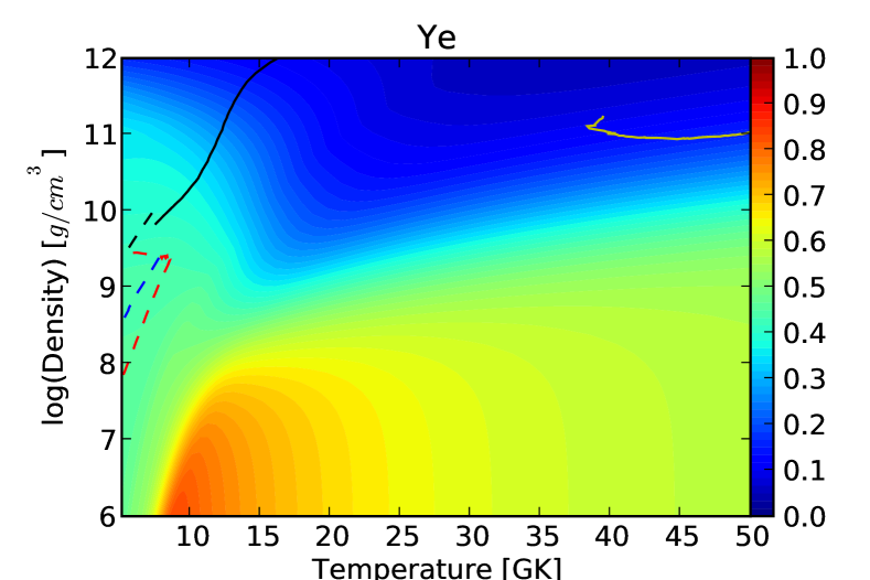
Figure 1: The electron fraction for NSE with thermal weak equilibrium is shown by color contours for a range of densities and temperatures where NSE can be applied and which are relevant in different astrophysical scenarios. The solid black line shows the core-collapse trajectory for a 15 $M_{\odot}$ (A. Marek priv. com.); the dashed lines represent the presupernova evolution of a 15 $M_{\odot}$ (black) and 25 $M_{\odot}$ (blue) stars; the red dashed lines represent a type Ia trajectory (F. Röpke priv. com.); and the solid yellow lines correspond to the evolution of the proto-neutron star surface. Not all these scenarios will reach beta equilibrium and their electron fraction can therefore be different to the one shown here.

In Fig. 1 the color contours show the electron fraction assuming thermal weak equilibrium and the lines represent trajectories (density and temperature evolution) of various astrophysical scenarios: presupernova, core collapse, proto-neutron star surface, and type Ia supernovae. The collapse trajectory (A. Marek priv. com.) of a 15 $M_{\odot}$ star based on the presupernova models of Woosley et al. (2002) is shown by the solid black line. When the inner core of a massive star collapses the evolution is much faster than weak reactions, therefore beta equilibrium is not achieved. Once densities above $10^{11}$ g cm^-3 are reached neutrinos begin to be trapped and the assumption of $\mu_{\nu}=0$ is not valid any more. Therefore, the equilibrium $Y_{e}$ differs from the value obtained in detailed hydrodynamical simulations with neutrino transport. However, we include this trajectory in our figure for completeness, to have an idea of the range of temperatures and densities we are studying. Presupernova trajectories for 15 $M_{\odot}$ and 25 $M_{\odot}$ stars Woosley et al. (2002) are shown by the dashed lines. This is discussed in detail in Sect. 4.1. The solid yellow line in the high temperature region represents the evolution of the hot proto-neutron star surface, where both thermal weak equilibrium and NSE are fulfilled (Sect. 4.2). And the red dashed line represents a trajectory of a type Ia supernova (F. Röpke priv. com.), where the evolution normally proceeds much faster than the weak interaction timescale and consequently no equilibrium is achieved (Sect. 4.3).

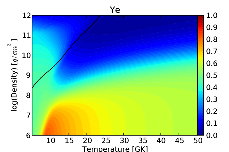
Figure 2: The electron fraction for NSE with dynamic beta-equilibrium is shown by color contours for the same range as in Fig. 1. The black line represent the region where $\lambda_{\bar{\nu}_{e}}=\lambda_{\beta^{-}}$.

For completeness we show in Fig. 2 the electron fraction obtained in NSE assuming dynamic beta-equilibrium, Eq. (13), for the same temperatures and densities as shown in Fig. 1. As discussed in Sect. 2, we expect that dynamic beta-equilibrium and thermal weak equilibrium with $\mu_{\nu}=0$ give similar electron fraction whenever the absorption of thermal neutrinos is negligible. This occurs on the left side of the solid line shown in Fig. 2. This line marks the conditions for which the antineutrino absorption would become equal to beta decay if neutrinos did not escape. At high temperatures the results for both equilibria are not so different because the composition is dominated by neutrons and protons and moreover positron captures also become important. In fact, at low densities (below the curve marked as $\eta_{e}=0$ in Fig. 3) one has that $\mu_{e}\approx\mu_{e^{+}}\approx 0$ implying that the contributions of electrons/positrons and antineutrinos/neutrinos are similar. This explains why both equilibria lead to same electron fraction for Big Bang conditions. The biggest differences between both approaches appear in the region where the composition changes from heavy nuclei to nucleons (Fig. 3). Moreover, it is in this region where the electron fraction drops more abruptly and consequently its value becomes rather sensitive to the equilibrium approach used.

Although solution of the full equations gives the value of the equilibrium electron fraction, some simple approximations help to understand the results. We divide the $\rho-T$ plane in different temperature and density ranges to explain the behaviour of the electron fraction. These ranges are shown in Fig. 3. The two horizontal lines correspond to electron and neutron degeneracy equal zero. We consider densities below the line of $\eta_{e}=0$ to be low and above the line of $\eta_{n}=0$ to be high. The temperatures are considered to be low when heavy nuclei or alpha particles are present, which in the figure correspond to the regions labeled as $X_{heavy}>0.5$ and $X_{a}>0.5$, respectively.

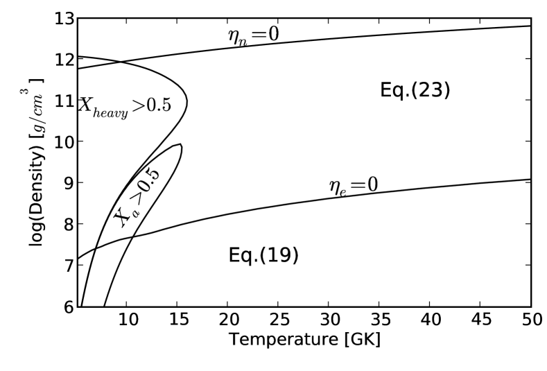
Figure 3: Lines limit the regions where different approximations for $Y_{e}$ can be used. Horizontal lines indicate where the degeneracy of electrons ($\eta_{e}$) and neutrons ($\eta_{n}$) is zero. The regions where nuclei and alpha particles dominate the composition are at low temperatures.

In NSE at high temperature ($T\gtrsim 15$ GK) one can assume that only nucleons are present because all nuclei are dissociated, thus $Y_{e}=Y_{p}$ and $Y_{n}=1-Y_{e}$. For low densities conditions are similar to the Big Bang, where the composition consists mainly of non-degenerate neutrons, protons, and electrons. Therefore, we have $\mu_{e}=0$ and $\mu_{n}\approx\mu_{p}$ that together with Eq. (3) give:

$$Y_{e}=\frac{1}{1+e^{-\Delta/kT}}\,,$$ (19)

where $\Delta=m_{n}-m_{p}=1.293$ MeV. Under these conditions $Y_{e}$ can reach rather high values when the temperature becomes smaller than $\Delta$. At higher densities ($\rho\gtrsim 10^{8}-10^{9}\,\mathrm{g/cm}^{3}$), electrons become degenerate and this approximation is not valid anymore. This happens when the density is above:

$$\rho\geq 1.132\cdot 10^{7}\frac{(kT)^{3/2}}{Y_{e}}(0.6773+2.256\,kT)\,,$$ (20)

which corresponds to Eq. (4) assuming $\eta_{e}\approx 0$ and using the values from Bludman & van Riper (1977) for the Fermi functions ($\mathcal{F}_{1/2}(\eta=0)=0.6773$ and $\mathcal{F}_{3/2}(\eta=0)=1.153$). This line is shown in Fig. 3 labeled as $\eta_{e}=0$.

For densities above the line given by Eq. (20) the electron fraction can be estimated by taking into account that the electron number density is approximately given by:

$$n_{e}=8\pi\left(\frac{kT}{hc}\right)^{3}\frac{1}{3}\eta_{e}^{3}\,.$$ (21)

From this equation we get directly $\eta_{e}$. If we assume that the nucleons follow Maxwell-Boltzmann distributions (Eq. (3)), their chemical potentials are:

$$\mu_{n(p)}=m_{n(p)}c^{2}+kT\text{ln}\left(\frac{n_{n(p)}\Lambda_{n(p)}^{3}}{G}\right)\,.$$ (22)

Inserting all this in the beta equilibrium equation ($\mu_{n}=\mu_{p}+\mu_{e}$) we obtain a non-linear equation for the electron fraction:

$$\Delta-m_{e}c^{2}+kT\text{ln}\left(\left(\frac{m_{p}}{m_{n}}\right)^{3/2}\frac{1-Y_{e}}{Y_{e}}\right)-\left(\frac{3Y_{e}\rho}{8\pi m_{u}}\right)^{1/3}\frac{hc}{kT}=0\,.$$ (23)

This can be solved numerically using as guess value the $Y_{e}$ of Eq. (19). At high density, low $Y_{e}$ (more neutron-rich material) is expected from Eq. (23). The last term in Eq. (23) increases as the density increases, unless $Y_{e}$ decreases. Moreover, a reduction of $Y_{e}$ leads to an increase of the third term, which has opposite sign to the term containing the density. The exact solution, shown in Fig. 1, demonstrates the neutron richness of the matter at high densities.

For low temperatures ($T\lesssim 15$ GK) the situation is more complicated because of the presence of bound nuclei. We estimate the densities and temperatures at which nuclei dominate the composition following the derivation of Hoyle & Fowler (1960). This leads to nuclei (represented by $\,{}^{56}$Fe) corresponding to half of the mass at:

$$\log\rho=11.62+1.5\log T_{9}-\frac{39.17}{T_{9}}.$$ (24)

In a similar way, taking mass fraction ($X_{i}=A_{i}Y_{i}$) of alpha particles $X_{\alpha}=0.5$, alpha particles represent half of the mass, for which one has:

$$\log\rho=29.68+4.5\log T_{9}+\log\frac{X_{\alpha}}{X_{p}^{2}X_{n}^{2}}-\frac{142.62}{T_{9}}\,,$$ (25)

where $X_{\alpha}$, $X_{n}$, and $X_{p}$ are the alpha, neutron, and proton mass fractions, respectively, which are obtained from mass and charge conservation:

$$1 = X_{\alpha}+X_{p}+X_{n}\,,$$ (26)

$$Y_{e} = \frac{1}{2}X_{\alpha}+X_{p}\,.$$ (27)

At low densities, between the two lines given by Eqs. (24) and (25), there are mainly alpha particles, therefore $Y_{e}=0.5$. Above the line given by Eq. (24), the composition is more complicated due to the presence of different nuclei. For high density the nuclei become neutron rich. We can delimit the region where heavy nuclei are present using simple approximations, as described before. However, the detail composition and thus the electron fraction in this region can only be obtained by numerically solving NSE equations under the assumption of thermal weak equilibrium or dynamic beta-equilibrium, as described in Sect. 2.

The mass fraction of alpha-particles is shown in Fig. 4. Alpha-particles appear mostly at low density and temperature, between the region where nucleons dominate the composition (high temperature) and the region where heavier nuclei are formed from the alpha particles. Notice that the formation alpha particle leads to a change in the behaviour of $Y_{e}$ at low densities (Fig. 1). The mass fractions of heavy nuclei ($A>4$) are shown in the panel (a) of Fig. 5, they dominate the composition at low temperatures and high densities. Figure 5 shows the average mass, proton and neutron numbers of the nuclei in panels (b), (c), and (d) respectively. In addition we find that the abundances of light nuclei (A $<4$) are significant at high temperatures and relative high densities, as shown in Fig. 6. Such conditions are found in the outer layer of the proto-neutron star which is still hot as shown by the trajectory (yellow line) in Fig. 1.

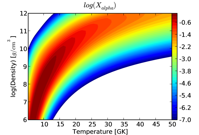
Figure 4: Mass fraction of alpha particles for the same temperature and density range as in Fig. 1. In the white regions the mass fraction of alpha particles is negligible.

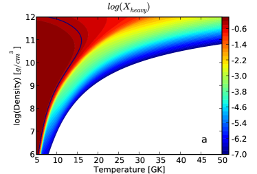
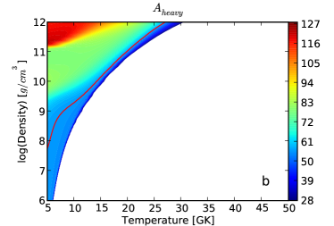
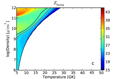
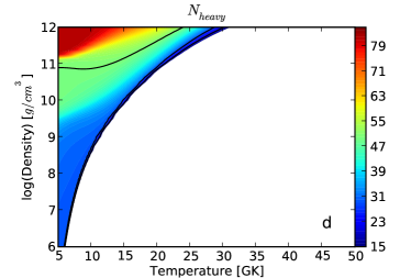
Figure 5: The panel (a) shows the mass fraction of heavy nuclei (A $>$ 4), in the white region no heavy nuclei are present. The other panels give the average mass (b), atomic (c), and neutron (d) numbers. The blue line in the mass fraction plot marks the contour where heavy nuclei are half of the mass. In the average number plots, the black lines correspond to magic numbers and the red ones to $\,{}^{56}$Fe.

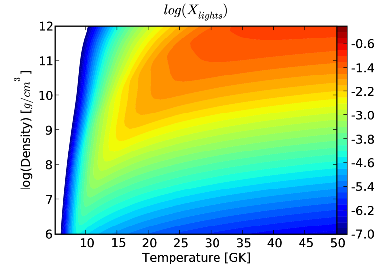
Figure 6: Mass fraction of light nuclei (A$<$4).

4 Discussion and astrophysical implications

There are several astrophysical environments where our results are interesting (Fig. 1). These are situations where sufficient time elapses at high temperature for NSE to prevail and for weak interactions to approach equilibrium. Even when equilibrium is not fully achieved, our results give an interesting lower bound on $Y_{e}$ in cases where electron capture is dominant.

4.1 Presupernova evolution

We investigate here two presupernova models that were already studied in detail in the frame of weak interactions by Heger et al. (2001a, b). Fig. 7 shows the results for the 15 $M_{\odot}$ star in the left column and for the 25 $M_{\odot}$ star in the right one. All results are plotted versus time before collapse which is at time zero. The dotted lines are the $Y_{e}$ of the old models of Woosley & Weaver (1995) (WW). These models were computed with electron-capture rates of Fuller et al. (1980) (FFN) and beta-decay rates of Hansen (1968); Mazurek et al. (1974). The dashed lines were obtained when using the weak-interaction rates of Langanke & Martínez-Pinedo (2001) (LMP) in the calculation of the presupernova models. These two results were already presented in Heger et al. (2001a, b), where they discuss that differences in the electron fraction are mainly due to discrepancies between the old beta decay rates and the new ones. The bottom panels in Fig. 7 show the electron-capture and beta-decay rates as calculated by Langanke & Martínez-Pinedo (2001) and used for the presupernova models presented in Heger et al. (2001a, b).

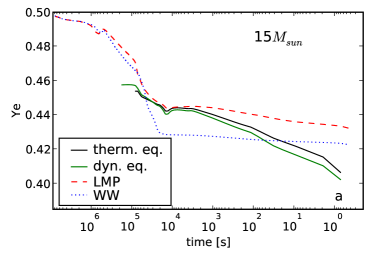
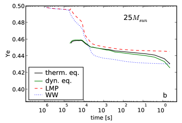
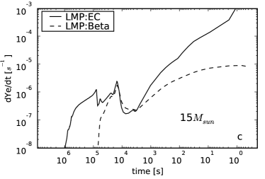
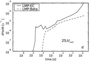
Figure 7: The electron fraction (upper plots), the electron-capture, and beta-decay rates (bottom plots) as a function of time till collapse are shown for two presupernova models: 15 $M_{\odot}$ (left) and 25 $M_{\odot}$ (right). In the electron fraction plots the dotted lines (blue) and dashed lines (red) were already shown by Heger et al. (2001a) and correspond to the old models of Woosley & Weaver (1995) and to the new ones of Heger et al. (2001b), respectively. Here we have added the solid lines, which results from assuming NSE and thermal weak equilibrium (solid black line) or dynamic beta-equilibrium (solid green line).

Before silicon burning, the evolution of the electron fraction is very similar for WW and LMP because electron captures dominate over beta decays (see bottom panels in Fig. 7) and these rates are similar for FFN and LMP. In this first phase when $Y_{e}$ starts to decrease from the starting value of 0.5, the temperature is too low and the assumption of NSE is not valid and there are no values for the equilibrium electron fraction.

During silicon shell burning the electron fraction continues dropping and beta decay becomes important and comparable to electron capture. For the 15 $M_{\odot}$ star both rates are equal and a dynamic beta-equilibrium is reached Aufderheide et al. (1994a); Heger et al. (2001b). After silicon burning the electron fraction stays almost constant although electron captures become dominant over beta decays because the dynamical evolution is faster than the capture rates. Therefore, as it was pointed out by Heger et al. (2001b), the final electron fraction is set before the core begins its final contraction. The most important period for determining the core structure is thus the silicon shell burning phase.

We use the density and temperature evolutions shown in Fig. 1 for the presupernova models of Woosley & Weaver (1995) and calculate the equilibrium electron fraction. This $Y_{e}$ correspond to the solid lines in the upper panels of Fig. 7. Notice that there are two solid lines, the black one results from the assumption of thermal weak equilibrium, Eq. (11), while the green one is obtained under the assumption of dynamic beta-equilibrium, Eq. (13). The resulting $Y_{e}$ values are almost identical. For the 15 M_⊙ star, where dynamic beta-equilibrium is achieved in the simulation (see lower right panel of Fig. 7), all the $Y_{e}$ values are almost identical for times around $10^{4}$ s. For the 25 M_⊙ star, dynamic beta-equilibrium is never reached and consequently our equilibrium $Y_{e}$ is slightly smaller.

Our equilibrium electron fraction represents a static equilibrium and is obtained independently of the weak-interaction rates. Such an equilibrium is reached if the temperature and density are kept constant long enough. There are two points that a set of weak-interaction rates has to fulfil to be used in presupernova models: 1) if dynamic beta-equilibrium is reached, the electron fraction should be very similar to our equilibrium electron fraction; 2) the electron fraction in the presupernova models can not drop below the equilibrium value we calculate. The older presupernova models of Woosley & Weaver (1995) do not fulfil these two constraints. Aufderheide et al. (1994a); Heger et al. (2001b) suggested that older models needed to be recomputed with consistent set of weak-interaction rates. The new results Heger et al. (2001b) based on better determination of the rates satisfy the two constraints. This test should also apply to future compilations of weak-interaction rates and their implementation in presupernova simulations.

4.2 Proto-neutron star

Iron core collapse marks the end of the presupernova phase. When the collapse starts the dynamical evolution is very fast compared to the weak interaction timescale, thus the assumption of equilibrium is not valid. But when collapse continues, neutrinos are trapped due to the increasingly higher central densities, and thermal weak equilibrium can be reached again. However, neutrinos are trapped and their chemical potentials are not negligible anymore ($\mu_{\nu}\neq 0$). Therefore, our results give just a rough estimation of the electron fraction during collapse, but nevertheless are useful to have an idea of the composition in the collapsing material. In Fig. 1 the trajectory of the collapse is in a region where almost only heavy neutron-rich nuclei and neutrons are present (Fig. 5). The amount of alpha particles (Fig. 4) and light nuclei (Fig. 6) is negligible.

When central density gets above the density of nuclear matter, collapse stops and falling matter bounces back leading to the formation of a shock. The way this shock propagates through the outer layers of the star in a supernova explosion is still a problem under discussion Janka et al. (2007). But it is known that a compact object forms in the center and cools by neutrino emission. Neutrinos start to decouple from matter at the neutrinosphere that is placed in the outer layers of the newly born proto-neutron star. In this region we assume still that $\mu_{\nu}\approx 0$. Also NSE is satisfied because the temperatures are high enough, $T\approx 50\cdot 10^{9}$ K. We compare our equilibrium electron fraction with the one obtained in hydrodynamical simulations of core-collapse supernovae Arcones et al. (2007). Figure 8 shows the post-bounce evolution of the electron fraction. The dashed line is the result of the hydrodynamical simulation of Arcones et al. (2007) for their standard case (M15l1r1), and solid line is the equilibrium electron fraction computed for same density and temperature evolution as for the dashed line. There is a clear discrepancy between the two electron fractions that increases with time. This disagreement comes from the difference in the composition (see Fig. 4 in Arcones et al., 2008). The equations of state that are generally used in supernova simulations include only nucleons, alpha particles, and a representative heavy nucleus. In our calculation of NSE with beta equilibrium, we take into account all nuclei. Figure 6 shows that the abundances of light elements ($A<4$) are not negligible in the outer layers of the proto-neutron star. Similar results are found with other EoS, for example Horowitz & Schwenk (2006) and Typel et al. (2010). Light nuclei are formed at expenses of the few free protons. This produces also a reduction of the antineutrino absorption and electron captures, which leads to an increase of the electron fraction compared to the case where only neutrons and protons are present (see Eq. (12)).

These light nuclei have an impact on the properties of neutrinos emitted during the first seconds after bounce (Arcones et al. (2008)). Sumiyoshi & Röpke (2008) have also pointed out the influence of the light elements during the post-bounce evolution. These calculations were both done in a post-processing step, therefore the real effect of light elements in the dynamics of the supernova evolution is still an open issue that has to be studied in detail by using an equation of state that includes light nuclei in supernova simulations.

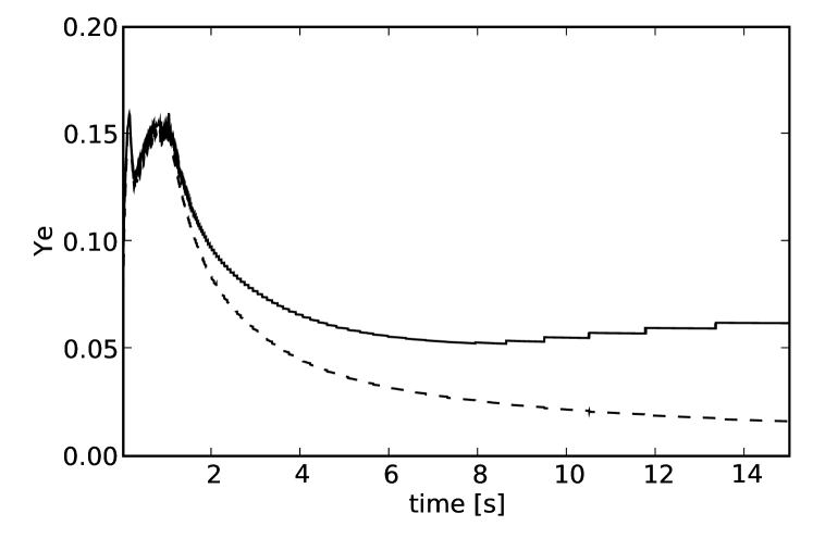
Figure 8: The evolution of the electron fraction at the proto-neutron star surface is shown. The solid line is obtained by assuming NSE and thermal weak equilibrium, while the dashed line results from the hydrodynamical simulation of the supernova explosion and the subsequent neutrino-driven wind of Arcones et al. (2007).

4.3 Type Ia supernovae and Accretion-induced collapse

Other astrophysical scenarios where the electron fraction plays an important role involve the evolution of white dwarfs in binary systems. A white dwarf accreting up to the Chandrasekhar limit can have two possible outcomes. If the density and temperature become sufficiently high to ignite explosive nuclear burning, then the white dwarf may become a type Ia supernova. But it could also happen that electron capture in the ash reduces central temperature and pressure, and the white dwarf instead collapses to a neutron star. This latter outcome is known as “accretion-induced collapse”, or AIC Canal et al. (1990); Woosley & Baron (1992); Fryer et al. (1999). Which outcome occurs depends on the ignition density which is in turn determined by the initial white dwarf properties (mass, composition, and temperature) and on the accretion rate Canal et al. (1990).

The outcome also depends on the weak interaction rates employed in the study and the multi-dimensional character of the explosion. Burning raises the temperature at constant pressure and, if $Y_{e}$ is constant, that must reduce the density. The density inversion behind the flame drives a Rayleigh-Taylor instability that greatly enhances the advance of the burning front. However, since the pressure is mostly due to relativistic electrons, a decrease in $Y_{e}$ due to electron capture in the ash means that the post-burning density will be larger (since pressure depends on the product $\rho Y_{e}$). If $Y_{e}$ decreases sufficiently, the density beneath the flame may even rise, thus suppressing the Rayleigh-Taylor instability (see Sect. 4 in Timmes & Woosley, 1992). If $Y_{e}$ decreases in a sufficient fraction of the white dwarf before the (now slowly moving) flame makes its way out to regions where the density is lower and electron capture is reduced, the white dwarf collapses. At densities approaching 10¹⁰ g cm^-3 electron capture is so efficient that it would drive $Y_{e}$ to very low values were it not for the inhibiting effect of beta-decay. Yet there are, so far, no accurate calculations of beta-decay rates for $Y_{e}$ below about 0.41. Having a reliable lower bound to $Y_{e}$ at a given density will thus be useful in future simulations.

During this phase of the white dwarf evolution, temperatures are high and densities relatively low. Consequently, the produced neutrinos escape. Under such conditions, the lower limit of the electron fraction is thus obtained from dynamic beta-equilibrium, Eq. (13). If thermal weak equilibrium were assumed, electron captures would compete with antineutrino absorptions instead of $\beta^{-}$ decay, as expected when neutrinos escape. Figure 9 shows the dynamic beta-equilibrium electron fraction for the range of temperatures and densities relevant for AIC and type Ia supernovae. In Tab. 1 some numerical values of the $Y_{e}$ in the figure are given (a complete table is available on request).

The behaviour of the electron fraction is very different at high and low temperatures (Fig. 9). At low temperatures the electron fraction decreases continuously with density. While a high temperatures ($T\gtrsim 12$ GK) first decreases and then increases. This seems unintuitive but it can be understood considering the change in composition. At low densities the composition is neutrons, protons, and alpha-particles. With increasing density heavy nuclei are present and their $\beta^{-}$ decay produces an increase of $Y_{e}$. At even higher densities, electron capture dominates and $Y_{e}$ decreases again.

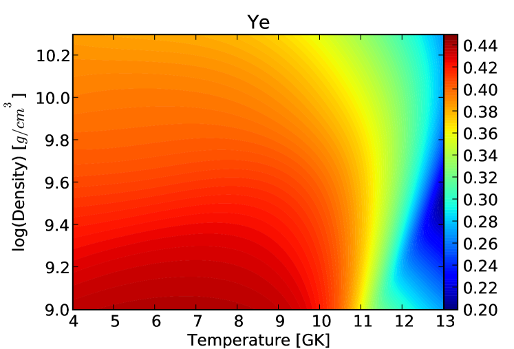
Figure 9: The dynamic beta-equilibrium electron fraction (Eq. (13)) is shown for the range of temperatures and densities relevant in type Ia supernovae and AICs. In Table 1 numerical values of the equilibrium electron fraction are given.

$\rho_{9}=$	1.02	2.11	3.03	4.05	5.04	7.24	9.00	14.96	20.00
$T_{9}=$ 13.03	0.269	0.224	0.202	0.207	0.229	0.256	0.265	0.270	0.266
$T_{9}=$ 12.02	0.299	0.282	0.307	0.319	0.324	0.326	0.325	0.314	0.305
$T_{9}=$ 11.09	0.351	0.371	0.373	0.371	0.369	0.362	0.357	0.342	0.332
$T_{9}=$ 10.03	0.419	0.410	0.405	0.399	0.394	0.385	0.379	0.365	0.355
$T_{9}=$ 9.075	0.434	0.423	0.416	0.409	0.404	0.395	0.390	0.377	0.369
$T_{9}=$ 8.044	0.437	0.428	0.420	0.413	0.407	0.399	0.395	0.385	0.377
$T_{9}=$ 7.058	0.438	0.428	0.420	0.412	0.406	0.400	0.396	0.388	0.381
$T_{9}=$ 6.010	0.438	0.427	0.418	0.410	0.405	0.399	0.397	0.389	0.383

Table 1: Dynamic beta-equilibrium electron fraction for density values given in the first row and temperature values in the first column. The temperature is in units of $10^{9}$ K and the density in $10^{9}$ g cm^-3. These temperature and density intervals correspond to the Fig. 9.

Finally, we notice that the electron fraction and thus weak-interaction rates are important for determining the composition of the ejecta in typical type Ia supernova. In these events the electron captures are very important during the flame propagation because they lead to a reduction of the electron fraction which is the parameter that controls the isotopic composition of the ejecta.

5 Conclusions

Weak-interaction rates determine the evolution of the electron fraction, which is a key parameter affecting the composition and dynamics of stars in the late stages of stellar evolution and supernovae. Here we have presented an interesting limiting case that can be used to test the implementation of theoretical weak-interaction rates in stellar evolution simulations and to place lower bounds on the $Y_{e}$ in the explosion of white dwarfs. Our results depend only on chemical potentials and therefore are independent of the weak-interaction rates.

These equilibrium electron fractions can be compared to those found in presupernova models, where weak-interaction rates play an important role Heger et al. (2001a). The presupernova phase precedes the collapse of massive stars, therefore temperatures get high enough that NSE is reached, but the dynamical evolution is too fast in most cases for beta equilibrium to be achieved. We find a lower limit for electron fraction and show that the $Y_{e}$ in the old presupernova models of Woosley & Weaver (1995) drops below it. In these presupernova models beta decay rates of Hansen (1968); Mazurek et al. (1974) were used. These rates are too low compared to FFN and LMP. Similar models calculated using more recent weak rates Heger et al. (2001b) lead to an electron fraction that stays always above or equal to our lower limit. Moreover, for the 15 $M_{\odot}$ model where the rates predict dynamic beta-equilibrium, we find that their electron fraction agrees with the equilibrium value of our calculations.

The accretion onto white dwarfs approaching the Chandrasekhar mass could lead to type Ia supernovae or to AIC. The final outcome depends on the competition between explosive ignition and electron captures Canal et al. (1990). Therefore, the electron fraction is a key parameter. In this environment densities and temperatures drive the NSE composition towards neutron-rich nuclei whose weak-interaction rates are not yet known from theoretical models. Here we give a reliable lower limit for $Y_{e}$, that can be used in simulations (data are available on request).

In addition, our calculations show that the amount of light elements ($A<4$) in the outer layer of the proto-neutron star is not negligible. After supernova explosion a hot proto-neutron star is born and cools emitting neutrinos. The surface of the proto-neutron star, where neutrinos decouple from matter, is hot enough to assume NSE and its evolution is rather slow, thus beta equilibrium is also satisfied. Changes in the composition of this region have an impact on neutrino properties that could affect the nucleosynthesis Arcones et al. (2008) and the explosion Sumiyoshi & Röpke (2008).