Color-charge separation in trapped SU(3) fermionic atoms

Abstract

Cold fermionic atoms with three different hyperfine states with SU(3) symmetry confined in one-dimensional optical lattices show color-charge separation, generalizing the conventional spin charge separation for interacting SU(2) fermions in one dimension. Through time-dependent DMRG simulations, we explore the features of this phenomenon for a generalized SU(3) Hubbard Hamiltonian. In our numerical simulations of finite size systems, we observe different velocities of the charge and color degrees of freedom when a Gaussian wave packet or a charge (color) density response to a local perturbation is evolved. The differences between attractive and repulsive interactions are explored and we note that neither a small anisotropy of the interaction, breaking the SU(3) symmetry, nor the filling impedes the basic observation of these effects.

One of the most intriguing effects of strong correlations in low-dimensional systems is the separation of charge and spin degrees of freedom. As a generic phenomenon, a quantum particle carrying spin and charge converts in separate spin (spinon) and charge (holon) excitations with generally different velocities. On a microscopic bare level, there are rare examples where this process can be exactly studied in terms of explicit ($n$ species) spinon and holon wave functions, as is the case for the Kuramoto-Yokoyama model PhysRevLett.67.1338 ; PhysRevB.65.195112 ; PhysRevB.74.024423 ; PhysRevB.75.024405 . However, on a low-energy effective field theory level, spin-charge separation (SCS) explicitly manifests itself in all generic one-dimensional interacting systems belonging to the Luttinger liquid universality class, where spinons and holons are described by independent collective density-type excitations Giamarchi_BOOK2004 . In spite of several attempts, the direct experimental observation of SCS has proved elusive Bockrath_Cobden_Lu_Rinzler_Smalley_Balents_McEuen_N1999 ; Segovia_Purdie_Hengsberger_Baer_N1999 ; Losio_Altmann_Kirakosian_Lin_Petrovykh_Himpsel_PRL2001 ; Lorenz_Hofmann_Gruninger_Freimuth_Uhrig_Dumm_Dressel_N2002 . So far, the best experimental evidence is provided by tunneling between quantum wires where interference effects relate to the existence of excitations with different velocities Auslaender_Steinberg_Yacoby_Tserkovnyak_Halperin_Baldwin_Pfeiffer_West_S2005 .

Since recently, one possible avenue for the observation and exploration of SCS are ultracold Bose or Fermi gases confined in optical lattices that have become an important instrument for investigating the physics of strong correlations. The great advantage of these systems is that the interaction parameters and dimensionality can be tuned with very high precision and control by means of an atomic Feshbach resonance or by changing the depth of the wells in an optical lattice Lewenstein_Sanpera_Ahufinger_Damski_Sen_Sen_AIP2007 . One of the first achievements in this subject is the experimental observation of a superfluid to Mott insulator transition in a three-dimensional optical lattice with bosonic ⁸⁷Rb atoms Greiner_Mandel_Esslinger_Hansch_Bloch_N2002 . Interesting experimental results have also been obtained for fermions, like the study of the molecule formation through the Feshbach resonance Stoferle_Moritz_Gunter_Kohl_Esslinger_PRL2006 , the experimental observation of fermionic superfluidityChin_Miller_Liu_Stan_Setiawan_Sanner_Xu_Ketterle_N2006 , and the observation of a Mott insulator in an optical lattice Jordens_Strohmaier_Gunter_Moritz_Esslinger_N2008 . Several theoretical works have addressed the possibility of observing SCS in cold-fermionic gases Kollath_Schollwock_Zwerger_PRL2005 ; Schmitteckert_Schneider_HPC2006 ; Kollath_Schollwock_NJP2006 ; Schmitteckert_HPC2007 ; Ulbricht_Schmitteckert_EPL2009 ; Ulbricht_Schmitteckert_EPL2010 and in cold-bosonic gases Kleine_Kollath_McCulloch_Giamarchi_Schollwock_PRA2008 with two internal degrees of freedom. Thanks to the special properties of cold atomic systems these theoretical proposals could address previously unexplored features of SCS, like the problem of the breaking of SU(2) symmetry and SCS at high energies. In particular, higher spin fermions can be directly studied with cold atoms in more than two hyperfine states. This kind of systems could give rise to new phases in optical lattices due to the emergence of triplets and quartets (three or four fermion bound states), and other phenomena  Honerkamp_Hofstetter_PRL2004 ; Wu_PRL2005 ; Lecheminant_Boulat_Azaria_PRL2005 ; Kamei_Miyake_JPSJ2005 ; Rapp_Zarand_Honerkamp_Hofstetter_PRL2007 ; gorshkov ; PhysRevB.80.180420 . At least two alkali atoms ⁶Li and ⁴⁰K seem to be possible candidates for the experimental realization of an SU(3) fermionic lattice with attractive interactions Rapp_Zarand_Honerkamp_Hofstetter_PRL2007 . In the case of ⁶Li the scattering lengths for the three possible channels of the three lowest lying hyperfine levels ($\left|F,m\right\rangle=\left|1/2,1/2\right>$, $\left|1/2,-1/2\right>$, and $\left|3/2,-3/2\right>$) at large magnetic fields become similar for the three of them $a_{s}\approx-2500a_{0}$ Bartenstein_Altmeyer_Riedl_Geursen_Jochim_Chin_Denschlag_Grimm_Simoni_Tiesinga_Williams_Julienne_PRL2005 . Moreover, the realization of a stable and balanced three-component Fermi gas has been recently reported to potentially accomplish both an attractive and repulsive regime with approximate SU(3) symmetry Ottenstein_Lompe_Kohnen_Wenz_Jochim_PRL2008 ; PhysRevLett.102.165302 . The scattering lengths of the different channels for the three lowest hyperfine states of ⁴⁰K near the Feshbach resonance was also measured and the possibility of trapping them optically was demonstrated Regal_Thesis2005 .

It is the purpose of this work to use time-dependent Density Matrix Renormalization Group (td-DMRG) White_PRL1992 ; Schmitteckert_PRB2004 ; Daley_Kollath_Schollwoeck_Vidal_JSMTE2004 ; White_Feiguin_PRL2004 ; RevModPhys.77.259 simulations to study the phenomenology of CCS in lattice systems with three different kinds of fermions, where the color notation is inherited from the quark description of high energy SU(3) theories of quantum chromodynamics. As one of the significative quantities extractable from td-DMRG, the different color and charge velocities are taken out from time-dependent simulations, and compared to a low energy bosonization approach.

The low energy physics of cold fermionic atoms with three different hyperfine states trapped in an optical lattice can be described by an SU(3) version of the Hubbard Hamiltonian,

$$H = -t\sum_{\left\langle ij\right\rangle,\alpha}\left(f_{i\alpha}^{\dagger}f_{j\alpha}+{\mathrm{h.c.}}\right)+\sum_{i,\alpha\neq\beta}\frac{U_{\alpha\beta}}{2}n_{i\alpha}n_{i\beta}.$$

The sums $\alpha$ and $\beta$ extend over the three colors red(r), green(g), and blue(b) corresponding to three different hyperfine states. The operators $f_{i\alpha}^{\dagger}$ and $f_{i\alpha}$ are the creation and destruction operators of an atom on site $i$ with color $\alpha$. We consider different values of the on-site interaction between the different color pairs $U_{\alpha\beta}$ to be able to include SU(3) symmetry breaking terms. The site label $i$ goes from $0$ to $L-1$, with $L$ being the total number of lattice sites corresponding to the wells forming the optical lattice. For cold atoms, there is an additional harmonic confinement term that arises due to the Gaussian profile of the laser beams. If this trap potential is weak, we can assume to sit in the trap center where the confinement can be considered constant. Larger potentials could be taken into account, e.g. see Ulbricht_Schmitteckert_EPL2010 . In the subsequent calculations we will ignore the confinement. The hopping term can be controlled by varying the depth of the wells through the laser intensity. The optical lattice potential that each of the hyperfine states is affected by is very similar and the hopping rates can be considered to be equal for the three different colors. In the rest of the paper, all energies will be expressed in units of $t=1$. The interaction strength in each channel is proportional to the corresponding s-wave scattering length $U_{\alpha\beta}=4\pi\hbar^{2}a_{\alpha\beta}/m$. The condition for the atoms to stay in the lowest band is that the s-wave scattering length must be smaller than the typical size of the wave function of an atom in one of the lattice wells Jaksch_Bruder_Cirac_Gardiner_Zoller_PRL1998 . In turn, this is easily fulfilled in the experiments, so we will neglect the population of higher bands. Spin-flipping rates are usually smaller than the escape rate of atoms from the optical lattices and can be neglected as well.

In the elementary linear bosonization approach, valid in the weak-coupling limit, the low-energy effective theory of the model can be expressed in terms of the collective fluctuations of the densities of the three spin species plus charge density. Introducing the three bosonic fields $\phi_{\alpha}(x)$, the density operators for each color can be written as

$$\rho_{i,\alpha}\approx\bar{\rho}+\frac{1}{\sqrt{\pi}}\partial_{x}\phi_{\alpha}(x)-\frac{1}{\pi}\sin{\left[2k_{F}x+\sqrt{4\pi}\phi_{\alpha}(x)\right]},$$ (1)

where $k_{F}$ is the Fermi wave-vector and $x$ corresponds to the lattice site. We can express the bosonized Hamiltonian in terms of the total density described by a bosonic field

$$\Phi_{\text{ch}}=\frac{1}{\sqrt{3}}\sum_{\alpha}\phi_{\alpha},$$ (2)

and the relative density described by two bosonic fields

$$\Phi_{3}=\frac{1}{\sqrt{2}}(\phi_{r}-\phi_{b})$$ (3)

$$\Phi_{8}=\frac{1}{\sqrt{6}}(\phi_{r}+\phi_{b}-2\phi_{g}).$$ (4)

The subindices were chosen to correspond to the SU(3) group Casimir operators $J_{3}$ and $J_{8}$. For a SU(3) symmetric Hamiltonian, the model can be separated into two parts, charge and color, $H=H_{\text{ch}}+H_{\text{col}}$,

$$H_{\text{ch}}=\frac{v_{\text{ch}}}{2}\left[\frac{1}{K}(\partial_{x}\Phi_{\text{ch}})^{2}+K(\partial_{x}\Theta_{\text{ch}})^{2}\right],$$ (5)

where $v_{\text{ch}}$ is the density velocity $v_{\text{ch}}=v_{F}/K$, $K=(1+2U/\pi v_{F})^{-1/2}$ is the Luttinger liquid parameter, and $\Theta_{\text{ch}}$ is the conjugate field of the bosonic field $\Phi_{\text{ch}}$, and

$$H_{\text{col}} =\sum_{\mu=3,8}\left[\frac{v_{F}}{2}\left((\partial_{x}\Phi_{\mu})^{2}+(\partial_{x}\Theta_{\mu})^{2}\right)+\frac{U}{2\pi}(\partial_{x}\Phi_{\mu})^{2}\right]$$

$$+\frac{U}{2\pi^{2}}\cos{\sqrt{2\pi}\Phi_{3}}\cos{\sqrt{6\pi}\Phi_{8}}-\frac{U}{2\pi^{2}}\cos{\sqrt{8\pi}\Phi_{3}}.$$ (6)

Similarly, the color velocity can be approximated as $v_{\text{col}}=v_{F}\sqrt{1-U/(\pi v_{F})}$. However, due to the non-linear cosine terms in (6), we do not expect a linear relation between distance and time for color excitations to hold for long times. If SU(3) symmetry is not strictly observed there appear mixing terms coupling density and color degrees of freedom. For example, if $U_{rg}=U_{rb}=U_{1}$ and $U_{gb}=U_{2}$ the mixing term can be written as $H_{\text{mix}}=\sqrt{2}(U_{1}-U_{2})/{3\pi}\cdot\partial_{x}\Phi_{3}\partial_{x}\Phi_{8}$ Assaraf_Azaria_Caffarel_Lecheminant_PRB1999 . A renormalization group analysis of this model can elucidate the low-energy properties of our system Assaraf_Azaria_Caffarel_Lecheminant_PRB1999 ; PhysRevA.80.041604 . The most important difference with respect to the SU(2) case is that when $U>0$ but weak, umklapp processes present for commensurate fillings do not open a gap in the charge sector. We expect a phase transition between the MI and the LL at a finite value of $U$. In fact, with Monte-Carlo calculations, Assaraf et al. estimated the critical interaction scale at $U_{\text{cr}}=2.2$ Assaraf_Azaria_Caffarel_Lecheminant_PRB1999 , while recent DMRG calculations suggest the critical point to be much closer to zero Buchta_Legeza_Szirmai_Solyom_PRB07 . The cosine terms for the color Hamiltonian are irrelevant for repulsive, but relevant for attractive interaction and responsible of a gap opening in the color sector in the attractive case.

Let us now elaborate on how the CCS appears in real-time simulations. We study the time evolution of the Hamiltonian (Color-charge separation in trapped SU(3) fermionic atoms) with the td-DMRG algorithm Schmitteckert_PRB2004 ; Ulbricht_Schmitteckert_EPL2009 . The number of states needed to keep sufficient accuracy during the time evolution was more than $7000$. Such huge demands limited the system size we could simulate to $L=18$ for periodic (PBC) and $L=48$ for hard-wall boundary conditions (HWBC), which in total is settled in the range of present state of the art limits. For the small systems, the finite size effects are large. Comparable simulations on SU(2) systems provided detailed knowledge about the finite size effects, so as that they are relatively independent on the interaction parameter. Comparison with exact results for $U=0$ of the charge and color velocities provide us with approximations to the Luttinger liquid parameter.

We show snapshots of the time evolution for different interaction strengths in Fig. 1 for the system with $L=18$ and PBC. We calculate the ground state $|\Psi_{0}\rangle$ of the SU(3) Hamiltonian with $N=27$ fermions and then put an extra (green) fermion with an initial wave packet in our system that travels to the right with a finite momentum centered around $k=0.6\pi$

$$\left|\Psi^{+1}(t=0)\right\rangle=\sqrt{\frac{\pi}{2\sigma^{2}}}\sum_{x}\text{e}^{(ikx)}\text{e}^{-\frac{(x-x_{0})^{2}}{2\sigma^{2}}}f^{\dagger}_{x}\left|\Psi_{0}\right\rangle,$$ (7)

where the width of the wave packet is chosen to be $\sigma=1.5$. Choosing $N=27$ leads to an average density of $\overline{\langle n\rangle}=1.5$ and an incommensurate filling of $\nu=0.5$, the commensurate fillings being $\nu=1/3,2/3$. Time is always measured in inverse units of the hopping rate. The panels in the figure show the particle density $\langle n\rangle=\left\langle\Psi^{+1}(t)\right|\sum_{\alpha}f_{\alpha}^{\dagger}f_{\alpha}\left|\Psi^{+1}(t)\right\rangle$ and the corresponding densities of the color quantum numbers $j^{3}$ and $j^{8}$ relative to the uniform ground state density at initial and a finite time. We observe a slight dispersion effect due to the finite width of the wave-packet. Moreover, the velocity of the excitation is not exactly the velocity of a plane wave with momentum $k$. However, as relative velocity quantities are concerned, without interaction the charge density and color velocity are exactly the same (upper left panel). In Fig. 1, for the case $U=1$, we start to see the separation of density and color degrees of freedom. The initial excitation separates and the color and charge density evolve with different velocities. The decay of the charge density excitation is more rapid for strong repulsive interaction as it is seen in the case $U=5$, clearly indicating the opening of the charge gap. In similar ways, a gap in the color sector should open for attractive interaction, and spoil the color density evolution in that regime. However, in our example with $U=-1$, we can still observe rather clean and stable CCS, since, for our finite system, the arising gap in the color sector is too small to reasonably detect an enhanced color excitation decay.

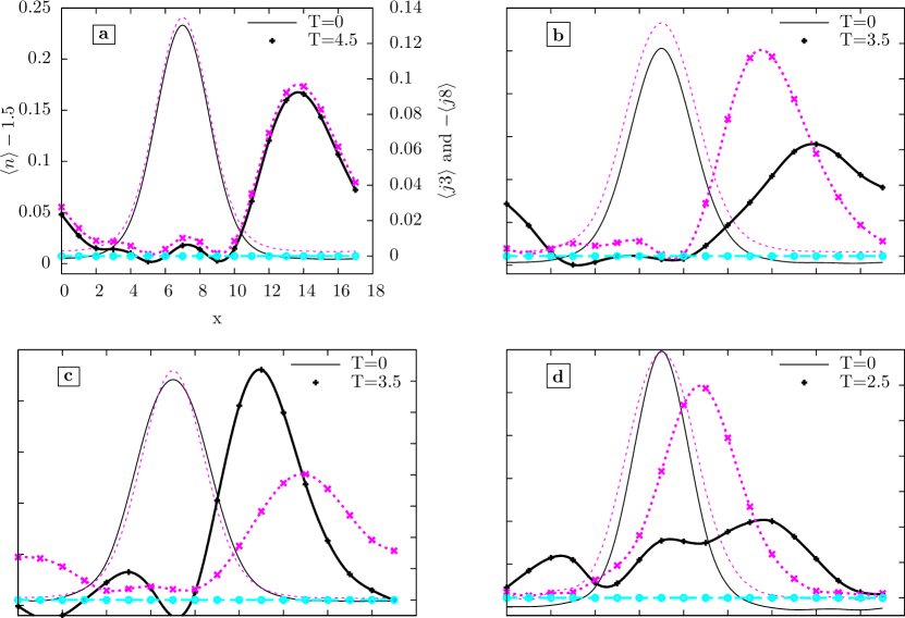
Figure 1: (color online) Snapshots of the time evolution of an additional fermion for filling $\nu=0.5$ and $U=0$ (a), $U=+1$ (b), $U=-1$ (c) and $U=+5$ (d). The initial state is a Gaussian wave packet with average momentum $k=0.6\pi$. In (b,c,d) the color density of quantum number $j^{8}$ (magenta) separates from the charge density (black), while $j^{3}$ (cyan) is constant by construction. Lines serve as guides to the eye.

To extract color and charge velocities, we applied two different extraction methods. First, the velocity can be obtained dividing the number of sites traveled by the maximum of the density by the time. It is more accurate to fit a Gaussian on the density for every time step. There is a short transient time at the beginning, followed by a plateau of constant velocity until the packet hits the boundary. We extracted the velocity of the packet when it passes the median between the initial position and the boundary and took a Gaussian averaged value around this position. As a second measure, for a definite plateau of constant velocity, we used a $L=48$ sites system with HWBCs and replaced the incident electron by an initial, small potential perturbation. The time development of this method differs mainly by the implicit stimulation of excited states around both Fermi points leading to symmetric peaks running in both directions and increasing the transient time at the start.

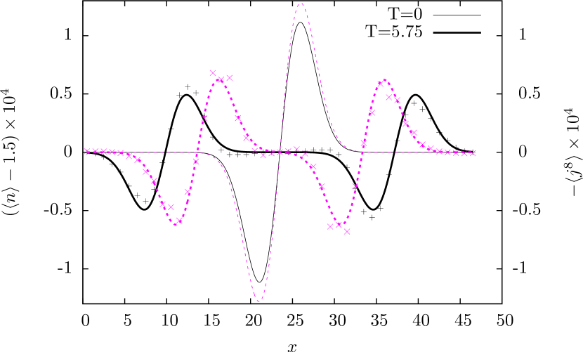
Figure 2: (color online) Snapshots of a perturbation at time $T=0$ (thin lines) and a finite time step (thick lines and data points). The dashed (solid) lines are fits to the color density of $j^{8}$ (charge density $n$) with the corresponding data points.

Fig. 2 shows snapshots of the initial and a finite time step for $U=1.5$, where the perturbation was taken to be the derivative of a Gaussian and this function was fitted on the two propagating wave packets. We find that both methods provide similar results, while the latter proved to be a considerable improvement in precision and is put forward by us as a general preferable method to extract velocities from td-DMRG.

Finally, the extracted velocities are shown as a function of the uniform interaction in Fig. 3. On top of the data, we show the expected relation for $v_{\text{col}}(U),v_{\text{ch}}(U)$ from bosonization, scaled to match the free fermion velocity. This a priori renormalization covers all direct effects that lead to deviations of the Fermi velocity due to finite width or the central momentum $k_{0}$ of the excitation and the finite size dispersion. Even for $|U|$ up to $1$, the agreement between the bosonization estimate and the numerical data is found to be excellent (dashed lines in Fig. 3). Beyond, the limits of the low energy expansion are apparently reached. However, upon extending the velocity expansion to higher order in $U$, e.g. $v_{\text{ch}}=v_{F}\sqrt{1+2U/(\pi v_{F})+aU^{2}}$, the fit already covers the complete computed range in $U$ (solid line in Fig. 3) and the parameter $a=-0.017$ has the same order and sign as the fit by Assaraf et al. Assaraf_Azaria_Caffarel_Lecheminant_PRB1999 who chose a different filling in their Monte-Carlo simulations.

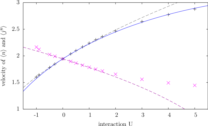
Figure 3: (color online) Velocity $v(U)$ of an initial Gaussian perturbation. Results of our td-DMRG simulations for both charge density ($+$) and color density ($\times$). The dashed lines represent bosonization results, scaled to match the DMRG velocity at $U=0$. The solid line is a fit on a next-to linear dependency in $U$.

A possible candidate for realizing the trionic phase ($U<0$) is ⁶Li for which the magnetic field dependence of the three scattering lengths has been measured Bartenstein_Altmeyer_Riedl_Geursen_Jochim_Chin_Denschlag_Grimm_Simoni_Tiesinga_Williams_Julienne_PRL2005 . The attractive $U$ interaction for magnetic fields around 1000 G can be estimated as $U_{rg}=U_{0}$, $U_{rb}=1.23U_{0}$, and $U_{gb}=1.06U_{0}$, due to the ratios in the s-wave scattering rate in each channel Bartenstein_Altmeyer_Riedl_Geursen_Jochim_Chin_Denschlag_Grimm_Simoni_Tiesinga_Williams_Julienne_PRL2005 . It is important to consider whether these anisotropies infringe on the validity of the effects observed above. In bosonization theory, anisotropy introduces new terms that couple the charge and color degrees of freedom so we would expect that high anisotropies totally destroy charge-color separation PhysRevA.80.041604 . However, small and experimentally accessible anisotropies turn out to be not decisively important. We have checked that the separation effect of color and charge densities is still visible in the simulations without much change. Even for the special cases of commensurate fillings where a stronger sensitivity on the color anisotropy may have been suspected, the qualitative behavior persists.

In summary, we have performed td-DMRG simulations of cold fermionic atoms with three hyperfine states trapped in an optical lattice. Our simulations allowed us to observe the color-charge separation in SU(3) fermionic systems in a generic non-commensurate case. We have obtained the charge and color velocities as a function of the interaction from the real-time simulations both for the attractive and repulsive case. Once we take into account finite size effects by renormalizing the non-interacting velocities, our results at weak coupling are in good agreement with bosonization calculations.

The authors acknowledge discussions with Philippe Lecheminant and Stephan Rachel. RAM is supported in part by Spanish Government grant No. FIS2009-07277, RT by a Feodor Lynen Fellowship of the Humboldt Foundation. We acknowledge the support by the Center for Functional Nanostructures (CFN), project B2.10.

References

- (1) B. A. Bernevig, D. Giuliano, and R. B. Laughlin, Phys. Rev. B 65, 195112 (2002).
- (2) R. Thomale, D. Schuricht, and M. Greiter, Phys. Rev. B 74, 024423 (2006).
- (3) R. Thomale, D. Schuricht, and M. Greiter, Phys. Rev. B 75, 024405 (2007).
- (4) Y. Kuramoto and H. Yokoyama, Phys. Rev. Lett. 67, 1338 (1991).
- (5) T. Giamarchi, Quantum Physics in One Dimension, International Series of monographs on physics, Oxford University Press (2004).
- (6) M. Bockrath et al., Nature (London) 397, 598 (1999).
- (7) P. Segovia, D. Purdie, M. Hengsberger, and Y. Baer, Nature 402, 504 (1999).
- (8) R. Losio et al., Phys. Rev. Lett. 86, 4632 (2001).
- (9) T. Lorenz et al., Nature 418, 614 (2002).
- (10) O. M. Auslaender et al., Science 308, 88 (2005).
- (11) M. Lewenstein et al., Adv. Phys. 56, 243 (2007).
- (12) M. Greiner et al., Nature 415, 39 (2002).
- (13) T. Stöferle et al., Phys. Rev. Lett. 96, 030401 (2006).
- (14) J. K. Chin et al., Nature 443, 961 .
- (15) R. Jördens et al., Nature 455, 204 (2008).
- (16) C. Kollath, U. Schollwöck, and W. Zwerger, Phys. Rev. Lett. 95, 176401 (2005).
- (17) C. Kollath and U. Schollwöck, New J. Phys. 8, 220 (2006).
- (18) T. Ulbricht and P. Schmitteckert, EPL 86, 57006 (2009).
- (19) P. Schmitteckert and G. Schneider, in High Performance Computing in Science and Engineering ’06, ed. by W. E. Nagel, W. Jäger, M. Resch, Springer, Berlin, 113 (2006).
- (20) P. Schmitteckert, in High Performance Computing in Science and Engineering ’07, ed. by W. E. Nagel, D. B. Kröner, M. Resch, Springer, Berlin, 99 (2007).
- (21) T. Ulbricht and P. Schmitteckert, EPL, (accepted for publication)(2010) .
- (22) A. Kleine et al., Phys. Rev. A 77, 013607 (2008).
- (23) C. Wu, Phys. Rev. Lett. 95, 266404 (2005).
- (24) P. Lecheminant, E. Boulat, and P. Azaria, Phys. Rev. Lett. 95, 240402 (2005).
- (25) H. Kamei and K. Miyake, J. Phys. Soc. Jpn. 74, 1911 (2005).
- (26) A. Rapp, G. Zaránd, C. Honerkamp, and W. Hofstetter, Physical Review Letters 98, 160405 (2007).
- (27) C. Honerkamp and W. Hofstetter, Phys. Rev. Lett. 92, 170403 (2004).
- (28) A. V. Gorshkov et al., arXiv:0905.2610, (unpublished).
- (29) S. Rachel et al., Phys. Rev. B 80, 180420(R) (2009).
- (30) M. Bartenstein et al., Phys. Rev. Lett. 94, 103201 (2005).
- (31) T. B. Ottenstein et al., Phys. Rev. Lett. 101, 203202 (2008).
- (32) J. H. Huckans et al., Phys. Rev. Lett. 102, 165302 (2009).
- (33) C. A. Regal, Ph.D. thesis, .
- (34) S. R. White, Phys. Rev. Lett. 69, 2863 (1992).
- (35) P. Schmitteckert, Phys. Rev. B 70, 121302(R) (2004).
- (36) A. J. Daley, C. Kollath, U. Schollwöck, and G. Vidal, J. Stat. Mech. 2004, P04005 (2004).
- (37) S. R. White and A. E. Feiguin, Phys. Rev. Lett. 93, 076401 (2004).
- (38) U. Schollwöck, Rev. Mod. Phys. 77, 259 (2005).
- (39) D. Jaksch et al., Phys. Rev. Lett. 81, 3108 (1998).
- (40) R. Assaraf, P. Azaria, M. Caffarel, and P. Lecheminant, Phys. Rev. B 60, 2299 (1999).
- (41) P. Azaria, S. Capponi, and P. Lecheminant, Phys. Rev. A 80, 041604(R) (2009).
- (42) K. Buchta, O. Legeza, E. Szirmai, and J. Sólyom, Phys. Rev. B 75, 155108(R) (2007).