Robust Independent Component Analysis by Iterative Maximization of the Kurtosis Contrast with Algebraic Optimal Step Size

Abstract

Independent component analysis (ICA) aims at decomposing an observed random vector into statistically independent variables. Deflation-based implementations, such as the popular one-unit FastICA algorithm and its variants, extract the independent components one after another. A novel method for deflationary ICA, referred to as RobustICA, is put forward in this paper. This simple technique consists of performing exact line search optimization of the kurtosis contrast function. The step size leading to the global maximum of the contrast along the search direction is found among the roots of a fourth-degree polynomial. This polynomial rooting can be performed algebraically, and thus at low cost, at each iteration. Among other practical benefits, RobustICA can avoid prewhitening and deals with real- and complex-valued mixtures of possibly non-circular sources alike. The absence of prewhitening improves asymptotic performance. The algorithm is robust to local extrema and shows a very high convergence speed in terms of the computational cost required to reach a given source extraction quality, particularly for short data records. These features are demonstrated by a comparative numerical analysis on synthetic data. RobustICA’s capabilities in processing real-world data involving non-circular complex strongly super-Gaussian sources are illustrated by the biomedical problem of atrial activity (AA) extraction in atrial fibrillation (AF) electrocardiograms (ECGs), where it outperforms an alternative ICA-based technique.

I Introduction

I-A Blind Source Separation and Independent Component Analysis

Introduced over two decades ago [1], the problem of blind source separation (BSS) consists of recovering a set of unobservable source signals from observed mixtures of the sources. Independent component analysis (ICA) aims at decomposing an observed random vector into statistically independent variables [2]. Among its numerous applications, ICA is the most natural tool for BSS in instantaneous linear mixtures when the source signals are assumed to be independent. As opposed to classical decomposition techniques such as principal component analysis (PCA), ICA can deal with a general mixing structure, even if not made up of orthogonal columns. The plausibility of the statistical independence assumption in a wide variety of fields, including telecommunications, finance and biomedical engineering, helps explain the arousing interest in this research area witnessed over the last two decades.

Mathematically, the observed random vector $\mathbf{x}\in\mathbb{C}^{L}$ is assumed to be generated according to the instantaneous linear mixing model:

$$\mathbf{x}=\mathbf{H}\mathbf{s}+\mathbf{n}$$ (1)

where the source vector $\mathbf{s}=[s_{1},s_{2},\dots,s_{K}]{{}^{\mathrm{T}}}\in\mathbb{C}^{K}$ is made of $K\leq L$ unknown mutually independent components. The elements of mixing matrix $\mathbf{H}\in\mathbb{C}^{L\times K}$ are also unknown, and so are the noise vector $\mathbf{n}$ and its probability distribution; the noise is only assumed to be independent of the sources. Our focus is on batch or block implementations, which, contrary to common belief, are not necessarily more costly than adaptive (recursive, on-line, sample-by-sample, or neural) algorithms, and are able to use more effectively the information contained in the observed signal block [3]. Given a sensor-output signal block composed of $T$ samples, ICA aims at estimating the corresponding $T$-sample realization of the source vector.

I-B Kurtosis as a Contrast Function

Since Comon’s seminal work [2], many contrast functions for ICA have been proposed in the literature, mainly based on information theoretical principles such as maximum likelihood, mutual information, marginal entropy and negentropy, as well as related non-Gaussianity measures [4, 5, 6]. Among them, the kurtosis (normalized fourth-order marginal cumulant) is arguably the most common statistics used in ICA, even if skewness has also been proposed [7]. The use of kurtosis dates back to the work of Wiggins [8], Donoho [9] and Shalvi-Weinstein [10] on blind deconvolution of seismic signals and blind equalization of single-input single-output (SISO) digital communication channels, two problems that can be related to BSS/ICA. One of the main benefits of kurtosis lies in the absence of spurious local extrema for infinite sample size when the noiseless observation model is fulfilled. This attractive feature leads to globally convergent source extraction algorithms, from which full source separation can be performed by using some form of deflation procedure [11, 12, 13, 14], even in the convolutive MIMO case [15]. Although the adequacy of kurtosis as a contrast may be objected on the basis of statistical efficiency and robustness against outliers [16], its widespread use is justified by mathematical tractability, computational convenience and robustness to finite sample effects. Theoretical evidence for its finite-sample robustness have been gathered by previous works. In [17], the sample kurtosis yields an estimate with less variance than the fourth-order moment and the fourth-order cumulant for all distributions tested, including sub-Gaussian and super-Gaussian densities. As an extension of these results, using the full expression of the fourth-order cumulant instead of the simplified form employed, e.g., in the FastICA algorithm [12, 18] is shown to improve extraction performance [19]. The computational convenience and finite sample robustness of kurtosis can be further improved by the optimal step-size iterative search proposed in the present paper. In the presence of outliers, the performance of the conventional kurtosis estimate based on sample moments can be enhanced by means of more robust alternative estimates available in the literature (see, e.g., [20, Ch. 5]).

I-C The FastICA Algorithm

The FastICA algorithm [12, 16, 18, 21] is perhaps the most popular method for ICA, due to its simplicity, convergence speed and satisfactory results in numerous applications. Indeed, the one-unit algorithm with cubic non-linearity, related to the optimization of the kurtosis contrast under prewhitening, offers cubic global convergence if the ICA model is fulfilled and the sample size tends to infinity [12, 22]. In addition, the algorithm is asymptotically efficient if the non-linearity is matched to the source probability density function [23]. The cubic non-linearity associated with kurtosis is particularly well adapted to sub-Gaussian distributions [16, 23]. Some of these desirable properties are also shared by the symmetric version of the algorithm [24]. Originally put forward in deflation mode, FastICA appeared after other kurtosis-based ICA methods such as CoM2 [2], JADE [25], CoM1 [26], or the deflation methods by Tugnait [15] or Delfosse-Loubaton [11]. A first comparison with earlier methods can be found in [27]. In the comparative study of [28], FastICA is shown to fail for weak or highly spatially correlated sources. Its convergence slows down or even fails in the presence of saddle points, particularly for short block sizes [23]. To surmount this difficulty, a simple saddle-point check method is proposed in that reference. Such a method is based on estimated component pairs and, as a result, is not applicable if only one independent component is required. Further improvements of the symmetric implementation of the algorithm are developed in [29]. All these results rely heavily on the assumption that the observed signals have been perfectly whitened or sphered before further higher-order processing. As pointed out in [30], the use of prewhitening imposes a bound on separation performance and introduces an estimation bias due to residual source correlations for short data sizes.

I-D The Complex-Valued Scenario

The FastICA algorithm was originally developed for real-valued signals only. A first extension to complex-valued sources is proposed in [31], and later shown to keep the cubic global convergence property of its real counterpart [32]. Such an extension, however, is only valid for second-order circular sources, a limitation that has motivated more recent efforts to extend the usefulness of the algorithm to non-circular sources [33, 34, 35, 36]. Reference [36] derives gradient, fixed-point and Newton-like algorithms based on the general definition of the fourth-order marginal cumulant valid for non-circular sources. In [34] the whitened observation pseudo-covariance matrix is incorporated into FastICA’s update rule to guarantee local stability at the separating solutions even in the presence of non-circular sources. For the kurtosis-based non-linearity, the resulting algorithm bears close resemblance to that derived in [33] through an ingenious approach sparing differentiation. Similar algorithms are proposed in [35] through a negentropy-based family of cost functions preserving phase information and thus adapted to non-circular sources. Such functions must be chosen in accordance with the source distributions to assure stability. Again, all the above methods rely on prewhitening. Interestingly, early methods for BSS in the complex case did not require prewhitening and were also applicable to non-circular sources [37, 38].

I-E Summary and Contributions of the Paper

This contribution presents a novel method for deflationary ICA named RobustICA [39, 40, 41]. The method is based on a general contrast function, the kurtosis, which is optimized by a computationally efficient technique based on an optimal step size (adaption coefficient). Any independent component with non-zero kurtosis can be extracted in this manner. No simplifying assumptions concerning specific type of sources (real or complex, circular or non-circular, sub-Gaussian or super-Gaussian) are involved in the derivation of the algorithm. The methodology behind RobustICA is exact line search, well known in the field of numerical optimization (see, e.g., [42]). However, classical line search techniques can only perform iterative local optimization along the search direction. By contrast, the optimal step-size technique used in RobustICA computes algebraically (i.e., without iterations) the step size globally optimizing the kurtosis in the search direction at each extracting vector update. When compared to other kurtosis-based algorithms such as the original FastICA and its variants, the method presents a number of advantages with significant practical impact:

• As opposed to [18, 31, 32] and related works, the generality of the kurtosis contrast guarantees that real- and complex-valued signals can be treated by exactly the same algorithm without any modification. Both type of source signals can be present simultaneously in a given mixture, and complex sources need not be circular. The mixing matrix coefficients may be real or complex, regardless of the source type.

• Contrary to most ICA methods, prewhitening is not required, so that the performance limitations it imposes [30] can be avoided. Sequential extraction (deflation) can be carried out, e.g., via linear regression. This feature may prove especially beneficial in ill-conditioned scenarios, the convolutive case and underdetermined mixtures.

• The algorithm can target sub-Gaussian or super-Gaussian sources in the order specified by the user. This feature enables the extraction of sources of interest when their Gaussianity character is known in advance, thus sparing a full separation of the observed mixture as well as the consequent increased complexity and estimation error.

• The optimal step-size technique provides some robustness to the presence of saddle points and spurious local extrema in the contrast function.

• The method shows a very high convergence speed measured in terms of source extraction quality versus number of operations. In the real-valued two-signal case, the algorithm converges in a single iteration, even without prewhitening.

RobustICA’s cost-efficiency and robustness are particularly remarkable for short sample length in the absence of prewhitening. In addition to presenting the method and assessing its comparative performance on synthetic data, the practical usefulness of RobustICA is illustrated in a real-world problem: the extraction of the atrial activity signal from surface electrocardiogram (ECG) recordings of atrial fibrillation. This biomedical application demonstrates that the kurtosis contrast can also be used with success in the extraction of strongly super-Gaussian sources, which, in addition, present non-circular complex distributions in this particular context.

I-F Related Work on Optimal Step-Size Iterative Methods

The convergence properties of iterative techniques are to a large extent determined by the step size, learning rate or adaption coefficient employed in their update equations. It is well known that the step-size choice sets a difficult balance between convergence speed and final accuracy (misadjustment). This trade-off has spurred the development of iterative techniques based on some form of step-size optimization. To our knowledge, research into adaptive step-size optimization can be traced back to the work of Kuzminskiy on the least mean squares (LMS) algorithm in nonstationary environments, where recursive expressions for the step size are derived [43, 44]. More recent works on the LMS algorithm such as [45, 46] seem closer to our approach, except that they aim at channel identification and the optimal step-size is computed using a quadratic cost function different from that minimized via the stochastic LMS. Our rationale is essentially different, as we aim at direct source estimation and globally optimize a non-quadratic contrast by iterating on the same signal block under the assumption of stationarity over the observation window (block or batch processing).

Amari [3, 47] puts forward adaptive rules for learning the step size in neural algorithms for BSS/ICA, more pertinent in the context of the present work. The idea is to make the step size depend on the gradient norm, in order to obtain a fast evolution at the beginning of the iterations and then a decreasing misadjustment as a stationary point is reached. These step-size learning rules, in turn, include other learning coefficients which must be set appropriately. Although the resulting algorithms are said to be robust to the choice of these coefficients, their optimal selection remains application dependent. Other guidelines for choosing the step size in natural gradient algorithms are given in [48], but are merely based on local stability conditions. In a non-linear mixing setup, Khor and co-workers put forward a fuzzy logic approach to control the learning rate of a separation algorithm based on the natural gradient [49].

In the context of batch algorithms, Regalia [50] finds bounds for the step size guaranteeing monotonic convergence of the normalized fourth-order moment of the extractor output. Such a functional is only a contrast for real-valued sources under prewhitening, a similar limitation shared by the more general class of functions considered in [51]. Determining these step-size bounds is a computational intensive task, as it involves the eigenspectrum of a Hessian matrix on a convex subset containing the unit sphere in the $K$-dimensional space. While still ensuring monotonic convergence, the optimal step-size approach that we develop herein is valid for real- and complex-valued sources, does not require prewhitening and is computationally very simple. This type of technique has already been successfully applied by the authors to other higher order contrasts such as the constant modulus or the constant power criteria in the problems of blind and semi-blind equalization of digital communication channels [52, 53, 54, 55].

I-G Organization of the Paper

The paper begins by critically reviewing the deflationary kurtosis-based FastICA algorithm and its variants in Sec. II. Then, Sec. III presents the RobustICA technique. Its experimental comparative assessment is carried out in Sec. IV. In particular, we aim at evaluating objectively the algorithms’ speed and efficiency by taking into account the cost per iteration in number of operations. A biomedical application, the extraction of atrial activity from ECG recordings of atrial fibrillation, illustrates the method’s ability to deal with non-circular complex-valued super-Gaussian sources, as reported in Sec. V. The concluding remarks of Sec. VI bring the paper to an end.

II FastICA Revisited

II-A Kurtosis-Based Optimality Criteria

In the deflation approach to ICA, an extracting vector $\mathbf{w}$ is sought so that the estimate

$$y\stackrel{{\scriptstyle\rm def}}{{=}}\mathbf{w}^{\mathrm{H}}\mathbf{x}$$ (2)

where $(\cdot)^{\mathrm{H}}$ denotes the conjugate-transpose operator, maximizes some optimality criterion or contrast function, and is hence expected to be a component independent from the others. A widely used contrast is the kurtosis, which is defined as the normalized fourth-order marginal cumulant:

$$\mathcal{K}(\mathbf{w})=\frac{\mathrm{E}\{|y|^{4}\}-2\mathrm{E}^{2}\{|y|^{2}\}-|\mathrm{E}\{y^{2}\}|^{2}}{\mathrm{E}^{2}\{|y|^{2}\}}$$ (3)

where $\mathrm{E}\{\cdot\}$ denotes the mathematical expectation. This criterion is easily seen to be insensitive to scale, i.e., $\mathcal{K}(\lambda\mathbf{w})=\mathcal{K}(\mathbf{w})$, $\forall\lambda\neq 0$. Since this scale indeterminacy is typically unimportant, we can impose, without loss of generality, the normalization $\|\mathbf{w}\|=1$ for numerical convenience. The kurtosis maximization (KM) criterion based on contrast (3) is quite general in that it does not require the observations to be prewhitened and can be applied to real- or complex-valued sources without any modification.

The KM criterion started to receive attention with the pioneering work of Wiggins [8], Donoho [9] and Shalvi-Weinstein [10] on blind deconvolution, and was later employed for source separation [11], even in the convolutive mixture scenario [15]. In the real-valued case, it was proved in [11] that the maximization of criterion $|\mathcal{K}(\mathbf{w})|$ is a valid contrast for the extraction of any source with non-zero kurtosis from model (1) after prewhitening. To avoid extracting the same source twice, the remaining unitary mixing matrix is suitably parameterized as a function of angular parameters, and function (3) iteratively maximized with respect to these angles. In the convolutive mixture scenario of [15], the contrast is maximized without parameterization. Regression is used as an alternative method to avoid extracting the same source more than once.

To simplify the source extraction, the kurtosis-based FastICA algorithm [12], [18], [21] first applies a prewhitening operation, as in [11], resulting in transformed observations with an identity covariance matrix, $\mathbf{R}_{x}\stackrel{{\scriptstyle\rm def}}{{=}}\mathrm{E}\{\mathbf{x}\mathbf{x}^{\mathrm{H}}\}=\mathbf{I}$. In the real-valued case, contrast (3) then becomes equivalent to the fourth-order moment criterion:

$$\mathcal{M}(\mathbf{w})=\mathrm{E}\{|y|^{4}\}$$ (4)

which must be optimized under a constraint, e.g., $\|\mathbf{w}\|=1$, to avoid arbitrarily large values of $y$. Under the same constraint, criteria (3) and (4) are also equivalent if the sources are complex-valued but second-order circular, i.e., the non-circular second-moment (or pseudo-covariance) matrix $\mathbf{C}_{s}\stackrel{{\scriptstyle\rm def}}{{=}}\mathrm{E}\{\mathbf{s}\mathbf{s}{{}^{\mathrm{T}}}\}$ is null, where $(\cdot){{}^{\mathrm{T}}}$ is the transpose operator without conjugation. Consequently, contrast (4) is less general than criterion (3) in that it requires the observations to be prewhitened and the sources to be real-valued, or complex-valued but circular.

II-B Contrast Optimization

Under the constraint $\|\mathbf{w}\|=1$, the stationary points of $\mathcal{M}(\mathbf{w})$ are obtained as a collinearity condition on $\mathrm{E}\{yy^{*2}\mathbf{x}\}$, where $(\cdot)^{*}$ denotes complex conjugation:

$$\mathrm{E}\bigl{\{}|\mathbf{w}^{\mathrm{H}}\mathbf{x}|^{2}\mathbf{x}\mathbf{x}^{\mathrm{H}}\bigr{\}}\mathbf{w}=\lambda\mathbf{w}$$ (5)

in which $\lambda$ is a Lagrangian multiplier. As opposed to the claims of [12], eqn. (5) is a fixed-point equation only if $\lambda$ is known, which is not the case here; $\lambda$ must be determined so as to satisfy the constraint, and thus it depends on $\mathbf{w}_{\mathrm{opt}}$, the optimal value of $\mathbf{w}$: $\lambda=\mathcal{M}(|\mathbf{w}_{\mathrm{opt}}^{\mathrm{H}}\mathbf{x}|^{4}\}$.

For the sake of simplicity, $\lambda$ is arbitrarily set to a deterministic fixed value [12], [21], so that FastICA becomes an approximate standard Newton algorithm, as eventually pointed out in [18]. In the real-valued case, the Hessian matrix of $\mathcal{M}(\mathbf{w})$ is approximated as

$$\mathrm{E}\{(\mathbf{w}{{}^{\mathrm{T}}}\mathbf{x}\mathbf{x}{{}^{\mathrm{T}}}\mathbf{w})\mathbf{x}\mathbf{x}{{}^{\mathrm{T}}}\}\approx\mathrm{E}\{\mathbf{w}{{}^{\mathrm{T}}}\mathbf{x}\mathbf{x}{{}^{\mathrm{T}}}\mathbf{w}\}\mathrm{E}\{\mathbf{x}\mathbf{x}{{}^{\mathrm{T}}}\}=\mathbf{w}{{}^{\mathrm{T}}}\mathbf{w}=\mathbf{I}$$ (6)

As a result, the kurtosis-based FastICA iteration reduces to

$$\mathbf{w}^{+}=\mathbf{w}-\frac{1}{3}\,\mathrm{E}\{\mathbf{x}(\mathbf{w}{{}^{\mathrm{T}}}\mathbf{x})^{3}\}.$$ (7)

Since $\nabla\mathcal{M}(\mathbf{w})=4\mathrm{E}\{\mathbf{x}(\mathbf{w}{{}^{\mathrm{T}}}\mathbf{x})^{3}\}$, eqn. (7) is essentially a gradient-descent update rule of the form

$$\mathbf{w}^{+}=\mathbf{w}-\mu\nabla\mathcal{M}(\mathbf{w})$$

with a fixed value for the step size, $\mu=1/12$. It follows that the kurtosis-based FastICA is a particular instance, using prewhitening and assuming sub-Gaussian sources, of the family of gradient-based algorithms proposed in [15]. Though fixed to a constant value, FastICA’s step-size choice is judicious in that it leads to cubic convergence of the algorithm for infinite sample size [18]. For short sample sizes, however, convergence may slow down and even get trapped in saddle areas and local extrema, as has been noticed in [23] and will be further illustrated in Sec. IV.

To prevent locking onto a previously extracted source, the so-called deflationary orthogonalization can be performed after each FastICA update iteration. The extracting vector is constrained to lie within the orthogonal subspace of the extracting vectors, stored in matrix $\mathbf{W}_{k}=[\mathbf{w}_{1},\mathbf{w}_{2},\dots,\mathbf{w}_{k-1}]$, found for the previous $(k-1)$ sources:

$$\mathbf{w}^{+}\leftarrow\mathbf{w}^{+}-\mathbf{W}_{k}\mathbf{W}_{k}^{\mathrm{H}}\mathbf{w}^{+}.$$ (8)

This procedure is tantamount to the Gram-Schmidt orthogonalization of $\mathbf{w}^{+}$ with respect to the columns of $\mathbf{W}_{k}$. The iteration concludes with a normalization step to guarantee the constraint $\|\mathbf{w}^{+}\|=1$:

$$\mathbf{w}^{+}\leftarrow\mathbf{w}^{+}/\|\mathbf{w}^{+}\|.$$ (9)

The algorithm can be stopped when

$$\bigl{|}1-|\mathbf{w}^{\mathrm{H}}\mathbf{w}^{+}|\bigr{|}<\epsilon$$ (10)

for a statistically significant small constant $\epsilon$, e.g., $\epsilon=\eta/T$ with $\eta<1$. The use of the transpose-conjugate operator in eqns. (8) and (10) makes them also valid in the complex case.

II-C The Complex Case

In the extension of the kurtosis-based FastICA algorithm to complex-valued scenarios [31, 32], the update rule can be expressed as

$$\mathbf{w}^{+}=\mathbf{w}-\frac{1}{2}\,\mathrm{E}\{\mathbf{x}y^{*}|y|^{2}\}$$ (11)

with $y$ given in (2). Let us define the gradient operator as $\nabla_{\mathbf{w}}=\nabla_{\mathbf{w}_{r}}+j\nabla_{\mathbf{w}_{i}}$, where $\mathbf{w}_{r}$ and $\mathbf{w}_{i}$ represent the real and imaginary parts, respectively, of vector $\mathbf{w}$; this a scaled form of Brandwood’s conjugate gradient [56]. Then, eqn. (11) is easily shown to be a gradient-descent algorithm on contrast (4) with fixed step size $\mu=1/8$. The algorithm is only valid for second-order circular sources, satisfying $\mathbf{C}_{s}=\mathbf{0}$. Recent works aiming to avoid this limitation are all based on the prewhitening assumption. Starting from the non-normalized fourth-order cumulant contrast, the KM fixed-point (KM-F) algorithm of [36] assigns the current gradient to the extracting vector

$$\mathbf{w}^{+}=\mathrm{E}\{|y|^{2}y^{*}\mathbf{x}\}-2\mathrm{E}\{|y|^{2}\}\mathrm{E}\{y^{*}\mathbf{x}\}-\mathrm{E}\{{y^{*}}^{2}\}\mathrm{E}\{y\mathbf{x}\}$$ (12)

before the orthogonalization and normalization steps described by eqns. (8) and (9). A modification of [31] is proposed in [34] leading to the so-called non-circular FastICA (nc-FastICA) algorithm. For contrast (4), the modified update rule reads:

$$\mathbf{w}^{+}=\mathbf{w}-\frac{1}{2}\,\mathrm{E}\{|y|^{2}y^{*}\mathbf{x}\}+\frac{1}{2}\mathrm{E}\{\mathbf{x}\mathbf{x}{{}^{\mathrm{T}}}\}\mathrm{E}\{{y^{*}}^{2}\}\mathbf{w}^{*}.$$ (13)

By taking into account the whitened observation pseudo-covariance matrix in the last term, the nc-FastICA algorithm becomes locally stable at the separation solutions even in the presence of non-circular sources. The complex fixed-point algorithm (CFPA) of [33] turns out to rely on a very similar update rule, obtained through an alternative approach not based on differentiation.

III RobustICA

III-A Exact Line Search on the Kurtosis Contrast

Without simplifying assumptions, a simple quite natural alternative to FastICA consists of performing exact line search of the absolute kurtosis contrast (3):

$$\mu_{\mathrm{opt}}=\arg\underset{\mu}{\max}\>|\mathcal{K}(\mathbf{w}+\mu\mathbf{g})|.$$ (14)

The search direction $\mathbf{g}$ is typically (but not necessarily) the gradient, $\mathbf{g}=\nabla_{\mathbf{w}}\mathcal{K}(\mathbf{w})$, which is given by (cf. [13, 15]):

$$\nabla_{\mathbf{w}}\mathcal{K}(\mathbf{w})=\frac{4}{\mathrm{E}^{2}\{|y|^{2}\}}\left\{\mathrm{E}\{|y|^{2}y^{*}\mathbf{x}\}-\mathrm{E}\{y\mathbf{x}\}\mathrm{E}\{{y^{*}}^{2}\}-\frac{\bigl{(}\mathrm{E}\{|y|^{4}\}-|\mathrm{E}\{y^{2}\}|^{2}\bigr{)}\mathrm{E}\{y^{*}\mathbf{x}\}}{\mathrm{E}\{|y|^{2}\}}\right\}.$$

Exact line search is in general computationally intensive and presents other limitations [42], which explains why, despite being a well-known optimization method, it is very rarely used in practice. Indeed, the one-dimensional optimization in eqn. (14) must typically be performed by means of numerical algorithms that are not guaranteed to find the global optimum along the search direction. However, for criteria that can be expressed as polynomials or rational functions of $\mu$, such as the kurtosis, the constant modulus [57], [55] and the constant power [58], [54] contrasts, the globally optimal step size $\mu_{\mathrm{opt}}$ can easily be determined algebraically by finding the roots of a low-degree polynomial. The RobustICA algorithm is derived from the application of this idea to the kurtosis contrast, as detailed next. A freely available Matlab implementation can be found in [59].

At each iteration, RobustICA performs an optimal step-size (OS) based optimization comprising the following steps:

• Compute the OS polynomial coefficients.

  For the kurtosis contrast, the OS polynomial is given by:

  $$p(\mu)=\sum_{k=0}^{4}a_{k}\mu^{k}.$$ (15)

  The coefficients $\{a_{k}\}_{k=0}^{4}$ can easily can be obtained at each iteration from the observed signal block and the current values of $\mathbf{w}$ and $\mathbf{g}$. Their expressions are found in the Appendix. Numerical conditioning in the determination of $\mu_{\mathrm{opt}}$ can be improved by normalizing the gradient vector beforehand.

• Extract OS polynomial roots $\{\mu_{k}\}_{k=1}^{4}$.

  The roots of the 4th-degree polynomial (quartic) can be found at practically no cost using standard algebraic procedures such as Ferrari’s formula, known since the 16th century [42]. Indeed, the complexity of this step is negligible compared with the calculation of the statistics required in the previous step. Details about computational cost are given in Sec. III-E.

• Select the root leading to the absolute maximum of the contrast along the search direction:

  $$\mu_{\mathrm{opt}}=\arg\underset{k}{\max}\>|\mathcal{K}(\mathbf{w}+\mu_{k}\mathbf{g})|.$$ (16)

  This can be done at a negligible cost from the coefficients computed in step S1, as detailed in the Appendix.

• Update $\mathbf{w}^{+}=\mathbf{w}+\mu_{\mathrm{opt}}\mathbf{g}$.

• Normalize as in eqn. (9).

As in [15], the extracting vector normalization in step S5 is performed to fix the ambiguity introduced by the the scale invariance of contrast (3), and does not stem from prewhitening. The same stopping criterion as in FastICA [cf. eqn. (10)] can also be employed to check the convergence of the above algorithm. The generality of contrast (3) guarantees that RobustICA is able to separate real and complex (possibly non-circular) sources without any modification. These features will be illustrated in the experiments of Secs. IV–V.

III-B Extraction of Sources with Known Kurtosis Sign

The method described above aims at maximizing the absolute kurtosis, and is thus able to extract sources with positive or negative kurtosis. In many applications, some information may be known in advance about the source(s) of interest. For example, the atrial activity time-domain signal in atrial fibrillation electrocardiograms (Sec. V), and especially in atrial flutter episodes, typically lies in the sub-Gaussian source subspace. The ventricular activity sources are usually impulsive and thus super-Gaussian. If only a few of these sources are desired, separating the whole mixture would incur an unnecessary computational cost and, in the case of sequential extraction, an increased source estimation inaccuracy due to error accumulation through successive deflation stages. A wiser alternative consists of extracting the desired type of sources exclusively.

RobustICA can easily be modified to deal with these situations by targeting a source with specific kurtosis sign $\varepsilon$. After computing the roots of the step-size polynomial, one simply needs to replace (16) by

$$\mu_{\mathrm{opt}}=\mathrm{arg}\>\underset{k}{\mathrm{max}}\;\varepsilon\mathcal{K}(\mathbf{w}+\mu_{k}\mathbf{g})$$ (17)

as best root selection criterion. If no source exists with the required kurtosis sign, the algorithm may converge to a non-extracting local extrema, but will tend to produce components with maximal or minimal kurtosis from the remaining signal subspace when $\varepsilon=1$ or $\varepsilon=-1$, respectively. The algorithm can also be run by combining global line maximizations (17) and (16) for sources with known and unknown kurtosis sign, respectively, in any desired order.

III-C Deflation

To extract more than one independent component, the Gram-Schmidt-type deflationary orthogonalization procedure proposed for FastICA [12], [18], [21] (see Sec. II-B) can also be used in conjunction with RobustICA under prewhitening, even if prewhitening is not mandatory for this method. After step S4, the updated extracting vector is constrained to lie in the orthogonal subspace of the extracting vectors previously found [eqn. (8)]. In the linear regression approach to deflation [15], after convergence of the search algorithm the contribution of the estimated source $\hat{s}$ to the observations is computed via the minimum mean square error solution to the linear regression problem $\mathbf{x}=\mathbf{\hat{h}}\hat{s}$. The observations are then deflated as $\mathbf{x}\leftarrow(\mathbf{x}-\mathbf{\hat{h}}\hat{s})$ before re-initializing the algorithm in the search for the next source. If prewhitening is not performed and the mixture is not unitary, orthogonalization is no longer an option and an alternative procedure like regression becomes compulsory.

III-D A Quick Look at Convergence

The theoretical study of RobustICA’s convergence characteristics in the general case is beyond the scope of the present paper. In the real-valued two-signal scenario, however, the algorithm converges to the global optimum in a single iteration, even without prewhitening. The proof relies on the scale invariance property of contrast (3) and follows straightforward geometrical arguments. Suppose that the initial (non-zero) extracting vector $\mathbf{w}_{0}$ has an orientation of $\alpha_{1}$ rad with respect to one of the axis vectors spanning $\mathbb{R}^{2}$. In polar coordinates, the gradient at $\mathbf{w}_{0}$ can be expressed as

$$\mathbf{g}_{0}=\nabla\mathcal{K}(\mathbf{w}_{0})=\frac{\partial\mathcal{K}(\mathbf{w}_{0})}{r\partial\theta}\mathbf{u}_{\theta}+\frac{\partial\mathcal{K}(\mathbf{w}_{0})}{\partial r}\mathbf{u}_{r}$$

where $\mathbf{u}_{\theta}$ and $\mathbf{u}_{r}$ denote the unit vectors in the radial and ortho-radial directions, respectively. The radial component can be computed as

$$\frac{\partial\mathcal{K}(\mathbf{w}_{0})}{\partial r}=\underset{\alpha\rightarrow 0}{\lim}\>\frac{\mathcal{K}(\mathbf{w}_{0}+\alpha\mathbf{u}_{r})-\mathcal{K}(\mathbf{w}_{0})}{\alpha}=0$$

since $\mathbf{w}_{0}\propto\mathbf{u}_{r}$ and the numerator is null for any $\alpha$ by virtue of the contrast scale invariance. Vector $\mathbf{g}_{0}$ is orthogonal to $\mathbf{w}_{0}$ and its orientation is thus $\alpha_{2}=\alpha_{1}\pm\pi/2$ rad. Now, as $\mu$ varies in $\mathbb{R}$, the orientation of vector $\mathbf{w}_{0}+\mu\mathbf{g}_{0}$ spans a $\pi$-rad interval, which corresponds to the full solution space up to admissible sign and scale ambiguities in the two-signal case. Hence, the optimal step-size technique described in Sec. III-A will find the global optimum of the absolute kurtosis contrast in a single step. Although this result is not easily generalized to more than two signals, it gives a glimpse of RobustICA’s speed of convergence measured in terms of iterations. By construction of the algorithm, the OS procedure guarantees at least monotonic convergence of the kurtosis contrast to a local extremum for any initial condition (cf. [50, 51]). Also by construction, consecutive gradient vectors are orthogonal in the sense that $\text{I$\!$Re}\{\mathbf{g}^{\mathrm{H}}\mathbf{g}^{+}\}=0$, with $\mathbf{g}^{+}=\nabla\mathcal{K}(\mathbf{w}^{+})$. This gradient orthogonality may slow down convergence in high-dimensional extracting vector spaces.

III-E Computational Complexity

In the literature, complexity is commonly measured in terms of iterations. Such a measure is unfair in that an algorithm requiring few iterations to converge may involve heavy computations at each iteration. The average time taken by an algorithm to achieve a solution, another complexity measure used in some works [29, 36], does not take into account the fact that computation time depends on the actual algorithmic implementation. For instance, when using the popular Matlab technical computing environment, the execution time can be considerable reduced if loops are replaced by vector-wise operations. These observations point out that the number of real-valued floating point operations (flops) required for an algorithm to reach a solution arises as a more objective measure of complexity. A flop is considered as a product followed by an addition and, in practical implementations, would naturally correspond to a multiply-and-accumulate cycle in a digital signal processor. In the signal extraction problem, the total cost of the extraction can be computed as the product of the number of iterations, the cost per iteration per source and the number of extracted sources. The prewhitening stage, if performed, adds around $2K^{2}T$ flops ($8K^{2}T$ in the complex case) to the total cost when computing the economy singular value decomposition (SVD) of the data matrix [60]. The complexity per source per sample is given by the total cost divided by $KT$.

Table I summarizes the main computations per iteration required by RobustICA and FastICA, for both the real-valued and complex-valued scenarios; flop count details can be found in [61]. Expectations are replaced by sample averages over the observed signal block. The sample size $T$ is assumed to be sufficiently large, so that only dominant terms (with a cost depending on $T$) are considered. For the sake of comparison, the complex extension of FastICA developed in [31, 32] (only valid for second-order circular sources) is considered in the corresponding entry of Table I. The CFPA [33] and nc-FastICA [34] algorithms [eqn. (13)] have essentially the same cost as FastICA in the complex case; it suffices to add an initial burden of $L(2L+1)T$ flops due to the computation of the pseudo-covariance matrix. The KM-F algorithm [36] [eqn. (12)] takes as many operations per iteration as RobustICA’s gradient computation save for the term $\mathrm{E}\{|y|^{4}\}$, i.e., $(14L+5)T$ flops. RobustICA’s iterations are generally more expensive than FastICA’s and its variants. However, as will be demonstrated in the next section, each RobustICA iteration is more effective in the search of good extraction solutions, so that the overall complexity is actually lower than FastICA’s for the same extraction accuracy. Furthermore, in some cases FastICA cannot reach RobustICA’s accuracy.

IV Experimental Analysis

The following experimental analysis evaluates RobustICA’s convergence characteristics, source extraction quality and computational complexity in several simulation conditions involving synthetic data. In the real case (Secs. IV-A–IV-D), we use the original FastICA algorithm with cubic non-linearity [eqn. (7)] as a benchmark, as it offers the fastest convergence speed among the previously proposed kurtosis-based source extraction methods. In the complex case (Sec. IV-E), we compare RobustICA to recent FastICA variants capable of dealing with non-circular sources. The processing of real data is reported in Sec. V.

IV-A Robustness to Saddle Points

The first experiment tests the comparative convergence characteristics of RobustICA as well as its robustness to saddle points degrading the performance of the FastICA algorithm for short sample sizes [23]. Independent realizations of two uniformly distributed sources are mixed through Givens rotations of random angle $\theta$. The FastICA and RobustICA algorithms are run on the same mixed data with a sufficiently small termination test $\eta=0.5\times 10^{-6}$. As a natural measure of extraction quality, we employ the average signal mean square error (SMSE), a contrast-independent criterion defined as

$$\text{SMSE}=\frac{1}{K}\sum_{k^{\prime}=1}^{K}\text{SMSE}_{k^{\prime},\ell^{\prime}(k^{\prime})}$$ (18)

where $\text{SMSE}_{k,\ell}=\mathrm{E}\{|s_{k}-\alpha_{\ell}\hat{s}_{\ell}|^{2}\}$, with $\alpha_{\ell}=\mathrm{E}\{s_{k}\hat{s}_{\ell}^{*}\}/\mathrm{E}\{|\hat{s}_{\ell}|^{2}\}$. Signal pairs $(s_{k^{\prime}},\hat{s}_{\ell^{\prime}(k^{\prime})})$ are chosen in increasing SMSE order as $\bigl{(}k^{\prime},\ell^{\prime}(k^{\prime})\bigr{)}=\arg\underset{k,\ell}{\min}\;\text{SMSE}_{k,\ell}$ and, once selected, are no longer taken into account in the pairing of the remaining sources. When the source estimation is good enough, this ‘greedy’ algorithm allows an optimal permutation and scaling of the estimated sources $\{\hat{s}_{k}\}_{k=1}^{K}$ before evaluating the performance index. In the current setting, the global matrix $\mathbf{G}=\mathbf{W}{{}^{\mathrm{T}}}\mathbf{H}$ is also a Givens rotation of parameter $\Delta\theta=(\theta-\hat{\theta})$, where $\hat{\theta}$ is the rotation angle implicitly estimated by the separation methods.

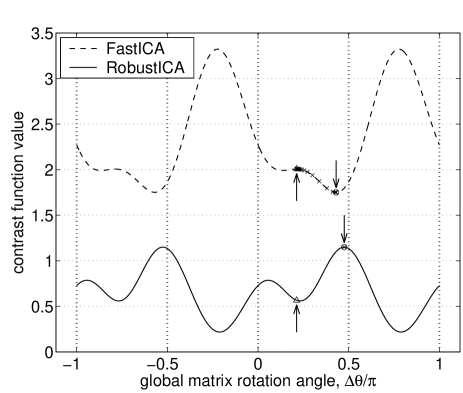
(b)

Figure 1: Contrast function values and trajectories for an orthogonal mixture realization of two uniformly distributed sources composed of $T=50$ samples. Dashed line: FastICA’s contrast function (4). Solid line: RobustICA’s contrast function (3). Triangle markers and upward arrows: initial positions. Cross markers: algorithms’ solutions after each iteration. Round markers and downward arrows: final solutions. Vertical dotted lines: satisfactory separation solutions up to sign and permutation. Subplots (a)–(b) correspond to two different extracting vector initializations over the same mixture realization.

For a particular signal realization, Fig. 1 plots the contrast functions of the respective algorithms [kurtosis (3) for RobustICA and fourth-order moment (4) for FastICA] over the optimization interval. The small sample size (here 50 samples) smears FastICA’s contrast function, whose local minima tend to form saddle regions while moving away from the valid separation solutions $\Delta\theta=k\pi/2$ rad, $k\in\mathbb{Z}$. The negative impact of short data length is less manifest for the kurtosis contrast optimized by RobustICA. For the particular initialization shown in Fig. 1(a), FastICA gets trapped inside a saddle area between two separation solutions, yielding a final SMSE of $-7.8$ dB after 29 iterations. Depending on the initialization, FastICA can also converge to the other local minimum with $\mathrm{SMSE}=-13.4$ dB, taking up to 24 iterations [cf. Fig. 1(b)]. By contrast, RobustICA consistently converges to the solutions near $\Delta\theta=\pm\pi/2$ rad with $-22.2$-dB SMSE in a single iteration for all initializations, as expected from the theoretical analysis of Sec. III-D. Figure 2 shows the scatter plot of final SMSE values for both methods over 1000 independent mixture realizations; Table II summarizes the average performance parameters for different sample size values between 50 and 150.

RobustICA provides a faster more robust performance, especially for short data sizes. The algorithm’s robustness to initialization is also demonstrated in [39]. These results support the finite sample analysis of [17], where the kurtosis is shown to present lower variance than the fourth-order moment. Similarly, the full expression of the fourth-order cumulant yields improved extraction performance compared with the fourth-order moment used in the FastICA algorithm [19]. The optimal step-size technique used in RobustICA further enhances the finite-sample benefits of the kurtosis contrast.

IV-B Performance-Complexity Trade-off

A wireless telecommunications scenario is simulated by considering noiseless orthogonal random mixtures of $K$ unit-power independent BPSK sources observed at the output of an $L=K$ element array in signal blocks of $T$ samples. The search for each extracting vector is initialized with the corresponding canonical basis vector, and is stopped at a fixed number of iterations. The SMSE performance index (18) is averaged over 1000 independent random realizations of the sources and the mixing matrix. Extraction solutions are computed directly from the observed unitary mixtures (‘FastICA’ and ‘RobustICA’ legend labels) and after a prewhitening stage based on the SVD of the observed data matrix (‘pw+FastICA’, ‘pw+RobustICA’).

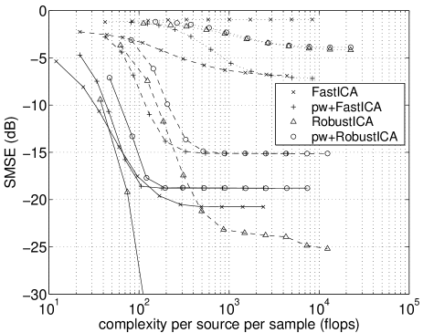
Figure 3: Average extraction quality as a function of computational cost for different mixture sizes $K$, with signal blocks composed of $T=150$ samples and 1000 mixture realizations. Solid lines: $K=5$. Dashed lines: $K=10$. Dotted lines: $K=20$.

Fig. 3 summarizes the performance-complexity variation obtained for $T=150$ samples and different values of the mixture size $K$. The best fastest performance is provided by RobustICA without prewhitening: a given performance level is achieved with lower cost or, alternatively, an improved extraction quality is reached with a given complexity. Although not shown in the plot, the method gets below the $-60$-dB SMSE level for $K=5$ sources in this experiment. The use of prewhitening worsens RobustICA’s performance-complexity trade-off and, due to the finite sample size, imposes the same SMSE bound for the two methods. Using prewhitening, FastICA improves considerably and becomes slightly faster than RobustICA with prewhitening, especially when the mixture size increases. Fig. 4 displays the quality-cost trade-off for $K=10$ sources and different block length values. Improved performance bounds can be achieved by RobustICA if avoiding prewhitening, even for short data sizes.

IV-C Efficiency

We now evaluate the methods’ performance for a varying block sample size $T$. Extractions are obtained by limiting the number of iterations per source, as explained above. To make the comparison meaningful, the overall complexity is fixed at 400 flops/source/sample for all tested methods. Accordingly, since RobustICA is more costly per iteration than FastICA, it performs fewer iterations per source. Fig. 5 displays the average SMSE curves for different number of sources $K$. For moderate $K$, RobustICA is considerably more efficient than the other methods, as shown by the steeper slope of its curve, achieving the same extraction performance with much smaller signal blocks. Prewhitening smoothens FastICA’s and RobustICA’s performance trends, which become comparable. As $K$ increases, FastICA with prewhitening becomes more efficient.

IV-D Performance in the Presence of Noise

Figure 6 assesses the comparative performance of RobustICA in the presence of noise for $K=10$ sources, different sample sizes and a fixed complexity of 400 flops/source/sample. Isotropic additive white Gaussian noise is added to the observations, with a signal-to-noise ratio (SNR) given by

$$\mathrm{SNR}=\frac{\mathrm{trace}(\mathbf{H}\mathbf{H}^{\mathrm{H}})}{\sigma_{n}^{2}L}=\frac{1}{\sigma_{n}^{2}}$$

where $\sigma_{n}^{2}$ denotes the noise power at each sensor output. The minimum mean square error (MMSE) receiver is shown as a performance bound for linear detection. RobustICA appears more robust to additive noise, as it obtains an improved SMSE performance for the same noise level or, alternatively, it tolerates more noise without sacrificing performance. At high SNR, RobustICA achieves a lower performance flooring than FastICA and, for sufficient sample size, it attains the MMSE bound, employing three times fewer iterations than the other method in this experiment. Analogous results involving noise data are reported in [40].

IV-E Complex-Valued Mixtures

To briefly test RobustICA’s performance on complex-valued synthetic mixtures of non-circular sources, we repeat the experiment of Sec. IV-B but using random unitary mixing matrices. The method is compared with the KM-F algorithm of [36] and the nc-FastICA algorithm of [34] with kurtosis-based non-linearity, similar to the CFPA algorithm of [33] (Sec. II-C). The quality-cost trade-off of the three algorithms for different block sizes is shown in Fig. 7. Once more, without the performance limitations imposed by prewhitening, RobustICA proves superior to the other methods. Performances become similar under prewhitening imposed to both methods, as FastICA improves whereas RobustICA degrades.

V Processing Real Data with RobustICA

Although good performance is obtained with sub-Gaussian sources [23] as in the above numerical experiments, the use of kurtosis as a general contrast function has been discouraged on the basis of poor asymptotic efficiency for super-Gaussian sources and lack of robustness to outliers [16], because the analysis was restricted to FastICA only. This section reports a biomedical application involving non-circular complex strongly super-Gaussian sources where the kurtosis contrast, optimized by the RobustICA technique, shows satisfactory results.

V-A Atrial Activity Extraction in Atrial Fibrillation Episodes

Atrial fibrillation (AF) is the most common cardiac arrhythmia encountered in clinical practice, affecting up to 10% of the population over 70 years of age [62]. The trouble is characterized by an abnormal atrial electrical activation, whereby the organized wavefront propagation in normal sinus rhythm is replaced by several wavelets wandering around the atria in a disorganized manner. This disorderly electrical activation causes an inefficient atrial mechanical function and leads to an increased risk of blood-clot formation and stroke. Despite its incidence, prevalence and risks of serious complications, the understanding of the generation and self-perpetuation mechanisms of this disease is still unsatisfactory.

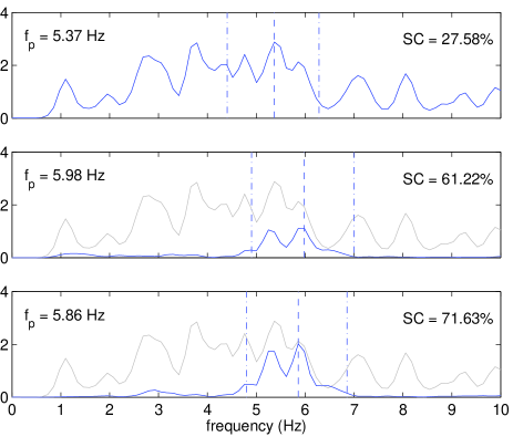
Figure 9: Atrial activity extraction in atrial fibrillation ECGs. Frequency spectra of the signals shown in Fig. 8. Top: power spectral density of signal V1 from the first patient of the database. Middle: power spectral density of AA contribution to lead V1 estimated by FastICA-SOBI from the 12-lead ECG. Bottom: power spectral density of AA contribution to lead V1 estimated by RobustICA from the 12-lead ECG. Values on the left-hand side and dashed lines: dominant frequency. Values on the right-hand side: spectral concentration. Dash-dotted lines: bounds used in the computation of spectral concentration. Only relative amplitudes are relevant on the vertical axes.

Over recent years, signal processing has helped cardiologists in shedding some light over AF, as certain features of the atrial activity (AA) signal recorded in the surface ECG provide information about the arrhythmia. The dominant frequency of the AA signal is shown to be related to the refractory period of atrial myocardium cells, and thus to the degree of evolution of the disease and the probability of spontaneous cardioversion (return to normal sinus rhythm) [63]. The analysis and characterization of AA from the ECG requires the previous suppression of interference such as the QRST complex of ventricular electrical activation (or ventricular activity, VA), artifacts and noise. Figure 8(top) shows a 5-second segment of precordial lead V1 from an AF patient’s ECG; its power spectral density, estimated through Welch’s averaged periodogram method as in [64] (averaged 8192-point FFT of 4096-point Hamming-windowed segments with 50% overlap), is shown in Fig. 9(top). The mixture of VA and AA can usually be perceived in this lead as one of its electrodes lies close to the atria.

A recent approach to AA extraction relies on the observation that AA and VA can be considered statistically independent phenomena [65]. Techniques for the separation of independent signals such as PCA and ICA can then be applied on the 12-lead ECG to search for the AA source, thus allowing the reconstruction of AA in all leads free from VA and other interference. Prior information on the atrial source, in particular its narrowband character and near-Gaussian behavior, can be exploited to improve AA extraction performance. In [64], the kurtosis-based FastICA method is first applied to extract impulsive interference, essentially the VA, from the ECG recording. The remaining sources contain mixtures of AA and noise, which, through a kurtosis-based test, are selected and passed on as inputs to the second-order blind identification (SOBI) method [66]. Through the joint approximate diagonalization of the input correlation matrices at several time lags, SOBI is particularly suited to the separation of narrowband sources. In this application, the correlation lags are chosen in accordance with typical AF cycle length values [64].

V-B Application of RobustICA to AA Extraction

AA is a narrowband signal, so that its frequency-domain representation is sparse and can thus be considered to stem from an impulsive distribution with high kurtosis value. Indeed, when mapping certain signals from the time domain to the frequency or the wavelet domains, the statistics of the sources tend to become less Gaussian, as observed in [67] in the context of another biomedical problem. Relying on this simple observation, RobustICA can be applied on the ECG recording after transformation into the frequency domain. It is expected that the $f$-domain AA source be found among the first extracted components (typically those with higher kurtosis values); its time course can then be recovered by transforming back into the time domain.

This idea is tested on a database of 35 standard ECG segments recorded from 34 different AF sufferers. Each segment represents an observation window of around 12 seconds sampled at 1 kHz. Baseline wander and high-frequency interference are suppressed by zero-phase Chebyshev type-II highpass and lowpass filters with cut-off frequencies of 0.5 and 30 Hz, respectively. The filtered 12-lead ECG data are then spatially prewhitened before being passed on to the FastICA-SOBI method of [64], which performs all operations in the time domain. Concerning the RobustICA method, the prewhitened filtered recordings are first transformed into the frequency domain by the zero-padded 16384-point FFT. The sources extracted in the $f$-domain are then transformed back to the time domain via the inverse FFT and truncated to their original length for further analysis. The AA source is automatically selected as the extracted component with dominant peak in the interval $[3,9]$ Hz, the typical AF frequency band. The percentage of signal power around the dominant peak, or spectral concentration (SC), has been shown to correlate with AA extraction quality [64], and is hence used as a measure of performance. Power spectra are estimated by Welch’s method with the same parameters as in [64]. The same initialization, maximum number of iterations per source and termination criterion are used for FastICA and RobustICA.

Figure 8(middle)–(bottom) shows a 5-second segment of the AA reconstructed by the two methods in lead V1 from the first patient of the AF ECG database. The corresponding frequency spectra, together with the estimated dominant peak position and the associated SC values, are shown in Fig. 9(middle)–(bottom). As can be seen in the intervals between successive heartbeats, RobustICA obtains a more accurate estimate of the AA taking place in lead V1, as quantified by a higher SC value, requiring a total of 698 iterations or around $2721.8\times 10^{6}$ flops to separate the whole mixture (53 iterations or $206.7\times 10^{6}$ flops if stopped at the AA source, found in the 3rd extracted component), for 1178 iterations or $391.1\times 10^{6}$ flops by FastICA (AA source in the 9th component). Performance parameters averaged over the whole dataset are summarized in Table III. A cost of about $3.5\times 10^{6}$ flops due to prewhitening should be added to the complexity figures. If stopped at the AA source, RobustICA only requires an average of $62\pm 41$ iterations or $241.3\pm 159.9\times 10^{6}$ flops. Remark that, according to Table I, RobustICA’s cost per iteration is about an order of magnitude greater than FastICA’s in this particular setting. These results confirm that RobustICA achieves an improved AA signal extraction quality with virtually identical dominant frequency estimate at a comparable complexity relative to the alternative two-stage technique. As a measure of second-order circularity, the ratio $|\mathrm{E}\{s^{2}\}|/\mathrm{E}\{|s|^{2}\}$ averaged over all $f$-domain sources extracted by RobustICA is $0.85\pm 0.02$. Since the non-circular second-order moment $\mathrm{E}\{s^{2}\}$ cannot be considered to be null, complex-valued extensions of FastICA such as those proposed in [31, 32] would not be expected to perform well in this context; more recent variants such as the KM-F and nc-FastICA algorithms [36, 34] (Sec. II-C) should be more successful. More importantly, the average kurtosis of the frequency-domain sources extracted by RobustICA in the frequency domain is $231$, whereas that of the AA sources equals $731$. These are strongly super-Gaussian signals.

VI Conclusions

Kurtosis has long been known to be a valid contrast for independent source extraction in instantaneous as well as convolutive linear mixtures, whether the sources are real or complex, circular or non-circular, sub-Gaussian or super-Gaussian, and whether prewhitening is performed. The global maximizer of this contrast across the search direction can be obtained algebraically at each extracting filter update iteration, giving rise to the RobustICA method developed in this work. Among other interesting features naturally inherited from the kurtosis contrast, RobustICA can process real- and complex-valued (possibly non-circular) sources and does not require prewhitening. As a result, the method is more tolerant than whitening-based techniques to residual source correlations likely to appear in short data records. In addition, the optimal step-size approach endows the method with an increased robustness to initialization and saddle points, particularly in small observation windows. The computational complexity required to reach a given source extraction quality has been put forward as a natural objective measure of convergence speed for BSS/ICA algorithms. Without the performance limitations imposed by second-order preprocessing (whitening), RobustICA proves computationally faster and more efficient than the popular kurtosis-based FastICA algorithm with asymptotic cubic global convergence and some of its most recent variants. RobustICA’s ability to process real-world non-circular complex strongly super-Gaussian signals has been successfully illustrated by the extraction of atrial activity in atrial fibrillation ECG recordings. In conclusion, the RobustICA method, although conceptually simple, presents a number of benefits that make it particularly attractive in practical BSS/ICA settings. Extensions to convolutive scenarios such as blind SISO and MIMO channel deconvolution are also possible with few modifications. An illustration of the optimal step-size technique on the kurtosis contrast in the SISO case is reported in [52]. The MIMO case calls essentially for the definition of appropriate deflation procedures along the lines of [15], which should be the subject of fresh investigations. More robust cumulant estimates (see, e.g., [20, Ch. 5] and references therein) would increase the method’s ability to handle outliers, and would be another interesting avenue for the continuation of this work.

Derivation of the Optimal Step-Size Polynomial

Contrast $\mathcal{K}$ evaluated at $\mathbf{w}+\mu\mathbf{g}$ becomes a function of $\mu$ only, and is given by the rational fraction

$$\mathcal{K}(\mu)=\frac{\mathrm{E}\{|y^{+}|^{4}\}-|\mathrm{E}\{(y^{+})^{2}\}|^{2}}{\mathrm{E}^{2}\{|y^{+}|^{2}\}}-2=\frac{P(\mu)}{Q^{2}(\mu)}-2$$ (19)

where $y^{+}=y+\mu g$, $y=\mathbf{w}^{\mathrm{H}}\mathbf{x}$, $g=\mathbf{g}^{\mathrm{H}}\mathbf{x}$, $P(\mu)=P_{1}(\mu)-|P_{2}(\mu)|^{2}$, $P_{1}(\mu)=\mathrm{E}\{|y^{+}|^{4}\}$, $P_{2}(\mu)=\mathrm{E}\{(y^{+})^{2}\}$ and $Q(\mu)=\mathrm{E}\{|y^{+}|^{2}\}$. Let us denote

$$a=y^{2}\qquad b=g^{2}\qquad c=yg\qquad d=\text{I$\!$Re}(yg^{*}).$$

After some tedious but otherwise straightforward algebraic manipulations, the above polynomials turn out to be:

$$P(\mu)=\sum_{k=0}^{4}h_{k}\mu^{k}\qquad\qquad Q(\mu)=\sum_{k=0}^{2}i_{k}\mu^{k}$$ (20)

where

$$h_{0} = \mathrm{E}\{|a|^{2}\}-|\mathrm{E}\{a\}|^{2},\quad h_{1}=4\mathrm{E}\{|a|d\}-4\text{I$\!$Re}(\mathrm{E}\{a\}\mathrm{E}\{c^{*}\})$$

$$h_{2} = 4\mathrm{E}\{d^{2}\}+2\mathrm{E}\{|a||b|\}-4|\mathrm{E}\{c\}|^{2}-2\text{I$\!$Re}(\mathrm{E}\{a\}\mathrm{E}\{b^{*}\})$$

$$h_{3} = 4\mathrm{E}\{|b|d\}-4\text{I$\!$Re}(\mathrm{E}\{b\}\mathrm{E}\{c^{*}\}),\quad h_{4}=\mathrm{E}\{|b|^{2}\}-|\mathrm{E}\{b\}|^{2}$$

$$i_{0} = \mathrm{E}\{|a|\},\quad i_{1}=2\mathrm{E}\{d\},\quad i_{2}=\mathrm{E}\{|b|\}.$$ (21)

Hence, the derivative of $\mathcal{K}(\mathbf{w}+\mu\mathbf{g})$ with respect to $\mu$ reads

$$\dot{\mathcal{K}}(\mu)=\frac{\dot{P}(\mu)Q(\mu)-2P(\mu)\dot{Q}(\mu)}{Q^{3}(\mu)}=\frac{p(\mu)}{Q^{3}(\mu)}.$$ (22)

Relating eqns. (20)–(22), polynomial $p(\mu)$ is given by eqn. (15) with

$$a_{0} =-2h_{0}i_{1}+h_{1}i_{0}\quad a_{1}=-4h_{0}i_{2}-h_{1}i_{1}+2h_{2}i_{0}$$

$$a_{2} =-3h_{1}i_{2}+3h_{3}i_{0}\quad a_{3}=-2h_{2}i_{2}+h_{3}i_{1}+4h_{4}i_{0}$$

$$a_{4} =-h_{3}i_{2}+2h_{4}i_{1}.$$

The real parts of the roots of this polynomial are the step-size candidates to be found in step S2 of the algorithm (Sec. III-A). These candidates are then plugged back into eqns. (19)–(20) to check which one provides the optimum value of $|\mathcal{K}(\mathbf{w}+\mu\mathbf{g})|$, or of $\varepsilon\mathcal{K}(\mathbf{w}+\mu\mathbf{g})$ if the alternative procedure of Sec. III-B is employed; this is the optimal step-size sought in step S3 of the algorithm.

Tables

TABLE I: Computational complexity per iteration in terms of number of real-valued flops per iteration for the kurtosis-based FastICA and RobustICA methods. Signal blocks are composed of $T$ samples observed at the output of $L$ sensors.

Method	Real Case	Complex Case
FastICA	$(2L+2)T$	$(8L+4)T$
RobustICA	$(5L+12)T$	$(18L+22)T$

TABLE II: Average performance parameters for the experiments on real-valued mixtures of Sec. IV-A and Fig. 2. Symbol $[\cdot]$ denotes the closest integer.

$T$	method	SMSE (dB)	iterations	flops $\times 10^{3}$	cases with
			($[\mathrm{mean}]\pm[\mathrm{std}]$)	($\mathrm{mean}\pm\mathrm{std}$)	$\mathrm{SMSE}>-10$ dB
50	FastICA	$-11.6$	$14\pm 56$	$4.1\pm 16.8$	240
	RobustICA	$-19.0$	$1\pm 0$	$1.1\pm 0$	18
100	FastICA	$-14.7$	$7\pm 6$	$4.1\pm 3.8$	79
	RobustICA	$-23.1$	$1\pm 0$	$2.2\pm 0$	0
150	FastICA	$-17.0$	$6\pm 6$	$5.3\pm 5.1$	20
	RobustICA	$-25.1$	$1\pm 0$	$3.3\pm 0$	0

TABLE III: AA extraction in AF episodes: spectral concentration (SC), position of dominant spectral peak ($f_{p}$), number of iterations, algorithmic complexity and position of estimated AA source averaged over the 35 ECG recordings.

	SC (%)	$f_{p}$ (Hz)	iterations	flops $\times 10^{6}$	AA source position
Method	(mean $\pm$ std)	(mean $\pm$ std)	($[\mathrm{mean}]\pm[\mathrm{std}]$)	(mean $\pm$ std)	($\mathrm{median}\pm[\mathrm{std}]$)
FastICA-SOBI	$48.55\pm 17.06$	$5.40\pm 1.18$	$1245\pm 934$	$406.2\pm 302.8$	$9\pm 2$
RobustICA	$55.67\pm 16.78$	$5.41\pm 1.18$	$202\pm 99$	$786.9\pm 387.4$	$3\pm 2$

Figures

(a)

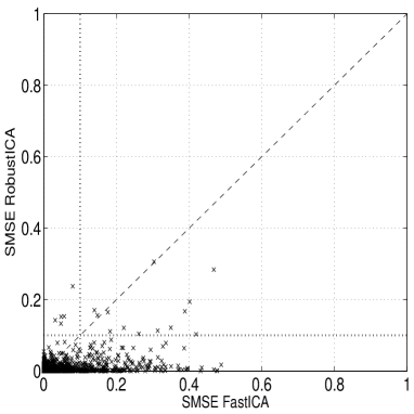
Figure 2: Extraction quality scatter plots for the FastICA and RobustICA algorithms with random orthogonal mixtures of two uniformly distributed sources composed of $T=50$ samples. Termination parameter $\eta=0.5\times 10^{-6}$, 1000 independent trials.

Figure 4: Average extraction quality as a function of computational cost for different sample sizes $T$, with mixture size $K=10$ sources and 1000 mixture realizations. Solid lines: $T=50$. Dashed lines: $T=100$. Dotted lines: $T=150$.

Figure 5: Average extraction quality as a function of block length for different mixture sizes $K$ with complexity fixed at 400 flops/source/sample and 1000 mixture realizations. Solid lines: $K=5$. Dashed lines: $K=10$. Dotted lines: $K=20$.

Figure 6: Average extraction quality in isotropic additive white Gaussian noise with $K=10$ sources, $T$ samples per source and a complexity fixed at 400 flops/source/sample and 1000 mixture realizations. Solid lines: $T=100$. Dashed lines: $T=200$. Dotted lines: $T=500$.

(a)

(b)

Figure 7: Average extraction quality as a function of computational cost for different sample sizes $T$, with mixture size $K=10$ sources and 1000 mixture realizations. Solid lines: $T=50$. Dashed lines: $T=100$. Dotted lines: $T=150$. (a) Without prewhitening. (b) With prewhitening.

Figure 8: Atrial activity extraction in atrial fibrillation ECGs. Top: a 5-second segment of lead V1 from the first patient of the database. Middle: AA contribution to lead V1 estimated by FastICA-SOBI from the 12-lead ECG. Bottom: AA contribution to lead V1 estimated by RobustICA from the 12-lead ECG. Only relative amplitudes are relevant on the vertical axes.

References

- [1] J. Hérault, C. Jutten, and B. Ans, “Détection de grandeurs primitives dans un message composite par une architecture neuromimétique en apprentissage non supervisé,” in Actes 10ème Colloque GRETSI, Nice, France, May 20–24, 1985, pp. 1017–1022.
- [2] P. Comon, “Independent component analysis, a new concept?” Signal Processing, vol. 36, no. 3, pp. 287–314, Apr. 1994, Special Issue on Higher-Order Statistics.
- [3] S. Amari, “Natural gradient works efficiently in learning,” Neural Computation, vol. 10, no. 2, pp. 251–276, Feb. 1998.
- [4] D. T. Pham and P. Garat, “Blind separation of mixture of independent sources through aquasi-maximum likelihood approach,” IEEE Transactions on Signal Processing, vol. 45, no. 7, pp. 1712–1725, July 1997.
- [5] J.-F. Cardoso, “Blind signal separation: statistical principles,” Proceedings of the IEEE, vol. 86, no. 10, pp. 2009–2025, Oct. 1998.
- [6] ——, “Higher-order contrasts for independent component analysis,” Neural Computation, vol. 11, pp. 157–192, 1999.
- [7] P. Comon, “Tensor diagonalization, a useful tool in signal processing,” in Proc. IFAC-SYSID, 10th IFAC Symposium on System Identification, M. Blanke and T. Soderstrom, Eds., vol. 1, Copenhagen, Denmark, July 4–6, 1994, pp. 77–82, invited session.
- [8] R. A. Wiggins, “Minimum entropy deconvolution,” Geoexploration, vol. 16, pp. 21–35, 1978.
- [9] D. Donoho, “On minimum entropy deconvolution,” in Proc. 2nd Applied Time Series Analysis Symposium, Tulsa, OK, 1980, pp. 565–608.
- [10] O. Shalvi and E. Weinstein, “New criteria for blind deconvolution of nonminimum phase systems (channels),” IEEE Transactions on Information Theory, vol. 36, no. 2, pp. 312–321, Mar. 1990.
- [11] N. Delfosse and P. Loubaton, “Adaptive blind separation of independent sources: a deflation approach,” Signal Processing, vol. 45, no. 1, pp. 59–83, July 1995.
- [12] A. Hyvärinen and E. Oja, “A fast fixed-point algorithm for independent component analysis,” Neural Computation, vol. 9, no. 7, pp. 1483–1492, Oct. 1997.
- [13] Z. Ding and T. Nguyen, “Stationary points of a kurtosis maximization algorithm for blind signal separation and antenna beamforming,” IEEE Transactions on Signal Processing, vol. 48, no. 6, pp. 1587–1596, June 2000.
- [14] C. B. Papadias, “Globally convergent blind source separation based on a multiuser kurtosis maximization criterion,” IEEE Transactions on Signal Processing, vol. 48, no. 12, pp. 3508–3519, Dec. 2000.
- [15] J. K. Tugnait, “Identification and deconvolution of multichannel linear non-Gaussian processes using higher order statistics and inverse filter criteria,” IEEE Transactions on Signal Processing, vol. 45, no. 3, pp. 658–672, Mar. 1997.
- [16] A. Hyvärinen, “One-unit contrast functions for independent component analysis: a statistical analysis,” in Proc. IEEE Neural Networks for Signal Processing Workshop, Amelia Island, FL, 1997, pp. 388–397.
- [17] S. Bermejo, “Finite sample effects in higher order statistics contrast functions for sequential blind source separation,” IEEE Signal Processing Letters, vol. 12, no. 6, pp. 481–484, June 2005.
- [18] A. Hyvärinen, “Fast and robust fixed-point algorithms for independent component analysis,” IEEE Transactions on Neural Networks, vol. 10, no. 3, pp. 626–634, May 1999.
- [19] S. Bermejo, “Finite sample effects of the fast ICA algorithm,” Neurocomputing, vol. 71, no. 1-3, pp. 392–399, Dec. 2007.
- [20] A. K. Nandi, Ed., Blind Estimation Using Higher-Order Statistics. Boston, MA: Kluwer Academic Publishers, 1999.
- [21] A. Hyvärinen, J. Karhunen, and E. Oja, Independent Component Analysis. New York: John Wiley & Sons, 2001.
- [22] S. C. Douglas, “On the convergence behavior of the FastICA algorithm,” in Proc. ICA-2003, 4th International Symposium on Independent Component Analysis and Blind Signal Separation, Nara, Japan, Apr. 1–4, 2003, pp. 409–414.
- [23] P. Tichavský, Z. Koldovský, and E. Oja, “Performance analysis of the FastICA algorithm and Cramér-Rao bounds for linear independent component analysis,” IEEE Transactions on Signal Processing, vol. 54, no. 4, pp. 1189–1203, Apr. 2006.
- [24] E. Oja and Z. Yuan, “The FastICA algorithm revisited: convergence analysis,” IEEE Transactions on Neural Networks, vol. 17, no. 6, pp. 1370–1381, Nov. 2006.
- [25] J.-F. Cardoso and A. Souloumiac, “Blind beamforming for non-Gaussian signals,” IEE Proceedings-F, vol. 140, no. 6, pp. 362–370, Dec. 1993.
- [26] P. Comon and E. Moreau, “Improved contrast dedicated to blind separation in communications,” in Proc. ICASSP-97, 22nd IEEE International Conference on Acoustics, Speech and Signal Processing, Munich, Germany, Apr. 21–24, 1997, pp. 3453–3456.
- [27] X. Giannakapoulos, J. Karhunnen, and E. Oja, “An experimental comparison of neural algorithms for independent component analysis and blind separation,” International Journal of Neural Systems, vol. 9, no. 2, pp. 99–114, Apr. 1999.
- [28] P. Chevalier, L. Albera, P. Comon, and A. Ferreol, “Comparative performance analysis of eight blind source separation methods on radiocommunications signals,” in Proc. International Joint Conference on Neural Networks, Budapest, Hungary, July 25–29, 2004.
- [29] Z. Koldovský, P. Tichavský, and E. Oja, “Efficient variant of algorithm FastICA for independent component analysis attaining the cramér-rao lower bound,” IEEE Transactions on Neural Networks, vol. 17, no. 5, pp. 1265–1277, Sept. 2006.
- [30] J.-F. Cardoso, “On the performance of orthogonal source separation algorithms,” in Proc. EUSIPCO-94, VII European Signal Processing Conference, Edinburgh, UK, Sept. 13–16, 1994, pp. 776–779.
- [31] E. Bingham and A. Hyvärinen, “A fast fixed-point algorithm for independent component analysis of complex valued signals,” International Journal of Neural Systems, vol. 10, no. 1, pp. 1–8, Feb. 2000.
- [32] T. Ristaniemi and J. Joutsensalo, “Advanced ICA-based receivers for block fading DS-CDMA channels,” Signal Processing, vol. 82, no. 3, pp. 417–431, Mar. 2002.
- [33] S. C. Douglas, “Fixed-point algorithms for the blind separation of arbitrary complex-valued non-Gaussian signal mixtures,” EURASIP Journal on Advances in Signal Processing, 2007.
- [34] M. Novey and T. Adali, “On extending the complex FastICA algorithm to noncircular sources,” IEEE Transactions on Signal Processing, vol. 56, no. 5, pp. 2148–2154, May 2008.
- [35] ——, “Complex ICA by negentropy maximization,” IEEE Transactions on Neural Networks, vol. 19, no. 4, pp. 596–609, Apr. 2008.
- [36] H. Li and T. Adali, “A class of complex ICA algorithms based on the kurtosis cost function,” IEEE Transactions on Neural Networks, vol. 19, no. 3, pp. 408–420, Mar. 2008.
- [37] E. Moreau and O. Macchi, “A one stage self-adaptive algorithm for source separation,” in Proc. ICASSP-94, 19th IEEE International Conference on Acoustics, Speech and Signal Processing, vol. 3, Adelaide, Australia, Apr. 19–22, 1994, pp. 49–52.
- [38] ——, “Complex self-adaptive algorithms for source separation based on high order contrasts,” in Proc. EUSIPCO-94, VII European Signal Processing Conference, Edinburgh, UK, Sept. 13–16, 1994, pp. 1157–1160.
- [39] V. Zarzoso, P. Comon, and M. Kallel, “How fast is FastICA?” in Proc. EUSIPCO-2006, XIV European Signal Processing Conference, Florence, Italy, Sept. 4–8, 2006.
- [40] V. Zarzoso and P. Comon, “Comparative speed analysis of FastICA,” in Proc. ICA-2007, 7th International Conference on Independent Component Analysis and Signal Separation, London, UK, Sept. 9–12, 2007, pp. 293–300.
- [41] ——, “Robust independent component analysis for blind source separation and extraction with application in electrocardiography,” in Proc. EMBC-2008, 30th Annual International Conference of the IEEE Engineering in Medicine and Biology Society, Vancouver, BC, Canada, Aug. 20–24, 2008, pp. 3344–3347.
- [42] W. H. Press, S. A. Teukolsky, W. T. Vetterling, and B. P. Flannery, Numerical Recipes in C. The Art of Scientific Computing, 2nd ed. Cambridge, UK: Cambridge University Press, 1992.
- [43] A. M. Kuzminskiy, “Automatic choice of the adaption coefficient under nonstationary conditions,” Radioelectronics and Communications Systems, vol. 25, no. 4, pp. 72–74, Apr. 1982.
- [44] ——, “A robust step size adaptation scheme for LMS adaptive filters,” in Proc. DSP’97, 13th International Conference on Digital Signal Processing, vol. 1, Santorini, Greece, July 2–4, 1997, pp. 33–36.
- [45] Y. Huang, J. Benesty, and J. Chen, “Optimal step size of the adaptive multichannel LMS algorithm for blind SIMO identification,” IEEE Signal Processing Letters, vol. 12, no. 3, pp. 173–176, Mar. 2005.
- [46] N. D. Gaubitch, M. Kamrul Hasan, and P. A. Naylor, “Generalized optimal step-size for blind multichannel LMS system identification,” IEEE Signal Processing Letters, vol. 13, no. 10, pp. 624–627, Oct. 2006.
- [47] S. Amari and A. Cichocki, “Adaptive blind signal processing — neural network approaches,” Proceedings of the IEEE, vol. 86, no. 10, pp. 2026–2048, Oct. 1998.
- [48] S. Cruces-Alvarez, A. Cichocki, and S. Amari, “From blind signal extraction to blind instantaneous signal separation: criteria, algorithms, and stability,” IEEE Transactions on Neural Networks, vol. 15, no. 4, pp. 859–873, July 2004.
- [49] L. C. Khor, W. L. Woo, and S. S. Dlay, “Nonlinear blind signal separation with intelligent controlled learning,” IEE Proceedings - Vision, Image and Signal Processing, vol. 152, no. 3, pp. 297–306, June 2005.
- [50] P. A. Regalia, “A finite-interval constant modulus algorithm,” in Proc. ICASSP-2002, 27th International Conference on Acoustics, Speech and Signal Processing, vol. III, Orlando, FL, May 13–17, 2002, pp. 2285–2288.
- [51] P. A. Regalia and E. Kofidis, “Monotonic convergence of fixed-point algorithms for ICA,” IEEE Transactions on Neural Networks, vol. 14, no. 4, pp. 943–949, July 2003.
- [52] V. Zarzoso and P. Comon, “Blind channel equalization with algebraic optimal step size,” in Proc. EUSIPCO-2005, XIII European Signal Processing Conference, Antalya, Turkey, Sept. 4–8, 2005.
- [53] ——, “Semi-blind constant modulus equalization with optimal step size,” in Proc. ICASSP-2005, 30th International Conference on Acoustics, Speech and Signal Processing, vol. III, Philadelphia, PA, Mar. 18–23, 2005, pp. 577–580.
- [54] ——, “Blind and semi-blind equalization based on the constant power criterion,” IEEE Transactions on Signal Processing, vol. 53, no. 11, pp. 4363–4375, Nov. 2005.
- [55] ——, “Optimal step-size constant modulus algorithm,” IEEE Transactions on Communications, vol. 56, no. 1, pp. 10–13, Jan. 2008.
- [56] D. H. Brandwood, “A complex gradient operator and its application in adaptive array theory,” IEE Proceedings F: Communications Radar and Signal Processing, vol. 130, no. 1, pp. 11–16, Feb. 1983.
- [57] D. N. Godard, “Self-recovering equalization and carrier tracking in two-dimensional data communication systems,” IEEE Transactions on Communications, vol. 28, no. 11, pp. 1867–1875, Nov. 1980.
- [58] O. Grellier and P. Comon, “Blind separation of discrete sources,” IEEE Signal Processing Letters, vol. 5, no. 8, pp. 212–214, Aug. 1998.
- [59] “RobustICA package.” [Online]. Available: www.i3s.unice.fr/ zarzoso/robustica.html
- [60] G. H. Golub and C. F. Van Loan, Matrix Computations, 3rd ed. Baltimore, MD: The John Hopkins University Press, 1996.
- [61] V. Zarzoso and P. Comon, “Robust independent component analysis,” I3S Laboratory, University of Nice - Sophia Antipolis, CNRS, Tech. Rep. I3S/RR-2009-02-FR, Mar. 2009. [Online]. Available: http://www.i3s.unice.fr/ mh/RR/2009/RR-09.02-V.ZARZOSO.pdf
- [62] V. Fuster, L. E. Rydén, D. S. Cannom, H. J. Crijns, A. B. Curtis, et al., “ACC/AHA/ESC guidelines for the management of patients with atrial fibrillation – executive summary,” Circulation, vol. 114, no. 7, pp. 700–752, 2006.
- [63] A. Bollmann, D. Husser, L. Mainardi, F. Lombardi, P. Langley, et al., “Analysis of surface electrocardiograms in atrial fibrillation: techniques, research, and clinical applications,” Europace, vol. 8, no. 11, pp. 911–926, 2006.
- [64] F. Castells, J. J. Rieta, J. Millet, and V. Zarzoso, “Spatiotemporal blind source separation approach to atrial activity estimation in atrial tachyarrhythmias,” IEEE Transactions on Biomedical Engineering, vol. 52, no. 2, pp. 258–267, Feb. 2005.
- [65] J. J. Rieta, F. Castells, C. Sánchez, V. Zarzoso, and J. Millet, “Atrial activity extraction for atrial fibrillation analysis using blind source separation,” IEEE Transactions on Biomedical Engineering, vol. 51, no. 7, pp. 1176–1186, July 2004.
- [66] A. Belouchrani, K. Abed-Meraim, J.-F. Cardoso, and E. Moulines, “A blind source separation technique using second-order statistics,” IEEE Transactions on Signal Processing, vol. 45, no. 2, pp. 434–444, Feb. 1997.
- [67] M. G. Jafari and J. A. Chambers, “Fetal electrocardiogram extraction by sequential source separation in the wavelet domain,” IEEE Transactions on Biomedical Engineering, vol. 52, no. 3, pp. 390–400, Mar. 2005.