Simulation of the Laughlin state in an optical lattice

Abstract

We analyze the proposal of achieving a Mott state of Laughlin wave functions in an optical lattice [M. Popp et al., Phys. Rev. A 70, 053612 (2004)] and study the consequences of considering the anharmonic corrections to each single site potential expansion that were not taken into account until now. Our result is that, although the anharmonic correction reduces the maximum frequency at which the system can rotate before the atoms escape from each site (centrifugal limit), the Laughlin state can still be achieved for a small number of particles and a realistic value of the laser intensity.

I Introduction

The fractional quantum Hall effect (FQHE) is one of the most studied phenomena in Condensed Matter Physics Tsui et al. (1982). Despite the fact that a complete understanding of it is still missing, it is commonly believed that the interactions between the particles are essentially responsible for the strange states of matter that the 2D electron gas shows at some particular values of the transverse magnetic field. In this respect, in 1983, Laughlin proposed an Ansatz for the wave function of the ground state of the system Laughlin (1983). This wave function, defined by

$$\Psi_{m}(z_{1},\ldots,z_{N})\sim\prod_{i<j}(z_{i}-z_{j})^{m}e^{-\sum_{i=1}^{N}|z_{i}|^{2}/2}\ ,$$ (1)

where $z_{j}=x_{j}+\textrm{i}y_{j},j=1,\ldots,N$ stands for the position of the $j$-th particle, and $m$ is an integer number, describes the fractional quantum Hall state at a filling fraction $\nu=1/m$. However, this state has only been proven to be an exact eigenstate of very specific Hamiltonians Yoshioka (2002) and for some specific values of the filling fraction; it contains the relevant properties that the ground state of the real system must have.

One of the most important features of some of the fractional quantum Hall states is that they are states of matter whose quasiparticle excitations are neither bosons nor fermions, but particles known as non-Abelian anyons, meaning that they obey non-Abelian braiding statistics. These new phases of matter define a new kind of order in Nature, a topological order Wen (2004). Such systems have become very interesting from the quantum computation perspective. Quantum information could be stored in states with multiple quasiparticles, which would have a topological degeneracy. The unitary gate operations would be simply carried out by braiding quasiparticles, and then measuring the multi-quasiparticle states. In this respect, let us also mention that several spin systems with topological order has been proposed recently as candidates for robust quantum computing Kitaev (2006); Douçot et al. (2005). It has also been shown that these proposals could be implemented by means of cold atoms Duan et al. (2003); Micheli et al. (2006).

Despite the great possibilities of the FQH states, neither the Laughlin wave function nor its anyonic excitations have been observed directly in an experiment so far. Nevertheless, recent experimental advances in the field of ultra-cold atomic gases suggest that they could be good systems to simulate many Condensed Matter phenomena, and, in particular, the FQHE. From the theoretical point of view, it has been shown that the FQH can be realized by rotating a bosonic cloud in a harmonic trap (see Ref. Paredes et al. (2001, 2002)). The rotation plays the role of the magnetic field for the neutral atoms. Thus, in the fast rotation regime, the atoms live in the lowest Landau level and, if a repulsive interaction is introduced, they form the Laughlin wave function. In such system, the Laughlin state is a stable ground state, however, in practice, due to the weak interaction between the particles, the gap is too small, and it is not possible to achieve it experimentally.

An idea to avoid this problem is to use optical lattices Lewenstein et al. (2007); Bloch et al. (2008). In such systems, the interaction energies are larger, since the atoms are confined in a smaller volume. This yields a larger energy gap and, therefore, opens the possibility of achieving FQH states experimentally.

In the present work, we improve the existing proposal of achieving the Laughlin state in an optical lattice presented in Ref. Popp et al. (2004) by studying the consequences of considering not only the harmonic approximation to the single site potential expansion, but also the anharmonic corrections. Our work is organized as follows: first, we analyze the one body Hamiltonian of our system. The solution of the 2D harmonic oscillator is reviewed and a more realistic model for the single site potential of a triangular optical lattice is discussed. Then, we study the many particle problem by introducing a repulsive contact interaction between the particles. We compute, by means of the exact diagonalization technique, the fidelity of the ground state of the system with the Laughlin wave function for a wide range of the experimental parameters. Finally, we discuss which are the required experimental conditions and the procedure to obtain the Laughlin state.

II One body Hamiltonian

II.1 Harmonic case

Let us consider one atom confined in a harmonic potential which rotates in the $x-y$ plane at a frequency $\Omega$. We will assume that the confinement in the $z$ direction is sufficiently strong so that we can ignore the excitations in that direction. The Hamiltonian associated with this system is

$$\hat{H}_{0}^{\prime}=\frac{1}{2M}\left(\hat{p}_{x}^{2}+\hat{p}_{y}^{2}\right)+\frac{1}{2}M\omega^{2}(\hat{x}^{2}+\hat{y}^{2})-\Omega\hat{L},$$ (2)

where $M$ is the mass of the particle, $\hat{p}_{x}$ and $\hat{p}_{y}$ are the canonical momenta associated with the position coordinates $x$ and $y$, $\omega$ is the frequency of the trap and $\hat{L}$ is the angular momentum operator.

We can easily diagonalize this Hamiltonian by defining the creation and annihilation operators of some circular rotation modes $\hat{a}_{\pm}=\frac{1}{\sqrt{2}}\left(\hat{a}_{x}\pm\textrm{i}\hat{a}_{y}\right)$, where $\hat{a}_{x,y}$ are the standard annihilation operators of the 1D harmonic oscillator in the directions $x,y$. In terms of the number operators $\hat{n}_{\pm}\equiv\hat{a}_{\pm}^{\dagger}\hat{a}_{\pm}$ corresponding to these circular creation and annihilation operators, the angular momentum can be written as $\hat{L}=\hbar\left(\hat{n}_{+}-\hat{n}_{-}\right)$ and the Hamiltonian reads

$$\hat{H}_{0}^{\prime}=\hbar\omega(\omega-\Omega)\hat{n}_{+}+\hbar(\omega+\Omega)\hat{n}_{-}+\hbar\omega\,.$$ (3)

Its spectrum is, therefore,

$$E^{0}_{n_{+},n_{-}}=\hbar(\omega-\Omega)n_{+}+\hbar(\omega+\Omega)n_{-}+\hbar\omega\,,$$ (4)

where $n_{\pm}$ are the integer eigenvalues of the number operators $\hat{n}_{\pm}$.

In the fast rotation regime ($\Omega\rightarrow\omega$), the family of states

$$|m\rangle\equiv|n_{+}=m,n_{-}=0\rangle=\frac{1}{\sqrt{m!}}\left(a_{+}^{\dagger}\right)^{m}|0\rangle\,,$$ (5)

where $|0\rangle$ is the state annihilated by both $\hat{a}_{+}$ and $\hat{a}_{-}$, form the subspace of lowest energy, usually known as the lowest Landau Level (LLL). We can write the wave function of these states

$$\varphi_{m}(z)\equiv\langle z|m\rangle=\frac{1}{\sqrt{\pi m!}}z^{m}e^{-\frac{|z|^{2}}{2}}\,,$$ (6)

where $|z\rangle=|x,y\rangle$ are the eigenstates of $\hat{x}$ and $\hat{y}$, $z=\frac{x+\textrm{i}y}{\ell}$ is a complex variable and $\ell=\sqrt{\frac{\hbar}{M\omega}}$ is a characteristic length of the system.

Notice that if the rotation frequency is high but smaller than the trap frequency, the lowest energy subspace is only formed by states with $m<\frac{\omega+\Omega}{\omega-\Omega}$. In this limit, we can find an effective Hamiltonian of our system by projecting the original Hamiltonian onto the LLL,

$$\hat{H_{0}}=\hbar(\omega-\Omega)\hat{L}\,.$$ (7)

Indeed, although Hamiltonians of Eqs. (3) and (7) are different, their projections onto the LLL coincide, $PH_{0}^{\prime}P^{\dagger}=PH_{0}P^{\dagger}$, where $P=\sum_{m}|m\rangle\langle m|$ is the projector onto the LLL.

In Ref. Popp et al. (2004), the formation of fractional quantum Hall states in rotating optical lattices is studied under the approximation of a single particle Hamiltonian as the presented in Eq.  (7). Nevertheless, the potential of a site of an optical lattice is not infinite as the parabolic one. Next, we model in a more realistic way this single site potential and study how it will affect the formation of fractional quantum Hall states.

II.2 Quartic correction

II.2.1 From the lattice potential to our model

We will consider a system of bosonic atoms loaded in a 2D triangular optical lattice Becker et al. (2009). The lattice is 2D due to the confinement in the $x-y$ plane created by two counter propagating lasers in the $z$ direction. In each of this planes a triangular lattice is realized by means of 3 lasers pointing at the directions $\hat{k}_{1}=(\sin\theta,0,\cos\theta)$, $\hat{k}_{2}=(-\sin\theta/2,\sqrt{3}\sin\theta/2,\cos\theta)$ and $\hat{k}_{3}=(-\sin\theta/2,-\sqrt{3}\sin\theta/2,\cos\theta)$, where $\theta$ is the angle between these directions and the $z$ axis.

In the region where the atoms are, the electric field created by each of these lasers can be modeled as a plane wave, $\vec{E}_{j}(\vec{x},t)=A\vec{\epsilon}e^{\textrm{i}(\vec{k}_{j}\cdot\vec{x}-\omega_{L}t)}$, where $\vec{k}_{j}=\frac{2\pi}{\lambda}\hat{k}_{j}$ for $j=1,2,3$ are the wave vectors of the lasers and $\lambda$ is the wavelength of the light used. Notice that all the lasers share the same frequency $\omega_{L}$ and polarization vector $\vec{\epsilon}$. The atoms are subject to the superposition of the electric field $\vec{E}_{i}(\vec{x},t)$ created by each of the lasers,

$$\vec{E}(\vec{x},t)=\sum_{i=1}^{3}\vec{E}_{i}(\vec{x},t)=E(\vec{x})\vec{\epsilon}e^{\textrm{i}\omega_{L}t}.$$ (8)

After averaging over time, the effective potential that atoms feel is, therefore, the correction to the energy of its internal state due to the AC-Stark effect. This energy shift is proportional to the square of the amplitude of the electric field $|E(\vec{x})|^{2}$ and, in our particular case, it can be written as

$$U(\vec{x})=-\frac{2}{9}U_{0}\sum_{\langle i,j\rangle}\cos\left[(\vec{k}_{i}-\vec{k}_{j})\vec{x}\right]\,,$$ (9)

where the sum runs over the 3 different couples of $ij=12,23,31$, and $U_{0}$ is the intensity of the laser. The minima of this potential form a Bravais triangular lattice with basis vectors $\vec{a}_{1}=\frac{2}{3}\frac{\lambda}{\sin\theta}\left(-\frac{1}{2},\frac{\sqrt{3}}{2}\right)$ and $\vec{a}_{2}=\frac{2}{3}\frac{\lambda}{\sin\theta}(1,0)$.

Let us assume that the intensity of the laser $U_{0}\gg E_{R}$, where $E_{R}=\hbar^{2}k^{2}/2M$ is the recoil energy, with $k=2\pi/\lambda$. In this limit, tunneling of atoms between different sites is forbidden, and the lattice can be treated as a system of independent wells. Thus, the ground state of the system is a product state of the state of each site (Mott phase) and we can study the whole system by studying each site of the lattice independently of the others.

In order to describe the potential of a single site, the previous lattice potential in Eq.  (9) is expanded around the equilibrium position $\vec{x}=\vec{0}$,

$$U(\vec{x})\sim\frac{1}{2}M\omega^{2}(x^{2}+y^{2})-\frac{3}{32}k^{4}U_{0}\left(x^{2}+y^{2}\right)^{2}+O(x^{6})\,.$$ (10)

We get a harmonic oscillator term with frequency $\omega=2\sqrt{U_{0}E_{R}}/\hbar$ plus a quartic perturbation and higher order corrections. Notice that both terms of the expansion respect the rotational symmetry. This is actually the reason why we have considered a triangular lattice instead of the simpler square one. In the square lattice, the circular symmetry is broken in fourth order of the expansion, while in the triangular one, this does not happen until the sixth order. From now on, it will be considered that our single site potential is adequately described by only these harmonic and quartic terms of the expansion of the potential. This approximation is reasonable since it has already been assumed $U_{0}\gg E_{R}$.

Furthermore, by introducing some phase modulators into the lasers that form the lattice, it is possible to create time averaged potentials that generate an effective rotation of the single lattice sites. If this rotation $\Omega$ is close to $\omega$, the system is in the fast rotation regime and we can obtain the low energy Hamiltonian proceeding as before. Written in units of $\hbar\omega$, it becomes

$$\hat{H}=\hbar\left(1-\frac{\Omega}{\omega}\right)\hat{L}-\gamma\left(\frac{\hat{x}^{2}+\hat{y}^{2}}{\ell^{2}}\right)^{2}\,,$$ (11)

where $\gamma\equiv\frac{3}{32}\frac{U_{0}k^{4}\ell^{4}}{\hbar\omega}=\frac{3}{64}\sqrt{\frac{E_{R}}{U_{0}}}$ is a perturbation parameter. Notice that the perturbation parameter, $\gamma$, only depends on the intensity of the laser in units of the energy recoil.

In summary, we have described the whole sophisticated optical lattice by a set of independent wells modeled by the simple Hamiltonian presented in Eq.  (11). This effective Hamiltonian is the same from Eq.  (7) plus a quartic correction term which will be responsible for all the new physics that are going to be studied next.

II.2.2 Exact solution

Next, we find the lowest energy eigenstates of the Hamiltonian presented in Eq.  (11). First of all, we realize that both $H$ and $H_{0}$ are rotationally invariant, therefore, $[H,H_{0}]=[H,L]=0$. Thus, $H,H_{0}$ and $L$ must have a common eigenbasis, and this can only be $\{|m\rangle\}$. We determine the eigenvalues of $H$ by computing the expected values

$$E_{m}=\langle m|H|m\rangle=\left(1-\frac{\Omega}{\omega}\right)m-\gamma(m+1)(m+2)\,,$$ (12)

in units of $\hbar\omega$.

Let us point out that the commutator between the Hamiltonians of the harmonic and anharmonic systems before being projected onto LLL, $[H^{\prime},H_{0}^{\prime}]$, is not zero. Therefore, their lowest energy eigenstates only coincide in the fast rotation regime.

It is important, then, to establish which is the fast rotation regime for the Hamiltonian (11) or, in other words, under which conditions our low energy description of the system is correct. To see this, we can compute, using perturbation theory, the first correction to the energy of the second Landau level (NL) states

$$E_{m}^{NL}=(m+2)-\gamma(m+7)(m+2)\,.$$ (13)

We realize that the LLL is a good description of the lowest energy states, i. e. $E_{m}\ll E_{m}^{NL}$, if $3\gamma(m+1)\ll 1$. In this regime, the projection of the Hamiltonian onto the LLL is a good effective description of our system. From now on, this condition will be always assumed.

II.3 Maximum rotation frequency

In the harmonic case, we realize that if the rotating frequency $\Omega$ exceeds the frequency of the trap $\omega$ (see Eq.  (7)), the lower energy states have an infinite angular momentum, i. e. all the particles of the system are expelled from the trap. This maximum frequency is usually known as the centrifugal limit. What we are going to study now is, therefore, how the introduction of the quartic perturbation will affect the centrifugal limit of the system. In order to answer this question we realize two different analysis that give quite similar results.

The first argument consists of a semi-classical interpretation of the dynamics of the particle. In the anharmonic system, we have a competition between the attractive force of the harmonic trap and the repulsive forces corresponding to the quartic correction and the fictitious centrifugal force. In the central region, the harmonic trap dominates and the particles are confined, while if a particle was in the exterior region, it would be expelled. The limit radius between these two regions corresponds to the maximum of the effective potential that includes both the trap and centrifugal terms. Furthermore, from the semi-classical point of view, each stationary state $|m\rangle$ follows a circular trajectory of radius $r\sim\sqrt{m}$ around the origin. We expect then that those states whose associated radius is less than the limit radius are bound states. Thus, we find that the maximum rotation frequency, or the centrifugal limit, depends on the maximum angular momentum that we want to keep in the trap. This is a remarkable difference with respect to the harmonic case, where the centrifugal limit was the same for any angular momentum state. In particular and according to this semi-classical criterion, the centrifugal limit for a particle with an angular momentum equal or less than $m_{L}$ is

$$\Omega_{L}=\omega\sqrt{1-4\gamma m_{L}}\simeq\omega(1-2\gamma m_{L})\,.$$ (14)

Figure 1: Spectra of the single-particle Hamiltonian shown in Eq. (11) that models the dynamics of a particle in a rotating single site of a triangular optical lattice. This plot has been realized for $\gamma=0.01$ and $\Omega=0.8\omega$. Notice that for these particular values of the frequency rotation and the laser intensity, particles with an angular momentum larger than $m_{L}=8$ would be expelled.

Another approach is to think in terms of the slope of the spectra $E_{m}$ presented in Eq.  (12) and plotted in Fig. 1. We realize that the single particle energy $E_{m}$ begins growing with $m$ from $m=0$, reaches a maximum at $\left[\frac{1-\Omega/\omega-3\gamma}{2\gamma}+\frac{1}{2}\right]$, (where the brackets $[$ $]$ represent the integer part function), and becomes monotonically decreasing from this point. We interpret this in the same way as the harmonic case, that is to say, those states $|m\rangle$ that are in an energy interval with a negative slope are unstable. According to this interpretation, the angular momentum of a particle must be less than $\left[\frac{1-\Omega/\omega-3\gamma}{2\gamma}+\frac{1}{2}\right]$ in order to be trapped. This implies that the centrifugal limit for a trapped particle with angular momentum $m_{L}$ is

$$\Omega_{L}=\omega(1-2\gamma m_{L}-4\gamma)\,.$$ (15)

Although the previous approaches are different, notice that they predict practically the same centrifugal limit. In our simulations presented in Sec. IV, we have taken the condition given by Eq.  (15), since it is the most restrictive one.

At this point, we have completely solved the one particle problem. Let us note that whereas in the harmonic case the maximum rotation frequency coincides always with the trap frequency, in the system with the quartic perturbation, this centrifugal limit depends on which is the maximum angular momentum of a particle that we want to keep trapped. This difference will be crucial to understand why it will be more difficult to obtain the Laughlin state in the anharmonic case than in the harmonic one.

III Many particle problem

The Laughlin state is a strongly correlated state, therefore, interaction between atoms will play an essential role in its experimental realization.

Let us consider, then, a set of $N$ bosons trapped in a well as the one described previously, and interacting by means of a repulsive contact potential,

$$V(\vec{r}-\vec{r}^{\prime})=g\delta(\vec{r}-\vec{r}^{\prime})\,,$$ (16)

where the parameter $g$ accounts for the strength of the interaction, and is related to the s-wave scattering length, $a_{s}$, and to the localization length in the $z$ direction, $\ell_{z}$, by $g=\sqrt{\frac{2}{\pi}}\frac{a_{s}}{\ell_{z}}$.

We are interested in knowing the ground state of the system for a wide range of $g$ and $U_{0}/E_{R}$ in order to see under which conditions the Laughlin state could be realized experimentally. The solution of this problem is trivial in the extreme cases $g\to 0$ and $g\to\infty$.

When $g=0$, the atoms do not interact and the ground state of the system is merely a product state with all the atoms with angular momentum zero.

If $g\to\infty$, the atoms will find a configuration in which they are always in a different position with the minimum total angular momentum possible. This configuration that minimizes the interaction energy at the expense of the angular momentum of the particles is precisely the Laughlin state. As we can see in Eq.  (1), the interaction energy in the Laughlin wave function is strictly zero since the probability that two atoms are in the same position is null.

For a finite $g$, the problem of finding the ground state of the system has to be addressed numerically. In particular, we will solve it by means of exact diagonalization. With this aim, we can write the Hamiltonian of this system in second quantization form,

$$\hat{H} =\sum_{j=1}^{L}\left((1-3\gamma-\Omega)\hat{n}_{i}-\gamma\hat{n}_{i}^{2}+1-2\gamma\right)$$

$$+\frac{1}{2}\sum_{i<j}V_{ijkl}b_{i}b_{j}b_{k}^{\dagger}b_{l}^{\dagger}\,,$$ (17)

where $b_{j}$ and $b_{j}^{\dagger}$ are the creation and annihilation operators of the mode $j$ which corresponds to the LLL state with angular momentum $j$ presented in Eq.  (6), $\hat{n}_{j}\equiv b_{j}^{\dagger}b_{j}$ counts the number of particles with angular momentum $j$, and $V_{ijkl}$ are the coefficients of the interaction in this basis defined by

$$V_{m_{1}\,m_{2}\,m_{3}\,m_{4}} =\langle m_{1}\,m_{2}|\hat{V}|m_{3}\,m_{4}\rangle$$ (18)

$$=\frac{g}{2\pi}\,\,\frac{\delta_{m_{1}+m_{2},m_{3}+m_{4}}}{\sqrt{m_{1}!m_{2}!m_{3}!m_{4}!}}\,\,\frac{(m_{1}+m_{2})!}{2^{m_{1}+m_{2}}}\>.$$

The cylindrical symmetry of the Hamiltonian allows the diagonalization to be performed in different subspaces of well defined total $z$-component of $L=\sum_{i=1}^{N}m_{i}$.

Thus, given the parameters $\Omega,U_{0}/E_{R}$ and $g$ and a subspace of total angular momentum $L$, we construct the multi-particle basis of $N$ particles compatible with $L$, calculate the matrix-elements of the Hamiltonian in this subspace by means of Eq.  (17), and perform its diagonalization. Once the ground state for each subspace $L$ is determined, we find the ground state of the system by selecting the state with lowest energy.

An important issue that we have to take into account when we perform the simulation is to be careful with the centrifugal limit. As it has been shown in Sec. II.3, if we want that the particle with the maximum angular momentum does not escape from the trap, we have to keep the rotation below the centrifugal limit given by Eq.  (15). In our case, in which we want to drive the system into the Laughlin state, this centrifugal limit is determined by the maximum angular momentum of a single particle in the Laughlin state, that is $N(N-1)/2$. Thus, the maximum rotation frequency is given by Eq.  (15) taking

$$m_{L}=N(N-1)/2\,.$$ (19)

IV Results and discussion

In what follows, we display the results obtained from exact diagonalization described in the previous section.

In order to study under which conditions the Laughlin state is the ground state of the system a phase diagram is presented in Fig. 2. The fidelity between the Laughlin state and the GS of the system is plotted versus the laser intensity $U_{0}/E_{R}$ and the strength of the contact interaction $g$. For each value of $U_{0}/E_{R}$, we have taken the maximum possible rotation frequency, defined by Eq.  (15), since it corresponds to the best condition to achieve the Laughlin wave function. The plot shows two separated phases. In one of them, the Laughlin state is perfectly obtained ($\langle GS|\Psi_{L}\rangle=1$). It corresponds to high values of the laser intensity and strength of the interaction. On the contrary, for low values of $U_{0}/E_{R}$ and $g$ the fidelity between the GS and the Laughlin state is zero. This phase corresponds to other states with less angular momenta and not so correlated.

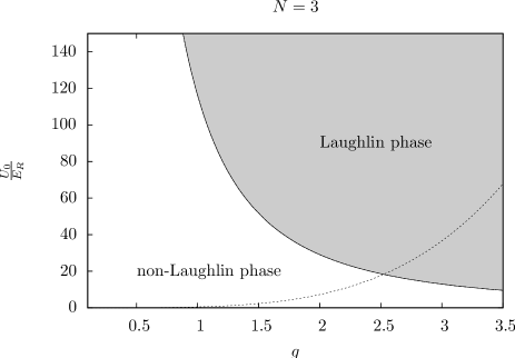
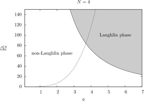
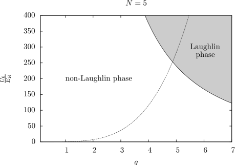
Figure 2: Density plot of the fidelity between the GS of the system and the Laughlin wave function versus the laser intensity $U_{0}$ and the strength of the contact interaction $g$ for different number of particles ($N$=3,4 and 5). In order to realize the diagram, the maximum possible rotation frequency $\Omega_{L}$ has been considered for each value of $U_{0}$. The dashed line represents the dependence of $g$ on the confinement $U_{0}$ for the Rubidium atoms case. Although the $U_{0}$ needed to get the Laughlin as the ground state of the system increases enormously with the number of particles, we realize that for small values of $N$, the laser intensity required is achievable.

Notice that the transition between the Laughlin and non-Laughlin phases is very abrupt. This is because the ground state in the non-Laughlin phase has an angular momentum smaller than the angular momentum that Laughlin state requires. States with different angular momentum are orthogonal and therefore the fidelity between them is zero. Nevertheless, when interaction is high enough and it is sufficiently favorable for the system to have total angular momentum $L=N(N-1)$, the Laughlin wave function is instantly achieved. This argument is illustrated in Fig. 3 for the case of $N=4$ particles. We can see how the system increases its angular momentum depending on the confinement $U_{0}$ and the interaction $g$.

In Fig. 2, the shape of the boundary between the Laughlin and non-Laughlin phases can be easily explained. According to the argument presented in the previous section, the configuration of the ground state of the system depends on the ratio between the strength of the interaction $g$ and the energy difference of the single particle spectrum $\Delta E\equiv E_{m_{L}}-E_{0}=\gamma m_{L}(m_{L}+1)$ (see Fig. 1). In particular, we expect two regimes:

• If $g\gg\Delta E$, the GS is the Laughlin state,

• while if $g\ll\Delta E$, then GS is a product state with all the particles with angular momentum 0.

The transition, then, takes place between these two regimes, that is, when $g\sim\Delta E$. This condition implies that

$$g=f(N)\sqrt{\frac{E_{R}}{U_{0}}}$$ (20)

where $f(N)\sim m_{L}(m_{L}+1)$ is a function that depends on $N$.

In Fig. 4, we plot the numerical data $(\sqrt{\frac{E_{R}}{U_{0}}},g)$ corresponding to the points of the border between the Laughlin and non-Laughlin phases of Fig. 2 for $N=4$ in order to see if Eq. (20) is fulfilled. We observe a perfect fit between numerical data and Eq. (20) and, performing a linear regression, we determine the slope $f(4)=33.876(1)$. The same perfect agreement has been found for $N=3$ and $N=5$ cases, with slopes $f(3)=10.779(1)$ and $f(5)=77.427(3)$ respectively.

According to Eq. (20), we would expect that function $f(N)$ scales as $\sim N(N-1)\left(N(N-1)+2\right)$. Nevertheless, although $f(3)$, $f(4)$ and $f(5)$ seem to scale in this way, three points are not enough to confirm this behavior.

Figure 3: Density plot of the angular momentum of the GS of the system respect to the laser intensity $U_{0}$ and the strength of the contact interaction $g$ for $N$=4. In order to realize the diagram, the maximum possible rotation frequency $\Omega_{L}$ has been considered for each value of $U_{0}$.

Figure 4: Plot of the points $(\sqrt{\frac{E_{R}}{U_{0}}},g)$ of the border between the two phases Laughlin and non-Laughlin of Fig. 2 for $N=4$. We realize that Eq. 20 describes perfectly its behavior.

The dashed line in Fig. 2 expresses the dependence of $g$ on the confinement $U_{0}$ for the Rubidium atoms case (see Eq.  (21)). It shows the natural path that the system would follow increasing the intensity of the laser without improving the strength of the interaction by means of Feshbach resonance techniques. This illustrates the advantages of confining ultra-cold gases in an optical lattice. The high confinement increases the scattering length of the interaction between the atoms,

$$g=\sqrt{2}a_{s}|k|\left(\frac{U_{0}}{E_{R}}\right)^{1/4}\,,$$ (21)

which, at the end of the day, is responsible for the high correlation of the GS.

Moreover, this enhanced interaction produces a larger energy gap which makes the optical lattice proposal more robust compared to the harmonic trap setup. This enhancement in the energy gap of the excitation spectrum can alleviate some of the challenges for experimental realization of the quantum Hall state for ultra-cold atoms.

In Fig. 2, we also realize that the larger the number of atoms of the system is, higher the laser intensity needed to achieve the Laughlin state. The reason for this is that for larger $N$, the maximum angular momenta allowed before the atoms escape from the trap is larger, $m_{L}=N(N-1)/2$. This implies a smaller maximum rotation frequency $\Omega_{L}$ (see Eq. (15)), and the requirement of increasing the laser intensity $U_{0}$ to compensate this effect. Let us note that increasing $U_{0}$ we achieve both larger maximum rotation frequency and a stronger interaction $g$.

It is interesting to point out that driving the system into the Laughlin wave function is not possible by simply increasing the rotation frequency, since the symmetric shape of the potential conserves the angular momenta and the system would rest in a trivial non-entangled state with angular momentum zero. To avoid this, we should introduce some deformation to the wells of the lattice in order to break the spherical symmetry. For our optical lattice setup this can be achieved by introducing a couple of electro-optical fast phase modulators whose effect in the rotating frame would be a new trapping potential with the form $V_{p}\propto\left(\omega+\Delta\omega\right)^{2}x^{2}+\omega^{2}y^{2}$. This modification would change our original Hamiltonian in a new one $H+H_{\epsilon}$, where

$$H_{\epsilon}=\frac{\epsilon}{4}\sum_{m}\beta_{m}b_{m+2}^{\dagger}b_{m}+(m+1)b_{m}^{\dagger}b_{m}+\textrm{h.c.},$$ (22)

where $\beta_{m}=\sqrt{(m+2)(m+1)}$ and $\epsilon=\Delta\omega/\omega$ is a small parameter.

The previous perturbation (22) leads to quadrupole excitations, so that states whose total angular momentum differ by two units are coupled, and the system can increase its angular momentum. In order to drive the system into the Laughlin state, we could follow some adiabatic paths in the parameter space ($\Omega$, $\epsilon$) such that the gap along this paths is as large as possible, and in this way, keep the system in its ground state according to the adiabatic theorem Born and Fock (1928).

Finally, let us briefly discuss how to check that we have driven the system to the Laughlin state. First, notice that as the system is in a Mott phase, any measurement signal will be enhanced by a factor equal to the number of occupied lattice sites.

According to Ref. Read and Cooper (2003), for any LLL state of a trapped, rotating, interacting Bose gas, the particle distribution in coordinate space in a time of flight experiment is related to that in the trap at the time it is turned off by a simple rescaling and rotation. Thus, it is possible to measure the density profile of our state by accomplishing a time of flight experiment. Notice that by means the density profile it is possible to estimate the total angular momentum of the system.

Although the angular momentum of the system can be measured, there are many states with the same angular momentum that are not the Laughlin state. Thus, in order to really distinguish if the system is in the Laughlin state, the measurement of other properties is required. One possibility is the measurement of correlations. In Ref. Popp et al. (2004), an interesting technique is proposed to measure the correlation functions $g_{1}=\langle\psi^{\dagger}({\bf r})\psi({\bf r^{\prime}})\rangle$ and $g_{2}=\langle\psi^{\dagger}({\bf r})\psi^{\dagger}({\bf r^{\prime}})\psi({\bf r})\psi({\bf r^{\prime}})\rangle$. These functions are very particular for the Laughlin state. For instance, $g_{2}\propto\lvert r-r^{\prime}|^{4}$, since in the Laughlin state all the particles have a relative angular momentum $m_{r}=2$ between them. Let us just mention the scheme of this technique. It lies in using a gas of two species that can be coupled via Raman transitions (hyperfine levels). First, all the atoms are in the same state and the system is driven to the Laughlin state. Then, an equal superposition of the two species is created by means of a $\pi/2$-pulse with the laser. Next, the atoms are shifted a small distance compared to the lattice spacing by moving the lattice of one of the species (as was proposed in Ref. Jaksch et al. (2000) and experimentally realized in Ref. Mandel et al. (2003)). Finally, another $\pi/2$-pulse is performed in order to put all the atoms in the same state and the time of flight measurement is accomplished.

V Conclusions

The method for achieving the Laughlin state in an optical lattice presented in Ref. Popp et al. (2004) has been studied. It has been shown that it is essential to take into account the anharmonic corrections. A quartic anharmonic term introduces a maximum rotation frequency that is smaller than in the harmonic case and, therefore, if this was not considered all the particles would be expelled from their single lattice sites.

Although this more restrictive centrifugal limit makes more difficult to drive the system into the Laughlin state, since it requires higher values of $U_{0}$, for systems with a small number of particles, the Laughlin state is achievable experimentally.

The shape of the boundary between the Laughlin and non-Laughlin phases in the phase diagram of the system respect to the confinement $U_{0}$ and the strength of the interaction $g$ plotted in Fig. 2 has been physically explained and analytically described.