Two-loop renormalization of fermion bilinear operators on the lattice

Abstract:

We compute the renormalization functions on the lattice, in the $RI^{\,\prime}$ scheme, of local bilinear quark operators $\bar{\psi}\Gamma\psi$, where $\Gamma=\hat{1},\,\gamma_{5},\,\gamma_{\mu},\,\gamma_{5}\,\gamma_{\mu},\,\gamma_{5}\,\sigma_{\mu\,\nu}$. This calculation is carried out to two loops for the first time. We consider both the flavor non-singlet and singlet operators.

As a prerequisite for the above, we compute the quark field renormalization, $Z_{\psi}^{L,RI^{\,\prime}}$, up to two loops. We also compute the 1-loop renormalization functions for the gluon field, $Z_{A}^{L,RI^{\,\prime}}$, ghost field, $Z_{c}^{L,RI^{\,\prime}}$, gauge parameter, $Z_{\alpha}^{L,RI^{\,\prime}}$, and coupling constant $Z_{g}^{L,RI^{\,\prime}}$.

We use the clover action for fermions and the Wilson action for gluons. Our results are given as an explicit function of the coupling constant $a_{\circ}=g_{\circ}^{2}/16\pi^{2}$, the clover coefficient $c_{SW}$, and the number of fermion colors ($N_{c}$) and flavors ($N_{f}$), in the renormalized Feynman gauge. All 1-loop quantities are evaluated in an arbitrary gauge.

Finally, we present our results in the $\overline{MS}$ scheme, for easier comparison with calculations in the continuum. We have generalized to fermionic fields in an arbitrary representation. Some special features of superficially divergent integrals, obtained from the evaluation of two-loop Feynman diagrams, are presented in detail in Ref. [1].

1 Introduction

Numerical simulations of QCD, formulated on the lattice, make use of a variety of composite operators, made out of quark fields. Matrix elements and correlation functions of a whole variety of such operators, are computed in order to study hadronic properties in this context. A proper renormalization of these operators is essential for the extraction of physical results from the lattice.

In this work we study the renormalization function, $Z_{\Gamma}$, of fermion bilinears ${\cal O}=\bar{\psi}\Gamma\psi$ on the lattice, where $\Gamma=\hat{1},\,\gamma_{5},\,\gamma_{\mu},\,\gamma_{5}\,\gamma_{\mu},\,\gamma_{5}\,\sigma_{\mu\,\nu}$ ($\sigma_{\mu\,\nu}=1/2\,[\gamma_{\mu},\gamma_{\nu}]$). We consider both flavor singlet and nonsinglet operators. We employ the standard Wilson action for gluons and clover-improved Wilson fermions. The number of quark flavors $N_{f}$, the number of colors $N_{c}$ and the clover coefficient $c_{{\rm SW}}$ are kept as free parameters. One necessary ingredient for the renormalization of fermion bilinears is the 2-loop quark field renormalization, $Z_{\psi}$, calculated in [2]. The one-loop expression for the renormalization function $Z_{g}$ of the coupling constant is also necessary for expressing the results in terms of both the bare and the renormalized coupling constant.

Our two-loop calculations have been performed in the bare and in the renormalized Feynman gauge. For the latter, we need the 1-loop renormalization functions $Z_{\alpha}$ and $Z_{A}$ of the gauge parameter and gluon field respectively, as well as the one-loop expressions for $Z_{\Gamma}$ with an arbitrary value of the gauge parameter.

The main results presented in this work are 2-loop bare Green’s functions (amputated, one-particle irreducible (1PI)), for the scalar, pseudoscalar, vector, axial vector and tensor operator, as functions of the lattice spacing, $a_{{}_{\rm L}}$, and the external momentum $q$. In general, one can use bare Green’s functions to construct $Z_{{\cal O}}^{X,Y}$, the renormalization function for operator ${\cal O}$, computed within a regularization $X$ and renormalized in a scheme $Y$. We employ two widely used schemes to compute the various 2-loop renormalization functions: The $RI^{\prime}$ scheme and the $\overline{MS}$ scheme.

The present work is the first two-loop computation of the renormalization of fermion bilinears on the lattice. One-loop computations of the same quantities exist for quite some time now (see, e.g., [3] and references therein). There have been made several attempts to estimate $Z_{{\cal O}}$ non-perturbatively; recent results can be found in Refs. [4, 5, 6]. A series of results have also been obtained using stochastic perturbation theory [7]. A related computation, regarding the fermion mass renormalization $Z_{m}$ with staggered fermions, can be found in [8].

2 Formulation of the problem

We will make use of the Wilson formulation of the QCD action on the lattice, with the addition of the clover (SW) term for fermions. In standard notation, it reads:

$$S_{L} = S_{G}+\sum_{f}\sum_{x}(4r+m_{\rm o})\bar{\psi}_{f}(x)\psi_{f}(x)$$

$$- {1\over 2}\sum_{f}\sum_{x,\,\mu}\bigg{[}\bar{\psi}_{f}(x)\left(r-\gamma_{\mu}\right)U_{x,\,x+\mu}\,\psi_{f}(x+{\mu})+\bar{\psi}_{f}(x+{\mu})\left(r+\gamma_{\mu}\right)U_{x+\mu,\,x}\,\psi_{f}(x)\bigg{]}$$

$$- {1\over 4}\,c_{\rm SW}\,\sum_{f}\sum_{x,\,\mu,\,\nu}\bar{\psi}_{f}(x)\,\sigma_{\mu\nu}\,{\hat{F}}_{\mu\nu}(x)\,\psi_{f}(x),$$

$${\rm where:}\ {\hat{F}}_{\mu\nu} \equiv {1\over{8a^{2}}}\,(Q_{\mu\nu}-Q_{\nu\mu})$$ (2)

$${\rm and:}\ Q_{\mu\nu} = U_{x,\,x+\mu}\,U_{x+\mu,\,x+\mu+\nu}\,U_{x+\mu+\nu,\,x+\nu}\,U_{x+\nu,\,x}+U_{x,\,x+\nu}\,U_{x+\nu,\,x+\nu-\mu}\,U_{x+\nu-\mu,\,x-\mu}\,U_{x-\mu,\,x}$$ (3)

$$+ U_{x,\,x-\mu}\,U_{x-\mu,\,x-\mu-\nu}\,U_{x-\mu-\nu,\,x-\nu}\,U_{x-\nu,\,x}+U_{x,\,x-\nu}\,U_{x-\nu,\,x-\nu+\mu}\,U_{x-\nu+\mu,\,x+\mu}\,U_{x+\mu,\,x}\qquad\,$$

$S_{G}$ is the standard pure gluon action, made out of $1{\times}1$ plaquettes. $r$ is the Wilson parameter (set to $r=1$ henceforth); $f$ is a flavor index. Powers of the lattice spacing $a_{{}_{\rm L}}$ have been omitted and may be directly reinserted by dimensional counting.

The “Lagrangian mass” $m_{\rm o}$ is a free parameter in principle. However, since we will be using mass independent renormalization schemes, all renormalization functions which we will be calculating, must be evaluated at vanishing renormalized mass, that is, when $m_{\rm o}$ is set equal to the critical value $m_{\rm cr}$: $m_{\rm o}\to m_{\rm cr}=m_{1}\,g_{\circ}^{2}+{\cal O}(g_{\circ}^{4})$.

One prerequisite to our programme consists of the renormalization functions, $Z_{A}$, $Z_{c}$, $Z_{\psi}$, $Z_{g}$ and $Z_{\alpha}$, for the gluon, ghost and fermion fields ($A_{\mu}^{a},\ c^{a},\ \psi$), and for the coupling constant $g$ and gauge parameter $\alpha$, respectively (for definitions of these quantities, see Ref. [2]); we will also need the fermion mass counterterm $m_{\rm cr}$. These quantities are all needed to one loop, except for $Z_{\psi}$ which is required to two loops. The value of each $Z_{{\cal O}}$ depends both on the regularization $X$ and on the renormalization scheme $Y$ employed, and thus should properly be denoted as $Z^{X,Y}_{{\cal O}}$.

As mentioned before, we employ the $RI^{\prime}$ renormalization scheme [9], which is more immediate for a lattice regularized theory. It is defined by imposing a set of normalization conditions on matrix elements at a scale $\bar{\mu}$, where (just as in the $\overline{MS}$ scheme):

$$\bar{\mu}=\mu\,(4\pi/e^{\gamma_{{}_{\,\rm E}}})^{1/2}$$ (4)

where $\gamma_{{}_{\,\rm E}}$ is the Euler constant and $\mu$ is the scale entering the bare coupling constant $g_{\circ}=\mu^{\epsilon}\,Z_{g}\,g$ when regularizing in $D=4-2\epsilon$ dimensions.

3 Renormalization of fermion bilinears

The lattice operators ${\cal O}_{\Gamma}=\bar{\psi}\,\Gamma\,\psi$ must, in general, be renormalized in order to have finite matrix elements. We define renormalized operators by

$${\cal O}^{RI^{\prime}}_{\Gamma}=Z^{L,RI^{\prime}}_{\Gamma}(a_{{}_{\rm L}}\bar{\mu})\,{\cal O}_{\Gamma\,{\rm o}}$$ (5)

The renormalization functions $Z_{\Gamma}^{L,RI^{\prime}}$ can be extracted through the corresponding bare 2-point functions $\Sigma^{L}_{\Gamma}(qa_{{}_{\rm L}})$ (amputated, 1PI) on the lattice, through the employment of the $RI^{\prime}$ renormalization conditions:

$$\lim_{a_{{}_{\rm L}}\rightarrow 0}\left[Z_{\psi}^{L,RI^{\,\prime}}\,Z_{\Gamma}^{L,RI^{\,\prime}}\,\Sigma^{L}_{\Gamma}(qa_{{}_{\rm L}})\right]_{q^{2}=\bar{\mu}^{2}}=\Gamma_{\rm tree},$$ (6)

where $\Sigma^{L}_{\Gamma}(qa_{{}_{\rm L}})$ is the appropriate bare 1PI 2-point Green’s function on the lattice and $\Gamma_{\rm tree}$ is its tree-level value. For the vector (V), axial-vector (AV) and tensor (T) operators, we can express the bare Green’s functions in the following way:

$$\Sigma^{L}_{V}(qa_{{}_{\rm L}}) = \gamma_{\mu}\,\Sigma^{(1)}_{V}(qa_{{}_{\rm L}})+\frac{q^{\mu}{/}\mskip-10.0muq}{q^{2}}\Sigma^{(2)}_{V}(qa_{{}_{\rm L}})$$

$$\Sigma^{L}_{AV}(qa_{{}_{\rm L}}) = \gamma_{5}\gamma_{\mu}\,\Sigma^{(1)}_{AV}(qa_{{}_{\rm L}})+\gamma_{5}\frac{q^{\mu}{/}\mskip-10.0muq}{q^{2}}\Sigma^{(2)}_{AV}(qa_{{}_{\rm L}})$$ (7)

$$\Sigma^{L}_{T}(qa_{{}_{\rm L}}) = \gamma_{5}\,\sigma_{\mu\,\nu}\Sigma^{(1)}_{T}(qa_{{}_{\rm L}})+\gamma_{5}\frac{{/}\mskip-10.0muq\,(\gamma_{\mu}q_{\nu}-\gamma_{\nu}q_{\mu})}{q^{2}}\Sigma^{(2)}_{T}(qa_{{}_{\rm L}})$$

Only the $\Sigma^{(1)}_{V,\,AV,\,T}(qa_{{}_{\rm L}})$ parts are involved in Eq. (6). It is worth noting here that terms which break Lorentz invariance (but are compatible with hypercubic invariance), such as $\gamma_{\mu}\,(q^{\mu})^{2}/q^{2}$, turn out to be absent from all bare Green’s functions; thus, the latter have the same Lorentz structure as in the continuum.

For easier comparison with calculations coming from the continuum, we need to express our results in the $\overline{MS}$ scheme. For each renormalization function on the lattice, $Z^{L,RI^{\prime}}_{{\cal O}}$, we can construct its $\overline{MS}$ counterpart using conversion factors:

$$C_{\Gamma}(g,\alpha)\equiv\frac{Z_{\Gamma}^{L,RI^{\prime}}}{Z_{\Gamma}^{L,\overline{MS}}}=\frac{Z_{\Gamma}^{DR,RI^{\prime}}}{Z_{\Gamma}^{DR,\overline{MS}}}$$ (8)

These conversion factors are regularization independent; thus they can be calculated more easily in dimensional (DR), rather than Lattice (L), regularization, (see, e.g., Ref. [10]). Due to the non-unique generalization of $\gamma_{5}$ to D dimensions, the pseudoscalar and axial-vector bilinear operators require special attention in the $\overline{MS}$ scheme.

For a more detailed analysis of the renormalization of fermion bilinears and their conversion to the $\overline{MS}$ scheme, see Refs. [1, 2].

4 Computation and Results

The Feynman diagrams contributing to the bare Green’s functions, at 1- and 2-loop level, are shown in Figs. 1 and 2, respectively. For flavor singlet bilinears, there are 4 extra diagrams, shown in Fig. 3, which contain the operator insertion inside a closed fermion loop. These diagrams give a nonzero contribution only in the scalar and axial-vector cases.

Figure 1: One-loop diagram contributing to $Z_{\Gamma}$. A wavy (solid) line represents gluons (fermions). A cross denotes the Dirac matrices $\hat{1}$ (scalar), $\gamma_{5}$ (pseudoscalar), $\gamma_{\mu}$ (vector), $\gamma_{5}\gamma_{\mu}$ (axial vector) and $\gamma_{5}\sigma_{\mu\nu}$ (tensor).

Figure 2: Two-loop diagrams contributing to $Z_{\Gamma}$. Wavy (solid, dotted) lines represent gluons (fermions, ghosts). A solid box denotes a vertex from the measure part of the action; a solid circle is a mass counterterm; crosses denote the Dirac matrices $\hat{1}$ (scalar), $\gamma_{5}$ (pseudoscalar), $\gamma_{\mu}$ (vector), $\gamma_{5}\gamma_{\mu}$ (axial-vector) and $\gamma_{5}\sigma_{\mu\nu}$ (tensor).

Figure 3: Extra two-loop diagrams contributing to $Z_{S,\,singlet}$ and $Z_{AV,\,singlet}$. A cross denotes an insertion of a flavor singlet operator. Wavy (solid) lines represent gluons (fermions).

In Figs. 1 to 3, “mirror” diagrams (those in which the direction of the external fermion line is reversed) should also be included. In most cases, these coincide trivially with the original diagrams; even in the remaining cases, they can be seen to give equal contribution, by invariance under charge conjugation.

The evaluation of all Feynman diagrams leads directly to the corresponding bare Green’s functions $\Sigma^{L}_{\Gamma}$. These, in turn, can be converted to the corresponding renormalization functions $Z_{\Gamma}^{L,RI^{\,\prime}}$, via Eq. (6). One-loop results for $Z_{\Gamma}^{L,RI^{\prime}}$ are presented below in a generic gauge. The errors appearing in these expressions, result from an extrapolation to infinite lattice.

$$Z_{S}^{L,RI^{\prime}}=1+\frac{g_{\circ}^{2}}{16\pi^{2}}\,c_{F} \Big{[} 3\,\ln(a_{{}_{\rm L}}^{2}\bar{\mu}^{2})-\alpha_{\circ}-16.9524103(1)$$ (9)

$$\,\,-7.7379159(3)\,c_{{\rm SW}}+1.38038065(4)\,c_{{\rm SW}}^{2}\Big{]}$$

$$Z_{P}^{L,RI^{\prime}}=1+\frac{g_{\circ}^{2}}{16\pi^{2}}\,c_{F} \Big{[} 3\,\ln(a_{{}_{\rm L}}^{2}\bar{\mu}^{2})-\alpha_{\circ}-26.5954414(1)$$ (10)

$$\,\,+2.248868528(3)\,c_{{\rm SW}}-2.03601561(4)\,c_{{\rm SW}}^{2}\Big{]}$$

$$Z_{T}^{L,RI^{\prime}}=1+\frac{g_{\circ}^{2}}{16\pi^{2}}\,c_{F} \Big{[} -\ln(a_{{}_{\rm L}}^{2}\bar{\mu}^{2})+\alpha_{\circ}-17.018079209(7)$$ (11)

$$\,\,+3.91333261(4)\,c_{{\rm SW}}+1.972295300(5)\,c_{{\rm SW}}^{2}\Big{]}$$

The corresponding expressions for $Z_{V}^{L,RI^{\prime}}$, $Z_{AV}^{L,RI^{\prime}}$ can be read off from Eqs. (12,13) below.

We present below $Z_{V}^{L,RI^{\prime}}$ and $Z_{AV}^{L,RI^{\prime}}$ to two loops in the renormalized Feynman gauge. The corresponding plots are exhibited in Figs. 4 and 5, as functions of the clover parameter, $c_{\rm SW}$. For a complete set of results, regarding the renormalization functions and renormalized Green’s functions, both in the $RI^{\prime}$ and in the $\overline{MS}$ scheme, the reader should refer to Refs. [1, 2]. Furthermore, a calculation regarding the multiplicative mass renormalization $Z_{m}$, which is directly related to the flavor singlet scalar operator, can be found in Ref. [2]. The generalization of our results to an arbitrary representation, as well as a detailed discussion regarding the superficially divergent integrals, can also be found in these papers.

$$Z_{V}^{L,RI^{\,\prime}}=1 + \frac{g_{\circ}^{2}}{16\pi^{2}}\,c_{F}\Big{[}-20.617798655(6)+4.745564682(3)\,c_{{\rm SW}}+0.543168028(5)\,c_{{\rm SW}}^{2}\Big{]}$$ (12)

$$+ \frac{g_{\circ}^{4}}{(16\pi^{2})^{2}}\,c_{F}\Big{[}N_{f}\,\Big{(}25.610(3)-11.058(1)\,c_{{\rm SW}}+33.937(3)\,c_{{\rm SW}}^{2}$$

$$\hskip 85.35826pt-13.5286(6)\,c_{{\rm SW}}^{3}-1.2914(6)\,c_{{\rm SW}}^{4}\Big{)}$$

$$\qquad\qquad\quad+c_{F}\,\Big{(}-539.78(1)-223.57(2)\,c_{{\rm SW}}-104.116(5)\,c_{{\rm SW}}^{2}$$

$$\hskip 91.04872pt-32.2623(8)\,c_{{\rm SW}}^{3}+4.5575(3)\,c_{{\rm SW}}^{4}\Big{)}$$

$$\qquad\qquad\quad+N_{c}\,\Big{(}-51.59(1)+18.543(5)\,c_{{\rm SW}}+20.960(6)\,c_{{\rm SW}}^{2}$$

$$\hskip 91.04872pt+2.5121(5)\,c_{{\rm SW}}^{3}+0.1765(1)\,c_{{\rm SW}}^{4}\Big{)}\Big{]}$$

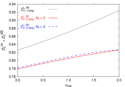
Figure 4: $Z_{V}^{L,RI^{\,\prime}}(a_{{}_{\rm L}}\bar{\mu})=Z_{V}^{L,\overline{MS}}(a_{{}_{\rm L}}\bar{\mu})$ versus $c_{\rm SW}$ ($N_{c}=3$, $\bar{\mu}=1/a_{{}_{\rm L}}$, $\beta_{\circ}=6.0$). Results up to 2 loops are shown for $N_{f}=0$ (solid line) and $N_{f}=2$ (dashed line); one-loop results are plotted with a dotted line.

$$Z_{AV}^{L,RI^{\,\prime}}=1 + \frac{g_{\circ}^{2}}{16\pi^{2}}\,c_{F}\Big{[}-15.796283066(5)-0.247827627(3)\,c_{{\rm SW}}+2.251366176(5)\,c_{{\rm SW}}^{2}\Big{]}$$ (13)

$$+ \frac{g_{\circ}^{4}}{(16\pi^{2})^{2}}\,c_{F}\Big{[}N_{f}\,\Big{(}18.497(3)-1.285(1)\,c_{{\rm SW}}+19.071(3)\,c_{{\rm SW}}^{2}$$

$$\hskip 85.35826pt+1.0333(6)\,c_{{\rm SW}}^{3}-6.7549(6)\,c_{{\rm SW}}^{4}\Big{)}$$

$$\hskip 56.9055pt+c_{F}\,\Big{(}-184.01(1)-389.86(1)\,c_{{\rm SW}}-166.738(6)\,c_{{\rm SW}}^{2}$$

$$\hskip 85.35826pt+7.894(1)\,c_{{\rm SW}}^{3}+4.3201(3)\,c_{{\rm SW}}^{4}\Big{)}$$

$$\hskip 56.9055pt+N_{c}\,\Big{(}-21.62(1)-33.652(5)\,c_{{\rm SW}}+26.636(6)\,c_{{\rm SW}}^{2}$$

$$\hskip 85.35826pt+10.2186(5)\,c_{{\rm SW}}^{3}+1.4893(1)\,c_{{\rm SW}}^{4}\Big{)}\Big{]}$$

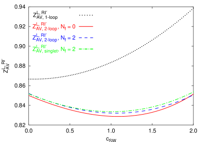
Figure 5: $Z_{AV}^{L,RI^{\,\prime}}(a_{{}_{\rm L}}\bar{\mu})$ versus $c_{\rm SW}$ ($N_{c}=3$, $\bar{\mu}=1/a_{{}_{\rm L}}$, $\beta_{\circ}=6.0$). Results up to 2 loops, for the flavor nonsinglet operator, are shown for $N_{f}=0,\,2$ (solid line, dashed line); 2-loop results for the flavor singlet operator, for $N_{f}=2$, are plotted with a dash-dotted line; one-loop results are plotted with a dotted line.

References

[1]A. Skouroupathis and H. Panagopoulos, Two-loop
renormalization of vector, axial-vector and tensor fermion
bilinears on the lattice, Phys. Rev.D79 (2009)
094508 [arXiv:0811.4264].
[2]A. Skouroupathis and H. Panagopoulos, Two-loop
renormalization of scalar and pseudoscalar fermion
bilinears on the lattice, Phys. Rev.D76 (2007)
094514 [arXiv:0707.2906].
[3] S. Capitani et al., Renormalisation and
off-shell improvement in lattice perturbation
theory,Nucl. Phys.B593 (2001) 183 [hep-lat/0007004].
[4] Y. Aoki, C. Dawson, J. Noaki and A. Soni, Proton
decay matrix elements with domain-wall fermions, Phys. Rev.D75 (2007) 014507 [hep-lat/0607002].
[5] D. Galletly et al., Hadron spectrum, quark
masses and decay constants from light overlap fermions on large
lattices, Phys. Rev.D75 (2007) 073015 [hep-lat/0607024].
[6] M. Della Morte, P. Fritzsch and J. Heitger,
Non-perturbative renormalization of the static axial current
in two-flavour QCD, JHEP0702 (2007) 079 [hep-lat/0611036].
[7] F. Di Renzo, V. Miccio, L. Scorzato and C. Torrero,
High-loop perturbative renormalization constants for Lattice
QCD (I): finite constants for Wilson quark currents,
Eur. Phys. J.C51 (2007) 645 [hep-lat/0611013].
[8] Q. Mason et al., High-precision determination
of the light-quark masses from realistic lattice QCD,
Phys. Rev.D73 (2006) 114501 [hep-ph/0511160].
[9] G. Martinelli et al., A General Method for
Non-Perturbative Renormalization of Lattice Operators,
Nucl. Phys.B445 (1995) 81 [hep-lat/9411010].
[10] J.A. Gracey, Three loop anomalous dimension of
non-singlet quark currents in the RI’ scheme, Nucl. Phys.B662 (2003) 247 [hep-ph/0304113].