Minimax Current Density Coil Design

Abstract

“Coil design” is an inverse problem in which arrangements of wire are designed to generate a prescribed magnetic field when energised with electric current. The design of gradient and shim coils for magnetic resonance imaging (MRI) are important examples of coil design. The magnetic fields that these coils generate are usually required to be both strong and accurate. Other electromagnetic properties of the coils, such as inductance, may be considered in the design process which becomes an optimisation problem. The maximum current density is additionally optimised in this work and the resultant coils are investigated for performance and practicality. Coils with minimax current density were found to exhibit maximally spread wires and may help disperse localized regions of Joule heating. They also produce the highest possible magnetic field strength per unit current for any given surface and wire size. Three different flavours of boundary element method that employ different basis functions (triangular elements with uniform current, cylindrical elements with sinusoidal current and conic section elements with sinusoidal-uniform current) were used with this approach to illustrate its generality.

1 Introduction

In magnetic resonance imaging (MRI) an exquisitely uniform and very intense magnetic field is used to polarize the spin population of a sample so as to maximise the strength of the nuclear magnetic resonance (NMR) signal. A process known as “shimming” is performed at the start of every scan to ensure that this field is as uniform as possible. Shimming involves adjusting the electric current in a set of “shim coils” that each generate a magnetic field of spherical harmonic intensity in the region of interest (ROI). MR images are formed by superimposing magnetic field gradients which causes the frequency of the NMR signal, the Larmor frequency, to vary linearly across the sample. Fourier techniques reconstruct the image from these frequency encoded NMR signals. The linearly varying magnetic fields are generated by “gradient coils”. This paper deals with the design of both gradient and shim coils that dictate the speed, resolution and accuracy of MRI [1].

Gradient and shim coil design is an inverse problem in which arrangements of wire are required to generate a specified magnetic field when energized. Additional considerations are required such as minimal stored energy, so that they may be switched rapidly, or minimal resistive power dissipation, so that their temperature does not increase excessively. As MRI machines get shorter to improve patient comfort [2] so too must the gradient coils [3]. Reducing the length of the gradient coils pushes the wires closer together to maintain magnetic field accuracy. However, gradient and shim coils are constructed from finite sized wire and so there is a minimum wire separation that can be built. In this work the maximum current density was minimized in the coil design process which maximally increases the minimum wire spacing of a coil for fixed coil surface geometry. For a given engineering limit for the minimum spacing between wires this technique can be used to increase the efficiency of the coil (the amount of field per Ampère). It can also be used to reduce the local power dissipation and disperse the hot spots of a coil. The present study demonstrates the design of coils with some increase in inductance or resistance in order to spread wires. Such designs should be judged by appropriate metrics that better encapsulate the coil design problem than those designed to reflect purely the stored energy or power dissipation of the design.

Coil design is also known as magnetic field synthesis and is described by a Fredholm equation of the first kind, which is known to be ill-posed [4]. Early approaches to coil design in MRI cancelled undesired spherical harmonic components of the magnetic field by symmetry and appropriate positioning of loops and arcs of wire (e.g. [5]) or by parameterized surface current densities [6]. The “target field” method [7] circumvented the problem of ill-posedness by employing a Fourier-Bessel expansion of the $\frac{1}{|\mathbf{r}-\mathbf{r}^{\prime}|}$ Green’s function (see §3.11 in Ref. [8]) and defining a continuous target field function for $-\infty<z<\infty$. Since Fourier transforms have unique inverses, it is possible to analytically determine the current density on an infinitely-long cylinder for a limited set of target field functions.

If the target field is defined at a finite set of points, there exists an infinite number of current densities that can produce such a field. With the introduction of the minimum inductance as a constraint [9] the problem becomes regularized and a unique solution exists. This is essentially Tikhonov regularization [10] of the ill-conditioned system of linear equations [11, 12, 13]. This minimum inductance solution was found to be somewhat impractical, so the field was allowed to deviate from its prescribed target values in order to permit a smoother wire pattern. In a related method, a smooth current density was always obtained if it was defined as a weighted sum of a finite number of truncated sinusoidal functions [14, 15, 11, 12, 13]. Parameterizing the current density in this manner allowed more practical, finite-length cylindrical coils with limited spatial frequency to be designed in a method sometimes referred to as the Turner-Carlson method. Minimization of the inductance (the current-normalized stored energy) can be easily substituted by the resistance (the current-normalized power dissipation) while still resulting in a unique solution [16]. For coil designs with asymmetric target field location it is necessary to enforce zero net torque in the presence of an intense background magnetic field [17].

A coil may be defined by its surface current density. The magnitude of that current density defines the wire spacing and the amount of heat generated at positions on the surface. To spread the closest wires or to reduce the local heating, the maximum value of the current density magnitude was incorporated into the coil design problem and its maximum value was minimised. This term is not linear nor quadratic, but only convex with respect to the current density. In contrast to more traditional approaches where only linear systems are solved, we used techniques of convex programming to handle the non-linearities and singularities that arise from the “max” term. We developed an original algorithm to solve this optimisation problem that can be seen as a continuation of two works by Y. Nesterov [18, 19]. It can be shown to converge to the global minimizer of the cost function but details of this algorithm will be presented elsewhere.

The concept of minimum maximum current density (minimax$|j|$) coil design is general and is not limited to any particular coil design method. In this work, three different boundary element methods (BEM) were used to investigate the behaviour of minimax$|j|$ coils. These are the Turner-Carlson [14, 15], triangular [20] and axisymmetric [21, 22] BEMs. The target field was specified at a finite set of discrete points in a region of interest (ROI). The field synthesis problem is defined as minimizing the sum-of-squares field error and is an ill-posed problem. Therefore, a regularizing term must be included to obtain a unique solution.

In a previous attempt to reduce the maximum current density the regularization term was adaptively modified [23]. This method showed a considerable reduction in maximum current density, but it was not known how optimal the solutions were. Other approaches in which regions of the coil were designed manually have been used to control the maximum current density: for example, by predefining the return conductors [24, 25] or by manually introducing a large number of constraints (page 146 of Ref. [21]). The method presented here truly minimizes the maximum current density for coils designed on surfaces of arbitrary shape that generate any physically realizable magnetic field.

2 Methods

2.1 Physical Model

In magnetostatics, Ampère’s Law, $\nabla\times\mathbf{B}(\mathbf{r})=\mu_{0}\mathbf{J}(\mathbf{r})$, relates the magnetic field, $\mathbf{B}(\mathbf{r})$, and the free current density, $\mathbf{J}(\mathbf{r})$. Current density must be conserved, so $\nabla\cdot\mathbf{J}(\mathbf{r})=0$. Employing the magnetic vector potential, $\mathbf{A}(\mathbf{r})$, where $\mathbf{B}(\mathbf{r})=\nabla\times\mathbf{A}(\mathbf{r})$, Ampère’s Law becomes a Poisson equation, $\nabla^{2}\mathbf{A}(\mathbf{r})=\mu_{0}\mathbf{J}(\mathbf{r})$, which has the solution

$$\mathbf{A}(\mathbf{r})=\frac{\mu_{0}}{4\pi}\int\!\!\frac{\mathbf{J}(\mathbf{r}^{\prime})}{|\mathbf{r}-\mathbf{r}^{\prime}|}dV^{\prime}$$ (1)

in the Coulomb gauge ($\nabla\cdot\mathbf{A}(\mathbf{r})=0$). $\mu_{0}$ is the permeability of free-space and has the value $4\pi\times 10^{-7}$ Hm^-1. With some algebra, this leads to the familiar volumetric integral form of the Biot-Savart law [8],

$$\mathbf{B}(\mathbf{r})=\frac{\mu_{0}}{4\pi}\int\mathbf{J}(\mathbf{r}^{\prime})\times\frac{(\mathbf{r}-\mathbf{r}^{\prime})}{|\mathbf{r}-\mathbf{r}^{\prime}|^{3}}dV^{\prime}.$$ (2)

For each directional component of $\mathbf{B}(\mathbf{r})$, (2) is a Fredholm equation of the first kind which is known to be ill-posed. MRI conventionally requires a strong magnetic field for polarization of the nuclear spin states within the sample to be imaged [1]. We consider a system immersed in a background magnetic field, $\mathbf{B}_{0}(\mathbf{r})$, that is highly uniform, unidirectional and very strong, i.e. $\mathbf{B}_{0}(\mathbf{r})=B_{0z}\hat{\mathbf{z}}$, where $\hat{\mathbf{z}}$ is the unit vector parallel to the $z$-axis. The magnitude of the combined magnetic field, $|B_{0z}\hat{\mathbf{z}}+\mathbf{B}(\mathbf{r})|\approx(B_{0z}+B_{z}(\mathbf{r}))$, dictates the local Larmor frequency of the NMR signal and subsequent spatial localization. Therefore we only need to design coils to generate a specific $B_{z}(\mathbf{r})$, justifiably neglecting the two other components, $B_{x}(\mathbf{r})$ and $B_{y}(\mathbf{r})$.

In the context of this paper, “coil design” is the inversion of (2) to design an arrangement of wires that, when energized, form a current density which generates a prescribed magnetic field. The region of space in which the field is prescribed, the ROI, is separate from the region in which the current density exists.

Coil design is rarely as simple as inverting (2) but requires the consideration of other electromagnetic properties. The stored energy, $W$, associated with $\mathbf{J}(\mathbf{r})$ is [8]

$$W=\frac{\mu_{0}}{8\pi}\int_{\Omega_{c}}\!\!\int_{\Omega_{c}}\frac{\mathbf{J}(\mathbf{r})\cdot\mathbf{J}(\mathbf{r}^{\prime})}{|\mathbf{r}-\mathbf{r}^{\prime}|}dVdV^{\prime},$$ (3)

where $\Omega_{c}$ is the region of the coil in which $\mathbf{J}(\mathbf{r})$ is confined to flow. The resistive power dissipation, $P$, is

$$P=\rho_{Cu}\int_{\Omega_{c}}|\mathbf{J}(\mathbf{r})|^{2}dV,$$ (4)

where $\rho_{Cu}$ is the resistivity of the conducting medium which, in this case, is assumed to be copper, $\rho_{Cu}=1.68\times 10^{-10}\Omega$ m.

The coil may be in close proximity to other conducting surfaces defined by the region $\Omega_{e}$. Changing $\mathbf{J}(\mathbf{r})$ in time causes $\mathbf{B}(\mathbf{r})$ to also change, Faraday’s Law, $\nabla\times\mathbf{E}(\mathbf{r})=\frac{\partial\mathbf{B}(\mathbf{r})}{\partial t}$, and $\mathbf{J}(\mathbf{r})=\sigma\mathbf{E}(\mathbf{r})$ show that currents may be induced in other conducting surfaces. These “eddy currents” can cause deleterious effects on MRI. So, a coil designer must consider the effects that the induced eddy currents have on the field in the ROI [26]. For low frequencies ($<$10 kHz) the quasistatic approximation may be used and following the approach of Peeren [27], a Heaviside function response in the coil current was assumed. This leads to a linear relationship between coil currents and eddy currents.

Lorentz forces act on the coil when immersed in a background magnetic field, $\mathbf{B}_{0}$. The net Lorentz force is zero for a divergence-free current density in a uniform $\mathbf{B}_{0}$, but there may exist a consequential net torque, $\boldsymbol{\tau}$,

$$\boldsymbol{\tau}=\int_{\Omega_{c}}\mathbf{r}\times\left[\mathbf{J}(\mathbf{r})\times\mathbf{B}_{0}\right]dV.$$ (5)

Current density was confined to flow on thin surfaces so that a scalar stream-function, $\psi(\mathbf{r})$, can be used to define the vector current density

$$\mathbf{J}(\mathbf{r})=\nabla\times\left[\psi(\mathbf{r})\hat{\mathbf{n}}(\mathbf{r})\right],$$ (6)

where $\hat{\mathbf{n}}(\mathbf{r})$ in the unit vector normal to the surface at $\mathbf{r}$.

2.2 Discrete Formulation

The coil design problem may be solved analytically for some special cases [7] but for other geometries the physical problem must be described by a finite number of parameters in order to apply numerical methods. The type of parameterisation may chosen to best suit the type of coil that is to be designed. $\psi(\mathbf{r})$ can be approximated as a finite weighted sum of $N$ basis functions,

$$\psi(\mathbf{r})\approx\sum_{n}^{N}\psi_{n}\hat{\psi}_{n}(\mathbf{r}),$$ (7)

and so can the current density by combination of (7) with (6),

$$\mathbf{J}(\mathbf{r})\approx\sum_{n}^{N}\psi_{n}\hat{\mathbf{j}}_{n}(\mathbf{r}),$$ (8)

where $\hat{\psi}_{n}(\mathbf{r})$ and $\hat{\mathbf{j}}_{n}(\mathbf{r})$ are the $n$th stream-function and current density basis functions respectively, and $\psi_{n}$ are the weights.

Equation (8) can be incorporated in (2) to (5), so that $B_{z}(\mathbf{r})$, $W$, $P$ and $\boldsymbol{\tau}$ are parameterised as finite summations.

2.3 Matrix Equations

This discrete formulation allows matrix equations for each of the physical properties to be written. A vector of stream-function weights, $\psi$, was defined; $\psi=\left[\psi_{1},\ldots,\psi_{n},\ldots,\psi_{N}\right]^{T}$ (where ^T represents the transpose operation). Each Cartesian component of the current density at a set of points, $\mathbf{r}_{s}$, can be written as matrix equations

$$j_{x}=J_{x}\psi,\quad j_{y}=J_{y}\psi,\quad j_{z}=J_{z}\psi,$$ (9)

where $j_{x}$ is a vector that lists values of the $x$-component of the current density at a set of $S$ points, $j_{x}=\left[J_{x}(\mathbf{r}_{1}),\ldots,J_{x}(\mathbf{r}_{s}),\ldots,J_{x}(\mathbf{r}_{S})\right]^{T}$ and $J_{x}$ in an $S\times N$ matrix. Similar matrix equations can be written for the cylindrical coordinate system to give $j_{\rho}$, $j_{\phi}$ and $j_{z}$.

A $H\times N$ matrix $B$ relates $\psi$ to a vector $b$ of length $H$ containing magnetic field values, where $b=\left[B_{z}(\mathbf{r}_{1}),\ldots,B_{z}(\mathbf{r}_{h}),\ldots,B_{z}(\mathbf{r}_{H})\right]^{T}$;

$$b=B\psi.$$ (10)

Similarly, each component of the torque vector (5) can be written as the inner product of $\psi$ and a vector,

$$\tau_{x}=T_{x}\psi,\quad\tau_{y}=T_{y}\psi,\quad\tau_{z}=T_{z}\psi.$$ (11)

The energy terms (3) and (4) are quadratic with respect to $\psi$,

$$W=\psi^{T}{L_{c}}\psi$$ (12)

$$P=\psi^{T}{R_{c}}\psi$$ (13)

where $L_{c}$ and $R_{c}$ are symmetric, $N\times N$ matrices of the inductance and resistance of the coil surface respectively. In fact, $R_{c}=J_{x}^{T}J_{x}+J_{y}^{T}J_{y}+J_{z}^{T}J_{z}$.

Three types of parameterisation are used in this work. The first assumes that the current-carrying surface is a finite-length cylinder and that $\psi(\mathbf{r})$ is a weighted sum of truncated sinusoidal functions [14, 15]. In the second approach, surfaces are described by flat triangular elements and $\psi(\mathbf{r})$ is a piecewise-linear function [20, 27, 28, 29]. The third approach uses surfaces of revolution about the $z$-axis and is an axisymmetric BEM [21, 22]. The way in which $\psi(\mathbf{r})$ and $\mathbf{J}(\mathbf{r})$ are parameterised in each case are given in the Appendices. For details of how to calculate the matrices, $B$, $T_{x}$, $T_{y}$, $T_{z}$, $L_{c}$, $R_{c}$ for each type of parameterisation, the reader is advised to seek the above references. Other approaches to discretizing the problem are possible, such as using quadrilateral elements, but are not described in the present work.

2.4 Numerical Problem

The vector $\psi$ is a list of the stream-function weights, $\psi_{n}$, which are the free parameters of the coil design problem. The problem including the maximum current density and all other terms can be written generally

$$\min_{\psi\in\Psi}\{U(\psi)=f(\psi)+\alpha e(\psi)+\beta W(\psi)+\gamma P(\psi)+\delta\|j(\psi)\|_{\infty}\}.$$ (14)

It contains terms to control the residual primary field, $f(\psi)$, eddy current field, $e(\psi)$, stored magnetic energy, $W(\psi)$, power dissipation, $P(\psi)$, and maximum current density, $\|j(\psi)\|_{\infty}$, along with their respective, user-definable weighting factors, $\alpha$, $\beta$, $\gamma$ and $\delta$. One, two or three of these parameters are usually set equal to zero to remove them from $U(\psi)$. For example, $\gamma=\delta=0$ will result in an actively shielded, torque-balanced coil with minimal stored energy. Each term in (14) possesses a natural scaling from the physical constants used in their calculation. Choice of $\alpha$, $\beta$, $\gamma$ and $\delta$ values must balance these scalings: for example, $\alpha$, $\beta$, $\gamma$ and $\delta$ are typically in the order 1, $10^{-7}$, $10^{-9}$ and $10^{-10}$ respectively so that they have a magnitude comparable with the $f(\psi)$ term, but are dependent on the specific problem.

The minimization was performed such that $\psi$, belonged to the set of stream-functions, $\Psi$, that exhibit zero net torque (11);

$$\Psi=\{\psi\in\mathbb{R}^{N},\quad T_{x}\psi=0\quad\&\quad T_{y}\psi=0\},$$ (15)

where $T_{x}\psi$ and $T_{y}\psi$ give the $x$- and $y$-components of the torque vector $\tau_{x}$ and $\tau_{y}$, respectively. In this work it was assumed that the background magnetic field was uniform and oriented parallel to $z$, and as such $\tau_{z}=0$. It is also possible to balance the torque of coils immersed in non-uniform background magnetic fields.

The $f$ term in (14) represents the sum-of-squares of the error in the primary magnetic field,

$$f=\frac{1}{2}\|B_{c}\psi-b_{t}\|_{2}^{2},$$

where $\|\cdot\|_{2}$ is the classical $\ell^{2}$-norm, $B_{c}$ is a $H\times N$ matrix relating $\psi$ to the magnetic field values at the $H$ target field points in the ROI (10) and $b_{t}$ is a vector of length $H$ containing the target magnetic field values.

The term $e$ in (14) represents the sum-of-squares of the magnetic field that the eddy currents produce in the ROI. A Heaviside function in coil current was assumed [27] and the stream-function of the instantaneously-induced eddy current density, $\psi_{e}$, is linearly related to $\psi$ by

$$\psi_{e}=-L_{e}^{-1}M_{ec}\psi,$$ (16)

where $L_{e}$ is an $N_{e}\times N_{e}$ ($N_{e}$ is the number of basis functions approximating the current density on the eddy current surface) self-inductance matrix of the conducting surface where eddy currents are induced and $M_{ec}$ is an $N_{e}\times N$ matrix of the mutual inductance between the coil surface and eddy current surface.

The field produced by the eddy current at the target points was desired to be minimal, hence we use the sum-of-squares eddy current field to enforce active magnetic shielding.

$$e=\frac{1}{2}\|B_{e}L_{e}^{-1}M_{ec}\psi\|_{2}^{2},$$ (17)

where $B_{e}$ is a $H\times N_{e}$ matrix relating $\psi_{e}$ to the eddy current magnetic field values at the target points.

The stored magnetic energy, $W$, and power dissipation, $P$, terms in (14) are quadratic with respect to $\psi$ and are given by Equations (12) and (13), respectively.

The maximum current density magnitude in the coil design is written here as the $\ell^{\infty}$-norm of the current density magnitude vector, $j$. $j$ is a list of length $S$ containing the current density magnitude values at each surface point

$$\|j\|_{\infty}=\lim_{p\rightarrow\infty}\left(\sum_{s}(j_{s})^{p}\right)^{1/p}:=\max_{s}\{j_{s}\},$$ (18)

$$j_{s}=|\mathbf{j}_{s}|=\sqrt{j_{sx}^{2}+j_{sy}^{2}+j_{sz}^{2}}.$$ (19)

2.5 Optimization Algorithm

Previous methods solved $\min\{U(\psi)\}$ by partial differentiation of $U(\psi)$, $\frac{\partial U}{\partial\psi}$, and subsequent matrix inversion of the consequential system of linear equations [28, 29]. This cannot be done with (14) since $U(\psi)$ contains a non-differentiable $\ell^{\infty}$ term. To solve (14) we used an accelerated descent algorithm of Nesterov [19] on a dual problem smoothed using ideas of Moreau-Yosida. Full details of the algorithm will be submitted elsewhere. For the purposes of this paper it should be noted that the algorithm requires as inputs the smoothing parameter, $\mu$, for the $\ell^{\infty}$-norm, the number of iterations to perform, $Q$, and an initial guess for the solution, $\psi_{0}$. $\mu$ and $Q$ are related by some inverse relationship that requires more iterations when less smoothing is applied, but will approximate the non-differentiable $\ell^{\infty}$-norm to a greater degree. Convergence was checked by observing the value of the dual cost function as $q\rightarrow Q$.

The optimization algorithm was coded in Matlab (The Mathworks, Natick, MA) and was excecuted on a 64-bit Linux server with Intel (Intel Corporation, Santa Clara, CA) Xeon E5430 quad-core CPUs at 2.66GHz.

2.6 Examples

The impact of designing coils with the minimax$|j|$ was investigated by three examples. These examples are described in the following sections and were chosen to elucidate the behavior of the system when designing realistic coils. In the examples outlined below the convergence rates and calculation times were recorded.

Relevant properties of the coil performance were recorded in all cases. The efficiency, $\eta$, is the intensity of magnetic field that the coil can generate with 1 Amp and is also sometimes referred to as the sensitivity. Inductance, $L$, resistance, $R$, minimum spacing between wires, $w$, maximum field error in the ROI, max($\Delta B_{z}$) and maximum eddy current field in the ROI, max($B_{ez}$), are all recorded. Derived figures-of-merit (FOMs) $\eta^{2}/L$, $\eta^{2}/R$ and $\eta w$ are independent of the number of contours, $N_{c}$, used to convert $\psi$ into wires and are useful for comparing between coils.

2.6.1 Cylindrical X-gradient coils

We initially demonstrate minimax$|j|$ coil design with $\psi(\mathbf{r})$ parameterised by a sum of sinusoidal basis functions [14, 15]. A details the parameterisation of $\psi(\mathbf{r})$ and $\mathbf{J}(\mathbf{r})$. The current-carrying surface for these examples was assumed to be a finite length cylinder 760 mm in diameter. The region of uniformity (ROU) was a 400 mm long, 400 mm diameter cylindrical region positioned concentrically inside the current-carrying surface. The target field in the ROI has a magnitude that varies linearly in the $x$-direction; $B_{z}(\mathbf{r})\propto x$. This simple geometry was used to investigate some of the more fundamental behaviours of coils designed with minimax$|j|$. In all cases $\max{(\Delta B_{z})}$ was kept at $5\pm 0.01$ % and no torque balancing was required because $\mathbf{J}(\mathbf{r})$ is forced to be symmetric by the limited parameterisation. No active shielding was used, so $\alpha=0$.

The length of the coil, $l$, was varied between 700 and 2000 mm to observe its behavior with respect to standard min($W$) and min($P$) coils.

In a second experiment, minimax$|j|$ coils were designed with varying amounts of power minimization to investigate their behavior on the continuum from min($P$) to minimax$|j|$. This was performed with $l$ = 1400 mm, for $N=36$ and 200. For $N=36$, with reference to (20), $M^{\prime}=4$ and $N^{\prime}=8$. For $N=200$, $M^{\prime}=10$ and $N^{\prime}=20$.

2.6.2 Shielded Gradient Coils

Short, cylindrical, actively-shielded gradient coils were designed with minimax$|j|$. The dimensions of a coil presented in Reference [30] was used in this example. The system was modelled with a triangular BEM [20] which approximates $\psi(\mathbf{r})$ as piecewise-linear in each triangle as described in B.

Four different X-gradient coils were designed using different types of minimization, all with max$(\Delta B_{z})=5\pm 0.01\%$ in the ROI and $\alpha$ = 20; min($W$), min($P$), minimax$|j|$ and min($P$ & max$|j|$) which is some combination of min($P$) and minimax$|j|$.

A full set of gradient coils comprises X, Y and Z coils, with Y being a $90^{\circ}$ rotation of the X-gradient. Z-gradient coils ($B_{z}(\mathbf{r})\propto z$) were designed with min($P$), minimax$|j|$and min($P$ and max$|j|$). It is known that for axi-symmetric geometries and target fields (i.e. zonal coils) $\psi(\mathbf{r})$ is $\phi$ invariant. All nodes with identical $\rho_{n}$ and $z_{n}$ were treated together and forced to have the same value of $\psi_{n}$. In some way this is equivalent to the axisymmetric case described in the next example.

2.6.3 Shim Coils

Designing shim coils not only requires the production of magnetic fields that have a different spatial form to gradient coils, but the engineering and electronic requirements are also different. The efficiency, $\eta$, is of primary importance and higher order shims are considerably less efficient than low order shims. Improving $\eta$ for the higher order shim coils would be useful to improve correction of geometric distortion in MR images induced by $\mathbf{B}_{0}$ field error and may provide smaller linewidths for MR spectroscopy via higher order shimming. Due to the often constrained axial and radial space provided for shim coils, wire-spacing can become a problem and limits $\eta$. Coils designed with the minimax$|j|$ were studied to see if they could help improve shim coil performance. X2-Y2 biplanar shim coils ($B_{z}(\mathbf{r})\propto x^{2}-y^{2}$) were designed with 860 mm diameter and 500 mm separation [31]. The ROI is a spherical volume of 380 mm diameter in which max($\Delta B_{z}$) was fixed at $10\pm 0.01$ %. In both cases, the $\phi$ dependence of $\psi(\mathbf{r})$ was spectrally decomposed in terms of 7 sinudoids, i.e. $M^{\prime}=7$, see C.

3 Results

3.1 General Observations

Calculation of the system matrices for both the sum-of-sinusoids and the axisymmetric BEM took on the order of a few seconds. The time required for the triangular BEM system matrix calculations was reduced over previously reported times [29] by coding this part in C. It took less than 10 minutes to calculate all the matrices for a large problem containing 3200 nodes and 6144 triangles. For a medium-sized problem containing 1632 nodes and 3072 triangles the system matrix calculation time was less than 2 minutes.

The optimization algorithm converged in all cases as expected from its deterministic nature. The smoothing parameter, $\mu$, for the $\ell^{\infty}$-norm controls how close the solution to the smoothed problem, $\psi_{\mu}^{\ast}$, is to the true solution, $\psi^{\ast}$. Practically, we make $\mu$ small enough so that no observable difference in the solutions is seen for smaller $\mu$. The time required to find a solution close to $\psi^{\ast}$ varies widely and is dependent on the problem. The number of iterations, $Q$, that the algorithm required to converge is inversely related to $\mu$. For a typical problem tackled in this work, $1\times 10^{-16}\lesssim\mu\lesssim 1\times 10^{-14}$ resulted in indistinguishable solutions which typically required $10,000\lesssim Q\lesssim 200,000$.

3.2 Cylindrical X-gradient coils

The time required to find the solution to a small problem with $\mu=1\times 10^{-15}$, $Q=20,000$ and the number of free variables, $N=36$ was approximately 23 seconds. Figure 1 shows how the FOMs for a) stored energy, b) power dissipation and c) wire spacing varied for min($W$), min($P$) and minimax$|j|$ X-gradient coils as the length of the coil surface varied with max$(\Delta B_{z})=5\pm 0.01\%$. Figure 2 a) shows the values of $\delta$ that were used with varying $\gamma$ to maintain max$(\Delta B_{z})=5\pm 0.01\%$ in the ROU. The variation of the two relevant FOMs with $\gamma$ are shown in Figure 2 b) and c). Figure 3 shows one quadrant of the wire paths for four coils designed with a) min($W$), b) min($P$), c) minimax$|j|$ with N = 200 and d) minimax$|j|$ with N=36. Wire positions are unwrapped from their cylindrical shape onto a flat $z$-$a\phi$ plane. As with all coils presented in this paper, connections must be made during construction from each loop to its neighbour to ensure current flow throughout the coil. The location of these coils are marked for reference on Figure 2 b) and c) where ①, ② and ③ to the coils in Figure 3 b), c) and d) respectively.

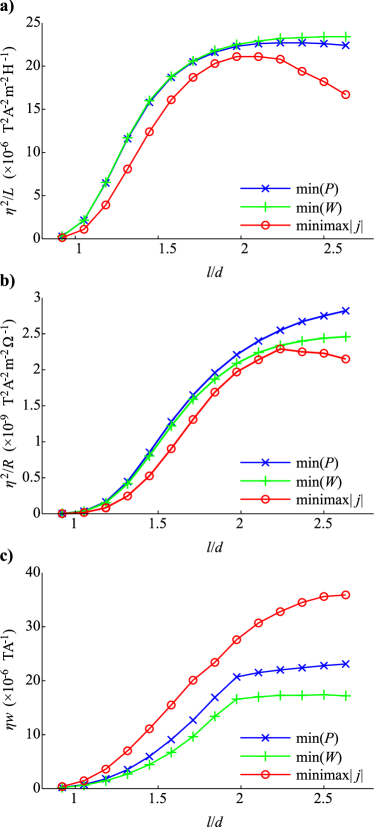
Figure 1: Variation of a) $\eta^{2}/L$, b) $\eta^{2}/R$ and c) $\eta w$ with length-to-diameter ratio, $l/d$ for unshielded X-gradient coils designed with a sum-of-sinusoids parametrised stream function.

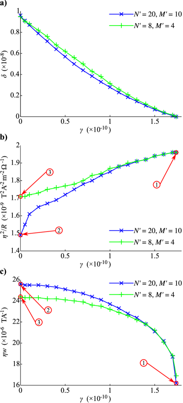
Figure 2: a) $\delta$ values required in combination with varying $\gamma$ in order to maintain field error of $5\pm 0.01$ % with $\beta=0$. b) the resulting $\eta^{2}/R$ and c) $\eta w$ of the coils for 32 and 200 sinusoidal basis functions. Data points labelled ①, ② and ③ correspond to the coils shown in Figure 3 b), c) and d) respectively.

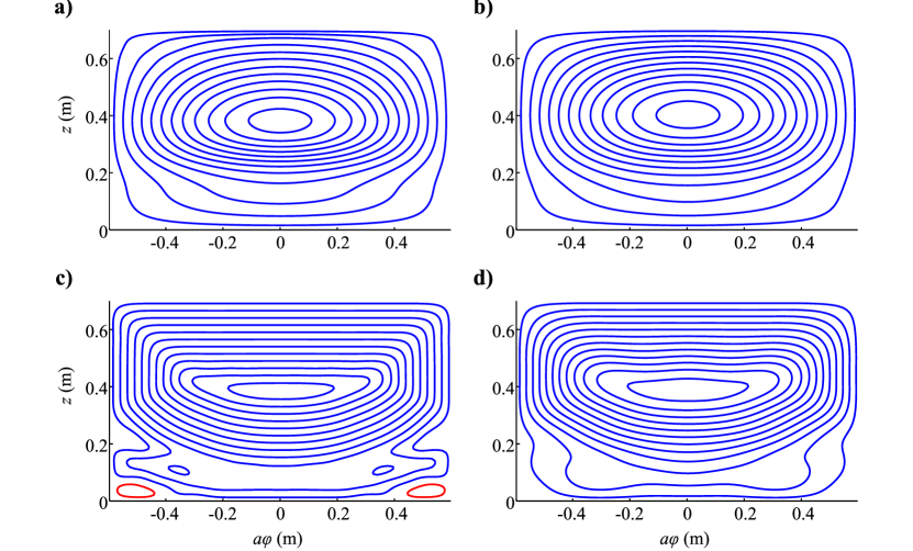
Figure 3: One quadrant each of the wire paths for the sum-of sinusoids, unshielded, X-gradient coils in the cases of a) min($W$), b) min($P$), c) minimax$|j|$ with 200 sinusoids and d) minimax$|j|$ with 32 sinusoids. Red wires indicate reversed current flow with respect to blue and only 12 contours of the stream function are shown for clarity.

3.3 Shielded Gradient Coils

One quadrant of the wire paths for min($W$), min($P$), minimax$|j|$, and min($P$ & max$|j|$) shielded X-gradient coils are shown in Figure 4. The left-hand side show the primary coils and the right-hand side are their active magnetic shields. Their performance characteristics are given in Table 1. Due to the high number of free-parameters, $N=1985$, it took approximately 480 minutes to perform $Q=210,000$ iterations to obtain a well converged solution.

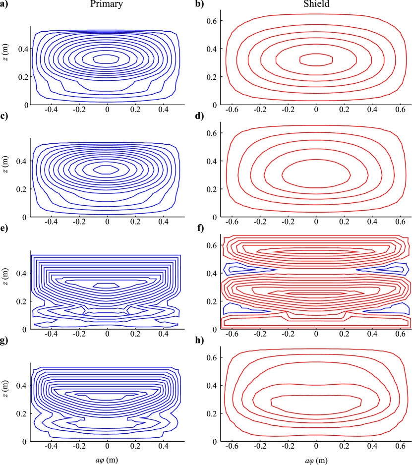
Figure 4: Wire paths for the triangular BEM, actively-shielded, X-gradient coils in the cases of a) and b) min($W$), c) and d) min($P$), e) and f) minimax$|j|$ and g) and h) min($P$ & max$|j|$). The active magnetic screens appear on the right for the primary coils on the left. Red wires indicate reversed current flow with respect to blue and only 12 contours of the stream function are shown for clarity.

Table 1: Properties of the triangular BEM designed, actively-shielded X-gradient coils. Input parameters $\alpha$, $\beta$, $\gamma$, $\delta$ and coil properties including efficiency, $\eta$, maximum field error in the ROU, max($\Delta B_{z}$), maximum eddy current field in the ROU, max($B_{ez}$), inductance, $L$, resistance, $R$, minimum wire spacing, $w$ and figure-of-merit values, $\eta^{2}/L$, $\eta^{2}/R$, $\eta w$.

Property	min($W$)	min($P$)	minimax$|j|$	min($P$ & max$|j|$)
Coil	A	B	C	D
$\alpha$	20	20	20	20
$\beta$	1.54$\times 10^{-7}$	0	0	0
$\gamma$	0	5.5$\times 10^{-9}$	0	$0.5\times 10^{-9}$
$\delta$	0	0	6.3$\times 10^{-9}$	$5.1\times 10^{-9}$
$\eta$, ($\mu$Tm-1A-1)	72.9	71.7	74.0	74.3
max($\Delta B_{z}$) (%)	5.0	5.0	5.0	5.0
max($B_{ez}$) (%)	0.11	0.09	0.16	0.13
$L$ ($\mu$H)	661	654	1621	843
$R$ (m$\Omega$)	132	111	392	158
$w$ (mm)	4.1	6.0	9.3	9.0
$\eta^{2}/L$ (T2m-2A-2H-1)	8.3$\times 10^{-6}$	8.1$\times 10^{-6}$	5.4$\times 10^{-6}$	6.6$\times 10^{-6}$
$\eta^{2}/R$ (T2m-2A${}^{-2}\Omega^{-1}$)	4.0$\times 10^{-8}$	4.6$\times 10^{-8}$	1.4$\times 10^{-8}$	3.5$\times 10^{-8}$
$\eta w$ (TA-1)	3.0$\times 10^{-7}$	4.3$\times 10^{-7}$	6.9$\times 10^{-7}$	6.7$\times 10^{-7}$

The stream-functions of the current densities of the three Z-gradient coils with min($P$), minimax$|j|$, and min($P$ & max$|j|$) are shown in Fig. 5. The FOMs are given in Table 2. The calculation time required to find the optimal solution was dramatically reduced for the Z-gradient coils by reducing the number of free variables. The time required for $Q=80,000$ iterations was 10 minutes for a well converged solution.

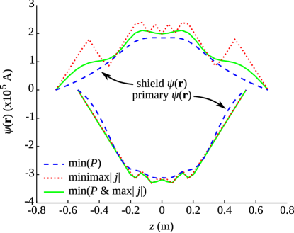
Figure 5: Stream-functions for the actively-shielded, Z-gradient coils designed with min($P$), minimax$|j|$ and min($P$ & max$|j|$). The shield stream functions are greater than zero and the primary stream function are less than zero.

Table 2: Properties of the triangular BEM designed, actively-shielded Z-gradient coils. Input parameters $\alpha$, $\beta$, $\gamma$, $\delta$ and figure-of-merit values, $\eta^{2}/L$, $\eta^{2}/R$, $\eta w$ are given.

Property	min($P$)	minimax$|j|$	min($P$ & max$|j|$)
$\alpha$	20	20	20
$\beta$	0	0	0
$\gamma$	6.1$\times 10^{-9}$	0	5$\times 10^{-10}$
$\delta$	0	7.8$\times 10^{-9}$	7.6$\times 10^{-9}$
$\eta^{2}/L$ (T2m-2A-2H-1)	1.35$\times 10^{-5}$	0.73$\times 10^{-5}$	1.16$\times 10^{-5}$
$\eta^{2}/R$ (T2m-2A${}^{-2}\Omega^{-1}$)	1.44$\times 10^{-8}$	0.60$\times 10^{-8}$	1.05$\times 10^{-8}$
$\eta w$ (TA-1)	8.45$\times 10^{-7}$	11.43$\times 10^{-7}$	11.13$\times 10^{-7}$

3.4 Shim Coils

The wire-paths of one plane of a minimax$|j|$ X2-Y2 biplanar shim coil are shown in Fig. 6 b) next to an equivalent min($P$) coil. Given a 4 mm wire spacing limit for construction, the maximum achievable $\eta$ were 73.8 and 102.0 mTm^-2A^-1 for the min($P$) and minimax$|j|$ coils using $N_{c}=17$ and 20, respectively.

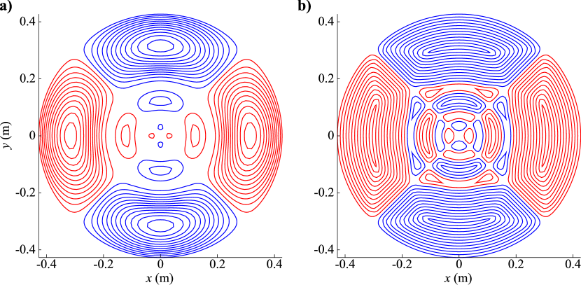
Figure 6: One plane of the wire paths for the axisymmetric BEM designed biplanar X2-Y2 shim coils in the cases of a) min($P$) and b) minimax$|j|$. Red wires indicate reversed current flow with respect to blue.

4 Discussion

This paper reports a method to directly minimize the maximum current density for the magnetic field synthesis or coil design problem. It focuses on the design of gradient and shim coils for MRI applications, but can be considered as a general approach to coil design; it may prove useful outside the realm of gradient and shim coil design. Superconducting magnet design (e.g. see Ref. [32]) is one such application that merits some comment. Although no experiments have yet been performed on magnet design using this minimax optimization, it might be employed to design magnets with reduced peak current density and/or peak magnetic field in the conductors, for example. For practical designs, $\ell^{1}$-norm minimisation of the current density may be incorporated to yield low peak, yet sparse current density designs.

Previous gradient coil design methods have very effectively minimized the stored energy [9] and power dissipation [16] subject to the production of magnetic fields of a prescribed accuracy. Other approaches that lower the maximum current density have been presented [21, 23, 31], but none can be shown to be optimal in terms of minimax current density. We used the adaptive regularisation technique [23] to design shielded X-gradient coils shown in Fig. 4 and found that it could achieve a minimum wire spacing of 8.7 mm. The minimax$|j|$ algorithm achieved 9.3 mm wire spacing indicating that adaptive regularisation works well, but cannot maximally spread the wires. The reason for the difficulty in achieving truly minimax current density coils is that such a term is non-differentiable with respect to the solution variables. It is surely possible to insert such a non-differentiable term into a stochastic optimization technique such as a genetic algorithm [33] or simulated annealing [34], but it is expected that such methods would require very long computing times and converge to a solution that is not necessary the global one. Here, the maximum operation is expressed as the infinity norm (also known as the uniform or Chebychev norm), $\|\cdot\|_{\infty}$, smoothed and converted to its norm-dual, the $\ell^{1}$-norm.

The time required for this algorithm to converge varies widely on the size of the $(S\times N)$ current density matrices, $J_{x}$, $J_{y}$ and $J_{z}$. For the Turner-Carlson approach [7, 9, 14, 15] with $N=32$ and $S=441$ convergence was obtained in 23 seconds. However, for $N=1985$ and $S=4096$ with the triangular BEM it took 480 minutes. It should be noted that for $\delta=0$, the solution is obtained in less than a second as just one matrix inversion is needed [28, 29]. This illustrates the need to take into account any symmetry that might be present in the system to lower the number of free variables and speed up the calculation. For a defined maximum field error, the design process needs to be repeated in order to obtain the ideal trade-off parameter, $\delta$. It is hoped that the amount of user input and computational burden can be reduced by describing the problem as a constrained one in which maximum field error is a user-definable constraint.

The length of an unshielded X gradient coil was varied such that the length-to-diameter ratio, $l/d$, ranged from 0.92 to 2.63. The performance of the coils designed with min($W$), min($P$) and minimax$|j|$ were evaluated and Figure 1 shows the dependencies of $\eta^{2}/L$, $\eta^{2}/R$ and $\eta w$ on coil length. $\eta^{2}/L$ characterises the power requirements of the driving amplifier and $\eta^{2}/R$ characterises the total amount of heat generated by the coil where higher values indicate better performance in both cases. $\eta w$ on the other hand characterises the maximum field strength that can be obtained irrespective of inductance or resistance for a given minimum wire spacing. Several interesting behaviours are apparent from studying the data in Figure 1. First, when designing a coil with min($W$) it will have the highest $\eta^{2}/L$ value. Likewise, a min($P$) coil will have the highest $\eta^{2}/R$ value and minimax$|j|$ coils will have the highest $\eta w$. This is to be expected. min($W$) and min($P$) designed coils have very similar $\eta^{2}/L$ values and slightly different $\eta^{2}/R$ values, with the minimax$|j|$ coils possessing lower values of these two FOMs. In fact, for very long coils ($l/d\gtrsim 2.2$), the value of $\eta^{2}/L$ and $\eta^{2}/R$ actually decreases for the minimax$|j|$ coils. However, the minimax$|j|$ coils possess a $\eta w$ value that is considerably larger than that of the min($W$) and min($P$) designed coils. Figure 1 c) shows that for min($W$) and min($P$) coils with $l/d\gtrsim 2$ the value of $\eta w$ becomes flat. This happens when the region of max$|j|$ occurs approximately at the end of the ROI and not at the end of the coil. This indicates that the length of the coil surface is no longer restricting the maximum achievable field strength when $l/d\gtrsim 2$. $\eta w$ appears to be tending to a particular value for long minimax$|j|$ coils that is approximately 1.5 to 2 times larger than the other coils. Unlike a previous approach [23], minimax current density coils are dramatically different from their Tikhonov regularized counterparts even for long cylindrical coils.

It is known that a unique solution is found when ill-posed problems are solved with Tikhonov regularisation, which is the case for min($W$) and min($P$). It is not known if a unique solution results from including the minimax$|j|$ term in the functional. It is suspected by the authors that there is no unique solution, but more theoretical analysis is required to establish this. Figure 2 shows the behavior when $\beta=0$ and both $\gamma$ and $\delta$ are finite, i.e. as min($P$) is traded for minimax$|j|$ in the optimisation. The $\delta$ value required to maintain a constant field error is inversely related to $\gamma$, as expected. $\gamma$ and $\delta$ values are similar for $N=32$ and 200 sinusoidal basis functions. Figure 2 b) shows the variation of the power FOM, $\eta^{2}/R$, as this trade-off happens. It is evident from these data that by adding a small amount of $\gamma$ to the minimax$|j|$ coil, a sharp increase in $\eta^{2}/R$ can be effected at the expense of very little decrease in $\eta w$. When $N=32$ more smoothness is enforced by the basis functions and $P$ is limited. Hence $\eta^{2}/R$ is lower when more basis functions are used, indicated by ② and ③ on Figure 2 b), but $\eta w$ is also limited. This difference is also evident in Figures 3 c) and d). Conversely, Figure 2 c) shows that by adding a small amount of $\delta$ to the min($P$) coil, a large increase in $\eta w$ can be achieved with only a small change in the power dissipation of the coil. It is not surprising to observe that both min($P$) coils with $N=32$ and 200 are essentially the same since min($P$) coils favour low spatial frequencies in $\psi(\mathbf{r})$. It is clearly possible to choose any solution on the continuum from min($P$) to minimax$|j|$. Although not presented in this paper, it is also possible to trade min($W$) with minimax$|j|$ along a similar continuum.

From Figure 3 it can be seen that the min($W$) coil possesses an area with the highest current density at the ends of the primary with the wires of the power minimized coil being more spread, as expected [16]. $\psi(\mathbf{r})$ conforms to the usual $\cos{\phi}$ dependence for the min($W$) and min($P$) coils despite no such constraint. However, this leads to regions of higher current density at $\phi=0$ which is optimally dispersed in the minimax$|j|$ coils. Deviation from the $\cos{\phi}$ behavior at the ends of the coils means that spherical harmonic fields of higher degree will be introduced in the ROI. These high degrees are then cancelled by $\psi(\mathbf{r})$ variations closer to the ROI.

Incorporating active magnetic shielding [26] into the functional is a simple matter since it can be written in a similar form as the target field term. Actively-shielded X-gradient coils were designed using the same geometry as appears in Reference [30]. Figure 4 shows one quadrant each of the primary and shield wire paths of the min($W$), min($P$), minimax$|j|$ and min($P$ & max$|j|$). It is interesting to note that the shield coil for the purely minimax$|j|$ coil has unnecessary current density with many reversed turns, Figure 4 f). This results from the fact that there is no penalty for extra current density when $\beta$ and $\gamma$ are zero. By incorporating a small amount of $\gamma$, this impractical design is very effectively converted into a highly practical design with smooth wire paths, low resistance and very well spread wires, Figure 4 h). It would also be simple to have different $\gamma$ and $\delta$ values for primary and shield coils. The wire paths in Figure 4 e) show the tendency of minimax$|j|$ in an extreme case where right-angular corners appear in the design.

Similar, but less pronounced effects were observed from the results of the Z-gradient coil of identical geometry. Figure 5 shows the stream functions along the $z$-direction for the coils designed with max$(\Delta B_{z})=5\pm 0.01$ %. The magnitude of the current density (in this case the steepness of the slope of the stream-function) is almost the same in all parts of the coil. This again leads to unnecessarily large amounts of current density on the shield coil, which is easily removed by the addition of a small value of $\gamma$. The combined min($P$ & max$|j|$) Z-gradient coil exhibits large wire spacing and marginally increased resistance when compared to the min($P$) coil. The problems associated with high current densities are less severe when compared to those of X-gradient coils, but this approach may be more useful for zonal shim coils of higher order.

In a final example, an axisymmetric BEM was used to design biplanar X2-Y2 shim coils. Rotational symmetry of the system about the $z$-axis is assumed. $\psi(\mathbf{r})$ is spectrally decomposed in $\phi$ and spatially in $\rho$ and $z$. Qualitatively, it can be seen from Figure 6 that the minimax$|j|$ coil used all the space provided, whereas the min($P$) coil forced wires to be very smooth. For a fixed max$(\Delta B_{z})=10\pm 0.01$ % and $w\geq 4$ mm, $\eta$ is 38% higher for the minimax$|j|$ coil. The construction of such coils may be made slightly more complex by the additional loops in the design. Again, a combined min($P$ & max$|j|$) coil might provide a good balance between simplicity and efficiency.

5 Conclusion

It has been shown that the magnetostatic field synthesis problem can be solved for coils with minimax current density. The problem was solved in the present study with three different boundary element methods to illustrate the generality of the approach. It can therefore be used to synthesize any physically realistic magnetic field with currents flowing on arbitrary surfaces. Alternatively, the time needed to solve the problem can be dramatically reduced by assuming some degree of symmetry. Coils with minimax current density possessed increased resistance and inductance for the same field error and in some cases had high current densities in regions known to naturally require only low current density. More practical coils were obtained with a mixture of power and maximum current density minimization. Such coils are characterized by low inductance and resistance, but also a large spacing between all the wires of the coil. This spreading of wires may be used to increase the efficiency of the coil by permitting extra turns to be added, reduce turn-to-turn eddy current effects, reduce localized heating in the coil, and design coils that are easier to manufacture and/or are extremely short. Moreover, it allows a coil designer to explore a new range of optimal solutions to the field synthesis problem. The resultant coils must be judged by figures-of-merit appropriate to the desired characteristics of the coil, since field accuracy, gradient efficiency, stored energy, power dissipation and maximum current density may all be traded for each other.

6 Acknowledgements

This work was performed for MedTeQ, a Queensland smart state funded research centre. The authors wish to thank Prof. Richard Bowtell for his invaluable assistance with preliminary work on the coil design methods used in this study.

Appendix A Sum-of-Sinusoids

In this appendix we present for completeness the formulation for calculating the matrices in Equations (8) to (13) necessary for implementing the minimax current density algorithm with sinusoidal stream-function basis functions. In this case, the coil surface is assumed to be a finite-length, $l$, cylinder of radius $a$ with its axis of symmetry oriented in the $z$ direction. The stream-function of the current density, $\psi(\mathbf{r})$, is spectrally decomposed and assumed to be a finite weighted sum of truncated sinusoidal functions in $z$ and $\phi$;

$$\psi(\phi,z)=\sum_{m^{\prime}=1}^{M^{\prime}}\sum_{n^{\prime}=1}^{N^{\prime}}\lambda_{m^{\prime}n^{\prime}}\hat{\psi}_{m^{\prime}n^{\prime}}(\phi,z)$$ (20)

where

$$\hat{\psi}_{m^{\prime}n^{\prime}}(\phi,z)=\cases{\sin{\left(\frac{2\pi n^{\prime}}{l}z\right)}\cos{\left((2m^{\prime}-1)\phi\right)}&if $|z|\leq\frac{l}{2}$\\ 0&if $|z|>\frac{l}{2}$\\ }.$$ (21)

The prime indicates the difference between $n$ used in the main algorithm and the order, $n^{\prime}$, and degree, $m^{\prime}$, of the sinusoid. Equation (7) is obtained by a reordering of the weights $\lambda_{m^{\prime}n^{\prime}}$ as $\psi_{n}$. It restricts the magnetic field to be antisymmetric in the $x$-direction and symmetric in the $z$-direction. Extra basis functions that are symmetric in $x$ and antisymmetric in $z$ can be included in order to remove the inherent field symmetry enforcement [11, 12, 13], but this is not required in the present study since we are designing an X-gradient coil and know that $\psi(\mathbf{r})=0$ at $|\phi|=\frac{\pi}{2}$. Due to this enforced symmetry it is known that the net torque experienced by the coil is zero.

The current density on the coil surface has $J_{\phi}$- and $J_{z}$-components that are

$$J_{\phi}(\phi,z)=\frac{\partial\psi}{\partial z}=\sum_{m^{\prime}}^{M^{\prime}}\sum_{n^{\prime}}^{N^{\prime}}\lambda_{m^{\prime}n^{\prime}}\frac{2\pi n^{\prime}}{l}\cos{\left(\frac{2\pi n^{\prime}}{l}z\right)}\cos{\left((2m^{\prime}-1)\phi\right)}$$ (22)

$$J_{z}(\phi,z)=\frac{-\partial\psi}{a\partial\phi}=\sum_{m^{\prime}}^{M^{\prime}}\sum_{n^{\prime}}^{N^{\prime}}\lambda_{m^{\prime}n^{\prime}}\frac{m^{\prime}}{a}\sin{\left(\frac{2\pi n^{\prime}}{l}z\right)}\sin{\left((2m^{\prime}-1)\phi\right)}$$ (23)

and are equivalent to (8) and (9).

Appendix B Triangular Boundary Elements

A surface can be meshed as a series of $I$ triangular elements with $N$ nodes at the corners of the triangles [20]. In this case, $\psi(\mathbf{r})$ is piecewise-linear in each triangle and the stream-function values at the node positions, $\psi_{n}$, define the whole stream-function;

$$\psi(\mathbf{r})=\sum_{n=1}^{N}\psi_{n}\sum_{i=1}^{I}\hat{\psi}_{ni}(\mathbf{r})$$ (24)

where

$$\hat{\psi}_{ni}(\mathbf{r})=1-\frac{(\mathbf{r}-\mathbf{r}_{n})\cdot\mathbf{d}_{ni}}{|\mathbf{d}_{ni}|}$$ (25)

if $\mathbf{r}$ is a point in triangle $i$ and $n$ is a node of that triangle. $\hat{\psi}_{ni}(\mathbf{r})=0$ otherwise. It is possible to use higher order shape functions over the triangle so long as they form a divergence-free basis [35].

The current density on the surface is found from (24), (25) and (6) yielding (8) and

$$\hat{\mathbf{j}}_{n}(\mathbf{r})=\sum_{i}^{I}\mathbf{v}_{ni}(\mathbf{r})=\sum_{i}^{I}\frac{\mathbf{e}_{ni}}{2A_{i}}$$ (26)

if $\mathbf{r}$ is a point in triangle $i$ and $n$ is a node of that triangle. $\mathbf{v}_{ni}(\mathbf{r})=0$ otherwise. $A_{i}$ is the area of the triangle $i$ and $\mathbf{e}_{ni}$ is the vector that describes the edge of the $i$th triangle opposite the $n$th node. This demonstrates that the current density is uniform over each element of the mesh and so that there needs to be one current density sample for each $I$ triangles in order to fully characterise it. Therefore $s$ becomes $i$ and $S$ is equal to the number of triangles, $I$.

Appendix C Axi-symmetric Boundary Elements

The axisymmetric BEM is used for coil supports that can be described by surfaces of revolution about the $z$-axis. Each “node”, $n^{\prime}$, of this surface is in fact a circle in the $xy$-plane and defined by its radius, $\rho_{n^{\prime}}$ and axial position $z_{n^{\prime}}$. There may be a conical element, $i$, either side of each node, labelled $+$ and $-$. A local coordinate, $\zeta(\rho,z)$, is defined for each element that is 0 at one end and 1 at the other. Positions on these two conical surfaces are

$$\begin{array}[]{c}\mathbf{r}_{n}^{+}(\zeta,\phi)=\left(\!\!\!\begin{array}[]{c}\rho_{n}\\ \phi\\ z_{n}\\ \end{array}\!\!\!\right)+\zeta\left(\!\!\!\begin{array}[]{c}\rho_{n+1}-\rho_{n}\\ 0\\ z_{n+1}-z_{n}\\ \end{array}\!\!\!\right)\\ \\ \mathbf{r}_{n}^{-}(\zeta,\phi)=\left(\!\!\!\begin{array}[]{c}\rho_{n-1}\\ \phi\\ z_{n-1}\\ \end{array}\!\!\!\right)+\zeta\left(\!\!\!\begin{array}[]{c}\rho_{n}-\rho_{n-1}\\ 0\\ z_{n}-z_{n-1}\\ \end{array}\!\!\!\right)\\ \\ \end{array}$$ (27)

The surface and therefore $\psi(\mathbf{r})$ are parameterised in $\rho$ and $z$. $\psi(\mathbf{r})$ is decomposed spectrally parameterised in the $\phi$-direction as a sum of sinusoids. In section §2.6.3 an X2-Y2 shim coil is designed that has a target magnetic field with 2-fold rotational symmetry about $z$. Therefore, $\psi(\mathbf{r})$ is restricted in the $\phi$-direction to take the form $\cos{(2(2m^{\prime}-1)\phi)}$. As described in A, the basis function weights, $\lambda_{m^{\prime}n^{\prime}}$ can be reordered to comply with the vector arrangement, $\psi$, in the main algorithm.

$$\psi(\zeta,\phi)=\sum_{m^{\prime}}^{M^{\prime}}\sum_{n^{\prime}}^{N^{\prime}}\lambda_{m^{\prime}n^{\prime}}\sum_{i}^{I}\hat{\psi}_{m^{\prime}n^{\prime}i}(\zeta)\cos{(2(2m^{\prime}-1)\phi)}$$ (28)

where

$$\hat{\psi}_{m^{\prime}n^{\prime}i}(\zeta)=(1-\zeta)$$ (29)

if $i$ is on the positive side of $n^{\prime}$, for $0\leq\zeta\leq 1$,

$$\hat{\psi}_{m^{\prime}n^{\prime}i}(\zeta)=\zeta$$ (30)

if $i$ is on the negative side of $n^{\prime}$, for $0\leq\zeta\leq 1$ and $\hat{\psi}_{m^{\prime}n^{\prime}i}(\zeta)=0$ otherwise.

The stream-function (6) is applied to obtain, after considerable amounts of algebra, the discretised current density

$$\mathbf{J}(\mathbf{r})=\sum_{m^{\prime}}^{M^{\prime}}\sum_{n^{\prime}}^{N^{\prime}}\lambda_{m^{\prime}n^{\prime}}\sum_{i}^{I}\mathbf{v}_{m^{\prime}n^{\prime}i}(\mathbf{r})$$ (31)

where

$$\mathbf{v}_{m^{\prime}n^{\prime}i}(\mathbf{r}) =\left[\frac{\cos(2(2m^{\prime}-1)\phi)\sin\phi}{\sqrt{(\rho_{n+1}-\rho_{n})^{2}+(z_{n+1}-z_{n})^{2}}}\right.$$ (32)

$$\left.+\frac{m^{\prime}(1-\zeta)(\rho_{n+1}-\rho_{n})\sin(2(2m^{\prime}-1)\phi)\cos\phi}{\sqrt{(\rho_{n+1}-\rho_{n})^{2}+(z_{n+1}-z_{n})^{2}}(\rho_{n}+\zeta(\rho_{n+1}-\rho_{n}))}\right]\mathbf{\hat{x}}$$

$$+\left[\frac{-\cos(2(2m^{\prime}-1)\phi)\cos\phi}{\sqrt{(\rho_{n+1}-\rho_{n})^{2}+(z_{n+1}-z_{n})^{2}}}\right.$$

$$\left.+\frac{m^{\prime}(1-\zeta)(\rho_{n+1}-\rho_{n})\sin(2(2m^{\prime}-1)\phi)\sin\phi}{\sqrt{(\rho_{n+1}-\rho_{n})^{2}+(z_{n+1}-z_{n})^{2}}(\rho_{n}+\zeta(\rho_{n+1}-\rho_{n}))}\right]\mathbf{\hat{y}}$$

$$+\left[\frac{m^{\prime}(1-\zeta)(z_{n+1}-z_{n})\sin(2(2m^{\prime}-1)\phi)}{\sqrt{(\rho_{n+1}-\rho_{n})^{2}+(z_{n+1}-z_{n})^{2}}(\rho_{n}+\zeta(\rho_{n+1}-\rho_{n}))}\right]\mathbf{\hat{z}}$$

if $i$ is on the positive side of $n^{\prime}$, for $0\leq\zeta\leq 1$ and $0\leq\phi<2\pi$,

$$\mathbf{v}_{m^{\prime}n^{\prime}i}(\mathbf{r}) =\left[\frac{-\cos(2(2m^{\prime}-1)\phi)\sin\phi}{\sqrt{(\rho_{n}-\rho_{n-1})^{2}+(z_{n}-z_{n-1})^{2}}}\right.$$ (33)

$$\left.+\frac{m^{\prime}\zeta(\rho_{n}-\rho_{n-1})\sin(2(2m^{\prime}-1)\phi)\cos\phi}{\sqrt{(\rho_{n}-\rho_{n-1})^{2}+(z_{n}-z_{n-1})^{2}}(\rho_{n-1}+\zeta(\rho_{n}-\rho_{n-1}))}\right]\mathbf{\hat{x}}$$

$$+\left[\frac{\cos(2(2m^{\prime}-1)\phi)\cos\phi}{\sqrt{(\rho_{n}-\rho_{n-1})^{2}+(z_{n}-z_{n-1})^{2}}}\right.$$

$$\left.+\frac{m^{\prime}\zeta(\rho_{n}-\rho_{n-1})\sin(2(2m^{\prime}-1)\phi)\sin\phi}{\sqrt{(\rho_{n}-\rho_{n-1})^{2}+(z_{n}-z_{n-1})^{2}}(\rho_{n-1}+\zeta(\rho_{n}-\rho_{n-1}))}\right]\mathbf{\hat{y}}$$

$$+\left[\frac{m^{\prime}\zeta(z_{n}-z_{n-1})\sin(2(2m^{\prime}-1)\phi)}{\sqrt{(\rho_{n}-\rho_{n-1})^{2}+(z_{n}-z_{n-1})^{2}}(\rho_{n-1}+\zeta(\rho_{n}-\rho_{n-1}))}\right]\mathbf{\hat{z}}$$

if $i$ is on the negative side of $n^{\prime}$, for $0\leq\zeta\leq 1$ and $0\leq\phi<2\pi$ and $\mathbf{v}_{m^{\prime}n^{\prime}i}(\mathbf{r})=0$ otherwise.

References

References

- [1] J.-M. Jin. Electromagnetic Analysis and Design in Magnetic Resonance Imaging. CRC Press LLC, (1998).
- [2] S. Crozier and D. M. Doddrell. Compact MRI Magnet Design by Stochastic Optimization. Journal of Magnetic Resonance, 127(2), 233 – 237, (1997).
- [3] S. Shvartsman, M. Morich, G. Demeester, and Z. Zhai. Ultrashort Shielded Gradient Coil Design with 3D Geometry. Concepts in Magnetic Resonance Part B: Magnetic Resonance Engineering, 26B(1), 1–15, (2005).
- [4] K. Adamiak. On Fredholm Integral Equations of the First Kind Occurring in Synthesis of Electromagnetic Fields. International Journal for Numerical Methods in Engineering, 17(8), 1187–1200, (1981).
- [5] F. Roméo and D. I. Hoult. Magnet Field Profiling: Analysis and Correcting Coil Design. Magnetic Resonance in Medicine, 1(1), 44–65, (1984).
- [6] M. J. E. Golay. Field Homogenizing Coils For Nuclear Spin Resonance Instrumentation. Review of Scientific Instruments, 29(4), 313–315, (1958).
- [7] R. Turner. A Target Field Approach To Optimal Coil Design. Journal of Physics D: Applied Physics, 19(8), L147–L151, (1986).
- [8] J. D. Jackson. Classical Electrodynamics, 3rd Edition. John Wiley and Sons, Ltd., (1998).
- [9] R. Turner. Minimum Inductance Coils. Journal of Physics E: Scientific Instruments, 21(10), 948–952, (1988).
- [10] A. N. Tikhonov and V. Y. Arsenin. Solutions of ill-posed problems. John Wiley & Sons, New York, (1977).
- [11] L. K. Forbes and S. Crozier. A Novel Target-Field Method For Finite-Length Magnetic Resonance Shim Coils: I. Zonal Shims. Journal of Physics D: Applied Physics, 34(24), 3447–3455, (2001).
- [12] L. K. Forbes and S. Crozier. A Novel Target-Field Method For Finite-Length Magnetic Resonance Shim Coils: II. Tesseral Shims. Journal of Physics D: Applied Physics, 35(9), 839–849, (2002).
- [13] L. K. Forbes and S. Crozier. A Novel Target-Field Method For Magnetic Resonance Shim Coils: III. Shielded Zonal And Tesseral Coils. Journal of Physics D: Applied Physics, 36(2), 68–80, (2003).
- [14] Z. J. J. Stekly. Continuous, Transverse Gradient Coils With High Gradient Uniformity. Proceedings of the Society for Magnetic Resonance in Medicine, 4, 1121, (1985).
- [15] J. W. Carlson, K. A. Derby, K. C. Hawryszko, and M. Weideman. Design And Evaluation Of Shielded Gradient Coils. Magnetic Resonance in Medicine, 26(2), 191–206, (1992).
- [16] R. Turner. Gradient Coil Design: A Review Of Methods. Magnetic Resonance Imaging, 11(7), 903–920, (1993).
- [17] A. M. Abduljalil, A. H. Aletras, and P. M. L. Robitaille. Torque Free Asymmetric Gradient Coils For Echo-Planar Imaging. Magnetic Resonance In Medicine, 31(4), 450–453, (1994). MF.
- [18] Y. Nesterov. Smooth minimization of non-smooth functions. Mathematical Programming, 103(1), 127–152, (2005).
- [19] Y. Nesterov. Gradient methods for minimizing composite objective function. CORE Discussion Papers 2007076, Universit catholique de Louvain, Center for Operations Research and Econometrics (CORE), (2007).
- [20] S. Pissanetzky. Minimum Energy MRI Gradient Coils of General Geometry. Measurement Science and Technology, 3(7), 667–673, (1992).
- [21] G. N. Peeren. Stream Function Approach For Determining Optimal Surface Currents. PhD thesis, Technische Universiteit Eindhoven, (2003).
- [22] M. Poole and R. Bowtell. Azimuthally Symmetric IBEM Gradient and Shim Coil Design. Proceedings of the International Society for Magnetic Resonance in Medicine, 16, 345, (2008).
- [23] M. Poole, H. Sanchez Lopez, and S. Crozier. Adaptively Regularised Gradient Coils or Reduced Local Heating. Concepts in Magnetic Resonance Part B: Magnetic Resonance Engineering, 33B(4), 220–227, (2008).
- [24] R. A. Compton. Gradient-Coil Apparatus for a Magnetic Resonance System, US Patent, 4,456,881, (1984).
- [25] P. Konzbul and K. Švéda. Shim Coils for NMR and MRI Solenoid Magnets. Measurement Science and Technology, 6(8), 1116–1123, (1995).
- [26] P. Mansfield and B. Chapman. Active Magnetic Screening of Coils for Static and Time-Dependent Magnetic Field Generation in NMR Imaging. Journal of Physics E: Scientific Instruments, 19(7), 540–545, (1986).
- [27] G. N. Peeren. Stream Function Approach For Determining Optimal Surface Currents. Journal of Computational Physics, 191(1), 305–321, (2003).
- [28] R. A. Lemdiasov and R. Ludwig. A Stream Function Method For Gradient Coil Design. Concepts in Magnetic Resonance Part B: Magnetic Resonance Engineering, 26B(1), 67–80, (2005).
- [29] M. Poole and R. Bowtell. Novel Gradient Coils Designed Using a Boundary Element Method. Concepts in Magnetic Resonance Part B: Magnetic Resonance Engineering, 31B, 162–175, (2007).
- [30] S. Shvartsman and M. C. Steckner. Discrete Design Method of Transverse Gradient Coils for MRI. Concepts in Magnetic Resonance Part B: Magnetic Resonance Engineering, 31B(2), 95–115, (2007).
- [31] M. Zhu, L. Xia, F. Liu, and S. Crozier. Deformation-Space Method for the Design of Biplanar Transverse Gradient Coils in Open MRI Systems. Magnetics, IEEE Transactions on, 44(8), 2035–2041, (2008).
- [32] H. Xu, S. Conolly, G. Scott, and A. Macovski. Homogeneous magnet design using linear programming. Magnetics, IEEE Transactions on, 36(2), 476–483, (2000).
- [33] B. J. Fisher, N. Dillon, T. A. Carpenter, and L. D. Hall. Design By Genetic Algorithm Of A Z-Gradient Set For Magnetic-Resonance-Imaging Of The Human Brain. Measurement Science and Technology, 6(7), 904–909, (1995).
- [34] S. Crozier and M. Doddrell. Gradient Coil Design by Simulated Annealing. Journal of Magnetic Resonance Series A, 103, 354–357, (1993).
- [35] C. Cobos Sánchez, L. Marin, R. W. Bowtell, H. Power, P. Glover, A. A. Becker, and I. A. Jones. Application of Higher-Order Boundary Element Method to Gradient Coil Design. Proceedings of the British Chapter of the International Society for Magnetic Resonance in Medicine, 12, P23, (2006).