New Exact Solutions of a Generalized Shallow Water Wave Equation

Abstract

In this work an extended elliptic function method is proposed and applied to the generalized shallow water wave equation. We systematically investigate to classify new exact travelling wave solutions expressible in terms of quasi-periodic elliptic integral function and doubly-periodic Jacobian elliptic functions. The derived new solutions include rational, periodic, singular and solitary wave solutions. An interesting comparison with the canonical procedure is provided. In some cases the obtained elliptic solution has singularity at certain region in the whole space. For such solutions we have computed the effective region where the obtained solution is free from such a singularity.

Keywords: Shallow Water Wave Equation, Integrable Systems, Travelling Waves,
                  Jacobian Elliptic Function, Rational Solution, Singular Solution.

PACS number(s): 02.30.Jr, 02.30.Ik, 05.45.-a

1 Introduction

Seeking analytical as well as numerical solutions of nonlinear systems has continued to attract attention through the last few decades [1, 2, 3, 4, 5]. Mathematically, nonlinear equations do not normally have solutions which would superpose making the systems they represent rather complicated and difficult to analyze [6, 7]. On the other hand, an extensive study of a number of nonlinear systems has revealed that there do exist solutions which are not only interesting in their own right but have a wide range of applicability [8, 9]. To generate exact solutions and to understand their properties several important techniques have been developed such as the inverse scattering approach [10], Lax pair formulation [11], Backlund transformations [12] and Hirota’s bilinear method [13, 14]. Nonlinear equations have also been shown to arise from a boundary value problem [15] possessing hierarchy of conservation laws [16].

An important class of solutions of nonlinear evolution equations is concerned with those of the travelling waves that reduce the guiding partial differential equation of two variables namely, $x$ and $t$ to an ordinary differential equation of one independent variable $z=x-\textrm{c}t$ where $\textrm{c}(\in\mathbb{R}-\{0\})$ is a parameter signifying the speed with which the wave travels either to the right or left. A number of methods has been employed in the literature to obtain the travelling wave solutions of various types. Of these the tanh-method stands out as one of the very effective tools for solving certain classes of nonlinear evolution and wave equation [17]. Others include the variational iteration method for a class of linear and nonlinear equations [18], homogeneous balance method [19], the hyperbolic method [20], the trigonometric method [21], Darboux’s transformation [22], F-function method [23], $G^{\prime}/G$-expansion method [24], a unified algebraic method [25] and more.

Recently the existence of travelling wave solutions for the generalized shallow water wave (GSWW) equation [26]

$$u_{xxxt}+\alpha u_{x}u_{xt}+\beta u_{t}u_{xx}-u_{xt}-u_{xx}=0\,,\>\>(u_{l}\equiv\frac{\partial u}{\partial l})$$ (1)

with $\alpha,~{}\beta\in\mathbb{R}-\{0\}$ has been noted. The derivation of (1) follows from the classical water wave theory with the aid of Boussinesq approximation. In an interesting review, Clarkson and Mansfield [27] considered the various classical and non-classical reductions of the GSWW equation wherein they also investigated the Painlevé tests to examine the complete integrability of (1) which holds if and only if $\alpha=\beta$ or $\alpha=2\beta$. They explored some simple and non-trivial family of solutions of (1) while in [28] a class of exact travelling wave solutions were obtained by making use of the homogeneous balance method and a modified hyperbolic method.

In this article we plan to study the travelling wave solutions

$$u(x,t)\equiv u(z)\,,\quad z=x-\textrm{c}t\,,$$ (2)

of the GSWW equation (1) in a more general framework. We show that the canonical procedure namely, the classical technique [29], based on an integration within a suitable range not only recovers both known periodic (including elliptic and trigonometric) and non-periodic hyperbolic solutions, but also unfolds several new elliptic and rational solutions. However such a constructive method has its limitations in the sense that the range of validity of the obtained solutions is fixed by the analysis of the zeros of the governing cubic polynomial in $u^{\prime}(z)$ beforehand and so, in practical applications, a particular solution proves difficult to implement.

One of our aims is to go beyond this standard path by proposing an extended method based on the use of Jacobian elliptic functions. We refer to it as an extended elliptic function (EEF) method. In this context the works of Refs [30] and [31] worth to be mentioned which used the elliptic functions for a class of nonlinear evolution equations. These works consider a finite series expansion in the form

$$v(z)\equiv u^{\prime}(z)=\sum_{i=0}^{m}a_{i}F^{i}(z)\,,$$ (3)

to generate travelling wave solutions. In (3) the positive integer $m$ is determined by balancing the coefficients $a_{i}$’s after substituting the expansion in the given nonlinear equation and comparing the relevant powers. Our EEF method generalizes this approach by including the negative powers of $F$ thereby addressing the full-range series as given in the following

$$v(z)=\sum_{i=-m}^{m}a_{i}F^{i}(z)\,.$$ (4)

In Equation (4), F is an unknown functional constrained to satisfy the relation

$$(F^{\prime})^{2}=(1+\varepsilon_{1}F^{2})(\varepsilon_{2}+\varepsilon_{3}F^{2})\,,$$ (5)

where the prime denotes the derivative with respect to $z$ throughout the text. The important feature of the EEF method is that it includes not only the positive integral powers of $F$ but also the negative ones. Our motivation for keeping lower negative degrees of F comes from the fact that in typical solvable systems like the Korteweg de Vries the related spectral problem allows similar extensions [32, 33]. It has been shown that these lower equations may arise [33] as a necessary part of an extended symmetry structure [34] while it is known [35] that the underlying commutator generates the whole set of symmetry operators for the system.

It is not difficult to see that the biquadratic integral [36] emerging from the constraint (5) facilitates expressing the travelling wave solutions in terms of the Jacobian elliptic functions $\textrm{pq}(z-z_{0},k)$, where the symbol pq represents twelve such distinct functions sn,cn,dn,ns($\equiv 1/$sn),cs($\equiv$ cn/sn) etc. The novelty of the EEF method is that it opens up a broad spectra of new travelling wave solutions that include the already known ones (see for example, [29, 31, 37, 38, 39]). We shall explicitly provide the solutions generated from the EEF method for some special selections of the integral parameters.

This article is organized as follows. In Section 2, we derive the reduced ordinary differential equation for the GSWW equation and then go for the classical technique to obtain exact analytical solutions. In Section 3 we turn to the constraint (5) to take up the construction of our new procedure and then categorise different types of solutions being generated from the EEF method by appealing to particular choices of the integral parameters. It will be seen that the solutions in the appropriate limits reduce to previously known results. Finally, in Section 4 we present a summary of our results.

2 Canonical procedure for the
GSWW equation

To start with, we substitute the form (2) into the GSWW equation (1) that results in a fourth order ordinary differential equation

$$\textrm{c}u^{\prime\prime\prime\prime}+(\alpha+\beta)\textrm{c}u^{\prime}u^{\prime\prime}+(1-\textrm{c})u^{\prime\prime}=0\,.$$ (6)

Let us note that the parameters $\alpha,\beta$ controls the strength of non-linearity of above equation. Without loss of generality, one can leave one of them, say $\alpha$, arbitrary while the other parameter $\beta$ may be varied to tune the strength of non-linearity appropriate for the concerned physical situations. Three particular values of $\beta$ namely $\beta=\pm\alpha,\alpha/2$ are known to correspond completely integrable system. In this article we shall explore the solutions of Equation (1) leaving both of them arbitrary except for $\beta=-\alpha$ as it points to the linear system and hence is well-known. It is straightforward to obtain a second integral of (6) given by

$$3\textrm{c}u^{\prime\prime 2}+\textrm{c}(\alpha+\beta)u^{\prime 3}+3(1-\textrm{c})u^{\prime 2}+6\textrm{c}c_{1}u^{\prime}+3\textrm{c}c_{2}=0\,,$$ (7)

which may be expressed as a first order equation in terms of the variable $v(z)\equiv u^{\prime}(z)$:

$$v^{\prime 2}=-\frac{\alpha+\beta}{3}\mathcal{P}_{3}(v)\equiv-\frac{\alpha+\beta}{3}\prod_{j=1}^{3}(v-v_{j})\,.$$ (8)

Note that in Equation (7) and also elsewhere in the text, the arbitrary constants appearing through the process of integration are denoted by the symbol $c_{j}$ and will not be explicitly mentioned further. In (8) the monic cubic polynomial $\mathcal{P}_{3}(v)$ is given by

$$\mathcal{P}_{3}(v)=v^{3}+\frac{3(1-\textrm{c})}{\textrm{c}(\alpha+\beta)}v^{2}+\frac{6c_{1}}{\alpha+\beta}v+\frac{3c_{2}}{\alpha+\beta}\,.$$ (9)

For simplicity let us assume that all the three roots of $\mathcal{P}_{3}(v)$ are real and focus on the arrangement $v_{1}\geq v_{2}\geq v_{3}$. We consider first the non-degenerate case of distinct roots for $\alpha+\beta<0$. A formal integration of (8) in the range $[(v_{j},z_{j}),(v,z)]$, where the point $z_{j}$ is to be determined from the transcendental equation $v(z_{j})=v_{j}$, yields

$$\int_{z_{j}}^{z}\textrm{d}z=\pm\int_{v_{j}}^{v}\frac{\textrm{d}w}{[(-\frac{\alpha+\beta}{3})\prod_{j=1}^{3}(w-v_{j})]^{1/2}}\,.$$ (10)

Now care is to be taken to choose the root $v_{j},j=1,2\mbox{ or }3$ that defines the interval of validity of the solution. It is easy to see that the reality condition for $v(z)$ gives rise to two different cases namely either $v_{3}<v<v_{2}$ or $v_{1}<v<\infty$. We address them by turn below.

Case 1:$\qquad\mathbf{v_{3}<v<v_{2}\quad(\boldsymbol{\alpha+\beta}<0)}$

Keeping in mind that the range of integration is between $[v_{3},v]$ and $[z_{3},z]$, the following change of variables $w\rightarrow\varphi$ proves useful

$$w=v_{3}+(v_{2}-v_{3})\sin^{2}\varphi\,.$$ (11)

The standard definition for Jacobian elliptic function then expresses $v(z)$ in a closed analytic form

$$v(z)\equiv u^{\prime}(z)=v_{3}+(v_{2}-v_{3})\textrm{sn}^{2}(\nu(z-z_{3}),k)\,,$$ (12)

where $\nu=\surd[|\alpha+\beta|(v_{1}-v_{3})/3]/2$ and $k^{2}=(v_{2}-v_{3})/(v_{1}-v_{3})(0<k^{2}<1)$ is the modulus of the elliptic function [40]. In terms of the elliptic integral function of the second kind $E(\varphi_{\ell},k)$ through the relation $\sin\varphi_{\ell}=\textrm{sn}(\nu(z-z_{\ell}),k)$, defined by the integral

$$E(\varphi_{\ell},k)=\int_{0}^{\varphi_{\ell}}\sqrt{1-k^{2}\sin^{2}\alpha}\>\>\textrm{d}\alpha\,,\qquad\ell=1,3\,,$$ (13)

we obtain $u(z)$, after integrating (12), in the final form

$$u(z)=u_{3}+\frac{v_{2}-k^{\prime 2}v_{3}}{k^{2}}(z-z_{3})-\frac{v_{2}-v_{3}}{\nu k^{2}}E(\varphi_{3},k)\,.$$ (14)

In the above solution and also in the following $u_{j}$ is defined in a natural way as $u_{j}=u(z_{j}),j=1,2,3$ while $k^{\prime 2}=1-k^{2}$ is the complementary modulus of elliptic functions.

It may be pointed out that (14) is a new travelling wave solution. Two interesting limits namely $k\rightarrow 1$ and $k\rightarrow 0$ may be of interest to notice that lead to the existence of a double root of $\mathcal{P}_{3}(v)$. For $k\rightarrow 1\mbox{-\small{0}}$, we must let $v_{1}\rightarrow v_{2}\mbox{\small{+0}}$, but then $v_{3}$ cannot be allowed to coincide with $v_{2}$ as this will imply that the limiting solution has no range of validity. Along the same reasoning we conclude that the limit $k\rightarrow 0$ is disallowed for this case. Noting that $E(\varphi_{3},k\rightarrow 1)=\tanh[\nu(z-z_{3})]$ the solution (14) thus reduces to the hyperbolic form for $k\rightarrow 1\mbox{-\small{0}}$

$$u(z)=u_{3}+v_{2}(z-z_{3})-\frac{v_{2}-v_{3}}{\nu}\tanh[\nu(z-z_{3})]\,.$$ (15)

Case 2:$\qquad\mathbf{v_{1}<v<\infty\quad(\boldsymbol{\alpha+\beta}<0)}$

Clearly the range of integration now lies between $[v_{1},v]$ and $[z_{1},z]$. Employing the substitution

$$w=v_{3}+(v_{1}-v_{3})\textrm{cosec}^{2}\varphi\,,$$ (16)

we obtain the following expression for $v(z)$

$$v(z)\equiv u^{\prime}(z)=v_{3}+(v_{1}-v_{3})\textrm{dc}^{2}(\nu(z-z_{1}),k)\,.$$ (17)

The above equation, on further integration, yields another new travelling wave solution

$$u(z) = u_{1}+v_{1}(z-z_{1})-\frac{v_{1}-v_{3}}{\nu}\left[E(\varphi_{1},k)\right.$$ (18)

$$\mbox{}\left.-\textrm{sn}(\nu(z-z_{1}),k)\textrm{dc}(\nu(z-z_{1}),k)\right]\,.$$

In above we have used the relation $\textrm{sn}(z+K,k)=\textrm{cd}(z,k)$, where $K(k)=\int_{0}^{\pi/2}\textrm{d}\alpha/\sqrt{1-k^{2}\sin^{2}\alpha}$ is the quarter real period of elliptic sine function. Let us now take the limit $v_{2}\rightarrow v_{1}\mbox{-\small{0}}$ keeping $v_{3}<v_{2}$ that makes the travelling wave solution linear in spatial and time coordinates

$$k\rightarrow 1\mbox{-\small{0}}:u(x,t)=(u_{1}-v_{1}z_{1})+v_{1}(x-\textrm{c}t)\,.$$ (19)

On the other hand, letting $v_{3}\rightarrow v_{2}\mbox{-\small{0}}$ where $v_{2}<v_{1}$, we recover the periodic solution

$$k\rightarrow 0:u(z)=u_{1}+v_{2}(z-z_{1})+\frac{v_{1}-v_{2}}{\nu}\tan[\nu(z-z_{1})]\,.$$ (20)

The case for $\alpha+\beta>0$ will give the result in complementary frame which can be derived along the same way as before. Without giving the details of the procedure, we are providing below the final solutions.

Case 3:$\qquad\mathbf{v_{2}<v<v_{1}\quad(\boldsymbol{\alpha+\beta}>0)}$

$$v(z) = v_{1}-(v_{1}-v_{2})\textrm{sn}^{2}(\nu(z-z_{1}),k^{\prime})\,,$$

$$u(z) = u_{1}+\frac{v_{2}-k^{2}v_{1}}{k^{\prime 2}}(z-z_{1})+\frac{v_{1}-v_{2}}{\nu k^{\prime 2}}E(\varphi^{\prime}_{1},k^{\prime})\,,$$ (21)

where $\sin\varphi^{\prime}_{i}=\textrm{sn}(\nu(z-z_{1}),k^{\prime}),i=1,3$. To derive the above we made the following substitution in (10)

$$w=v_{1}+(v_{2}-v_{1})\sin^{2}\varphi\,.$$ (22)

Case 4:$\qquad\mathbf{-\infty<v<v_{3}\quad(\boldsymbol{\alpha+\beta}>0)}$

$$v(z) = v_{1}-(v_{1}-v_{3})\textrm{dc}^{2}(\nu(z-z_{3}),k^{\prime})\,,$$

$$u(z) = u_{3}+v_{3}(z-z_{3})+\frac{v_{1}-v_{3}}{\nu}\left[E(\varphi^{\prime}_{3},k^{\prime})\right.$$

$$\mbox{}\left.-\textrm{sn}(\nu(z-z_{3}),k^{\prime})\textrm{dc}(\nu(z-z_{3}),k^{\prime})\right]\,,$$

which comes from the following substitution in (10)

$$w=v_{1}-(v_{1}-v_{3})\textrm{cosec}^{2}\varphi\,.$$ (24)

It is interesting to note that in contrast to the Cases 1 and 2 for $\alpha+\beta<0$, the known hyperbolic and periodic solutions are recovered for $\alpha+\beta>0$ (Cases 3,4) in the complementary limit of the elliptic solutions (2) and (2).

Finally let us deal with the degenerate case when $\mathcal{P}_{3}(v)$ has a triple zero, i. e. $v_{1}=v_{2}=v_{3}=v_{0}$. From the cubic (9) it is clear that we have to choose $c_{2}=-2v_{0}c_{1}/3$ giving the multiple root $v_{0}=(\textrm{c}-1)/[\textrm{c}(\alpha+\beta)]$. The range of integration will be $-\infty<v<v_{0}$ or $v_{0}<v<\infty$ according as $\alpha+\beta\gtrless 0$. The singular rational solution can be expressed in a compact form as follows

$$\mathcal{P}_{3}(v)=(v-v_{0})^{3}:\quad u=v_{0}(z-c_{3})+\frac{12}{\alpha+\beta}\frac{1}{z-c_{3}}+c_{4}\,,$$ (25)

which was obtained in [28] from a different approach.

We have thus obtained several new solutions by applying the classical technique based on an analysis of the zeros of a cubic polynomial. Interestingly in the appropriate limits all the known solutions are retrieved. It is clear that for practical applications of the solutions $u(z)$ derived in this section, a knowledge about the position of zeros of $u^{\prime\prime}(z)$ is required which somewhat weakens their utility. In the next section we propose a new method that is free from such a limitation.

3 The EEF method for the GSWW equation

Here instead of focussing on the zeros of $u^{\prime\prime}(z)$ which are unknown we fix the zeros of $u^{\prime}(z)$. Since $u^{\prime\prime}$ has three zeros [see Equation (8) of Sec. 2], it is obvious that $u^{\prime}$ has four zeros. This motivates us to propose the following construction.

3.1 Construction

Let us turn to the fourth-order ordinary differential equation (6) which we integrate to write

$$2\textrm{c}v^{\prime\prime}+\textrm{c}(\alpha+\beta)v^{2}+2(1-\textrm{c})v-c_{5}=0.$$ (26)

We look for a formal solution in the form

$$v(z)=\sum_{i=-m}^{m}a_{i}F^{i}\,,$$ (27)

where the generating functional $F(z(x,t))$ satisfies the constraint (5). Note that the inclusion of negative powers of $F$, in general, creates pole of $u^{\prime}$ triggering the presence of singular solutions in some situations. However, we explicitly show that such singular solutions are physically acceptable in a restricted domain of space labeled by $(x,t,u)$. Substituting the expansion (27) into Equation (26) points to $m=2$ and so the Lorentz-like expansion of $v(z)$ reads

$$v(z)=a_{0}+a_{1}F+a_{2}F^{2}+\frac{a_{-1}}{F}+\frac{a_{-2}}{F^{2}}\,.$$ (28)

We next compute the expansion parameters $a_{i}$ that needs term-by-term balancing of the coefficients of each powers of $F$ to zero. Somewhat involved but straightforward algebra leads to the following relations

$$F^{\pm 4} : a_{\pm 2}[12\wedge_{\pm}+(\alpha+\beta)a_{\pm 2}]=0,\quad\left[\wedge_{+}\equiv\varepsilon_{1}\varepsilon_{3}\right]\,,$$

$$F^{\pm 3} : a_{\pm 1}[2\wedge_{\pm}+(\alpha+\beta)a_{\pm 2}]=0,\quad\left[\wedge_{-}\equiv\varepsilon_{2}\right]\,,$$

$$F^{\pm 2} : 8\textrm{c}(\varepsilon_{1}\varepsilon_{2}+\varepsilon_{3})a_{\pm 2}+(\alpha+\beta)\textrm{c}(a^{2}_{\pm 1}+2a_{0}a_{\pm 2})$$ (29)

$$\mbox{}+2(1-\textrm{c})a_{\pm 2}=0\,,$$

$$F^{\pm 1} : \textrm{c}(\varepsilon_{1}\varepsilon_{2}+\varepsilon_{3})a_{\pm 1}+(\alpha+\beta)\textrm{c}(a_{0}a_{\pm 1}+a_{\mp 1}a_{\pm 2})$$

$$\mbox{}+(1-\textrm{c})a_{\pm 1}=0\,,$$

$$F^{0} : 4\textrm{c}(\varepsilon_{2}a_{2}+\varepsilon_{1}\varepsilon_{3}a_{-2})+(\alpha+\beta)\textrm{c}(a_{0}^{2}$$

$$\mbox{}+2\sum_{i=1}^{2}a_{i}a_{-i})+2(1-\textrm{c})a_{0}+c_{5}=0\,.$$

Table 1: The solutions of the non-linear system (3.1) for the expansion parameters $a_{j},j=0,1,2$ are given. In the second column, $\omega=\varepsilon_{1}\varepsilon_{2}+\varepsilon_{3}$.

Class	$(\alpha+\beta)a_{0}$	$a_{1}$	$(\alpha+\beta)a_{2}$
$1$	$1-\textrm{c}^{-1}-4\omega$	$0$	$-12\varepsilon_{1}\varepsilon_{3}$
$2$	$1-\textrm{c}^{-1}-4\omega$	$0$	$0$
$3$	$1-\textrm{c}^{-1}-4\omega$	$0$	$-12\varepsilon_{1}\varepsilon_{3}$
$4$	Arbitrary	$0$	$0$

By exploiting (3.1) we can derive four classes of solutions for $a_{j}$ and $c_{5}$ which are summarized in Table 1 and Table 2. From a previous work we already know that twelve different choices exist (see Table I in [36]) for the zeros of $F$ in right-hand side of (5) that leads to different representation for $F(z)$ in terms of Jacobian elliptic functions. Further for each of them one gets four classes of travelling wave solutions of GSWW equation (1) corresponding to the solutions furnished in Table 1 and Table 2. Our new method is a generalized procedure and encompasses the previously known solutions as special cases. In the next subsection we provide, as illustrative cases, four classes of solutions for three particular choices of integral parameters in Equation (5).

3.2 Class 1-4 solutions for particular selections
of integral parameters

To get explicit forms of Class 1–IV solutions obtained in EEF method, it remains to choose the integral parameters $\varepsilon_{j},j=1,2,3$ in the constraint $F^{\prime 2}=(1+\varepsilon_{1}F^{2})(\varepsilon_{2}+\varepsilon_{3}F^{2})$. At first let us consider some degenerate selections (i. e. taking a pair of double zeros of $F^{\prime}$) leading to hyperbolic, trigonometric and linear solutions.

• $\underline{\mbox{Algebro-hyperbolic Waves}}$

  The choice $(\varepsilon_{1},\varepsilon_{2},\varepsilon_{3})=(-1,1,-1)$ gives $F(z)=\tanh z$ that generate the following solutions modulo a constant

  $$u=(a_{0}+a_{2}+a_{-2})z-a_{2}\tanh z-a_{-2}\coth z\,.$$ (30)

  The above solution reduces to linear form for Class 4 while singular term disappears in Class 3 solutions.

• $\underline{\mbox{Algebro-trigonometric Waves}}$

  Choosing $(\varepsilon_{1},\varepsilon_{2},\varepsilon_{3})=(1,1,1)$, we get $F=\tan z$ which gives following solutions apart from an inessential factor

  $$u=(a_{0}-a_{2}-a_{-2})z+a_{2}\tan z-a_{-2}\cot z\,.$$ (31)

Table 2: The integration constant $c_{5}$ and $a_{-1},a_{-2}$ satisfying (3.1) are provided where $(\mathcal{A}_{j}-\omega^{2})/(\varepsilon_{1}\varepsilon_{2}\varepsilon_{3})=12/(-4)^{j-1}$, for $j=1,2$ and $\mathcal{A}_{3}=\textrm{c}a_{0}(\alpha+\beta)+2(1-\textrm{c})$.

Class	$a_{-1}$	$(\alpha+\beta)a_{-2}$	$\textrm{c}(\alpha+\beta)c_{5}$
$1$	$0$	$-12\varepsilon_{2}$	$-(1-\textrm{c})^{2}+16\textrm{c}^{2}\mathcal{A}_{1}$
$2$	$0$	$-12\varepsilon_{2}$	$-(1-\textrm{c})^{2}+16\textrm{c}^{2}\mathcal{A}_{2}$
$3$	$0$	$0$	$-(1-\textrm{c})^{2}+16\textrm{c}^{2}\mathcal{A}_{2}$
$4$	$0$	$0$	$\textrm{c}a_{0}\mathcal{A}_{3}(\alpha+\beta)$

Note that such types of algebro-hyperbolic and algebro-trigonometric solutions are new and of interest. By choosing suitable value of wave speed c the algebraic term can be removed causing the reduction to known forms obtained in [28]. Now using a canonical procedure we have already obtained [ see (15) & (20) of Sec. 2] such types of solutions in the extreme limits of modulus parameter of elliptic functions. This means that more general forms of solutions can be generated from EEF method provided $F^{\prime}$ has four simple zeros.

We already mentioned that twelve different selections are possible for the simple zeros of $F^{\prime}$ in the constraint (5) leading to closed analytic expressions for $F(z)$ in terms of doubly periodic Jacobian elliptic functions. Here we provide explicit forms of the wave-solutions for the three representative selections, two of which produce singular wave-solutions of Class $1$ and $2$. Note that given non-linear parameters $\alpha,\beta$ we fix the the integration constant $c_{5}$ of Equation (26) for a particular value of wave-speed c through a relation as dictated by the last column of Table 2 and hence that will not appear in the final expressions of the solutions.

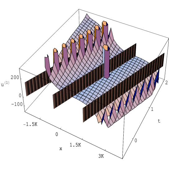
Figure 1: Class 1 travelling wave for Selection I. The primary inputs: $\alpha=0.5,\beta=0.1,k=0.7$ and the scaling parameters are $u_{0}=z_{0}=0$. The humps are the signature of singularity.

• Selection I

  Let us choose the zeros of $F^{\prime}$ as $\pm 1,\pm 1/k(0<k^{2}<1)$ which correspond to the selection of triplet $(\varepsilon_{1},\varepsilon_{2},\varepsilon_{3})=(-1,1,-k^{2})$ or $(-k^{2},1,-1)$. Choosing $z_{0}$ such that $F(z_{0})=0$, one then obtains (see Table I of [36])

  $$F(z)=\textrm{sn}(z-z_{0})\,.$$ (32)

  Thus we are led to four classes of solutions of which the first two ($j=1,2$) correspond to the singular solutions :

  $$\mbox{Class }j:\quad v^{(j)}=a_{0}+a_{2}\textrm{sn}^{2}(z-z_{0})+a_{-2}\textrm{ns}^{2}(z-z_{0})\,,$$ (33)

  where $a_{i}$s are obtained from 1st and 2nd rows of Table 1 & Table 2. The corresponding travelling wave solutions $u^{(j)}$ are obtained from the integration of (33) and involves a singularity at $z=z_{0}$ as is evident from the formula [40]

  $$\int_{0}^{z-z_{0}}\left(\textrm{ns}^{2}\tau-\frac{1}{\tau^{2}}\right)\textrm{d}\tau = z-z_{0}+\frac{1}{z-z_{0}}$$ (34)

  $$\mbox{}-E(\vartheta_{0},k)-\textrm{cn}(z-z_{0})\textrm{ds}(z-z_{0})\,.$$

  In the expression (34) and also in the following $\vartheta_{\ell}$ is defined by $\sin\vartheta_{\ell}=\textrm{sn}(z-z_{\ell},k)$ for $\ell=0,1$. In this context it is worth mentioning that in the limit $k\rightarrow 1$, the travelling wave reduces to $\coth$-type solution which also has a singularity at $z=z_{0}$. This solution was derived from a different approach in Ref. [28]. It is well known that such a singular solution may serve as a model for physical phemenon of so-called “hot-spots” [41, 42, 43].

  In the following our aim would be to find regions where the travelling wave solutions ($j=1,2$) corresponding to (33) are regular. We use the following infinite trigonometric series expansion [40] of $\textrm{ns}(z-z_{0},k)\equiv 1/\textrm{sn}(z-z_{0},k)$ :

  $$\textrm{ns}(z-z_{0},k) = \frac{\pi}{2K}\textrm{cosec}\tau$$ (35)

  $$\mbox{}-\frac{2\pi}{K}\sum_{n=0}^{\infty}\frac{q^{2n+1}}{1-q^{2n+1}}\sin[(2n+1)\tau]\,,$$

  where $q=\exp[-\pi K^{\prime}/K]$ is known as nome of the elliptic functions and $\tau=\pi(z-z_{0})/2K$, $K^{\prime}(k)=K(k^{\prime})$, the quantities $K(k)$ and $k$ have already been defined in Sec. 2. Denoting the singular term in the travelling wave solutions by the symbol $S_{0}$, we see that as $z\rightarrow z_{0}$, the asymptotic expression of its 1st term will be

  $$S_{0}(z\rightarrow z_{0})=\frac{\pi}{2K}\textrm{cosec}\tau$$ (36)

  We will now use the well known expansion for $\textrm{cosec}\tau$ convergent in the region $|\tau|<\pi$

  $$\textrm{cosec}\tau=\frac{1}{\tau}+\sum_{n=1}^{\infty}\frac{(-1)^{n-1}2(2^{2n-1}-1)B_{2n}}{(2n)!}\tau^{2n-1}\,,$$ (37)

  where $\{B_{n}\}$ are Bernoulli numbers whose first few members are $B_{0}=1,B_{1}=-1/2$, $B_{2}=1/6,B_{4}=-1/30$ etc.

  Combining (36) and (37), it is straightforward to conclude that near $z\sim z_{0}$, the travelling wave solution behaves like $(z-z_{0})^{-1}$ i. e. the point $z=z_{0}$ is a simple pole. Note that the region of convergence of the series (37) for $\textrm{cosec}\tau$ is

  $$|\tau|<\pi\Rightarrow|z-z_{0}|<2K$$ (38)

  The above equation speaks of two parallel planes

  $$x-ct-z_{0}\pm 2K=0\,,$$ (39)

  which are normal to wave surface. These two planes are shown in Fig. 1 [see two extreme strips orthogonal to surface $u=u(x,t)$]. It is thus quite expected that wave surface will be irregular along these two planes. This fact can be appreciated from the humps along the strips in Fig. 1 showing sudden rise of the value $u=u(x-ct)$. Further there must be a singularity at $z=z_{0}$. From elementary analysis we know that in $t$-$x$ plane the point $z=x-ct$ approaches point $z_{0}$ along any curve. Hence there will be a circular disc in the plane $z=z_{0}$ centred at $z_{0}$ and of arbitrary small radius where solution will show irregularity. This is reflected by a single localized hump in Fig. 1 on the plane lying parallel and midway between two extreme planes.

  To use such a solution we thus need an exact knowledge about the position of parallel humps. These may be exactly computed by the solid angles $\theta_{x}=\cos^{-1}|1/\sqrt{1+\textrm{c}^{2}}|$ and $\theta_{t}=\cos^{-1}|\textrm{c}/\sqrt{1+\textrm{c}^{2}}|$. These two angles in turn depend on the parameter c which determines the wave speed. Hence very fast and very slow waves have different regions of humps. The core singularity at $z=z_{0}$ will however be present in same region for all types of waves which may be removed by making a hole of arbitrary small radius on the plane $z=z_{0}$ around point $z_{0}$. This concludes our detailed analysis about singularity of Class 1 and 2 solutions for Selection I which hopefully provides a sufficient basis of the solution regarding its potential use.

  The other two classes correspond to the non-singular solutions

  $$\mbox{Class }j:\quad v^{(j)}=a_{0}+a_{2}F^{2}\,,\qquad j=3,4\,.$$ (40)

  The resulting travelling wave solutions are of the same form as the solutions (14) and (19) obtained in Sec 2:

  $$u^{(j)}=u_{0}+(a_{0}+\frac{a_{2}}{k^{2}})(z-z_{0})-\frac{a_{2}}{k^{2}}E(\vartheta_{0},k)\,,$$ (41)

  where $a_{i}$s are to be computed from last two rows of Table 1 and Table 2. Note that Class $4$ solution is linear in $x$ and $t$, since $a_{\pm 1}=a_{\pm 2}=0$ (see the last rows of the tables).

• Selection II

  Let us now choose pairs of purely real and of purely imaginary roots of $F^{\prime}$ respectively as $\pm 1/k^{\prime}(0<k^{\prime 2}=1-k^{2}<1)$ and $\pm i/k$ which come from the selection $(\varepsilon_{1},\varepsilon_{2},\varepsilon_{3})=(-k^{\prime 2},1,k^{2})$ or $(k^{2},1,-k^{\prime 2})$. One then obtains the following representation of $F(z)$:

  $$F(z)=\textrm{sd}(z-z_{0},k)\,,$$ (42)

  leading to a new solution of $u(z)$. The explicit expressions for Class 1 and Class 2 are given by

  $$u^{(j)} = u_{0}+\varrho_{j}(z-z_{0})-(3-j)a_{-2}E(\vartheta_{0},k)$$ (43)

  $$\mbox{}+\!(2\!-\!j)k^{2}a_{-2}\textrm{sn}(z\!-\!z_{0},k)\textrm{cd}(z\!-\!z_{0},k)\!+\!S_{0}$$

  for $j=1,2$, where we have abbreviated $\varrho_{j}$ as $\varrho_{j}=a_{0}+(3-j)k^{\prime 2}a_{-2}$. The non-singular solutions corresponding to Class 3 and 4 solutions read

  $$u^{(j)} = u_{0}+\left(a_{0}-\frac{a_{2}}{k^{2}}\right)(z-z_{0})+\frac{a_{2}}{k^{2}k^{\prime 2}}E(\vartheta_{0},k)$$ (44)

  $$\mbox{}-\frac{a_{2}}{k^{\prime 2}}\textrm{sn}(z-z_{0},k)\textrm{cd}(z-z_{0},k)\,,\>j=3,4\,.$$

  The main feature of Selection II is that the solutions coming from that are nearly periodic in the whole domain due to the additional sn and cd-term. In contrast the solutions generated from Selection I are only quasi-periodic, the periodic behaviour is observed for singular solutions which are prominent near $z\sim z_{0}$.

  

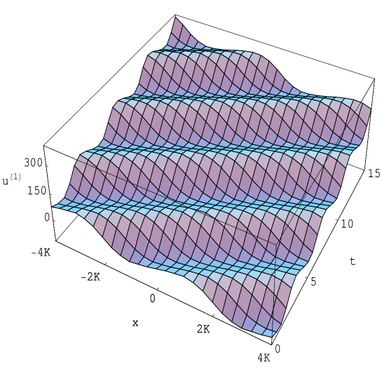
  Figure 2: Class 1 travelling wave for Selection III for the same primary inputs and scalings are $u_{1}=z_{1}=0$. The smoothness of the wave-surface shows the solution is non-singular.

• Selection III

  We just saw that the Class $1$ and $2$ solutions generate singular solutions owing to the generating functional $F(z(x,t))$ possessing either a zero or a pole in the region of validity. It is indeed possible to generate non-singular solutions for these classes, which share similar qualitative behaviour with the previous counterparts, if $F$ can be chosen to have neither zero nor a pole in the finite part. Below we provide such an example, which are the only one among the set of elliptic functions.

  We choose the zeros of $F^{\prime}$ as $\pm 1,\pm 1/k^{\prime}$ corresponding to the selection $(\varepsilon_{1},\varepsilon_{2},\varepsilon_{3})=(-k^{\prime 2},-1,1)$. Then we have the following representation of $F(z)$ (see Table I of [36])

  $$F(z)=\textrm{nd}(z-z_{1},k)\,,$$ (45)

  where $z_{1}$ is fixed as $F(z_{1})=1$. It is now trivial to check that the generated solutions for each of the four classes remain non-singular

  $$u^{(j)} = u_{1}+a_{0}(z-z_{1})+(3-j)a_{-2}E(\vartheta_{1},k)$$ (46)

  $$\mbox{}-(2\!-j)k^{2}a_{-2}\textrm{sn}(z\!-\!z_{1},k)\textrm{cd}(z\!-\!z_{1},k)\,;$$

  $$u^{(j)} = u_{1}+a_{0}(z-z_{1})+a_{2}E(\vartheta_{1},k)/k^{\prime 2}\,,$$ (47)

  $$\mbox{}-k^{2}a_{2}\textrm{sn}(z-z_{1},k)\textrm{cd}(z-z_{1},k)/k^{\prime 2}\,,$$

  where $j=1,2$ for Equation (46) and $j=3,4$ for (47). Fig. 2 depicts a Class 1 wave guided by (46).

Other possible selections from Table I of [36] will generate many such new elliptic travelling wave solutions of GSWW equation. Let us mention that the degenerate selections leading to hyperbolic and trigonometric type waves can be obtained from elliptic solutions in $k\rightarrow 0,1$ limits.

4 Summary

In this article we proposed an extended method to generate a rich class of doubly-periodic elliptic travelling wave solutions of the GSWW equation. A systematic classification is given for the solutions to exhaustively utilize the strength of the proposed method. We also discussed a canonical procedure for generating travelling wave solutions. The problem with such solutions is that these require the pre-knowledge of zeros of second derivative of the solutions. The proposed EEF method removes this difficulty by fixing the zeros of the first derivative of the solutions and leads to a wide range of travelling waves which include the kink type solitary wave [16], sinusoidal type periodic solution [27] and a rational solution ([29]). Class 1 to 4 classify the various types of solutions whose explicit forms are noted for three representative selections of integral parameters defining the generating functional. Classes 1 and 2 produce singular solutions which has important application in modelling the physical curcumstances of formation of hot-spots [41, 42, 43]. We have exactly computed the positions of such blow-up of solutions and graphically illustrated in the Fig. 1. To the best of our knowledge such an analysis about the region of blow-up for singular elliptic solutions has not been done previously in the literature.

References

- [1] Levi D and Winternitz P (Eds) 1988 Symmetries and nonlinear phenomena (WS)
- [2] Konopelchenko B G 1987 Nonlinear integrable equations (Springer-Verlag)
- [3] Léon J J-P (Ed) 1988 Nonlinear evolutions (WS)
- [4] Nayfeh A H and Balachandran B 1995 Applied nonlinear dynamics: Analytical, Computational and Experimental Methods (Willey-Interscience NY)
- [5] Baldwin D and Hereman W 2010 “A symbolic algorithm for computing recursion operators of nonlinear PDE’s” Int. J. Computer Mathematics (in press)
- [6] Wiggins S 2003 Introduction to Applied Nonlinear Dynamical systems and Chaos (Springer)
- [7] Guha-Roy C 1989 Some studies of solitons and solitary waves in nonlinear systems (Thesis J.U.)
- [8] Mobius P. 1987 Czech. J. Phys. B 37 1041
- [9] Makhankov V G 1978 Phys. Rep. 35 1
- [10] Zakharov V E and Shabat A B 1974 Func. Anal. Appl. 8 226
- [11] Lax P D 1968 Comm. Pure. Appl. Math. 21 467
- [12] Wahlquist H D and Estabrook F B 1973 Phys. Rev. Lett. 31 1386
- [13] Hirota R and Satsuma J 1981 Phys. Lett. A 85 407
- [14] Satsuma J and Hirota R 1982 J. Phys. Soc. Japan 51 332
- [15] Whitham B 1974 Linear and Nonlinear Waves (Willey-Interscience, NY)
- [16] Miura R M, Gardner C S and Kruskal M D 1968 J. Math. Phys. 9 1204
- [17] Malfliet W and Hereman W 1996 Phys Scripta 54 563, 569
- [18] Wazwaz A-M 2009 Appl. Maths. and Computation 212 120
- [19] Wang M L 1995 Phys. Lett. A 199 169
- [20] Wazwaz A M 2004 Math. and Comput. Modelling 40 499
- [21] Yan C T 1996 Phys. Lett. A 224 77
- [22] Wang M L 2003 Phys. Lett. A 318 84
- [23] Yomba E 2005 J. Math. Phys. 46 123504
- [24] Wang M, Li X and Zhang J 2008 Phys. Lett. A 372 417
- [25] Fan E 2002 J. Phys. A 35 6853
- [26] Hietarinta J 1990 Partially integrable Evolution Equations in Physics ed R Conte and N Boccara NATO ASI Series C: Mathematical and Physical sciences 310 (Dordrecht: Kluwer) 459
- [27] Clarkson M. A. and Mansfield E. L. 1994 Nonlinearity 7 975
- [28] Elwakil S A, El-labany S K, Zahran M A and Sabry R 2003 Chaos Solitons Fractals 17 121
- [29] Drazin P G and Johnson R S 1983 Solitons: An Introduction (London: Cambridge University press)
- [30] Yomba E 2010 Phys Lett. A, doi: 10.1016/j.physleta.2010.02.026
- [31] Chen H, Zhang H 2003 Chaos Solitons Fractals 15 585
- [32] Andreev V A and Burova M V 1990 Theor. Math. Phys. 85 376
- [33] Andreev V A and Shmakova M V 1993 J. Math. Phys. 34 3491
- [34] Bagchi B, Lahiri A and Roy P K 1989 Phys. Rev. D 39 1186
- [35] Bagchi B, Beckers J and Debergh N 1998 Int. J. Mod. Phys. A 13 3203
- [36] Ganguly A 2002 J. Math. Phys 43 1980
- [37] Khater A H, Malfliet W, Callebaut D K and Kamel E S 2002 Chaos Solitons Fractals 14(2) 513
- [38] Fu Z T, Liu S K, Liu S D, Zhao Q 2001 Phys. Lett. A 290 72
- [39] Yusufoğlu E, Bekir A 2007 Int. Jour. of Nonlinear Sci. 4 10
- [40] Abramoitz M, Stegun A 1972 Handbook of Mathematical functions (National Bureau of Standards, USA, Applied Math. series 55)
- [41] Smyth NF 1992 J. Aust. Math. Soc. Ser B33 403
- [42] Clarkson PA and Mansfield EL 1993 Physica D 70 250
- [43] Kudryashov NA and Zargayan D 1996 J. Phys. A 29 8067