Direct observation of a sharp transition to coherence in Dense Cores

Abstract

We present ${\rm NH_{3}}$ observations of the B5 region in Perseus obtained with the Green Bank Telescope (GBT). The map covers a region large enough ($\sim$11′$\times$14′) that it contains the entire dense core observed in previous dust continuum surveys. The dense gas traced by ${\rm NH_{3}}$(1,1) covers a much larger area than the dust continuum features found in bolometer observations. The velocity dispersion in the central region of the core is small, presenting subsonic non-thermal motions which are independent of scale. However, it is thanks to the coverage and high sensitivity of the observations that we present the detection, for the first time, of the transition between the coherent core and the dense but more turbulent gas surrounding it. This transition is sharp, increasing the velocity dispersion by a factor of 2 in less than 0.04 pc (the 31$\arcsec$ beam size at the distance of Perseus, $\sim$250 pc). The change in velocity dispersion at the transition is $\approx 3~{}{\rm km\,s^{-1}\,pc^{-1}}$. The existence of the transition provides a natural definition of dense core: the region with nearly-constant subsonic non-thermal velocity dispersion. From the analysis presented here we can not confirm nor rule out a corresponding sharp density transition.

1. Introduction

The velocity dispersion in molecular clouds (MCs) has been known for years to be supersonic. Several numerical simulations of supersonic turbulence can successfully reproduce some of the MCs properties. But, dense cores, where stars are actually formed, present velocity dispersions with non-thermal motions smaller than the thermal values and also independent of scale (Goodman et al., 1998; Caselli et al., 2002). Goodman et al. (1998) and Caselli et al. (2002) coined the term “coherent core,” to describe the region where the non-thermal motions are subsonic and constant as “islands of calm in a more turbulent sea.” Goodman et al. (1998) showed that the lower density gas around cores, traced by OH and C¹⁸O (1–0), presents supersonic velocity dispersions that decrease with size, as expected in a turbulent flow, while the dense gas associated with cores traced by ${\rm NH_{3}}$ shows a nearly-constant, nearly-thermal width. Therefore, a transition between turbulent gas and more quiescent gas must happen at some point. However, it was not clear if the transition could be detected in the dense gas tracer on its own and/or if it is a smooth or abrupt transition.

The nearby Perseus MC, at $\sim$250 pc, is a good place to search for the transition to coherence. A large number of “dense cores” have been identified in dust continuum surveys (Hatchell et al., 2005; Enoch et al., 2006; Kirk et al., 2006), and previous ${\rm NH_{3}}$ observations have been carried out Rosolowsky et al. (2008); Ladd et al. (1994); Benson & Myers (1989). From these core lists, B5 stands out as a rather isolated and bright dense core that has been studied in detail in the past (Young et al., 1982; Langer et al., 1989; Fuller et al., 1991; Bally et al., 1996; Bensch, 2006; Pineda et al., 2008), with $\approx 11\,M_{\odot}$ detected in dust continuum. It should be noted that dense cores are usually identified as objects which are detected in some molecular line emission tracing dense gas, e.g., ${\rm NH_{3}}$(1,1) or ${\rm N_{2}H^{+}}$(1–0), or in dust continuum, e.g., MAMBO, SCUBA, BOLOCAM, LABOCA. But, it is not clear that different tracers and instruments provide a consistent object definition.

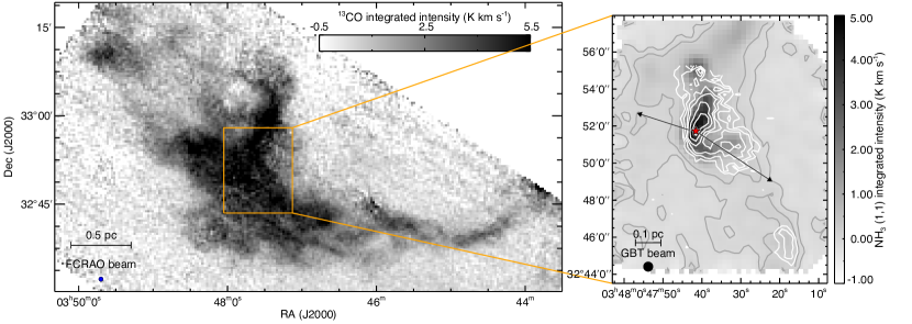
Figure 1.— Left panel: Map of ${\rm{}^{13}CO}$(1–0) integrated intensity for the B5 region obtained by the COMPLETE Survey (Ridge et al., 2006). The orange box shows the area mapped with the GBT. Right panel: Integrated intensity map of B5 in ${\rm NH_{3}}$(1,1). White contours are BOLOCAM dust continuum emission (Enoch et al., 2006), while gray contours show the 0.15 and 0.3 ${\rm K\,km\,s^{-1}}$ level in ${\rm NH_{3}}$(1,1) integrated intensity. The young star, B5–IRS1, is shown by the star. The outflow direction is shown by the arrows.

If velocity dispersion and density profiles are related, then a transition should also be seen in column density. For this at least two well known techniques could be used: extinction maps and dust continuum emission maps. Extinction maps trace the total column density along the line of sight, and they are useful to study the large scale structure in MCs (e.g., Lada et al., 1994; Alves et al., 1998; Lombardi & Alves, 2001; Pineda et al., 2008; Goodman et al., 2009) and to identify dense cores (e.g., Alves et al., 2007). Unfortunately, the coarse angular resolution achieved in extinction maps ($\geq 1\arcmin$) is still not quite enough to allow detailed studies of the column density structure within and around cores, with the exception of only a handful of cases e.g., B68 (Alves et al., 2001). Dust continuum observations using SCUBA (Hatchell et al., 2005; Kirk et al., 2006), MAMBO (Motte et al., 1998; Kauffmann et al., 2008) and SHARC II (Li et al., 2007) have angular resolution of 15$\arcsec$, 11$\arcsec$ and 9$\arcsec$, respectively, which are high enough to enable the study of the transition to coherence. However, due to observing techniques (sky removal and/or chopping), they filter out large-scale emission (usually between 1.5$\arcmin$ and 2$\arcmin$), and therefore dust continuum maps are not suitable to study the region where the transition to coherence happens. Currently, these limitations on dust mapping leaves high-resolution, spatially-unfiltered, molecular line observations as the best tool to look for the “environs” to “core” transition.

In this letter, we present new ${\rm NH_{3}}$ observations of B5 obtained with the 100-m Robert F. Byrd Green Bank Telescope (GBT) which provide the first detection of the transition to coherence in a single tracer. These observations provide answers to two questions: a) what is the extent of coherent dense cores?; and b) is the transition to coherence smooth or abrupt?

2. Data

We observed B5 using the GBT. The observations were carried out between December 23 and March 31, 2009 (project 08C-088), using the On-The-Fly (OTF) technique (Mangum et al., 2007), with a dump rate of 3 dumps per beam, and producing a dump every 3 seconds.

We used the high-frequency K-band receiver and configured the spectrometer to observe four 12.5 MHz windows centered on ${\rm NH_{3}}$(1,1), ${\rm NH_{3}}$(2,2), CCS ($2_{1}$–$1_{0}$) and HC₅N (9–8) rest frequencies. We chose to use two feeds and two polarizations simultaneously, which trades decreased spectral resolution for increased sensitivity given GBT spectrometer constraints. The spectrometer generated 4096 lags across each window, giving a 3.050 kHz channel separation, equivalent to $0.04~{}{\rm km\,s^{-1}}$ for the ${\rm NH_{3}}$ spectra. We observed in frequency switching mode, with a shift of 2.0599365 MHz around the center of the band. This configuration ensured that all 18 hyperfine components of ${\rm NH_{3}}$(1,1) were observed within the spectral window. The pointing model was updated every 60–90 minutes, depending on weather conditions, using the quasar 0336+3218. Flux calibration was carried out by observing the flux calibrator 3C 48 during each session. All the intensities reported here are on the $T_{A}^{*}$ scale, which is established using atmospheric opacity estimates at 22–23 GHz. Data cubes are generated using all observations taken and convolved onto a common grid with a tapered Bessel function (see Mangum et al., 2007). The GBT main beam efficiency ($\eta_{mb}$) is 0.81 at these frequencies. All the data reduction was carried out in GBTIDL. The median rms in the map is 0.046 K.

The resulting ${\rm NH_{3}}$(1,1) integrated intensity map for B5 is shown in Figure 1, and it covers a region of size 11$\arcmin\times$14$\arcmin$. Gray contours in Figure 1 show the extension of ${\rm NH_{3}}$(1,1) emission.

3. Results

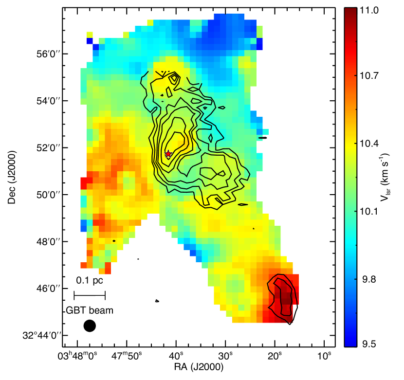
Figure 2.— Centroid velocity map of B5 obtained by fitting the ${\rm NH_{3}}$ lines. The position of the protostar is shown by the star. Black contours are Bolocam dust continuum emission (Enoch et al., 2006). The GBT beam size is shown at the bottom left.

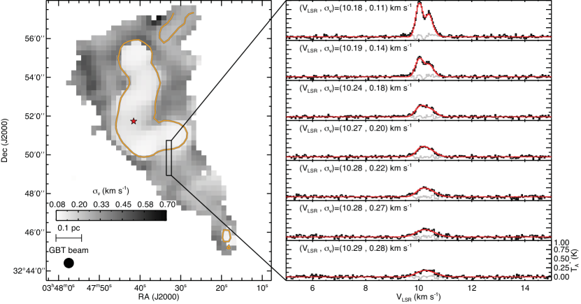
Figure 3.— Velocity dispersion map derived from fitting all hyperfine components simultaneously. The protostar position is shown by the star, and the contour shows the contour $T_{peak}=0.5$ K. The box on the map presents the region where we zoom in and present the corresponding spectra in the right panel, which shows only the main component of the ${\rm NH_{3}}$(1,1) line. The centroid velocity and velocity dispersion obtained from the fit is displayed for each position. Top spectra in the right panel display two main hyperfine components clearly separated thanks to their low velocity dispersion (the coherent core), while when moving to positions outside the core the lines get weaker and broader (evident by the disappearance of the gap between hyperfine components).

The ${\rm NH_{3}}$(1,1) and (2,2) lines are fitted simultaneously using a forward model as in Rosolowsky et al. (2008). This method allows us to obtain centroid velocity ($v_{LSR}$), velocity dispersion ($\sigma_{v}$), kinetic temperature ($T_{k}$), excitation temperature ($T_{ex}$) and opacity ($\tau_{11}$) for every position, while also including the response of the frequency channel using a sinc profile. If the ${\rm NH_{3}}$(1,1) line is optically thin then $\tau_{11}$ and $T_{ex}$ can not be obtained independently, and therefore the optically thin approximation is used if $\tau_{11}<1$ or $\sigma_{\tau_{11}}<0.4\,\tau_{11}$, where $\sigma_{\tau_{11}}$ is the optical depth uncertainty (obtained from the fit). The centroid velocity map is shown in Figure 2 for positions where ${\rm NH_{3}}$(1,1) is detected. When compared to dust emission maps from BOLOCAM (see contours in Figures 1 and 2) or SCUBA, we find that the ${\rm NH_{3}}$(1,1) emission is spatially more extended than its dust continuum counterpart. Therefore, dense gas traced by ${\rm NH_{3}}$(1,1) is detected outside the boundaries of the dust-defined “dense core,” calling into question the accuracy of dense core classification based only on the detection of a high-density tracer.

Since our subsequent analysis of $\sigma_{v}$ depends on very high accuracy, we eliminate from further consideration positions that do not fulfill the following criteria: a) clear detection of ${\rm NH_{3}}$(1,1); b) $\sigma_{\sigma_{v}}<0.05~{}{\rm km\,s^{-1}}$; and c) $\sigma_{\sigma_{v}}<0.2\,\sigma_{v}$; where $\sigma_{\sigma_{v}}$ is the $\sigma_{v}$ uncertainty from the fit. These conservative criteria eliminate observations where the velocity dispersion are poorly determined. The velocity dispersion map for B5 is presented in Figure 3. From this map it is clear that the central part of the core presents a region with small and uniform velocity dispersion. However, outside of this region there is extended ${\rm NH_{3}}$(1,1) emission with much larger velocity dispersion, as large as a four times the velocity dispersion found within the core. Therefore, we have observed for the first time in a single tracer the transition between dense but turbulent gas into more quiescent dense gas. A more detailed view of the transition is shown in the right panel of Figure 3, which displays only the main hyperfine blend of ${\rm NH_{3}}$(1,1) along a vertical cut marked by the vertical box in the left panel, and where the gap between hyperfine components disappear for broader lines. The transition appears to be sharp at GBT resolution, occurring over just one beam width (two 15.5$\arcsec$ pixels). Using a 250 pc distance to Perseus, the 31$\arcsec$ beam gives a 0.04 pc upper limit to the transition scale.

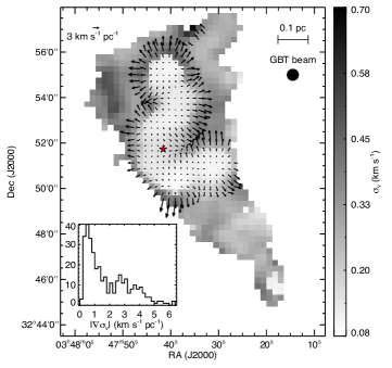
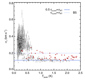
Figure 4.— Left panel: Velocity dispersion map in the background. The young star, B5–IRS1, is shown by the star. The velocity dispersion gradient is shown by the arrows. The inset shows the velocity dispersion gradient distribution. The narrow peak at low values are the positions within the coherent core, while the transition surface populates the second distribution of points at larger values. Right panel: Velocity dispersion as a function of peak antenna temperature ($T_{peak}$). Red points are positions with a distance to B5–IRS1 smaller than 2.025 times the GBT beam. The peak antenna temperature can be used as a proxy of distance from the center, where high $T_{peak}$ are found close to the center of the core and low $T_{peak}$ are found are larger distances. Notice the small dispersion in $\sigma_{v}$ at high $T_{peak}$ (the coherent core) consistent with subsonic non-thermal components, and the abrupt increase in $\sigma_{v}$ when approaching the transition to coherence with supersonic non-thermal components. The dispersion in $\sigma_{v}$ within the coherent core is even smaller after considering that the red points are affected by the central YSO. Blue horizontal lines show the expected velocity dispersion for two values of the velocity dispersion non-thermal component ($\sigma_{NT}$): $0.5\,{\rm c_{s,ave}}$, and ${\rm c_{s,ave}}$, where ${\rm c_{s,ave}}$ is the sound speed of the average particle ($\mu=2.33$) assuming ${\rm T_{kin}}$=10 K.

To better characterize the transition between turbulent and calm gas, we map out the local gradient in $\sigma_{v}$ over B5. The distribution of this gradient’s absolute value, $|\nabla\sigma_{v}|$, is shown as an inset histogram in Figure 4. (Note that only positions marked by arrows in the Figure’s grey scale map of $\sigma_{v}$ are included in the histogram.) The orientation of $\nabla\sigma_{v}$ at the transition is almost perpendicular to it, while inside the coherent core it is close to randomly oriented. The gradient amplitude distribution exhibits two peaks, with a narrow peak at small dispersion coming from within the coherent core. For the region in and immediately surrounding the coherent core in B5 (where arrows are shown in Figure 4), a typical value of 3 ${\rm km\,s^{-1}\,pc^{-1}}$ for $|\nabla\sigma_{v}|$ is found. Combining this typical value of $|\nabla\sigma_{v}|$ with the difference between the median velocity dispersion for positions with subsonic and supersonic non-thermal motions (0.32 ${\rm km\,s^{-1}}$ and 0.13 ${\rm km\,s^{-1}}$, respectively) we estimate a transition physical scale of 0.06 pc. This estimate of the transition scale is actually also an upper limit, because it does not take into account that the observations are smoothed by the telescope beam (0.04 pc at the distance of Perseus).

In the right panel of Figure 4 we show the velocity dispersion as a function of peak antenna temperature ($T_{peak}$). Points marked in red are at a distance smaller than 63$\arcsec$ from the embedded YSO in B5 and likely have increased velocity dispersion as a result. If the peak antenna temperature is used as a proxy for the distance from the core center (as in Barranco & Goodman, 1998; Goodman et al., 1998), then it is clear that close to the center of the core velocity dispersions are small and display a small spread (the coherent zone). At lower $T_{peak}$ (larger radii) there is a sudden increase in $\sigma_{v}$. Notice that the uncertainty in the dispersions is comparable to the symbol size at $T_{peak}>0.7$ K, and still relatively small even at the lowest intensities analyzed here. To re-assure ourselves that there is no bias in our fitting toward finding higher dispersion for weak lines, we performed tests on synthetic data, and found no bias that could explain the trend in Figure 4. In fact, because the integrated intensity ($\propto T_{peak}\,\sigma_{v}$) map is smooth (most likely due to a smooth column density profile) $T_{peak}$ must rapidly decrease to compensate for the sharp transition in $\sigma_{v}$. This very simple argument can explain the effect seen in Figure 4, however, it does not provide an answer to the origin of the velocity dispersion transition.

4. Discussion

The detection of a sharp transition to coherence provides very stringent constraints on numerical models of dense cores. Certainly the study of the density structure is important to understand the relation between the core and its environment, and also to study the relation between density and velocity dispersion (e.g. Myers & Fuller, 1992), however, such a discussion is beyond the scope of this letter. Here, we present a transition in velocity dispersion, for which we can not confirm nor rule-out an analogous density transition.

The presence of the sharp transition allows for a robust definition of a coherent dense core: a region with nearly-constant subsonic non-thermal motions. Most certainly, the proposed approach of using the transition to coherence to define a dense core is not as time-efficient as using only large format bolometers, but it provides an identification system that is based on a physical quantity, and therefore it should be consistent with more sensitive observations. In the future, when more observations of the transition to coherence in molecular lines are available for cores also mapped in dust, it might (or might not!) be possible to develop an empirical relation to improve the coherent cores identification using only dust maps.

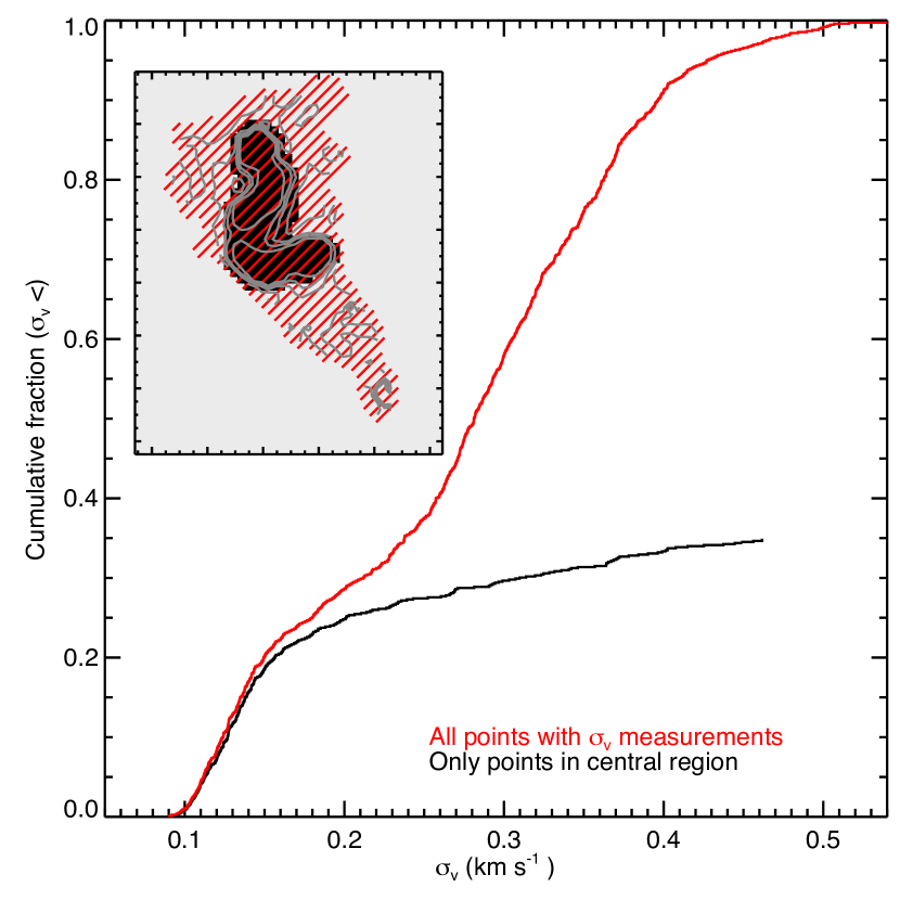
Figure 5.— Velocity dispersion cumulative distribution. Red curve shows the cumulative distribution for all points with good velocity dispersion measurements, while the black curve uses only points close to the central core. The sharp transition in velocity dispersion produces a change in the cumulative distribution’s slope, which can be observed both locally (central region) and globally (entire map). The inset shows the spatial distribution of the points used, and velocity dispersion contours are overlaid in gray.

The velocity dispersion cumulative distribution is shown in Figure 5. The transition to coherence is a distinct feature in the cumulative distribution, where a change in slope is clearly observed. The effect is not only local, but it is also evident in the cumulative distribution for the entire region. Moreover, the velocity dispersion at which the cumulative distribution slope changes is robust against variations in the region selected to generate the cumulative function.

A study comparing kinetic temperature and velocity dispersion across the transition would be important to understand its origin. However, outside the coherent core, increases in velocity dispersion are accompanied by decreases in line brightness. In our present GBT data set, the ${\rm NH_{3}}$(2,2) emission beyond the transition to coherence cannot be reliably mapped because of the weaker lines. Since both (1,1) and (2,2) measurements are needed to determine kinetic temperature, we can not yet study how temperature varies across the transition.

Alves et al. (2001) showed that the column density profile of B68 can be well modeled by a Bonnert-Ebert (BE) sphere. Since then, this analysis has been applied to more cores finding that it usually is a good description (e.g., Kandori et al., 2005), although we do not try to model B5 as a BE sphere. However, a column density profile similar to BE can also be obtained in more dynamic events (e.g. Myers, 2005; Gómez et al., 2007). Lada et al. (2008) argued that most of the cores in the Pipe can be pressure confined by the MC’s own weight, see also Bertoldi & McKee (1992) and Johnstone et al. (2004). The observed increase in the velocity dispersion might be evidence for a pressure difference between the coherent core and the external medium. However, in all these cases there is no explanation or description of what happens at the core boundary: is there a discontinuity? or is it a smooth transition with the background?

The presence of a sharp transition to coherence suggests shock and/or instability/fragmentation origins. Shocks are predicted in models of core formation in supersonic flows (Padoan et al., 1997) and in models of colliding large-scale flows, e.g. Heitsch et al. (2005). Core formation simulations (1D) from converging supersonic flows (Gómez et al., 2007; Gong & Ostriker, 2009) predict a density and velocity discontinuity at the (isothermal) shock front position, which would also provide a core definition. Unfortunately, there is no discussion of the spatial dependence of the resulting velocity dispersion (see Heitsch et al., 2009, for large scale velocity dispersion maps in colliding flows).

Klessen et al. (2005) argue that coherent cores can also be formed by gravo-turbulent fragmentation of molecular cloud material. Klessen et al. (2005) show the velocity dispersion map for some cores in all three projections, and from these figures an abrupt increase in velocity dispersion can be identified (somewhat in agreement with our observations). However, there are important discrepancies between the results from Klessen et al. (2005) and the observations:

1. The increase in velocity dispersion observed in ${\rm NH_{3}}$(1,1) surrounds the entire coherent dense core, with broader lines systematically found outside the coherent dense core. While Klessen et al. (2005) finds an increase in the velocity dispersion in more confined regions (such as a ring around or a stripe next to the coherent core) and with narrow velocity dispersions found past these features.

2. Foster et al. (2009) shows that 81 out of the 83 cores in Perseus observed by Rosolowsky et al. (2008) display subsonic non-thermal motions at their center, while in Klessen et al. (2005) only a 12–52% of the identified objects (which depends on the nature of the driving mechanism) display coherent subsonic non-thermal motions.

Moreover, it is not clear if any of the models discussed above can predict the transition to coherence at densities high enough to be observed in ${\rm NH_{3}}$(1,1). In the case of cores formed from shocks this constraint could be extremely important, because the density enhancement generated by the shock front can be large enough (a factor of $\approx\mathcal{M}^{2}$, where $\mathcal{M}$ is the Mach number) to make the detection of ${\rm NH_{3}}$(1,1) outside the coherent core difficult for highly supersonic turbulence.

Previous attempts to constrain numerical simulations of dense cores using single-pointing surveys of dense gas (e.g., Kirk et al., 2007; Rosolowsky et al., 2008) result in loose constraints on simulations (Offner et al., 2008; Kirk et al., 2009). In Offner et al. (2008), they present velocity dispersion maps derived from synthetic ${\rm NH_{3}}$(1,1) observations for some cores which do not show a velocity dispersion increase similar to the one presented in this letter. Clearly these new observations allow us to place a different set of constraints on numerical simulations that might help to improve the initial conditions assumed for star formation. Therefore, it is now the turn of simulators to produce synthetic observations from their simulations that can be compared with those presented here.

References

- Alves et al. (1998) Alves, J., Lada, C. J., Lada, E. A., Kenyon, S. J., & Phelps, R. 1998, ApJ, 506, 292
- Alves et al. (2007) Alves, J., Lombardi, M., & Lada, C. J. 2007, A&A, 462, L17
- Alves et al. (2001) Alves, J. F., Lada, C. J., & Lada, E. A. 2001, Nature, 409, 159
- Bally et al. (1996) Bally, J., Devine, D., & Alten, V. 1996, ApJ, 473, 921
- Barranco & Goodman (1998) Barranco, J. A., & Goodman, A. A. 1998, ApJ, 504, 207
- Bensch (2006) Bensch, F. 2006, A&A, 448, 1043
- Benson & Myers (1989) Benson, P. J., & Myers, P. C. 1989, ApJS, 71, 89
- Bertoldi & McKee (1992) Bertoldi, F., & McKee, C. F. 1992, ApJ, 395, 140
- Caselli et al. (2002) Caselli, P., Benson, P. J., Myers, P. C., & Tafalla, M. 2002, ApJ, 572, 238
- Enoch et al. (2006) Enoch, M. L., Young, K. E., Glenn, J., Evans, II, N. J., Golwala, S., Sargent, A. I., Harvey, P., Aguirre, J., Goldin, A., Haig, D., Huard, T. L., Lange, A., Laurent, G., Maloney, P., Mauskopf, P., Rossinot, P., & Sayers, J. 2006, ApJ, 638, 293
- Foster et al. (2009) Foster, J. B., Rosolowsky, E. W., Kauffmann, J., Pineda, J. E., Borkin, M. A., Caselli, P., Myers, P. C., & Goodman, A. A. 2009, ApJ, 696, 298
- Fuller et al. (1991) Fuller, G. A., Myers, P. C., Welch, W. J., Goldsmith, P. F., Langer, W. D., Campbell, B. G., Guilloteau, S., & Wilson, R. W. 1991, ApJ, 376, 135
- Gómez et al. (2007) Gómez, G. C., Vázquez-Semadeni, E., Shadmehri, M., & Ballesteros-Paredes, J. 2007, ApJ, 669, 1042
- Gong & Ostriker (2009) Gong, H., & Ostriker, E. C. 2009, ApJ, 699, 230
- Goodman et al. (1998) Goodman, A. A., Barranco, J. A., Wilner, D. J., & Heyer, M. H. 1998, ApJ, 504, 223
- Goodman et al. (2009) Goodman, A. A., Pineda, J. E., & Schnee, S. L. 2009, ApJ, 692, 91
- Hatchell et al. (2005) Hatchell, J., Richer, J. S., Fuller, G. A., Qualtrough, C. J., Ladd, E. F., & Chandler, C. J. 2005, A&A, 440, 151
- Heitsch et al. (2009) Heitsch, F., Ballesteros-Paredes, J., & Hartmann, L. 2009, ApJ, 704, 1735
- Heitsch et al. (2005) Heitsch, F., Burkert, A., Hartmann, L. W., Slyz, A. D., & Devriendt, J. E. G. 2005, ApJ, 633, L113
- Johnstone et al. (2004) Johnstone, D., Di Francesco, J., & Kirk, H. 2004, ApJ, 611, L45
- Kandori et al. (2005) Kandori, R., Nakajima, Y., Tamura, M., Tatematsu, K., Aikawa, Y., Naoi, T., Sugitani, K., Nakaya, H., Nagayama, T., Nagata, T., Kurita, M., Kato, D., Nagashima, C., & Sato, S. 2005, AJ, 130, 2166
- Kauffmann et al. (2008) Kauffmann, J., Bertoldi, F., Bourke, T. L., Evans, II, N. J., & Lee, C. W. 2008, A&A, 487, 993
- Kirk et al. (2009) Kirk, H., Johnstone, D., & Basu, S. 2009, ApJ, 699, 1433
- Kirk et al. (2006) Kirk, H., Johnstone, D., & Di Francesco, J. 2006, ApJ, 646, 1009
- Kirk et al. (2007) Kirk, H., Johnstone, D., & Tafalla, M. 2007, ApJ, 668, 1042
- Klessen et al. (2005) Klessen, R. S., Ballesteros-Paredes, J., Vázquez-Semadeni, E., & Durán-Rojas, C. 2005, ApJ, 620, 786
- Lada et al. (1994) Lada, C. J., Lada, E. A., Clemens, D. P., & Bally, J. 1994, ApJ, 429, 694
- Lada et al. (2008) Lada, C. J., Muench, A. A., Rathborne, J., Alves, J. F., & Lombardi, M. 2008, ApJ, 672, 410
- Ladd et al. (1994) Ladd, E. F., Myers, P. C., & Goodman, A. A. 1994, ApJ, 433, 117
- Langer et al. (1989) Langer, W. D., Wilson, R. W., Goldsmith, P. F., & Beichman, C. A. 1989, ApJ, 337, 355
- Li et al. (2007) Li, D., Velusamy, T., Goldsmith, P. F., & Langer, W. D. 2007, ApJ, 655, 351
- Lombardi & Alves (2001) Lombardi, M., & Alves, J. 2001, A&A, 377, 1023
- Mangum et al. (2007) Mangum, J. G., Emerson, D. T., & Greisen, E. W. 2007, A&A, 474, 679
- Motte et al. (1998) Motte, F., Andre, P., & Neri, R. 1998, A&A, 336, 150
- Myers (2005) Myers, P. C. 2005, ApJ, 623, 280
- Myers & Fuller (1992) Myers, P. C., & Fuller, G. A. 1992, ApJ, 396, 631
- Offner et al. (2008) Offner, S. S. R., Krumholz, M. R., Klein, R. I., & McKee, C. F. 2008, AJ, 136, 404
- Padoan et al. (1997) Padoan, P., Nordlund, A., & Jones, B. J. T. 1997, MNRAS, 288, 145
- Pineda et al. (2008) Pineda, J. E., Caselli, P., & Goodman, A. A. 2008, ApJ, 679, 481
- Ridge et al. (2006) Ridge, N. A., Di Francesco, J., Kirk, H., Li, D., Goodman, A. A., Alves, J. F., Arce, H. G., Borkin, M. A., Caselli, P., Foster, J. B., Heyer, M. H., Johnstone, D., Kosslyn, D. A., Lombardi, M., Pineda, J. E., Schnee, S. L., & Tafalla, M. 2006, AJ, 131, 2921
- Rosolowsky et al. (2008) Rosolowsky, E. W., Pineda, J. E., Foster, J. B., Borkin, M. A., Kauffmann, J., Caselli, P., Myers, P. C., & Goodman, A. A. 2008, ApJS, 175, 509
- Young et al. (1982) Young, J. S., Goldsmith, P. F., Langer, W. D., Wilson, R. W., & Carlson, E. R. 1982, ApJ, 261, 513