HD 65949: Rosetta Stone or Red Herring

Abstract

HD 65949 is a late B star with exceptionally strong Hg II $\lambda$3984, but it is not a typical HgMn star. The Re II spectrum is of extraordinary strength. Abundances, or upper limits are derived here for 58 elements based on a model with $T_{\rm eff}=13100$K, and $\log(g)=4.0$. Even-Z elements through nickel show minor deviations from solar abundances. Anomalies among the odd-Z elements through copper are mostly small. Beyond the iron peak, a huge scatter is found. Enormous enhancements are found for the elements rhenium through mercury (Z = 75–80). We note the presence of Th III in the spectrum. The abundance pattern of the heaviest elements resembles the N=126 r-process peak of solar material, though not in detail. An odd-Z anomaly appears at the triplet (Zr Nb Mo), and there is a large abundance jump between Xe (Z = 54) and Ba (Z = 56). These are signatures of chemical fractionation.

We find a significant correlation of the abundance excesses with second ionization potentials for elements with Z $>$ 30. If this is not a red herring (false lead), it indicates the relevance of photospheric or near-photospheric processes. Large excesses (4-6 dex) require diffusion from deeper layers with the elements passing through a number of ionization stages. That would make the correlation with second ionization potential puzzling. We explore a model with mass accretion of exotic material followed by the more commonly accepted differentiation by diffusion. That model leads to a number of predictions which challenge future work.

New observations confirm the orbital elements of Gieseking and Karimie, apart from the systemic velocity, which has increased. Likely primary and secondary masses are near 3.3 and 1.6 $M_{\odot}$, with a separation of ca. 0.25 AU.

New atomic structure calculations are presented in two appendices. These include partition functions for the first through third spectra of Ru, Re, and Os, as well as oscillator strengths in the Re II spectrum.

1 Toward an understanding of CP stars

In situ chemical separation, under gravitational and radiative forces is accepted as the basic explanation of abundance anomalies in upper main sequence, chemically peculiar (CP) stars. Nevertheless, there have been few breakthroughs of the stature of arguments originally posed by Michaud (1970). Briefly, these were that the anomalies appeared in the stable atmospheres of slowly rotating stars with radiative envelopes. Additionally, the more abundant elements, helium, carbon, nitrogen, and oxygen could have little radiative support because their strong lines would be saturated. Time has not dimmed the relevance of that insight.

Scientific breakthroughs often hinge on the location of special cases, where the effects under consideration are large. A code breaker is at a severe disadvantage when faced with a brief message. With a long message, it is more likely that the regularities of a language will lead to a decryption key. We hope that the present study represents a kind of longer message, and can serve as a Rosetta stone, for an understanding of the more bizarre anomalies seen in CP stars. We provide information on more elements (58) than in a typical study of similar stars (20-30). Additionally, a number of the anomalies are very large.

The extensive analysis of Castelli and Hubrig (2004, CH04) provides a guide for the present work. Their study of the classical HgMn star, HR 7143 (HD 175640), reported abundances for 40 elements. The abundance anomalies are similar in some ways to those of HD 65949, and dissimilar in others. It has been helpful to compare results for the two stars. A detailed comparison with HR 7143 has been possible because of the spectra posted on Castelli’s (2009) web site.

The HgMn star $\chi$ Lup has also been the subject of intensive study (cf. Wahlgren 2005, and many cited references therein). The star is significantly cooler ($T_{\rm eff}=10650$K) than HD 65949 (ca. 13100K), and many important results were obtained from Hubble Space Telescope ($HST$) observations for which there is no comparable material for HD 65949. We briefly discuss the $\chi$ Lup abundances in the light of the present study.

2 An unusual late-B spectrum

Abt and Morgan (1969) noted the great strength of Hg ii $\lambda$3984 in the spectrum of HD 65949, and remarked that it did not seem to be an HgMn star. Hubrig et al. (2006) reported a weak magnetic field which might indicate a relation to the magnetic sequence of CP stars (Preston 1974).

More recent high-resolution ESO observations revealed a truly unusual spectrum (Cowley et al. 2006, Paper I, Cowley, Hubrig, & Wahlgren 2008, Paper II). In addition to the possibly record-setting strength of Hg ii $\lambda$3984, along with strong Pt ii, lines of Os ii and especially Re ii were numerous. Osmium and rhenium have been investigated in the ultraviolet spectrum of $\chi$ Lup (Wahlgren et al. 1997, Ivarsson et al. 2004), but the presence of lines of these elements in ground-based spectra is unusual.

The richness of the line spectrum is due not only to the unusual abundances. The lines are extremely sharp. We estimate from spectral synthesis, that $v\cdot\sin{i}=0.5\pm 0.5$ km s^-1.

The present work is a more complete abundance analysis of HD 65949, though based primarily on equivalent widths. For rich spectra, such as Fe i and ii, we obtained, hopefully, a sufficient number of measurements, but did not attempt to analyze all possibly relevant features. In this respect, the CH04 work is undoubtedly superior, since the entire spectrum of HR 7143 was synthesized. However, relatively small errors in the present analysis are less important than they might otherwise be, given the large departures of many values from the standard (solar) abundance distribution (SAD, e.g. Asplund, Grevesse, Sauval, and Scott 2009).

HD 65949 is located in the young cluster NGC 2516, which is known for more than a typical number of CP stars. This cluster also has an unusual number of X-ray sources (Wolk et al. 2004). These facts make it tempting to suggest that mass transfer might be relevant for some aspect of the anomalies. This is an old idea, which Wahlgren et al. (1995) remarked “remains a distant alternative, but possibly a collaborator to diffusion theory.”

3 The atmosphere of HD 65949

The effective temperature of HD 65949 is uncertain by several hundred degrees. The estimate used in Paper I, $T_{\rm eff}=13600$K, came from averaged Strömgren and H$\beta$ photometry (Hauck & Mermilliod 1998), and the calibration of Moon and Dworetsky (1985) and implemented by Moon (1984). We used a version of the Moon code kindly supplied by Dr. B. Smalley. For Paper ii, we adopted a temperature 1000K lower, which gave equal abundances for Fe i, ii, and iii. Here, the reasoning was that for abundances it is more important to have the ionization correct than the color temperature. Since that work, we have become more convinced of the plausible relevance of stratification in the atmospheres of early stars. When an element is non-uniformly distributed in a photosphere, the apparent ionization temperature of one element will not in general indicate the correct degree of ionization of another.

A computer code kindly supplied by Dr. P. North (cf. Kunzli et al. 1997) allows one to include an abundance estimate in the calculation of $T_{\rm eff}$ and $\log(g)$. Geneva photometry was obtained from the online General Catalogue of Photometric Data of Mermilliod, Hauck, & Mermilliod (2007). The code requires a reddening estimate, which we obtained from measurements of the interstellar Na i D₂ and K i resonance lines, with the help of the calibration of Munari and Zwitter (1997). We adopted $E(B-V)=0.042$ (smaller than typical measurements for NGC 2516, ca. 0.1; cf. references in van Leeuwen 2009). Conversions of reddening from the $UBV$ system they used to the Geneva system were taken from Paunzen, Schnell, & Maitzen (2006). Dr. North’s code calculates $T_{\rm eff}$ and $\log(g)$ for [Fe/H] values of $-1$, 0, and +1. We averaged the results for 0 and +1, and obtained the adopted value $T_{\rm eff}=13100$K. This value is conveniently between that obtained from Strömgren photometry and that giving iron ionization equilibrium.

Dr. North’s code also gives surface gravity: $\log(g)=4.2$. However, our calculations were all made with $\log(g)=4.0$. Low Balmer profiles are relatively insensitive to the effective temperatures considered here, but agree well with the assumed $\log(g)=4.0$ (Fig. 1).

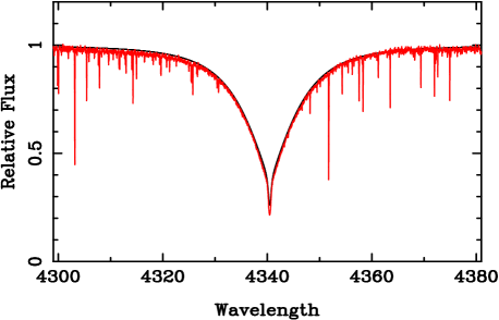
Figure 1: H$\gamma$ profile for $T_{\rm eff}=13100$K, $\log(g)=4.0$. The calculated profile is nearly obscured by the observations (gray, red in online version). The HD 65949 profile is from a HARPS (Mayor et al. 2003) spectrum obtained on 31 March 2009. No metal lines were included in the calculation.

No stratification was assumed in any of the abundance calculations.

4 Spectra

ESO/FEROS spectra are discussed in Kaufer et al. (1999). The useful coverage was $\lambda\lambda$3603-9211, with a resolving power of 48000. They were supplemented by a UVES (Dekker et al. 2000) spectrum obtained on 4 August 2008 ($\lambda\lambda$3258-4517, and 5655-9464). The resolving power in the blue arm is 80000, and 110000 in the red. Additionally, we used HARPS spectra obtained on 14 December 2008, 31 March 2009, 2 June 2009, and 3 June 2009. The wavelength coverage is $\lambda\lambda$3972-6911, with a resolving power of 120000. Most quantitative measurements were made on the December 2008 spectrum, where the signal-to-noise (S/N) was 120 to 150.

Most abundances are based on equivalent width measurements carried out with Michigan software, which fit a Voigt profile to the stellar features. Equivalent widths for few hyperfine and helium profiles were obtained from quadrilaterals or triangles estimated to have the same area as the more complex absorption profiles.

5 Binarity

Table 1: New radial velocity measurements of HD 65949

	HJD$-2400000$	phase	$V_{\rm r}$ (km s-1)	Spectrograph
	50835.6937	0.7901	45.80	REOSC
	50836.6782	0.8363	43.50	REOSC
	53663.8587	0.6686	46.38	FEROS
	53664.7578	0.7109	47.26	FEROS
	53665.7295	0.7565	47.57	FEROS
	53666.7902	0.8064	46.65	FEROS
	53890.4733	0.3159	20.34	REOSC
	53890.4882	0.3166	20.91	REOSC
	53891.4820	0.3633	26.92	REOSC
	53893.4307	0.4549	34.05	EBASIM
	53894.4388	0.5022	38.96	EBASIM
	54462.7415	0.2034	2.10	REOSC
	54682.9258	0.5485	38.32	UVES
	54683.9155	0.5950	40.63	UVES
	54814.8034	0.7446	45.48	HARPS
	54907.6066	0.1049	-13.63	REOSC
	54921.5702	0.7610	45.05	HARPS
	54985.4926	0.7643	44.72	HARPS
	54985.5149	0.7654	44.72	HARPS

HD 65949 was one of the objects investigated in NGC 2516 for binarity by Abt and Levy (1972). Their observations were combined with objective prism measurements by Gieseking (1978) and Gieseking and Karimie (1982), who found orbital elements very close to those adopted here (Table 2). We may group the radial velocities roughly into two time periods. The “old” measurements were made within the interval from Nov. 1967 through Apr. 1978. “New” measurements followed some 20 years later, from Jan. 1998 to the Jun. 2009. The newer measurements are clearly more precise, as shown in Fig. 2. This is expected, as many of the older measurements were made from objective prism spectra.

Table 1 gives the more recent, previously unpublished, radial velocities, plotted in Fig. 2. The ESO FEROS and UVES instruments are discussed in §4. The REOSC spectrograph is described by González and Lapasset (2000); Pintado and Adelman (2003) discuss the EBASIM instrument.

Even though the old measurements are less precise by a factor 10–100, they are useful for the period calculation since they provide a time-base of about four decades. We performed a global fit of all the observations to determine the period. Then we kept the period fixed and fit the remaining parameters using only the new measurements. The resulting parameters are listed in Table 2.

Table 2: SB1 orbital elements and corresponding mass function, $f(m)$, for HD 65949. Elements other than the period use only recent data.

Element	Value	Error
$V_{\gamma}$ (km s-1 )	25.7	$\pm$	1.9
$K_{1}$ (km s-1)	29.5	$\pm$	1.4
$\omega$ (deg)	148	$\pm$	7
$e$	0.40	$\pm$	0.05
$P$ (d)	21.2836	$\pm$	0.0012
$f(m)$ (M⊙)	0.0437	$\pm$	0.0067

Figure 2: Old (dots) plus new (filled circles) radial velocities using orbital elements of Table 2. A closer fit to the new data may be obtained if the period is determined only from the new data. The current plot highlights the $\gamma$-velocity difference between the old and new data.

The adopted $T_{\rm eff}=13100$ K, and a fit to the data of Torres, Andersen, and Giménez (2009) then yields $M_{V}=-0.02$, for a main sequence star. The corresponding mass is $\approx 3.3\,M_{\odot}$. Since no absorption lines from the secondary are seen, we assume a flux ratio $\leq 0.1$, or $\Delta M_{v}>2.5$. The calibration gives $M/M_{\odot}\approx 1.52$, for $M_{V}\approx 2.48$, commensurate with a mass ratio, $q<0.5$, expected for main-sequence binary stars. If we fix the primary mass at 3.3 $M_{\odot}$, the mass function, $f(m)=0.0446$, yields a secondary mass between 1.52 and 0.92 $M_{\odot}$ for inclinations in the range 41 to 90^∘. Smaller inclinations are less likely, since they would lead to larger secondary masses. Masses of 3.3 $M_{\odot}$ for the primary, and from 1.52 to 0.92 $M_{\odot}$ for the secondary give separations $a_{1}+a_{2}$ from 0.254 to 0.243 AU.

The binarity of the HD 65949 system is of interest in view of the suggestion made below that mass exchange may be relevant for the surface chemistry. We note the increase in the systemic velocity of the binary system, which appears convincing in spite of the larger scatter of the older measurements. Note also that there is a systematic difference of 2 $\rm km\,s^{-1}$between the FEROS and HARPS observations, taken at the same phase, but separated by 3.5 years.

A fit of the center-of-mass velocity, keeping all other orbital parameters fixed, gives $V_{\gamma}=16.9\pm 1.5$ km s^-1 and $V_{\gamma}=25.7\pm 0.2$ km s^-1 for the old and the new measurements, respectively. A third body is therefore suspected to account for the change in systemic velocity.

6 Atomic parameters

Most of the atomic lines used in the present study were sufficiently weak that damping parameters are not important. We used default Stark damping from Cowley (1971), and Unsöld’s (1955) formula for van der Waals damping, but enhanced by a factor of two. Only the Ca ii K-line and lines from the infrared triplet were strong enough that Stark damping began to be relevant. We used the parameters adopted by CH04.

Default oscillator strengths were from VALD (Kupka et al. 1999), but supplemented as noted in the element-by-element discussion in Appendix A. Special calculations of partition functions and oscillator strengths were made for the present study, as noted in the Appendices B and C.

For Cr ii, Ti ii, and Mn ii, we used VALD and Kurucz (1995) to retain only lines that were allowed by $LS$-coupling selection rules. All oscillator strengths for third spectra of the lanthanides were from the DREAM database (Biémont, Palmeri, and Quinet 1999).

7 Abundances

Table 3 lists abundances or upper limits for 58 elements listed in Column 1. Logarithmic ratios of individual abundances to the total elemental abundances including hydrogen follow in Column 2. Column 3 gives error estimates, which are usually the standard deviation of the results from the number of lines used, shown in Column 4. For a few elements, the error is the difference in determinations from two ionization stages. There is no entry for upper limits based on a single line, but we estimate an uncertainty of some 0.5 dex. The solar abundance from Asplund, Grevesse, Sauval and Scott (2009) is in Column 5, while Column 6 is the difference in the stellar and solar values.

  El $\log(N/N_{\rm tot})$ $\pm$(sd) n $(\log(N/{N_{\rm tot}})_{\odot}$ [$N$] He $-1.95$ 0.14 8 $-1.11$ $-0.84$: C $-3.67$ 0.40 2 $-3.61$ $-0.06$ N $\leq-6.52$ 1 $-4.21$ $-2.31$: O $-3.24$ 0.16 9 $-3.35$ $0.11$: Ne $-4.29$ 0.16 10 $-4.11$ $-0.18$ Na $-5.42$ 0.13 2 $-5.80$ $0.38$ Mg $-4.80$ 0.45 13 $-4.44$ $-0.36$ Al $-6.44$ 0.24 4 $-5.59$ $-0.85$ Si $-4.69$ 0.26 12 $-4.53$ $-0.16$ P $-5.13$ 0.29 19 $-6.63$ $1.50$ S $-4.92$ 0.24 34 $-4.92$ $0.00$ Cl $\leq-7.09$ 1 $-6.54$ $\leq-0.55$ Ar $\leq-6.07$ 1 $-5.64$ $\leq-0.43$: Ca $-5.81$ 0.53 8 $-5.70$ $-0.11$: Sc $-8.18$ 0.07 $-8.89$ $0.71$ Ti $-6.89$ 0.28 54 $-7.09$ $0.20$ V $\leq-8.65$ 1 $-8.11$ $\leq-0.54$ Cr $-5.87$ 0.31 63 $-6.40$ $0.53$ Mn $-6.06$ 0.15 22 $-6.61$ $0.55$ Fe $-4.06$ 0.24 98 $-4.54$ $0.48$ Co $\leq-5.76$ $-7.05$ $\leq 1.29$ Ni $-6.35$ 0.31 5 $-5.82$ $-0.53$ Cu $\leq-5.81$ 1 $-7.85$ $\leq 2.04$ Zn $\leq-7.8$ 1 $-7.48$ $\leq-0.32$ Ga $\leq-7.50$ 1 $-9.00$ $\leq 1.50$ Br $-6.81$ 0.50 3 $-9.50$ $2.69$ Kr $-5.85$ 0.13 5 $-8.79$ $2.94$ Rb $\leq-6.70$ 1 $-9.52$ $\leq 2.82$ Sr $-6.76$ 0.45 6 $-9.17$ $2.41$ Y $-7.66$ 0.11 14 $-9.83$ $2.17$ Zr $-7.90$ 0.17 3 $-9.46$ $1.56$ Nb $-7.26$ 0.29 22 $-10.58$ $3.32$ Mo $-7.86$ 0.34 4 $-10.16$ $2.30$ Ru $-6.50$ 0.48 20 $-10.29$ $3.79$ Rh $-7.43$ 1 $-11.13$ $3.70$ Pd $-5.84$ 0.14 4 $-10.47$ $4.63$ Cd $\leq-7.82$ 1 $-10.33$ $\leq 2.51$ Sn $\leq-8.42$ 1 $-10.00$ $\leq 1.58$ Xe ${\bf-5.42}$ 0.11 6 $-9.80$ ${\bf 4.38}$ Cs $-7.50$ 1 $-10.96$ $3.46$ Ba $\leq-9.64$ 1 $-9.86$ $0.22$ Ce $\leq-9.79$ 1 $-10.46$ $0.67$ Pr $-8.31$ 0.21 16 $-11.32$ $3.01$ Nd $-8.03$ 0.32 12 $-10.62$ $2.59$ Eu $\leq-8.50$ 1 $-11.52$ $\leq 3.02$ Dy $-8.06$ 0.44 12 $-10.94$ $2.88$ Ho $-8.18$ 0.31 12 $-11.56$ $3.38$ Er $-8.80$ 0.21 3 $-11.12$ $2.32$ Yb $-8.69$ 1 $-11.20$ $2.51$ W $\leq-8.14$ 1 $-11.19$ $\leq 3.05$ Re $-5.81$ 0.27 32 $-11.78$ $5.97$ Os $-5.27$ 0.53 13 $-10.64$ $5.37$ Pt $-5.22$ 0.15 6 $-10.42$ $5.20$ Au $-6.96$ 0.52 3 $-11.12$ $4.16$ Hg $-4.59$ 0.29 4 $-10.87$ $6.28$ Pb $\leq-8.12$ 1 $-10.29$ $\leq 2.17$ Bi $\leq-8.00$ 0.50 2 $-11.39$ $\leq 3.39$ Th $-9.18$ 0.17 8 $-12.02$ $2.84$

Table 3: Abundances in HD 65949, the solar system, and their differences (see text). Results for individual ions may be found in Appendix A.

The stellar abundances are plotted in Fig. 3, along with corresponding solar values. Generally small deviations from the solar pattern are seen, especially for the even-Z elements with Z less than about 30. Beyond this point, the stellar abundances scatter wildly, with excesses ranging up to 6 dex (Re and Hg).

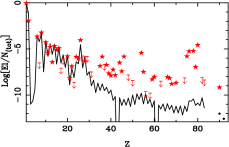
Figure 3: Solar (black line) and stellar (stars) abundances. Upper limits are indicated by horizontal lines with arrows pointing down. Solar points for uranium and thorium are filled circles.

8 Non-nuclear signatures

The abundance pattern of Fig. 3 shows a number of features that indicate the influence of non-nuclear processes. Interestingly, all such indications are for elements with Z greater than about 30 (Zinc). The most common non-nuclear pattern shown in late-B CP stars is an abundance of Mn (Z = 25), greater than that of either Cr (Z = 24) or Fe (Z = 26). This has been called an odd-Z anomaly, since nuclear processes do not make more of odd-Z elements relative their even-Z neighbors (Li, Be, B excepted). That anomaly at Mn is not seen in HD 65949, but does appear in the typical HgMn star HR 7143 (CH04).

Beyond the iron peak, there is often an odd-Z anomaly at yttrium (Z = 39), which can be more abundant than its even-Z neighbors, Sr and Zr (Guthrie 1971, Adelman et al. 2001). This anomaly is clearly present in HR 7143, but not in HD 65949. However, the next triplet containing an odd-Z element, Zr, Nb (Z = 41), Mo does form an odd-Z anomaly in HR 65949. CH04 do not report abundances for Nb and Mo. Indeed, abundances for these two elements are rarely (if ever) reported for HgMn or related (HR 6000, HR 6870) stars.

Just as significant as the odd-Z anomalies are two highly fractionated even-Z neighbors: Xe and Ba. We find Xe more abundant than Ba by 4.2 or more dex. None of the standard (r- or s-process) neutron addition schemes would produce so severe a fractionation. Note that a Xe-Ba fractionation of 3.31 dex occurs in HR 7143. Similar (or larger) values probably hold for other HgMn stars where Xe ii has been identified. However, the Ba ii lines are presumably not seen, and upper limits have not been computed.

9 Late B-star abundances compared

9.1 HD 65949 and HR 7143

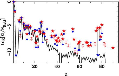
Figure 4: Solar abundances are again given by the solid black line. The stars or upper-limit symbols again indicate abundances for HD 65949. Filled circles show abundances for HR 7143. When elements are determined in both stars, a vertical line connects the two values. Note the enormous difference in the osmium abundances (Z = 76).

Figure 4 is a similar to Fig. 3, but shows abundances of both HD 65949 and HR 7143 (CH04). Vertical lines connect elements with abundances available for both stars. Among the elements below zinc (Z = 30), the even-Z elements, especially the lighter ones, are not far from their solar values. Larger departures from the solar pattern are seen among the odd-Z elements. These are usually small or negative in HD 65949. A nitrogen (Z = 7) deficiency is a general characteristic of HgMn stars (Dworetsky 1993). Phosphorus (Z = 15) is overabundant in both stars, but not more so than its even-Z neighbors. Manganese (Z = 25) is slightly overabundant in HD 65949, but 2.5 dex in excess in HR 7143. Overall, we may conclude that the lighter elements of HR 7143 show a greater fractionation from the solar pattern than those of HD 65949.

When we consider the heavier elements, both stars show a large scatter, nearly exclusively of positive deviations from solar. Gallium is particularly notable, as it is some 3.7 dex overabundant in HR 7143. The upper limit in HD 65949 is about 1.7 dex. There is no indication of the stronger Ga ii lines on the HARPS spectra. Apart from Ga and Y, the excesses in HR 7143 are lower than in HD 65949. Note, especially the case for Os (Z = 76) which is 5.3 dex in excess in HD 65949 but essentially solar in HR 7143.

Generally, among the elements heavier than zinc, the abundances in HD 65949 are more highly fractionated than those of HR 7143.

9.2 $\chi$ Lup

Abundances for $\chi$ Lup A ($T_{\rm eff}=10165$ K, $\log(g)=3.8$, B9.5p HgMn) are given by Leckrone et al. (1999) as supplemented by papers cited by Wahlgren (2005). A plot of abundances vs. Z reveals a relatively small scatter for most elements lighter than those with Z in the early 30’s. This has been noted for HD 65949 and HR 7143. There are, however, several points for elements studied in the $HST$ UV spectra. In particular, the marked underabundance of zinc (Z = 30) is prominent. The triplet Zn, Ga (Z=31), and Ge (Z = 32) form an even-Z anomaly, incomprehensible from the point of view of nucleosynthesis. The same even-Z anomaly is shown by Ga, Ge, and As. No marked overabundances occur in $\chi$ Lup until Z = 33. Beyond that value of Z, overabundances are common, and there are no underabundances for detected elements. Dworetsky, Persaud & Patel (2008) give $\log(Xe/H)=-5.74$, between the values for HR 7143 and HD 65949. There is no abundance for the noble gases Kr (Z=36). Strontium (Z = 38) is enhanced in both HD 65949 and $\chi$ Lup. Barium (Z=56) is significantly enhanced only in $\chi$ Lup and in HgMn stars, but not in HD 65949. Rhenium (Z = 75), so highly enhanced in HD 65949, has no detection in $\chi$ Lup. The overall very heavy element (Os, Pt, Au, Hg, Tl) enhancement in Chi Lup is present, but differs in detail from that of both HD 65949 and HR 7143.

We leave further discussion and possible interpretation of the $\chi$ Lup abundances to a future study.

10 Discussion

10.1 The temperature differential

We reject the temperature differential, some 1100 K, as primarily responsible for the abundance differences discussed in the previous section. That is because similar abundance patterns persist in HgMn stars over comparable temperature ranges. Moreover, strong Hg and especially Pt are more common among cooler HgMn stars than hotter ones, and these elements are more abundant in the hotter star, HD 65949 than the cooler HR 7143. A similar argument applies to the Mn abundance, but with a reversed sense. Here the hotter HgMn stars are generally richer in Mn, but the cooler HR 7143 has the larger Mn abundance excess.

The isotopic composition of Hg in HD 65949, is also more typical of cooler HgMn stars than that of HR 7143. At low resolution, a mean wavelength of the Hg ii feature may indicate an enrichment of the heavier isotopes–generally the cooler HgMn stars have longer center-of-gravity wavelengths for the $\lambda$3984 feature. However, for HR 7143, we measured a mean position of 3983.858 Å  on a 2.4 Å/mm plate taken at the Dominion Astrophysical Observatory (9682/10858u). This might be compared with the FEROS wavelength (cf. Paper I) of 3984.01 Å  for HD 65949. Synthesis of the higher-resolution HARPS and UVES spectra available today prove that HD 65949 is richer in heavier Hg isotopes, though ²⁰⁴Hg does not dominate, as in $\chi$ Lup.

10.2 Nuclear patterns

The elements Sr and Ba are typically associated with the s-process. While the Sr excess is more than 2 dex, Ba is at most marginally enhanced, and could be depleted. This excludes the relevance of that process. On the other hand, the solar system r-process shows excesses at Te and Xe, and again, at Os and Pt. The former peak is associated with the N=82 neutron shell closing, and the latter closed shell at N=126. We have not reported an abundance for Te, but the element is positively identified, and surely in excess. Oscillator strength calculations currently under way will provide a quantitative result.

We have noted that the idea of mass transfer in connection with CP star anomalies is relatively old. Wahlgren et al. (1995) discuss it briefly in connection with the isotopic anomalies in $\chi$ Lup that suggest the r-process. We note also, the shrewd observation of Woolf and Lambert (1999) that the stable, lighter Hg isotopes are never enhanced in HgMn stars, and that these are the only two isotopes not produced by the r-process. On the other hand, Proffitt and Michaud (1989) concluded the likely transferrence of a significant amount of material from a nearby supernova to a B or A star was “one in a few thousand.” Even if HD 65949 represents that rare star, the abundances of the heavy elements are severely fractionated from a pure nuclear pattern. The anomalies cannot result only from an admixture of nuclear-processed material.

We therefore look within this pattern for some clue to the relevant fractionation mechanism. The favored mechanism would be in situ separation by radiative and gravitationally driven diffusion.

10.3 Theoretical predictions

Surprisingly little theoretical work is of relevance to the present task. An exception is the decades-old, but extensive work by Michaud, Charland, Vauclair, & Vauclair (1976, MCVV). In this work both time scales, and extensive predictions are made through the lanthanide elements. In Fig. 6 of MCVV there are precipitous abundance drops near Z = 38-40, and 56-58. This suggests a depletion at Sr, which we do not see, and one at Ba, which we may. On the other hand, the calculations for the heavier elements were sufficiently rough that most elements were predicted to be overabundant by about the same amount. Only when relevant ions achieved the noble gas configurations (e.g. Sr iii or Ba iii) was there a significant reduction of the radiative to gravitational (plus temperature-gradient) forces ($g_{R}/g_{GT}$). That ratio was more or less constant for most of the elements beyond Z = 30, and could not account for the structure seen in our Fig. 3.

The basic diffusion hypothesis has always been that the stars arrive on the main sequence with abundances that are well mixed. Chemical separation then took place as a result of a time-dependent process. Nevertheless, there has been almost no attempt to interpret abundances in terms of age.

The concept of age, as we need it here, need not be a chronological age, or years on the main sequence. MCVV and many subsequent studies (cf. Richer, Michaud, & Turcotte 2000) added a “turbulent” component to the diffusion coefficient. Without this modification much larger anomalies than those observed in some CP stars would be predicted. The more effective this turbulence, the slower the diffusion processes would be. Thus we must think of age in a relative sense. Chemical or cosmochemical maturity might be a more appropriate phrase than age.

For stars with masses above 2-2.6 $M_{\odot}$, MCVV found characteristic diffusion times very short with respect to the stellar lifetimes. They proceeded to predict abundance anomalies for these stars, without consideration of the ages or the length of time since the diffusion began to operate. Presumably, this was because the time scales were found to be very short, after which time an approximate equilibrium abundance pattern might be established.

This basic picture does not account for the occurrence of very different abundances in stars with similar temperatures and surface gravities.

10.4 Correlations

Suppose exotic material from a supernova were transferred to the surface of a nearby star. We must imagine the material to have characteristic r-process enhancements, and minor amounts of elements with Z $<$ 30.

This material could be subject to grain condensation, followed by gas-grain separation as in the scenario proposed by Venn and Lambert (1990) to explain $\lambda$ Boo stars. In our case, the elements that resist grain formation (Xe, Kr, Os, Pt, Hg) would be carried to the star. One might then expect to see a correlation of the abundance excesses with condensation temperatures (e.g. Lodders, 2003). However, we find no significant correlation of this kind.

We therefore favor a second model.

Figure 5 shows that there is a correlation of the abundance excesses of the heavier elements with the second ionization potential. The significance of the correlation is 0.0013. The figure and significance calculation includes two points for Ba and Ce for which we have only upper limits. Should we exclude them, the significance drops to 0.016. However, if we use abundances for these elements decreased by 1 and even 2 dex, the significance of the correlation is essentially the same as with the upper limits: 0.0016.

While it is clear that other factors than the second ionization potential determine the overabundances, the correlation we find is unlikely to have arisen by chance.

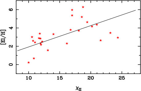
Figure 5: Logarithmic abundance excesses for elements with Z $>$ 30 vs. second ionization energies. Upper limits are not included. The line is a least squares fit. The correlation coefficient, 0.608, is significant at the 0.0013 level for 25 points.

The proposed model supposes that exotic r-processed material fell onto the star, and then was subject to in situ differentiation. One advantage of this model is that it would not require the diffusion of rhenium or mercury from great depths requiring the elements to pass through many ionization stages.

The “mass above the photosphere” may be defined as $\int\rho dx$ from $x=0$ to a physical depth where the optical depth is about unity. For late B stars, that mass is about 0.1  gm cm^-3. This means that to enhance the Hg abundance by a factor of $2\cdot 10^{6}$, ions would have to diffuse upward from a depth such that $\int\rho dx\approx 2\cdot 10^{5}$. We use the 2.5 $M_{\odot}$ model of P. Demarque, D. Guenther, and J. Howard (cf. Cowley 1995, Table 9.3(b)). Numerical integration of the tabulated values show that at this depth ($r/R=0.92$), $T=4\cdot 10^{5}$K. If we use the Saha equation, taking the ratio of the relevant partition functions to be unity, we find the ratio of Hg⁺¹⁶ to Hg⁺¹⁵ approximately unity at this depth ($9.6\cdot 10^{4}$  km below the surface of the star).

This calculation assumed mercury that has diffused upward does not escape from the photosphere. We also have neglected lowering of the ionization energy. Both effects would increase the relevant degree of ionization. The ionization energy for Hg xvi (+15) used here is from Carlson et al. (1970). The value, 357 eV, is approximate, but adequate for the present purposes, which is only to show the multiplicity of ion stages involved. The overall situation is not substantially different from that discussed by Cowley and Day (1976), where it was concluded that for an enhancement of $10^{5}$ mercury would have to diffuse from depths involving Hg xi-xiii, and the relevant temperature (see Table 1. Model B) was $2\cdot 10^{5}$.

Diffusion from deep layers does not provide a basis for understanding the correlation with the second ionization potential.

10.5 Predictions

Based on the model of the preceeding section, and the abundances of HD 65949 and HR 7143 (as typical of HgMn stars), we can make a number of predictions that can be checked by further investigation. The overall hypothesis is that both stars have been subject to exotic mass addition, but that HD 7143 is cosmochemically more mature then HD 65949.

• Osmium and rhenium are rarely (if ever) enhanced to the point where they are identified in ground-based spectra of HgMn stars. Therefore, these elements cannot be (strongly) supported by radiation in the atmospheres of HgMn stars compared, for example, to mercury. (Their high abundance in HR 65949 must result from a very recent transfer of material.)

• Xenon is often found in HgMn stars. In spite of the fact that Xe i has noble gas structure, significant support for this element must exist. The case of Kr needs more observational material. Though it is not seen in HgMn stars, better observations could lead to its identification. We see no indication of Kr ii $\lambda$4355.48 in HR 7143 on CH04 material posted on Castelli’s web site.

• The nitrogen deficiency and the phosphorus excess must be established rapidly in HD 65949. These anomalies appear before a significant Mn excess appears.

• The large gallium abundance shown by many HgMn stars is not seen in HD 65949. Therefore, it must be pushed up from considerable depths, on a time scale longer than relevant for HD 65949. It would be a pure diffusion anomaly.

Of course, it may be possible to account for the abundance pattern of HR 65949 with the fundamental diffusion picture when the necessary atomic data are known. The lack of barium enhancement may already be explained in MCVV. The overall scatter of the heavier elements could be attributed to the relative ease of transport of atoms with initially low abundances. This would mean that mercury and rhenium were pushed up from deep layers where atoms might be ten or more fold ionized. We would then conclude that the observed correlation with second ionization potential was a red herring.

11 Acknowledgements

We thank P. North and B. Smalley for computer codes, and J. R. Fuhr J. Reader, and W. Wiese of NIST for advice on atomic data and processes. Thanks also to J. J. Cowan for comments on the abundance pattern in HD 65949 from the point of view of nucleosynthesis. This research has made use of the SIMBAD database, operated at CDS, Strasbourg, France. Our calculations have made extensive use of the VALD atomic data base (Kupka et al. 1999). Thanks are also due to M. Netopil for help during observations in August of 2008. CRC thanks John Hutchings, Murray Fletcher, and his colleagues at Michigan, especially Ming Jhao, for numerous ideas and comments. Thanks are due to J. Andersen and G. Torres for a preprint of their review paper on the masses and radii of normal stars. Financial support of the Belgian FRS-FNRS is also acknowledged. GMW acknowledges support from NASA grant NNG06GJ29G.

REFERENCES

Abt, H. A., Levy, S. G. 1972, ApJ, 172, 355

Abt, H. A., Morgan, W. W. 1969, AJ, 74, 813

Adelman, S. J., Snow, T. P., Wood, E. L., Ivans, I. I., Sneden, C., Ehrenfreund, P., Foing, B. H. 2001, MNRAS, 328, 1144

Asplund, M., Grevesse, N., Sauval, A. J., Scott, P. 2009, ARA&A. 47, 481

Blaise, J., Wyart, J.-F. 2009, online data tables:
http://www.lac.u-psud.fr/Database/Contents.html

Biémont, E., Grevesse, N., Kwiatowski, M., Zimmerman, P. 1982, A&A, 108, 127

Biémont, E. Palmeri, P., Quinet, P. 1999, Astrophys. Sp. Sci., 269-270, 635. See also the online data base: (http://w3.umh.ac.be/$\sim$astro/dream.shtml)

Carlson, T. A., Nestor, C. W. Jr., Wasserman, N. McDowell, J. D. 1970, Atomic Data, 2, 63

Castelli, F. 2009, wwwuser.oats.ts.astro.it/castelli/

Castelli, F., Hubrig, S. 2004, A&A, 425, 263 (CH04)

Cowan, R. D. 1981, The Theory of Atomic Structure and Spectra (Berkeley, CA: Univ. Calif. Press)

Cowley, C. R. 1971, Obs., 91, 139

Cowley, C. R. 1995, An Introduction to Cosmochemistry, (Cambridge: University Press)

Cowley, C. R., Barisciano, L. P., Jr. 1994, Obs., 114, 308

Cowley, C. R., Day, C. A. 1976, ApJ, 205, 440

Cowley, C. R., Wahlgren, G. M. 2006, A&A, 447, 681

Cowley, C. R., Hubrig, S., Wahlgren, G. M. 2008, J. Phys. Conf. Ser., 130, 12005 (Paper II)

Cowley, C. R., Hubrig, S., González, G. F., Nuñez, N. 2006, A&A, 455, L21 (Paper I)

Dekker, H., et al. 2000, SPIE, 4008, 534

Dolk, L., Litzén, U., Wahlgren, G. M. 2002, A&A, 388, 692

Dworetsky, M. M. 1993, in Peculiar Versus Normal Phenomena In A-Type And Related Stars, ed. M. M. Dworetsky, F. Castelli, and R. Faraggiana, ASP Conf. Ser., 44, 1

Dworetsky, M. M., Storey, P. J., Jacobs, J. M. 1984, Phys. Scr. T8, 39

Dworetsky, M. M., Persaud, J. L., Patel, K. 2008, MNRAS, 385, 1523

Engleman, R. 1989, ApJ, 340, 1140

Fivet, V., Quinet, P., Biémont, É., Xu, H. L. 2007, J. Electron. Spec. Relat. Phen., 156-158, 250

Fuhr J. R., Wiese, W. L. 1996, NIST Atomic Transition Probability Tables, CRC Handbook of Chemistry & Physics, 77th Edition, ed. D. R. Lide, CRC Press, Inc., Boca Raton, FL

Fuhr, J. R., Wiese, W. 2006, J. Phys. Chem. Ref. Data, 35, 1669

Gieseking, F. 1978, A&AS, 32, 17

Gieseking, F., Karimie, M. T. 1982, A&AS, 49, 497

González, J. F., Lapasset, E. 2000, AJ, 119, 2296

Grevesse, N. 2008, in Comm. in Astroseismology, Vol. 157, 156 (Wrocklaw HELAS Workshop), ed. M. Breger, W. Dziembowski, & M. Thompson.

Guthrie, B. N. G. 1971, Astrophys. Sp. Sci., 10, 156

Hauck, B., Mermilliod, M. 1998, A&AS, 129, 431

Hubrig, S., North, P., Schöller, M., Mathys, G. 2006, AN, 327, 289

Ivarsson, S., Wahlgren, G. M., Dai, Z., Lundberg, H., Leckrone, D. S. 2004, A&A, 425, 353

Kaufer, A., Stahl, O., Tubbesing, S., Nørregaard, P., Avila, G., Francois, P., Pasquini, L., Pizzella, A. 1999, ESO Messenger, 95, 8

Klinkenberg, P.F.A., Meggers, W.F., Velasco, R., Catalan, M.A. 1957, J. Res. Natl. Bur. Stand., 59, 319

Kramida, A. E., Shirai, T. 2006, J. Phys. Chem. Ref. Data, 35, 423

Kunzli, M., North, P., Kurucz, R. L., Nicolet, B. 1997, A&AS, 122, 51

Kupka, F., Piskunov, N. E., Ryabchikova, T. A., Stempels, H. C., Weiss, W. W. 1999, A&AS, 138, 119

Kurucz, R. L. 1993, CD-ROM No. 18 (Smithsonian Ap. Obs.)

Kurucz, R. L. 1995, CD-ROM No. 23 (Smithsonian Ap. Obs.)

Leckrone, D. S., Proffitt, C. R., Wahlgren, G. M. Johansson, S. G., Brage, T. 1999, AJ., 117, 1454

Ljung, G., Nilsson, H., Asplund, M., Johansson, S. 2006, A&A, 456, 1181

Lodders, K. 2003, ApJ, 591, 1220

Mayor, M., Pepe, F., Queloz, D., et al. 2003, ESO Messenger, 114, 20

Meggers, W. F., Catalan, M. A., Sales, M. 1958, J. Res. Natl. Bur. Stand., 61, 441

Meggers, W. F., Corliss, C. H., Scribner, B. F. 1975, NBS Monog. 145

Meléndez, J., Barbuy, B. 2009, A&A, 497, 611

Mermilliod, J.-C., Hauck, B., Mermilliod, M. 2007, General Catalogue of Photometric Data, http://www.unige.ch/siences/astro/

Michaud, G. 1970, ApJ, 160, 641

Michaud, G., Charland, Y., Vauclair, S., Vauclair, G. 1976, ApJ, 210, 447 (MCVV)

Moon, T. T. 1984, Comm. Univ. London Obs., No. 78

Moon, T. T., Dworetsky, M. M. 1985, MNRAS, 217, 305

Moore, C. E. 1949-1958, Atomic Energy Levels, Vols. I-III, NBS Circ. 467 (Washington, D. C.: US Gov. Print. Off.)

Munari, U., Zwitter, T. 1997, A&A, 318, 269

Nilsson, H., Ivarsson, S. 2008, A&A, 492, 609

Nilsson, H., Ljung, G., Lundberg, H., Nielsen, K. E. 2006, A&A, 445, 1165

Palmeri, P., Quinet, P., Biémont, É., Svanberg, S., Xu, H.L. 2006, Phys. Scr., 74, 297

Palmeri, P., Quinet, P., Biémont, É., Xu, H.L., Svanberg, S. 2005, MNRAS, 362, 1348

Palmeri, P., Quinet, P., Fivet, V., Biémont, É., Cowley, C. R., Engström, L., Lundberg, H., Hartman, H, Nilsson, H. 2009, J. Phys B 42, 165005

Paunzen, E., Schnell, A., Maitzen, H. M. 2006, A&A, 458, 293

Pickering, J. C., Thorne, A. P., Perez, R. 2001, ApJS, 132, 403 (Erratum: ApJS, 138, 247, 2002)

Pintado, O. I., Adelman, S. J. 2003, A&A, 406, 987

Preston, G. W. 1974, ARA&A, 12, 257

Proffitt, C. R., Michaud, G. 1989, ApJ, 345, 998

Quinet, P., 2002, J. Phys. B., 35, 19

Quinet, P., Palmeri, P., Biémont, É., Jorissen, A., Van Eck, S., Svanberg, S., Xu, H.L., Plez, B. 2006, A&A, 448, 1207

Quinet, P., Palmeri, P., Fivet, V., Biémont, É., Nilsson, H., Engström, L, Lundberg, H. 2008, Phys. Rev. A., 77, 022501

Ralchenko, Yu., Kramida, A.E., Reader, J. and NIST ASD Team 2008, NIST Atomic Spectra Database (version 3.1.5), [Online]. Available: http://physics.nist.gov/asd3 [2010, Jan 24]. National Institute of Standards and Technology, Gaithersburg, MD.

Reader, J., Corliss, C. H. 1980, NSRDS-NBS Monog. 68.

Richer, J., Michaud, G., Turcotte, S. 2000, ApJ, 529, 338

Rosberg, M., Wyart, J.-F. 1997, Phys. Scr., 55, 690.

Ryabtsev, A.N. 2009, (private communication)

Ryabchikova, T., Ryabtsev, A., Kochukhov, O., Bagnulo, S. 2006, A&A, 456, 329

Sansonetti, C. J., Reader, J. 2001, Phys. Scr., 63, 219

Smirnov, Yu. M., Shapochkin, M. B. 1979, Opt. Spectroc., 47, 243

Torres, G., Andersen, J., Giménez, 2010, A&A Rev., 18, 67

Unsöld, A., 1955, Physik der Sternatmosphären, Zweite Aufl. (Berlin: Springer)

van Leeuwen, F. 2009, A&A, 497, 209

Venn, K. A., Lambert, D. L. 1990, ApJ, 363, 234

Wahlgren, G. M. 2005, in The A-Star Puzzle, ed. J. Zverko, J. Žižňovský, S. J. Adelman, W. W. Weiss (Cambridge: Cambridge Univ. Press.), p. 291

Wahlgren, G. M., Johansson, S., Litzén, U., Gibson, N. D., Cooper, J. C., Lawler, J. E., Leckrone, D., Engleman, R. Jr. 1997, ApJ, 475, 380

Wahlgren, G. M., Leckrone, D. S., Johansson, S. G., Rosberg, M., Brage, T. 1995, ApJ, 444, 438

Wolk, S. J., Harnden, F. R. Jr., Murray, S. S., et. al. 2004, ApJ, 606, 466

Woolf, V., Lambert, D. L. 1999, ApJ, 521, 414

Wyart, J.-F. 1977, Optica Pura y Aplicada 10, 177

Zielińska, S., Bratasz, Ł., Dzierżȩga, K. 2002, Phys. Scr., 66, 454

Appendix A Discussion of individual abundances

The Michigan software used to obtain abundances from individual lines is set up to read a data base that is basically VALD, but with numerous additions and edits. For example, for the third spectra of the lanthanides, all values are from the DREAM site. Use of data from original sources often requires line-by-line editing. To avoid this in many cases, we used our default data base, but checked against more recent sources, or against the posting on the NIST site, and if the differences were minor, we did not recompute an abundance.

All averages are logarithmic, that is, the logarithms of abundances for individual lines were averaged directly.

Original sources of oscillator strengths are cited where practicable, but we relied heavily on the online data bases of Ralchenko, et al. (2008, NIST), Kupka, et al. (1999, VALD), and Biémont, Palmeri & Quinet (1999, DREAM). When no source of oscillator strength is explicitly cited, the values come from VALD.

In the following sections, a measured stellar wavelength is indicated by an asterisk, e.g. $\lambda^{*}$4911.66.

Helium (Z = 2; $\log(He/N_{\rm tot})\approx-1.95\pm 0.14$): A rough estimate, using Voigt profiles of 8 He i lines. The helium abundance is about 10 per cent that of the sun.

Carbon (Z = 6; $\log(C/N_{\rm tot})=-3.66\pm 0.4$:): The abundance is from a synthesis of the C ii $\lambda$4267 doublet, which is clearly present. The VALD oscillator strengths are very close to those on the NIST site. A few C i and ii lines are surely present, but give inconsistent abundances, most likely due to blends. The carbon abundance is nearly solar. CH04 find a ca. 0.5 dex deficiency of carbon.

Nitrogen (Z = 7; $\log(N/N_{\rm tot})\leq-6.52$): Neither N i nor N ii can be positively identified. An upper limit of 0.3 mÅ  for N ii $\lambda$8680 gives $\log(N/N_{\rm tot})=-6.52$, corresponding to a deficiency of about 2.4 dex with respect to the sun. CH04 got an upper limit corresponding to a deficiency of $-$1.7 dex in HR 7143.

Oxygen (Z = 8; $\log(O/N_{\rm tot})=-3.24\pm 0.16$): Nine O i lines, excluding the strong triplet $\lambda\lambda$7772, 7774, and 7775 yield a small oxygen excess above to the solar value. Oscillator strengths are from VALD but agree well with NIST. CH04 also find a slight excess of oxygen for HR 7143.

Neon (Z = 10; $\log(Ne/N_{\rm tot})=-4.29\pm 0.16$): A close examination of the HARPS spectra show that Ne I is clearly present. The abundance is based on 10 weak lines and oscillator strengths from NIST. The line-to-line agreement is excellent.

Sodium (Z = 11; $\log(Na/N_{\rm tot})=-5.42\pm 0.13$): The abundance is from the D-lines, with equivalent widths of 27 and 21 mÅ. The probable error is the difference of the two determinations. The stellar lines are much weaker than the interstellar ones.

Magnesium (Z = 12; $\log(Mg/N_{\rm tot})=-4.80\pm 0.45$): The adopted abundance is primarily from 9 Mg ii lines, which give $-4.91\pm 0.17$. We did not use the $\lambda$4481 doublet for an abundance. Four Mg i lines, including the b-lines give $-4.46\pm 0.47$, which might indicate stratification or too hot a model. They are weighted 1/3 in the adopted value. The adopted error is the difference in the Mg I and Mg ii values. Oscillator strengths are from VALD, but are very close to those at the NIST site.

Aluminum (Z = 13; $\log(Al/N_{\rm tot})=-6.45\pm 0.24$): The two strongest Al ii lines, $\lambda\lambda$4663.05 and 6243.36 were measured and so identified in the online wavelength list: http:
www.astro.lsa.umich.edu/$\sim$cowley/hd65949/
A 5.8 mÅ  line is present at the position of the strong Al I line $\lambda$3691.52. This is almost certainly the line 3691.49 on the online list. There is no definite feature at the position of the other strong Al i line, $\lambda$3944.01. However, the noise might obscure a 1 mÅ  feature. We adopt a straight average of two Al i and two Al ii lines. Oscillator strengths were from VALD, but are very close to NIST. Aluminum is deficient. This result was also found by CH05.

Silicon (Z = 14; $\log(Si/N_{\rm tot})=-4.69\pm 0.26$): The abundance is from 10 Si ii and 2 Si iii lines with equivalent widths ranging from 4.6 to 136 mÅ. Oscillator strengths are mostly from NLTELINES (Kurucz 1993). Generally, the agreement with NIST was good. However for $\lambda\lambda$5669 and 5957, we substituted the NIST values, which had B+ accuracy.

The 2 Si iii lines, $\lambda\lambda$4552 and 4567 yield abundances of $-$4.29 and $-$4.46, in fair agreement with the overall mean. Both lines have NIST graded B+ accuracies.

Phosphorus (Z = 15; $\log(P/N_{\rm tot})=-5.13\pm 0.29$): The abundance is based on 19 weak P ii lines. Oscillator strengths are from BELLLIGHT (Kurucz 1993), a compilation from various sources. The overabundance, some 1.6 dex, is substantially above that found by CH04 for HR 7143.

Sulfur (Z = 16; $\log(S/N_{\rm tot})=-4.92\pm 0.24$): The abundance is based on 34 S ii lines with equivalent widths from 1.3 to 17 mÅ. Two outliers, $\lambda\lambda$4162 and 4174 were excluded from the average. The abundance is solar, within the uncertainties. CH04 find sulfur underabundant by 0.4 dex in HR 7143.

Chlorine (Z = 17; $\log(Cl/N_{\rm tot})\leq-7.09$): An upper limit is derived from Cl ii $\lambda$4794.55, which is $\leq 0.3$ mÅ. The oscillator strength is from Fuhr and Wiese (1996).

Argon (Z = 18; $\log(Ar/N_{\rm tot})\leq-6.07$): An upper limit is derived from the strong Ar i line $\lambda$8115.31. The oscillator strength is from Fuhr and Wiese (1996).

Calcium (Z = 20; $\log(Ca/N_{\rm tot})=-5.81\pm 0.53$): The strongest Ca i line, $\lambda$4227 is probably present. We measured a 1.6 mÅ  line just above the noise level. There were seven unblended Ca ii lines. With a microturbulence, $\xi_{t}=1$ $\rm km\,s^{-1}$, the K-line and $\lambda\lambda$8498 and 8542 of the infrared triplet yield an abundance ca. 1 dex higher than the weaker lines, $\lambda\lambda$3706, 8201, 8248, and 8912. The plot of abundance vs. equivalent width looks like a classic case of too low a microturbulence. The adopted mean is the average of assuming $\xi_{t}=1$ and $\xi_{t}=5$ $\rm km\,s^{-1}$. The latter brings strong and weak Ca ii lines into agreement. The uncertainty is the difference in these abundances. We do not consider $\xi_{t}=5$ $\rm km\,s^{-1}$realistic. Interestingly, the strong Ca ii lines agree with the very weak Ca I $\lambda$4227 line. Calcium is poorly determined; the source of the large uncertainty is not understood. The usual culprits are non-LTE or stratification. They are not explored here. Note that the Ca ii K-line and the two components of the infrared triplet are the strongest lines used in the present analysis.

Scandium (Z = 21; $\log(Sc/N_{\rm tot})=-8.18\pm 0.07$): The abundance is based on 5 Sc ii lines, including $\lambda$4246 with equivalent widths from 5.1 to 16.8 mÅ. The internal agreement is good; the standard deviation for the five lines is less than 0.1 dex.

Titanium (Z = 22; $\log(Ti/{N_{\rm tot}})=-6.90\pm 0.27$): Only Ti ii lines are available. The abundance is based on 42 lines with equivalent widths ranging from 2 to 45 mÅ. Oscillator strengths are from Pickering, Thorne, & Perez (2001, PTP). Results were very similar if lines with LS-allowed transitions from Kurucz (1995, used by VALD) were used. No significant trends of abundances with wavelength, equivalent width, or excitation potential were noticed. Three obvious outliers were excluded. If they are averaged in, the abundance would be $-$6.78.

Vanadium (Z = 23; $\log(V/N_{\rm tot})\leq-8.65$): While V ii lines are prominent in the spectra of cooler Am and superficially normal A-stars; the lines are typically weak or absent in hotter CP types. We estimate an upper limit taking the equivalent width of V ii $\lambda$3545.19 to be $\leq 0.5$ mÅ. This is close to the upper limit found for vanadium by CH04.

Chromium (Z = 24; $\log(Cr/N_{\rm tot})=-5.87\pm 0.31$): There is an $\approx$ 1 mÅ  feature at the proper position to be $\lambda$4254.35, the strongest Cr i line in the region. That line alone gives an abundance of $\log(Cr/N_{\rm tot})=-5.6$ in satisfactory agreement with the overall mean of the Cr ii lines. The abundance is based on 64 $LS$-permitted transitions. Only 14 of the 64 lines used were found in the online material published by Nilsson, et al. (2006). A comparison of the LS-permitted lines in VALD and Nilsson et al. (2006) gave a mean of +0.045 for $\log(gf_{\rm VALD})-\log(gf_{\rm Nilsson})$, with a standard deviation of 0.16 dex. This difference was considered negligible at the present level of accuracy. There is a slight trend of abundance with equivalent width that can be removed by assuming $\xi_{t}=3$$\rm km\,s^{-1}$. The resulting average abundance would be $-5.98\pm 0.26$. Since Cr has an even Z, and hyperfine broadening is not anticipated, we retained the result with $\xi_{t}=1$ for consistency with other spectra.

Manganese (Z = 22; $\log(Mn/N_{\rm tot})=-6.06\pm 0.15$): There is no indication of Mn I. The abundance is based on 22 Mn ii lines with strengths ranging from 3.1 to 86 mÅ. There was no trend of abundance with equivalent width with $\xi_{t}=2.0$ $\rm km\,s^{-1}$. Abundances using 1.0 and 3.0 $\rm km\,s^{-1}$  showed slight trends. Only $LS$-allowed transitions were used. We eliminated three outliers after noting their transitions were not LS-allowed, but which had not been caught by our filter.

Iron (Z = 26; $\log(Fe/N_{\rm tot})=-4.06\pm 0.24$): The adopted abundance is from 98 Fe ii lines. Seven Fe iii lines give $-4.09$, while 21 Fe i lines give $-3.72\pm 0.37$. In view of possible stratification we do not consider these values. However, with the cooler model used in Paper II, we obtained $-3.96$, in better agreement with Fe ii and Fe iii, as detailed in Paper II. Oscillator strengths for the first two spectra were from Fuhr and Wiese (1996). For Fe ii, the recent values of Meléndez and Barbuy (2009) made only a 0.01 dex in the average abundance from Fe ii using transitions from Fuhr and Wiese (2006). The iron abundance is about a factor of three above the solar value.

Cobalt (Z = 27; $\log(Co/N_{\rm tot})\leq-5.76$): Neither Co i nor Co ii is firmly identified. An approximate upper limit is set by the absence of the strong Co i line $\lambda$3443.64. If the equivalent width were 0.5 mÅ, the abundance of Co would be $-$5.76. The strong Co ii line $\lambda$4062.73 gives an upper limit $-$5.33, assuming 0.8 mÅ.

Nickel (Z = 28; $\log(Ni/N_{\rm tot})=-6.35\pm 0.31$): The presence of Ni i cannot be confirmed. While a definite line (7 mÅ) is present within 0.01 Å  of the resonance line in Multiplet 19, the next strongest line in that multiplet is absent, as are the next strongest four Ni i lines in Meggers, Corliss, and Scribner (1975). Ni ii is surely present, although weak. The abundance is based on 5 lines with measured equivalent widths from 4.3 to 10 mÅ.

Copper (Z = 29; $\log(Cu/N_{\rm tot})\leq-5.81$): An upper limit was set from Cu i $\lambda$5153.24, and equivalent width possibly $2$ mÅ. An examination of the region of the strongest expected lines did not confirm the identification.

Zinc (Z = 30; $\log(Zn/N_{\rm tot})\leq-7.8$: We can only set an upper limit that is roughly solar. An $\approx 5$ mA line measured at $\lambda^{*}$4911.66 near the position of Zn II $\lambda$4911.63 may be entirely due to a Nd III line tabulated by Ryabchikova, Ryabtsev, Kochukhov, and Bagnulo (2006). If any Zn II feature is present, it is at the level of the noise.

Ga through Selenium (Z = 31$-$34): Neither the first nor the second spectrum of any of these elements can be confirmed to be present. We report an upper limit for gallium of $-7.50$, based on an equivalent width of $\lambda$4251.14 of 0.4 mÅ.

Bromine (Z = 35; $\log(Br/N_{\rm tot})=-6.81\pm 0.5$: The wavelength agreement was very good on two HARPS spectra for the three lines with oscillator strengths on the NIST web site. Equivalent widths for Br ii $\lambda\lambda$4704.9, 4785.5, and 4816.7 of 4.1, 2.4, and 0.4 mÅ  yield $\log(Br/N_{\rm tot})$ of $-$6.64, $-$6.69, and $-$7.39. We use weight 1/2 for the weakest line. The error is an estimate. Br ii is rarely observed in late B stars, but two of these lines were used by CH04, and all three were observed in 3 Cen A (Cowley & Wahlgren 2006). Br ii is judged weakly present in HD 65949.

Krypton (Z = 36; $\log(Kr/N_{\rm tot})=-5.85\pm 0.13$): Five weak Kr ii lines on HARPS spectra have good wavelength agreement with their laboratory values; the derived abundances are all within a factor of two of one another. The spectrum is weak, but present beyond doubt. There are no Kr ii lines in the VALD or Kurucz data bases. We used transition probabilities from the NIST site.

Rubidium (Z = 37; $\log(Ru/N_{\rm tot})\leq-6.70$): A search for the strongest NIST lines in the region observed did yield some possible features for Rb ii. The upper limit is based on an equivalent width of 1.2 mÅ  for Rb ii $\lambda$4244.40, measured at 4244.41 on a HARPS spectrum. The oscillator strength is from Smirnov and Shapochkin (1979).

Strontium (Z = 38; $\log(Sr/N_{\rm tot})=-6.76\pm 0.45$): The Sr ii resonance lines are unmistakable, and give abundances ranging from -6.6 to -6.2, depending on the method of analysis (synthesis vs. equivalent width). We consider these lines to be affected by NLTE or stratification. The abundance is quite uncertain. We take it from the subordinate lines, $\lambda\lambda$4161 and 4305. Two very weak lines $\lambda\lambda$4312.77 and 4414.84 yield significantly higher abundances. We reject them as probably due to severe blending. The oscillator strangths are from VALD, but are not significantly different from NIST.

Yttrium (Z = 39; $\log(Y/N_{\rm tot})=-7.66\pm 0.11$): The abundance is based on 14 Y ii lines from 3327 to 5662 Å. with equivalent widths from 1.3 to 18.4 mÅ. Oscillator strengths are from VALD. Lines in common agree with Fuhr and Wiese (1996).

Zirconium (Z = 40; $\log(Zr/N_{\rm tot})=-7.90\pm 0.17$): Our rough estimate is based on three Zr ii lines with equivalent widths of 5.0, 9.4, and 9.6 mÅ. Oscillator strengths from VALD but for these lines agree sufficiently with Ljung, et al. (2006)

Niobium (Z = 41; $\log(Nb/N_{\rm tot})=-7.26\pm 0.29$): The abundance is based on 22 lines with equivalent widths from 1.6 to 20 mÅ. The transition probabilities were mostly taken from Nilsson and Ivarson (2008). Values for $\lambda\lambda$3517 and 4119 are from VALD. Nb ii is not routinely identified in CP stars; CH04 do not report an abundance for niobium in HR 7143. Niobium creates an odd-Z anomaly, being more abundant than its adjacent even-Z neighbors.

Molybdenum (Z = 42; $\log(Mo/N_{\rm tot})=-7.86\pm 0.34$): The entry in Table 3 is based on four quite weak Mo II lines, with one outlier weighted 1/2. Oscillator strengths are from Quinet (2002).

Ruthenium (Z = 44; $\log(Ru/N_{\rm tot})=6.50\pm 0.48$): The abundance is based on 20 Ru ii lines with equivalent widths ranging from 0.3 to 22 mÅ. We used new oscillator strengths and partition functions recently calculated by the Mons group (Palmeri, et al. 2009).

Rhodium (Z = 45; $\log(Rh/N_{\rm tot})\approx-7.43$): The abundance is based on only one strong Rh ii line in Multiplet 5: $\lambda$3307.37. The (guessed) oscillator strength, $\log(gf)=0.00$ is from Kurucz (1993). CH05 attribted seven features to Rh ii. Five of these lines are below the UV cutoff of our spectra.

Palladium (Z = 46; $\log(Pd/N_{\rm tot}=-5.84\pm 0.14$): The result is based on four weak Pd ilines, and one blended feature. The abundances from the four lines are within a factor of two of one another. Oscillator strengths are from Biémont, Grevesse, and Kwiatowski (1982).
Silver through Tellurium: (Z = 47–52)

• There is no support for Ag i or ii, either from searches for the strongest lines within our wavelength coverage.

• We find only marginal evidence for Cd. The upper limit is from Cd ii 4415.8, possibly present as as a 1 mÅasymmetry to the violet of a stronger, unidentified line, probably Re ii.

• A search for the strongest lines yields no support for the presence Sb ii.

• We derive an upper limit of $\log(Sn/N_{\rm tot})\approx-8.42$ by assuming Sn ii $\lambda$6453.5 has an equivalent width of 1 mÅ. The oscillator strength used was from NIST.

• Tellurium: Te ii is surely present. Oscillator strengths are currently being calculated, and will be reported in due course.

Xenon (Z = 54; $\log(Xe/N_{\rm tot})=-5.42\pm 0.11$): The abundance is based on six Xe ii lines with equivalent widths from 5 to 27 mÅ. Transition probabilities are from Zielińska, Bratasz & Dzierżȩga, K. (2002). The wavelength agreement is excellent. The spectrum is securely identified.

Cesium (Z = 55; $\log(Cs/N_{\rm tot})\leq-7.7$): A single, weak feature centered at $\lambda^{*}$4603.78 provides an upper limit to the Cs abundance. The stellar feature is not broad enough to fit the laboratory hfs (Sansonetti and Andrew 1986), though a partial contribution from Cs II cannot be excluded. The upper limit falls between the abundance of xenon, and an upper limit for barium.

Barium (Z = 56; $\log(Ba/N_{\rm tot})\leq-9.64$): The Ba ii resonance line $\lambda$4554 has an equivalent width no larger than about 0.6 mÅ. There is no indication of the presence of the second component of the doublet, $\lambda$4934.

Cerium (Z = 58; $\log(Ce/N_{\rm tot}\leq-9.79$): The upper limit is based on the non appearance of the strong Ce iii line $\lambda$3454.39, for which we estimate from raw UVES scans that the equivalent width cannot be larger than about 0.1 mÅ. Because of the wavelength placement and intensity distribution of Ce iii, it is more rarely identified in CP stars. The oscillator strength used for $\lambda$3454 was from the DREAM site.

Praseodymium (Z = 59; $\log(Pr/N_{\rm tot})=-8.31\pm 0.21$): The abundance is based on 16 Pr iii lines from 4 to 20 mÅ. The oscillator strengths are from the DREAM site and line-to-line agreement is good ($\pm 0.21$ sd). The strongest likely Pr ii lines are blended. An equivalent width of 0.5 mÅ  for $\lambda$4225 yields an upper limit of $-$7.9 for $\log(Pr/N_{\rm tot})$, which does not seem particularly useful, since Pr iii gives a smaller value, and the general trend is for the third spectrum of the lanthanides to give a higher abundance.

Neodymium (Z = 60; $\log(Nd/N_{\rm tot})=-7.03\pm 0.32$): The abundance is based on 12 Nd iii lines. Five lines had equivalent widths over 20 mÅ, and another three were over 10 mÅ. Oscillator strengths are from DREAM.

Europium (Z = 63; $\log(Eu/N_{\rm tot})\leq-8.50:$): The upper limit is based on Eu III $\lambda$6666.37 (Ryabchikova, et al. 1999). The oscillator strength is from Wyart, et al. (2008). There is no sign of a feature on the HARPS spectrum. A value of 0.4 mÅ  was used to set the upper limit.

Dysprosium (Z = 66; $\log(Dy/N_{\rm tot}=-8.06\pm 0.44$): The abundance is based on 12 Dy iii lines. All had equivalent widths $\leq$ 17 mÅ. Two lines gave abundances about 1 dex higher than the mean of all 12 lines. They were averaged in, but with weight 1/2. Since the logs were averaged, the difference between weighting or not weighting was only 0.1 dex. Oscillator strengths are from DREAM.

Holmium (Z = 67; $\log(Ho/N_{\rm tot})=-8.18\pm 0.31$): The abundance is based on 12 weak Ho iii lines. Ten of the lines used were under 10 mÅ. Oscillator strengths are from DREAM.

Erbium (Z = 68; $\log(Er/N_{\rm tot})=-8.80\pm 0.21$): The abundance is from three Er ii lines, with equivalent widths between 1.4 and 3.3 mÅ. These three are the strongest lines by far in the Reader and Corliss (1980) tabulation. Oscillator strengths are from DREAM.

Ytterbium ($\log(Yb/N_{\rm tot})\approx-8.69$): The result is from Yb iii $\lambda$4028.14, $W_{\lambda}=0.7$ mÅ. Yb ii, $\lambda$4180.81 is possibly present. $W_{\lambda}=0.3$ mÅ, yields $-$9.13. CH04 observed both Yb ii and Yb iii, and obtained an abundance from Yb iii 0.8 dex higher than from Yb ii. This is qualitatively similar to our result.

Tungsten (Z = 74; $\log(W/N_{\rm tot})\leq-8.14$): We cannot establish the presence of W i or W ii. The W ii line in Multiplet 1, $\lambda$3641.42 if present is a weak feature in the wing of Ti ii $\lambda$3641.33. We estimate the equivalent width must be $\leq$ 0.5 mÅ. This gives an upper limit some 2.6 dex above the solar value. The oscillator strength used for $\lambda$3641 from VALD is 0.15 dex larger than that of Kramida and Shirai (2006).

Rhenium (Z = 75; $\log(Re/N_{\rm tot})=-5.81\pm 0.27$): The Re ii spectrum is exceptionally well developed in HD 65949, even though the strongest atomic lines of Re ii are well below our wavelength coverage. Some 120 lines are attributed wholly or partially to Re ii. New oscillator strengths enable us to determine abundances from lines on either side of the Balmer jump (BJ). Using 15 lines to the violet of the BJ, we find $-5.62\pm 0.21$; 17 lines to the red of the BJ give $-5.97\pm 0.22$. The sense of the difference is that the abundance of rhenium is higher in the higher atmosphere. A microturbulence of 4 $\rm km\,s^{-1}$was necessary to remove dependence of abundance with equivalent width. This is reasonably attributed to hyperfine structure which is readily visible on the HARPS spectra. Even so, we omitted two lines with equivalent widths of 116 and 123 mÅ. The overall rhenium excess, is 6 dex, greater than that of any element apart from mercury.

New oscillator strengths and partition functions were calculated by the Mons group. The results are presented in Appendix B1 and C1.

Osmium (Z = 76; $\log(Os/N_{\rm tot})=-5.27\pm 0.53$): Os ii is present beyond any doubt. One can see on the high-resolution HARPS spectra that the lines of Os ii (and Pt ii) are noticably sharper than lines from lighter ions. The abundance is based on 17 lines with equivalent widths ranging from 5 to 38 mÅ. The oscillator strengths are taken from the database DESIRE, and the partition functions are given in Appendix B1.

Platinum (Z = 78; $\log(Pt/N_{\rm tot})=-5.22\pm 0.15$): With Engleman’s (1989) list, we identified 23 lines with Pt ii. There is good evidence that the dominant isotope is ¹⁹⁸Pt (Paper I). We found no credible evidence for Pt I.

We adopt the absolute oscillator strength scale of Quinet, et al. (2008, QPFB). Only three of their lines are available in HD 65949 (3535.89, 3551.36, and 4046.45 Å). Dworetsky, Story, and Jacobs (1984, DSJ) provide oscillator strengths for an additional six lines, but with a different absolute scale. The DSJ scale was based on calculated transition probabilities for ultraviolet lines that were used to fix the stellar abundance of platinum in $\chi$ Lup. Though DSJ give oscillator strengths for four lines (see their Table II), in practice only two ($\lambda\lambda$1777.0 and 2144.0) were used for the abundance which sets the astrophysical scale of DSJ’s Table IV. Additionally $\lambda$4046 is in DSJ’s Table IV and QPFB. If we compare all four of the common UV lines, we find the DSJ $\log(gf)^{\prime}s$ are larger by 0.30. If we compare only the two lines used for abundance, the corresponding figure is 0.22; the DSJ $\log(gf)$ for $\lambda$4046 is 0.42 larger than that of QPFB. We have scaled down all DJS values by 0.30 dex. The adopted abundance is based on eight lines, not including $\lambda$4046, which is blended with Hg I and sensitive to microturbulence and isotope shifts (Engleman 1989). Using plausible assumptions for the microturbulence, and isotope ratios, we can get good agreement from $\lambda$4046 with results from the other Pt II lines. However, a definitive study of isotopes is postponed to a future study.

Gold (Z = 79; $\log(Au/N_{\rm tot})=-6.96\pm 0.52$): The abundance is based on Au ii $\lambda\lambda$4016, 4052, and 4361, with equivalent widths of 4, 6, and 3.1 mÅ. Respective abundances are $-$7.17, $-$7.18, and $-$6.11. We have weighted the latter line 1/2, to form the mean and standard deviation, assuming it is likely a blend. Oscillator strengths are from Rosberg and Wyart (1997).

Mercury (Z = 80; $\log(Hg/N_{\rm tot})=-4.59\pm 0.29$): The strength of Hg ii $\lambda$3984 is extraordinary. The abundance of mercury used here is an average of four weak Hg i and ii lines discussed in Papers I and II. Oscillator strengths from Fuhr and Wiese (1996) and Sansonetti and Reader (2001) cause small differences from Paper II. The uncertainty ($\pm 0.29$), is the difference, of the averages: Hg ii minus Hg I.

Lead (Z = 82; $\log(Pb/N_{\rm tot})\leq-8.12$): There is no evidence for the strongest lines of either Pb i or ii. The upper limit used here assumes an equivalent width of 0.2 mÅ  for Pb ii $\lambda$5042. If $\log(Pb/N_{\rm tot})$ were as large as $-$6.0, $\lambda$5042 would have an equivalent width of some 16 mÅ, and be easily detected. It is clear that lead is significantly lower in abundance than osmium, platinum, or mercury.

Bismuth (Z = 83; $\log(Bi/N_{\rm tot})=-8.0\pm 0.5$): An upper limit is from the strongest lines, $\lambda\lambda$4079 and 5209, discussed by Dolk, Litzén, & Wahlgren (2002, DLW) for HR 7775. There is broad, weak absorption near the position of the $\lambda$5209 components, but the Bi II hfs components do not fit it well. A measured feature, at $\lambda^{*}$4259.46 is too far from the laboratory position. The upper limit is based on a synthesis that assumes a contribution from Bi II at the level of the noise.

Thorium (Z = 90; $\log(Th/N_{\rm tot})=-9.14\pm 0.17$) The abundance is based on eight lines with measured equivalent widths from 1.0 to 4.6 mÅ. Oscillator strengths are from DREAM. Partition functions for Th ii and iii were calculated from energy levels of Blaise and Wyart (2009). Results differ only slightly from values used at Michigan for several decades.

Appendix B New Partition Functions

Partition functions can be a significant source of error for stellar abundances if they are inaccurate. In most of the present work, partition functions were calculated from published atomic energy levels (e.g. Moore 1949-1958), or levels produced by the Cowan (1981) atomic structure code (cf. Cowley and Barisciano 1994). The present work uses new partition functions for the first through third spectra of ruthenium, rhenium, and osmium (see Table 4). These were calculated on the basis of the experimental energy levels available in the literature adding, in each case, additional theoretical values deduced from HFR calculations. Relevant references are indicated by footnotes to the table. Full citations appear among the main references.

Table 4: New partition functions for Ru, Re and Os atoms and ions.

T (K)		Ruthenium			Rhenium			Osmium
	Ru Ia	Ru IIb	Ru IIIb	Re Ic	Re IId	Re IIIe	Os If	Os IIg	Os IIIh
3000	22.33	17.13	16.47	6.10	7.03	6.02	12.80	13.40	11.85
3500	24.92	18.65	17.40	6.27	7.08	6.05	14.28	14.79	12.87
4000	27.72	20.25	18.27	6.55	7.18	6.12	15.93	16.31	13.93
4500	30.75	21.94	19.13	6.98	7.36	6.24	17.75	17.97	15.02
5000	34.01	23.73	20.03	7.58	7.63	6.43	19.74	19.77	16.15
5500	37.49	25.62	20.98	8.38	8.01	6.69	21.92	21.70	17.33
6000	41.20	27.60	21.99	9.39	8.53	7.04	24.29	23.77	18.56
6500	45.15	29.68	23.09	10.62	9.18	7.48	26.87	25.98	19.85
7000	49.37	31.85	24.25	12.10	9.98	8.02	29.65	28.33	21.22
7500	53.87	34.10	25.49	13.83	10.95	8.67	32.67	30.83	22.66
8000	58.70	36.45	26.80	15.84	12.20	9.41	35.93	33.46	24.18
8500	63.90	38.87	28.17	18.15	13.41	10.26	39.45	36.24	25.78
9000	69.53	41.39	29.60	20.78	14.91	11.22	43.27	39.16	27.47
9500	75.64	43.98	31.08	23.76	16.58	12.27	47.41	42.21	29.23
10000	82.30	46.66	32.61	27.11	18.45	13.43	51.90	45.41	31.08
10500	89.58	49.42	34.18	30.88	20.50	14.68	56.79	48.73	33.01
11000	97.55	52.27	35.79	35.20	22.74	16.03	62.10	52.19	35.03
11500	106.29	55.21	37.43	39.79	25.16	17.48	67.89	55.79	37.12
12000	115.88	58.23	39.10	45.01	27.78	19.01	74.19	59.53	39.28
12500	126.39	61.35	40.81	50.80	30.58	20.64	81.07	63.40	41.53
13000	137.89	64.56	42.54	57.20	33.58	22.34	88.55	67.41	43.84
13500	150.45	67.87	44.29	64.25	36.77	24.14	96.69	71.56	46.23
14000	164.15	71.28	46.08	71.99	40.16	26.01	105.55	75.86	48.69
14500	179.06	74.81	47.88	80.48	43.75	27.96	115.16	80.31	51.21
15000	195.22	78.45	49.71	89.75	47.53	29.98	125.58	84.91	53.80
15500	212.70	82.22	51.56	99.85	51.52	32.08	136.84	89.67	56.46
16000	231.54	86.12	53.44	110.82	55.73	34.25	148.99	94.60	59.18
16500	251.81	90.16	55.34	122.69	60.14	36.49	162.08	99.71	61.96
17000	273.53	94.34	57.27	135.50	64.78	38.79	176.13	104.99	64.80
17500	296.75	98.69	59.22	149.30	69.63	41.16	191.18	110.46	67.71
18000	321.50	103.22	61.20	164.10	74.73	43.59	207.27	116.12	70.67
18500	347.80	107.92	63.20	179.95	80.05	46.20	224.41	121.98	73.70
19000	375.69	112.82	65.24	196.86	85.63	48.64	242.65	128.06	76.78
19500	405.17	117.94	67.30	214.87	91.46	51.25	261.99	134.35	79.92
20000	436.27	123.27	69.39	233.99	97.54	53.92	282.46	140.88	83.13
20500	469.00	128.85	71.52	254.24	103.90	56.64	304.07	147.64	86.39
21000	503.35	134.68	73.68	275.64	110.53	59.42	326.84	154.64	89.71
21500	539.34	140.78	75.87	298.20	117.44	62.25	350.76	161.91	93.20
22000	576.97	147.16	78.10	321.93	124.65	65.13	375.86	169.43	96.53
22500	616.23	153.85	80.37	346.84	132.16	68.07	402.12	177.23	100.03
23000	657.11	160.86	82.68	372.93	139.98	71.05	429.56	185.31	103.60
23500	699.62	168.20	85.02	400.21	148.12	74.08	458.17	193.69	107.22
24000	743.73	175.90	87.42	428.68	156.59	77.16	487.95	202.36	110.90
24500	789.44	183.97	89.86	458.32	165.39	80.28	518.88	211.34	114.65
25000	836.73	192.43	92.35	489.16	174.53	83.45	550.96	220.64	118.46
25500	885.58	201.30	94.89	521.16	184.02	86.67	584.18	230.26	122.34
26000	935.97	210.60	97.48	554.33	193.87	89.93	618.53	240.21	126.27

Table 5: continued

T (K)		Ruthenium			Rhenium			Osmium
	Ru Ia	Ru IIb	Ru IIIb	Re Ic	Re IId	Re IIIe	Os If	Os IIg	Os IIIh
26500	987.89	220.34	100.13	588.66	204.08	93.23	653.99	250.51	130.27
27000	1041.31	230.55	102.83	624.13	214.67	96.57	690.55	261.15	134.34
27500	1206.20	241.23	105.60	660.74	225.63	99.95	728.18	272.15	138.47
28000	1152.56	252.42	108.43	698.46	236.98	103.37	766.88	283.51	142.66
28500	1210.33	264.12	111.32	737.29	248.71	106.83	806.62	295.23	146.93
29000	1269.52	276.36	114.29	777.21	260.85	110.33	847.38	307.33	151.25
29500	1330.08	289.15	117.32	818.20	273.38	113.87	889.15	319.80	155.65
30000	1391.98	302.51	120.43	860.24	286.32	117.44	931.89	332.66	160.11
30500	1455.21	316.46	123.62	903.32	299.67	121.04	975.59	345.91	164.63
31000	1519.73	331.00	126.89	947.41	313.43	124.68	1020.22	359.55	169.23
31500	1585.52	346.17	130.25	992.49	327.61	128.35	1065.77	373.58	173.89
32000	1652.54	361.98	133.69	1038.55	342.21	132.06	1112.20	388.01	178.61
32500	1720.76	378.43	137.23	1085.56	357.23	135.79	1159.49	402.85	183.41
33000	1790.16	395.55	140.86	1133.50	372.68	139.56	1207.62	418.20	188.27
33500	1860.71	413.35	144.59	1182.34	388.55	143.35	1256.57	433.73	193.20
34000	1932.37	431.85	148.42	1232.08	404.85	147.17	1306.30	449.79	198.19
34500	2005.12	451.05	152.36	1282.68	421.58	151.02	1356.81	466.25	203.25
35000	2078.93	470.98	156.41	1334.12	438.74	154.89	1408.05	483.13	208.38

^a Ru I : experimental levels completed with HFR values as described in Fivet, et al. (2009).

^b Ru II-III : experimental levels completed with HFR values as described in Palmeri, et al. (2009).

^c Calculated using the experimental energy levels of Klinkenberg, et al. (1957) with

additional semi-empirical HFR values from Palmeri, et al. (2006).

^d Calculated using the experimental energy levels of Meggers, et al. (1958), Wyart (1977)

and Wahlgren, et al. (1997) with additional semi-empirical HFR values from

Palmeri, et al. (2005).

^e Calculated using the HFR energy levels predicted in the present work.

^f Experimental levels with additional HFR values taken from Quinet, et al. (2006).

^g Experimental levels completed with HFR values as described in Quinet, et al. (2006).

^h Experimental levels (unpublished) kindly communicated by A.N. Ryabtsev (2009) with

additional HFR values.

Appendix C Transition probabilities in Re II

Transition probabilities had been obtained by Palmeri et al. (2005) for 45 lines of Re II as a part of the general project to build the DatabasE for the SIxth Row Elements (DESIRE, Fivet, et al. 2007). They had used a combination of theoretical branching fractions with radiative lifetimes measured by time-resolved laser-induced fluorescence spectroscopy. The results reported were for transitions depopulating the levels with measured lifetimes. Using the same relativistic Hartree-Fock method, including core-polarization effects, the sample of results obtained by these authors has been considerably extended in the present study. More precisely, in the physical model used, the interactions between the $5d^{5}ns$ ($n=6-8$), $5d^{4}6sns$ ($n=6-8$), $5d^{6}$, $5d^{5}6d$, $5d^{4}6s6d$, $5d^{3}6s^{2}6d$, $5d^{4}6p^{2}$ and $5d^{3}6s6p^{2}$ (even parity) and $5d^{5}np$ ($n=6-8$), $5d^{4}6snp$ ($n=6-8$), $5d^{3}6s^{2}6p$ (odd parity) configurations were retained. A least-squares fitting of the calculated eigenvalues of the hamiltonian to the observed energy levels was applied, using experimental levels from Meggers et al. (1958), Wyart (1977), and Wahlgren et al. (1997). We retained 44 even-parity and 55 odd-parity levels in the fit leading to standard deviations of 135 (even) and 192 cm^-1 (odd levels), respectively. The transition probabilities and oscillator strengths of the strongest ($\log{gf}>-1.0$) transitions of Re II with $\lambda>2000$ Å  are reported. Additionally, lines identified wholly or partially as Re II in HD 65949 are included.

Table 6: New oscillator strengths for Re II transitions. Only transitions with $\lambda>2000$ Å  are included in the table.

$\lambda$(Å)	Lowera	$\log{gf}^{b}$	CFc	$\lambda$(Å)	Lowera	$\log{gf}^{b}$	CFc	$\lambda$(Å)	Lowera	$\log{gf}^{b}$	CFc
2009.926	19140	-0.63	0.093	2449.038	18846	-0.44	0.198	3523.160	31013	-2.01	0.007
2018.547	14883	-0.87	0.139	2455.836	14352	-0.82	0.066	3527.112	36064	-1.76	0.014
2023.652	14883	0.00	0.568	2467.567	14931	-0.68	-0.140	3542.724	36064	-1.51	-0.026
2027.206	20463	-0.89	-0.063	2468.475	22545	-0.95	0.041	3580.134	17224	-0.64	0.268
2042.642	13777	-0.83	0.099	2469.389	18846	-0.93	0.072	3581.422	24763	-2.17	0.005
2053.603	20463	-0.49	-0.191	2470.610	20463	-0.66	-0.068	3601.602	33169	-1.95	-0.022
2055.255	14824	-0.75	-0.113	2471.050	19140	-0.86	-0.044	3609.339	27746	-2.51	0.002
2059.765	14931	-0.92	-0.044	2475.186	23894	-0.66	-0.102	3626.781	26237	-2.24	-0.009
2064.163	18846	-0.81	0.102	2478.992	14824	-0.89	0.137	3647.530	32258	-1.55	-0.014
2075.134	19140	-0.88	-0.040	2487.449	19140	-0.88	0.058	3656.830	32258	-2.07	-0.007
2075.720	14883	-0.73	0.073	2489.028	28095	-0.50	-0.155	3697.925	26768	-1.79	0.031
2083.695	14883	-0.26	0.300	2490.200	20782	-0.42	-0.233	3714.509	30225	-2.27	-0.005
2085.777	14931	-0.28	-0.178	2502.350	20976	-0.06	-0.205	3731.675	32876	-1.61	-0.020
2091.547	20463	-0.45	0.171	2550.086	20463	-0.65	-0.126	3773.011	33169	-3.51	0.000
2091.932	17224	-0.94	-0.067	2553.525	23894	-0.81	-0.046	3782.963	33169	-2.31	0.005
2108.934	18846	-0.91	-0.121	2553.604	17224	-0.83	-0.116	3783.779	30718	-2.43	0.003
2111.866	19140	-0.41	0.117	2554.628	20463	-0.18	-0.200	3791.586	29077	-2.38	0.003
2114.251	20976	-0.60	-0.067	2557.419	25321	-0.91	-0.076	3800.964	18846	-1.71	-0.128
2133.120	20463	-0.89	0.052	2566.374	28095	-0.64	-0.110	3823.636	37319	-2.03	-0.014
2134.792	18846	-0.86	-0.090	2568.636	14883	-0.45	0.218	3826.548	31013	-2.49	0.002
2144.083	22545	-0.74	-0.088	2571.802	14931	-0.64	0.221	3830.551	23341	-1.90	-0.020
2145.896	20463	-0.73	-0.092	2576.236	26768	-0.80	0.059	3839.540	31013	-1.85	-0.012
2170.806	20463	-0.73	0.073	2588.517	29639	-0.98	-0.046	3847.742	29077	-2.00	-0.012
2172.108	23146	-0.63	0.102	2588.578	20976	-0.90	-0.106	3858.509	26768	-2.29	0.006
2177.587	20463	-0.85	0.063	2608.497	14352	-0.40	0.214	3873.489	37319	-1.89	0.026
2181.779	17224	-0.72	0.074	2610.112	30983	-0.89	-0.036	3915.407	37382	-2.34	0.005
2187.911	17224	-0.84	0.070	2610.541	25988	-0.96	0.060	3939.368	29773	-2.14	0.019
2190.260	14883	-0.60	0.222	2611.537	24763	-0.95	-0.038	3964.111	30225	-2.06	-0.008
2195.273	20976	-0.70	-0.081	2616.718	18846	-0.84	-0.087	3984.242	18846	-2.01	-0.137
2197.126	20976	-0.91	0.050	2635.838	17224	-0.67	0.128	4020.856	36064	-1.65	0.028
2214.275	0	0.04	0.406	2637.006	19140	-0.78	-0.068	4031.464	19140	-2.11	0.041
2216.157	20463	-0.72	0.094	2731.566	18846	-0.68	-0.128	4032.355	32258	-2.02	0.008
2229.106	21629	-0.75	0.084	2733.030	17224	-0.35	0.219	4042.758	34937	-2.08	0.007
2247.555	20463	-0.92	0.046	2750.551	30983	-0.71	0.068	4089.913	26237	-2.66	0.073
2248.627	14931	-0.86	0.070	2813.528	30983	-0.95	-0.078	4091.972	31013	-1.79	-0.012
2248.763	25321	-0.92	0.054	2875.720	28095	-0.94	-0.060	4120.373	32876	-2.39	0.004
2261.871	18846	-0.83	0.061	3103.166	17224	-0.96	-0.163	4135.441	32876	-2.06	0.009
2272.645	19140	-0.98	0.069	3105.075	36064	-0.93	-0.058	4152.688	29728	-1.91	-0.024
2275.253	0	-0.04	0.402	3298.542	36064	-1.84	0.009	4236.149	29077	-2.54	0.004
2286.614	19140	-0.74	-0.058	3299.805	24763	-1.77	0.016	4240.174	30225	-3.09	0.002
2295.214	25321	-0.18	0.251	3303.213	14883	-0.95	0.123	4299.903	29427	-2.09	0.023
2298.100	20782	-0.12	0.278	3317.743	22545	-1.64	0.021	4311.697	32258	-1.97	0.009
2301.603	23894	-0.97	0.031	3318.789	25321	-1.07	0.072	4330.674	30718	-1.82	-0.024
2301.805	20976	-0.78	0.094	3331.309	37319	-1.12	0.054	4356.283	29728	-2.41	0.006
2303.985	23341	-0.64	-0.116	3338.574	30983	-1.07	-0.080	4380.967	30983	-2.00	0.027
2308.444	20976	-0.78	-0.125	3360.876	33169	-2.67	-0.002	4409.547	26768	-2.43	0.010
2324.430	23722	-0.87	0.105	3365.390	26666	-2.23	0.007	4422.999	22545	-2.16	0.025
2336.928	21629	-0.46	-0.128	3379.078	14352	-1.09	0.170	4452.657	30225	-2.06	-0.012
2360.297	23894	-0.74	-0.070	3395.649	30225	-2.01	0.006	4481.343	21629	-2.07	-0.024
2368.563	23894	-0.56	0.098	3403.707	30225	-1.33	0.031	4520.959	34937	-1.98	-0.011
2370.765	14883	-0.84	0.098	3407.780	23341	-1.77	-0.019	4584.473	23341	-2.50	-0.006
2373.461	14931	-0.95	-0.042	3411.501	27746	-2.29	-0.003	4904.356	24763	-2.49	0.006
2378.510	27746	-0.88	0.042	3427.961	30225	-2.72	-0.002	4909.738	29077	-2.48	0.012
2382.075	24763	-0.73	0.092	3433.839	14824	-1.96	-0.081	5286.696	26237	-2.83	-0.009
2386.899	20976	-0.33	0.201	3434.898	30225	-2.63	0.002
2389.609	21629	-0.89	0.058	3446.447	14931	-1.86	-0.024
2403.034	23341	-0.80	0.067	3452.658	28095	-2.22	-0.005
2418.195	25988	-0.33	0.127	3473.423	37319	-1.90	0.016
2418.394	24763	-0.64	0.084	3485.352	30983	-2.14	0.005
2421.405	21629	-0.96	-0.041	3486.190	26768	-1.44	-0.020
2433.732	26237	-0.54	-0.100	3497.692	32345	-1.99	0.010

^aExperimental levels taken from Meggers et al. 1958; Wyart 1977; Wahlgren et al. 1997

^bHFR+CPOL calculations. Fore more details, see Palmeri et al. (2005).

^cCancellation factor as defined by Cowan (1981).