Evolutionary Stochastic Search
for Bayesian model exploration

Abstract

Implementing Bayesian variable selection for linear Gaussian regression models for analysing high dimensional data sets is of current interest in many fields. In order to make such analysis operational, we propose a new sampling algorithm based upon Evolutionary Monte Carlo and designed to work under the “large $p$, small $n$” paradigm, thus making fully Bayesian multivariate analysis feasible, for example, in genetics/genomics experiments. Two real data examples in genomics are presented, demonstrating the performance of the algorithm in a space of up to $10,000$ covariates. Finally the methodology is compared with a recently proposed search algorithms in an extensive simulation study.

Keywords: Evolutionary Monte Carlo; Fast Scan Metropolis-Hastings schemes; Linear Gaussian regression models; Variable selection.

1 Introduction

This paper is a contribution to the methodology of Bayesian variable selection for linear Gaussian regression models, an important problem which has been much discussed both from a theoretical and a practical perspective (see Chipman et al., 2001 and Clyde and George, 2004 for literature reviews). Recent advances have been made in two directions, unravelling the theoretical properties of different choices of prior structure for the regression coefficients (Fernández et al., 2001; Liang et al., 2008) and proposing algorithms that can explore the huge model space consisting of all the possible subsets when there are a large number of covariates, using either MCMC or other search algorithms (Kohn et al., 2001; Dellaportas et al., 2002; Hans et al., 2007).

In this paper, we propose a new sampling algorithm for implementing the variable selection model, based on tailoring ideas from Evolutionary Monte Carlo (Liang and Wong, 2000; Jasra et al., 2007; Wilson et al., 2009) in order to overcome the known difficulties that MCMC samplers face in a high dimension multimodal model space: enumerating the model space becomes rapidly unfeasible even for a moderate number of covariates. For a Bayesian approach to be operational, it needs to be accompanied by an algorithm that samples the indicators of the selected subsets of covariates, together with any other parameters that have not been integrated out. Our new algorithm for searching through the model space has many generic features that are of interest per se and can be easily coupled with any prior formulation for the variance-covariance of the regression coefficients. We illustrate this by implementing $g$-priors for the regression coefficients as well as independent priors: in both cases the formulation we adopt is general and allows the specification of a further level of hierarchy on the priors for the regression coefficients, if so desired.

The paper is structured as follows. In Section 2, we present the background of Bayesian variable selection, reviewing briefly alternative prior specifications for the regression coefficients, namely $g$-priors and independent priors. Section 3 is devoted to the description of our MCMC sampler which uses a wide portfolio of moves, including two proposed new ones. Section 4 demonstrates the good performance of our new MCMC algorithm in a variety of real and simulated examples with different structures on the predictors. In Section 4.2 we complement the results of the simulation study by comparing our algorithm with the recent Shotgun Stochastic Search algorithm of Hans et al. (2007). Finally Section 5 contains some concluding remarks.

2 Background

2.1 Variable selection

Let $y=\left(y_{1},\ldots,y_{n}\right)^{T}$ be a sequence of $n$ observed responses and $x_{i}=\left(x_{i1},\ldots,x_{ip}\right)^{T}$ a vector of predictors for $y_{i}$, $i=1,\ldots,n$, of dimension $p\times 1$. Moreover let $X$ be the $n\times p$ design matrix with $i$th row $x_{i}^{T}$. A Gaussian linear model can be described by the equation

$$y=\alpha 1_{n}+X\beta+\varepsilon,$$

where $\alpha$ is an unknown constant, $1_{n}$ is a column vector of ones, $\beta=\left(\beta_{1},\ldots,\beta_{p}\right)^{T}$ is a $p\times 1$ vector of unknown parameters and $\varepsilon\sim N\left(0,\sigma^{2}I_{n}\right)$.

Suppose one wants to model the relationship between $y$ and a subset of $x_{1},\ldots,x_{p}$, but there is uncertainty about which subset to use. Following the usual convention of only considering models that have the intercept $\alpha$, this problem, known as variable selection or subset selection, is particularly interesting when $p$ is large and parsimonious models containing only a few predictors are sought to gain interpretability. From a Bayesian perspective the problem is tackled by placing a constant prior density on $\alpha$ and a prior on $\beta$ which depends on a latent binary vector $\gamma=\left(\gamma_{1},\ldots,\gamma_{p}\right)^{T}$, where $\gamma_{j}=1$ if $\beta_{j}\neq 0$ and $\gamma_{j}=0$ if $\beta_{j}=0$, $j=1,\ldots,p$. The overall number of possible models defined through $\gamma$ grows exponentially with $p$ and selecting the best model that predicts $y$ is equivalent to find one over the $2^{p}$ subsets that form the model space.

Given the latent variable $\gamma$, a Gaussian linear model can therefore be written as

$$y=\alpha 1_{n}+X_{\gamma}\beta_{\gamma}+\varepsilon,$$ (1)

where $\beta_{\gamma}$ is the non-zero vector of coefficients extracted from $\beta$, $X_{\gamma}$ is the design matrix of dimension $n\times p_{\gamma}$, $p_{\gamma}\equiv\gamma^{T}1_{p}$, with columns corresponding to $\gamma_{j}=1$. We will assume that, apart from the intercept $\alpha$, $x_{1},\ldots,x_{p}$ contains no variables that would be included in every possible model and that the columns of the design matrix have all been centred with mean $0$.

It is recommended to treat the intercept separately and assign it a constant prior: $p\left(\alpha\right)\propto 1$, Fernández et al. (2001). When coupled with the latent variable $\gamma$, the conjugate prior structure of $\left(\beta_{\gamma},\sigma^{2}\right)$ follows a normal-inverse-gamma distribution

$$p\left(\beta_{\gamma}\left|\gamma,\sigma^{2}\right.\right)=N\left(m_{\gamma},\sigma^{2}\Sigma_{\gamma}\right)$$ (2)

$$p\left(\sigma^{2}\left|\gamma\right.\right)=p\left(\sigma^{2}\right)=InvGa\left(a_{\sigma},b_{\sigma}\right)$$ (3)

with $a_{\sigma},b_{\sigma}>0$. Some guidelines on how to fix the value of the hyperparameters $a_{\sigma}$ and $b_{\sigma}$ are provided in Kohn et al. (2001), while the case $a_{\sigma}=b_{\sigma}=0$ corresponds to the Jeffreys’ prior for the error variance, $p\left(\sigma^{2}\right)\propto\sigma^{-2}$. Taking into account (1), (2), (3) and the prior specification for $\alpha$, the joint distribution of all the variables (based on further conditional independence conditions) can be written as

$$p\left(y,\gamma,\alpha,\beta_{\gamma},\sigma^{2}\right)=p\left(y\left|\gamma,\alpha,\beta_{\gamma},\sigma^{2}\right.\right)p\left(\alpha\right)p\left(\beta_{\gamma}\left|\gamma,\sigma^{2}\right.\right)p\left(\sigma^{2}\right)p\left(\gamma\right).$$ (4)

The main advantage of the conjugate structure (2) and (3) is the analytical tractability of the marginal likelihood whatever the specification of the prior covariance matrix $\Sigma_{\gamma}$:

$$\int p\left(y\left|\gamma,\alpha,\beta_{\gamma},\sigma^{2}\right.\right)p\left(\alpha\right)p\left(\beta_{\gamma}\left|\gamma,\sigma^{2}\right.\right)p\left(\sigma^{2}\right)d\alpha\text{\/{}\/}d\beta_{\gamma}d\sigma^{2}$$ (5)

$$\propto \left|X_{\gamma}^{T}X_{\gamma}+\Sigma_{\gamma}^{-1}\right|^{-1/2}\left|\Sigma_{\gamma}\right|^{-1/2}\left(2b_{\sigma}+S\left(\gamma\right)\right)^{-\left(2a_{\sigma}+n-1\right)/2},$$

where $S\left(\gamma\right)=C-M^{T}K_{\gamma}^{-1}M$, with $C=\left(y-\bar{y}_{n}\right)^{T}\left(y-\bar{y}_{n}\right)+m_{\gamma}^{T}\Sigma_{\gamma}^{-1}m_{\gamma}$, $M=X_{\gamma}^{T}\left(y-\bar{y}_{n}\right)+\Sigma_{\gamma}^{-1}m_{\gamma}$ and $K_{\gamma}=X_{\gamma}^{T}X_{\gamma}+\Sigma_{\gamma}^{-1}$ (Brown et al., 1998).

While the mean of the prior (2) is usually set equal to zero, $m_{\gamma}=0$, a neutral choice (Chipman et al., 2001; Clyde and George, 2004), the specification of the prior covariance $\Sigma_{\gamma}$ matrix leads to at least two different classes of priors:

• When $\Sigma_{\gamma}=gV_{\gamma}$, where $g$ is a scalar and $V_{\gamma}=\left(X_{\gamma}^{T}X_{\gamma}\right)^{-1}$, it replicates the covariance structure of the likelihood giving rise to so called $g$-priors first proposed by Zellner (1986).

• When $\Sigma_{\gamma}=cV_{\gamma}$, but $V_{\gamma}=I_{p_{\gamma}}$ the components of $\beta_{\gamma}$ are conditionally independent and the posterior covariance matrix is driven towards the independence case.

We will adopt the notation $\Sigma_{\gamma}=\tau V_{\gamma}$ as we want to cover both prior specification in a unified manner. Thus in the $g$-prior case, $\Sigma_{\gamma}=\tau\left(X_{\gamma}^{T}X_{\gamma}\right)^{-1}$ while in the independent case, $\Sigma_{\gamma}=\tau I_{p_{\gamma}}$. We will refer to $\tau$ as the variable selection coefficient for reasons that will become clear in the next Section.

To complete the prior specification in (4), $p\left(\gamma\right)$ must be defined. A complete discussion about alternative priors on the model space can be found in Chipman (1996) and Chipman et al. (2001). Here we adopt the beta-binomial prior illustrated in Kohn et al. (2001)

$$p\left(\gamma\right)=\int p\left(\gamma\left|\omega\right.\right)p\left(\omega\right)d\omega=\frac{B\left(p_{\gamma}+a_{\omega},p-p_{\gamma}+b_{\omega}\right)}{B\left(a_{\omega},b_{\omega}\right)}$$ (6)

with $p_{\gamma}\equiv\gamma^{T}1_{p}$, where the choice $p\left(\gamma\left|\omega\right.\right)=\omega^{p_{\gamma}}\left(1-\omega\right)^{p-p_{\gamma}}$ implicitly induces a binomial prior distribution over the model size and $p\left(\omega\right)=\omega^{a_{\omega}-1}\left(1-\omega\right)^{b_{\omega}-1}/B\left(a_{\omega},b_{\omega}\right)$. The hypercoefficients $a_{\omega}$ and $b_{\omega}$ can be chosen once $E\left(p_{\gamma}\right)$ and $V\left(p_{\gamma}\right)$ have been elicited. In the “large $p$, small $n$” framework, to ensure sparse regression models where $p_{\gamma}\ll p$, it is recommended to centre the prior for the model size away from the number of observations.

2.2 Priors for the variable selection coefficient $\tau$

2.2.1 $g$-priors

It is a known fact that $g$-priors have two attractive properties. Firstly they possess an automatic scaling feature (Chipman et al., 2001; Kohn et al., 2001). In contrast, for independent priors, the effect of $V_{\gamma}=I_{p_{\gamma}}$ on the posterior distribution depends on the relative scale of $X$ and standardisation of the design matrix to units of standard deviation is recommended. However, this is not always the best procedure when $X$ is possibly skewed, or when the columns of $X$ are not defined on a common scale of measurement. The second feature that makes $g$-priors particularly appealing is the rather simple structure of the marginal likelihood (5) with respect to the constant $\tau$ which becomes

$$\propto\left(1+\tau\right)^{-p_{\gamma}/2}\left(2b_{\sigma}+S\left(\gamma\right)\right)^{-\left(2a_{\sigma}+n-1\right)/2},$$ (7)

where, if $m_{\gamma}=0$, $S\left(\gamma\right)=\left(y-\bar{y}_{n}\right)^{T}\left(y-\bar{y}_{n}\right)-\frac{\tau}{1+\tau}\left(y-\bar{y}_{n}\right)^{T}X_{\gamma}\left(X_{\gamma}^{T}X_{\gamma}\right)^{-1}X_{\gamma}^{T}\left(y-\bar{y}_{n}\right)$. For computational reasons explained in the next Section, we assume that (7) is always defined: since we calculate $S\left(\gamma\right)$ using the QR-decomposition of the regression $\left(X_{\gamma},y-\bar{y}_{n}\right)$ (Brown et al., 1998), when $n\leq p_{\gamma}$, $S\left(\gamma\right)=\left(y-\bar{y}_{n}\right)^{T}\left(y-\bar{y}_{n}\right)/\left(1+\tau\right)$. Despite the simplicity of (7), the choice of the constant $\tau$ for $g$-priors is complex, see Fernández et al. (2001), Cui and George (2008) and Liang et al. (2008).

Historically the first attempt to build a comprehensive Bayesian analysis placing a prior distribution on $\tau$ dates back to Zellner and Siow (1980), where the data adaptivity of the degree of shrinkage adapts to different scenarios better than assuming standard fixed values. Zellner-Siow priors, Z-S hereafter, can be thought as a mixture of $g$-priors and an inverse-gamma prior on $\tau$, $\tau\sim InvGa(1/2,n/2)$, leading to

$$p\left(\beta_{\gamma}\left|\gamma,\sigma^{2}\right.\right)\propto\int N\left(0,\sigma^{2}\tau\left(X_{\gamma}^{T}X_{\gamma}\right)^{-1}\right)p\left(\tau\right)d\tau.$$ (8)

Liang et al. (2008) analyse in details Z-S priors pointing out a variety of theoretical properties. From a computational point of view, with Z-S priors, the marginal likelihood $p\left(y\left|\gamma\right.\right)=\int p\left(y\left|\gamma,\tau\right.\right)p\left(\tau\right)d\tau$ is no more available in closed form, something which is advantageous in order to quickly perform a stochastic search (Chipman et al., 2001). Even though Z-S priors need no calibration and the Laplace approximation can be derived (Tierney and Kadane, 1986), see Appendix A.2, never became as popular as $g$-priors with a suitable constant value for $\tau$. For alternative priors, see also Cui and George (2008) and Liang et al. (2008).

2.2.2 Independent priors

When all the variables are defined on the same scale, independent priors represent an attractive alternative to $g$-priors. The likelihood marginalised over $\alpha$, $\beta_{\gamma}$ and $\sigma^{2}$ becomes

$$p\left(y\left|\gamma\right.\right)\propto\tau^{-p_{\gamma}/2}\left|X_{\gamma}^{T}X_{\gamma}+\tau I_{p_{\gamma}}\right|^{-1/2}\left(2b_{\sigma}+S\left(\gamma\right)\right)^{-\left(2a_{\sigma}+n-1\right)/2},$$ (9)

where, if $m_{\gamma}=0$, $S\left(\gamma\right)=\left(y-\bar{y}_{n}\right)^{T}\left(y-\bar{y}_{n}\right)-\left(y-\bar{y}_{n}\right)^{T}X_{\gamma}\left(X_{\gamma}^{T}X_{\gamma}+\tau I_{p_{\gamma}}\right)^{-1}X_{\gamma}^{T}\left(y-\bar{y}_{n}\right)$. Note that (9) is computationally more demanding than (7) due to the extra determinant operator.

Geweke (1996) suggests to fix a different value of $\tau_{j}$, $j=1,\ldots,p$, based on the idea of “substantially significant determinant” of $\Delta X_{j}$ with respect to $\Delta y$. However it is common practice to standardise the predictor variables, taking $\tau=1$ in order to place appropriate prior mass on reasonable values of the regression coefficients (Hans et al., 2007). Another approach, illustrated in Bae and Mallick (2004), places a prior distribution on $\tau_{j}$ without standardising the predictors.

Regardless of the prior specification for $\tau$, using the QR-decomposition on a suitable transformation of $X_{\gamma}$ and $y-\bar{y}_{n}$, the marginal likelihood (9) is always defined.

3 MCMC sampler

In this Section we propose a new sampling algorithm that overcomes the known difficulties faced by MCMC schemes when attempting to sample a high dimension multimodal space. We discuss in a unified manner the general case where a hyperprior on the variable selection coefficient $\tau$ is specified. This encompasses the $g$-prior and independent prior structure as well as the case of fixed $\tau$ if a point mass prior is used.

The multimodality of the model space is a known issue in variable selection and several ways to tackle this problem have been proposed in the past few years. Liang and Wong (2000) suggest an extension of parallel tempering called Evolutionary Monte Carlo, EMC hereafter, Nott and Green, N&G hereafter, (2004) introduce a sampling scheme inspired by the Swendsen-Wang algorithm while Jasra et al. (2007) extend EMC methods to varying dimension algorithms. Finally Hans et al. (2007) propose when $p>n$ a new stochastic search algorithm, SSS, to explore models that are in the same neighbourhood in order to quickly find the best combination of predictors.

We propose to solve the issue related to the multimodality of model space (and the dependence between $\gamma$ and $\tau$) along the lines of EMC, applying some suitable parallel tempering strategies directly on $p\left(y\left|\gamma,\tau\right.\right)$. The basic idea of parallel tempering, PT hereafter, is to weaken the dependence of a function from its parameters by adding an extra one called “temperature”. Multiple Markov chains, called “population” of chains, are run in parallel, where a different temperature is attached to each chain, their state is tentatively swap at every sweep by a probabilistic mechanism and the latent binary vector $\gamma$ of the non-heated chain is recorded. The different temperatures have the effect of flatting the likelihood. This ensures that the posterior distribution is not trapped in any local mode and that the algorithm mixes efficiently, since every chain constantly tries to transmit information about its state to the others. EMC extents this idea, encompassing the positive features of PT and genetic algorithms inside a MCMC scheme.

Since $\beta$ and $\sigma^{2}$ are integrated out, only two parameters need to be sampled, namely the latent binary vector and the variable selection coefficient. In this set-up the full conditionals to be considered are

$$\left[p\left(\gamma_{l}\left|\cdots\right.\right)\right]^{1/t_{l}}\propto\left[p\left(y\left|\gamma_{l},\tau\right.\right)\right]^{1/t_{l}}\left[p\left(\gamma_{l}\right)\right]^{1/t_{l}}$$ (10)

$$p\left(\tau\left|\cdots\right.\right)\propto\prod\nolimits_{l=1}^{L}\left[p\left(y\left|\gamma_{l},\tau\right.\right)\right]^{1/t_{l}}p\left(\tau\right),$$ (11)

where $L$ is the number of chains in the the population and $t_{l}$, $1=t_{1}<t_{2}<\cdots<t_{L}$, is the temperature attached to the $l$th chain while the population $\bm{\gamma}$ corresponds to a set of chains that are retained simultaneously. Conditions for convergence of EMC algorithms are well understood and illustrated for instance in Jasra et al. (2007).

At each sweep of our algorithm, first the population $\bm{\gamma}$ in (10) is updated using a variety of moves inspired by genetic algorithms: “local moves”, the ordinary Metropolis-Hastings or Gibbs update on every chain; and “global moves” that include: i) selection of the chains to swap, based on some probabilistic measures of distance between them; ii) crossover operator, i.e. partial swap of the current state between different chains; iii) exchange operator, full state swap between chains. Both local and global moves are important although global moves are crucial because they allow the algorithm to jump from one local mode to another. At the end of the update of $\bm{\gamma}$, $\tau$ is then sampled using (11).

The implementation of EMC that we propose in this paper includes several novel aspects: the use of a wide range of moves including two new ones, a local move, based on the Fast Scan Metropolis-Hastings sampler, particularly suitable when $p$ is large and a bold global move that exploits the pattern of correlation of the predictors. Moreover, we developed an efficient scheme for tuning the temperature placement that capitalises the effective interchange between the chains. Another new feature is to use a Metropolis-within-Gibbs with adaptive proposal for updating $\tau$, as the full conditional (11) is not available in closed form.

3.1 EMC sampler for $\bm{\gamma}$

In what follows, we will only sketch the rationale behind all the moves that we found useful to implement and discuss further the benefits of the new specific moves in Section 4.1. For the “large $p$, small $n$” paradigm and complex predictor spaces, we believe that using a wide portfolio of moves is needed and offers better guarantee of mixing.

From a notational point of view, we will use the double indexing $\gamma_{l,j}$, $l=1,\ldots,L$ and $j=1,\ldots,p$ to denote the $j$th latent binary indicator in the $l$th chain. Moreover we indicate by $\gamma_{l}=\left(\gamma_{l,1},\ldots,\gamma_{l,p}\right)^{T}$ the vector of binary indicators that characterise the state of the $l$th chain of the population $\bm{\gamma}=\left(\gamma_{1},\ldots,\gamma_{L}\right)$.

Local moves and Fast Scan Metropolis Hastings sampler

Given $\tau$, we first tried the simple MC³ idea of Madigan and York (1995), also used by Brown et al. (1998) where add/delete and swap moves are used to update the latent binary vector $\gamma_{l}$. For an add/delete move, one of the $p$ variables is selected at random and if the latent binary value is $0$ the proposed new value is $1$ or vice versa. However, when $p\gg p_{\gamma_{l}}$, where $p_{\gamma_{l}}$ is the size of the current model for the $l$th chain, the number of sweeps required to select by chance a binary indicator with a value of $1$ follows a geometric distribution with probability $p_{\gamma}/p$ which is much smaller than $1-p_{\gamma}/p$ to select a binary indicator with a value of $0$. Hence, the algorithm spends most of the time trying to add rather than delete a variable. Note that this problem also affects RJ-type algorithms (Dellaportas et al., 2002). On the other hand, Gibbs sampling (George and McCulloch, G&McC hereafter, 1993) is not affected by this issue since the state of the $l$th chain is updated by sampling from

$$\left[p\left(\gamma_{l,j}=1\left|y,\gamma_{l,j^{-}},\tau\right.\right)\right]^{1/t_{l}}\propto\exp\left\{\left(\log p\left(y\left|\gamma_{l,j}^{\left(1\right)},\tau\right.\right)+\log p\left(\gamma_{l,j}=1\left|\gamma_{l,j^{-}}\right.\right)\right)/t_{l}\right\},$$ (12)

where $\gamma_{l,j^{-}}$ indicates for the $l$th chain all the variables, but the $j$th, $j=1,\ldots,p$ and
$\gamma_{l,j}^{\left(1\right)}=\left(\gamma_{l,1},\ldots,\gamma_{l,j-1},\gamma_{l,j}=1,\gamma_{l,j+1},\ldots,\gamma_{l,p}\right)^{T}$. The main problem related to Gibbs sampling is the large number of models it evaluates if a full Gibbs cycle or any permutation of the indices is implemented at each sweep. Each model requires the direct evaluation, or at least the update, of the time consuming quantity $S\left(\gamma\right)$, equation (7) or (9), making practically impossible to rely solely on the Gibbs sampler when $p$ is very large. However, as sharply noticed by Kohn et al. (2001), it is wasteful to evaluate all the $p$ updates in a cycle because if $p_{\gamma_{l}}$ is much smaller than $p$ and given $\gamma_{l,j}=0$, it is likely that the sampled value of $\gamma_{l,j}$ is again $0$.

When $p$ is large, we thus consider instead of the standard MC³ add/delete, swap moves, a novel Fast Scan Metropolis-Hastings scheme, FSMH hereafter, specialised for EMC/PT. It is computationally less demanding than a full Gibbs sampling on all $\gamma_{l,j}$ and do not suffer from the problem highlighted before for MC³ and RJ-type algorithms when $p\gg p_{\gamma_{l}}$. The idea behind the FSMH move is to use an additional acceptance/rejection step (which is very fast to evaluate) to choose the number of indices where to perform the Gibbs-like step: the novelty of our FSMH sampler is that the additional probability used in the acceptance/rejection step is based not only on the current chain model size $p_{\gamma_{l}}$, but also on the temperature $t_{l}$ attached to the $l$th chain. Therefore the aim is to save computational time in the large $p$ set-up when multiple chains are simulated in parallel and finding an alternative scheme to a full Gibbs sampler. To save computational time our strategy is to evaluate the time consuming marginal likelihood (5) in no more than approximately $\left\lfloor\tilde{\theta}_{l,\bullet}^{(1)}\left(1/t_{l}\right)\left(p-p_{\gamma}\right)+\tilde{\theta}_{l,\bullet}^{(0)}\left(1/t_{l}\right)p_{\gamma}\right\rfloor$ times per cycle in the $l$th chain (assuming convergence is reached), where $\tilde{\theta}_{l,\bullet}^{(1)}\left(1/t_{l}\right)$ is the probability to select a variable to be added in the acceptance/rejection step which depends on the current model size $p_{\gamma_{l}}$ and the temperature $t_{l}$ and similarly for $\tilde{\theta}_{l,\bullet}^{(0)}\left(1/t_{l}\right)$ ($\left\lfloor\cdot\right\rfloor$ indicates the integer part). Since for chains attached to lower temperatures $\tilde{\theta}_{l,\bullet}^{(0)}\left(1/t_{l}\right)\gg\tilde{\theta}_{l,\bullet}^{(1)}\left(1/t_{l}\right)$, the algorithm proposes to update almost all binary indicators with value $1$, while it selects at random a group of approximately $\left\lfloor\tilde{\theta}_{l,\bullet}^{(1)}\left(1/t_{l}\right)\left(p-p_{\gamma}\right)\right\rfloor$ binary indicators with value 0 to be updated. At higher temperatures since $\tilde{\theta}_{l,\bullet}^{(0)}$ and $\tilde{\theta}_{l,\bullet}^{(1)}$ become more similar, the number of models evaluated in a cycle increases because much more binary indicators with value $0$ are updated. Full details of the FSMH scheme is given in the Appendix A.1, while evaluation of them and comparison with MC³ embedded in EMC are presented in Sections 4.1 and 4.2

Global move: crossover operator

The first step of this move consists of selecting the pair of chains $\left(l,r\right)$ to be operated on. We firstly compute a probability equal to the weight of the “Boltzmann probability”, $p_{t}\left(\gamma_{l}\left|\tau\right.\right)=\exp\left\{f\left(\gamma_{l}\left|\tau\right.\right)/t\right\}/F_{t}$, where $f\left(\gamma_{l}\left|\tau\right.\right)=\log p\left(\gamma_{l}\left|y,\tau\right.\right)+\log p\left(\gamma_{l}\right)$ is the log transformation of the full conditional (10) assuming $t_{l}=1$ $\forall l$, $l=1,\ldots,L$, and $F_{t}=\sum_{l=1}^{L}\exp\left\{f\left(\gamma_{l}\left|\tau\right.\right)/t\right\}$ for some specific temperature $t$, and then rank all the chains according to this. We use normalised Boltzmann weights to increase the chance that the two selected chains will give rise, after the crossover, to a new configuration of the population with higher posterior probability. We refer to this first step as “selection operator”.

Suppose that two new latent binary vectors are then generated from the selected chains according to some crossover operator described below. The new proposed population of chains
$\bm{\gamma}^{\prime}=\left(\gamma_{1},\ldots,\gamma_{l}^{\prime},\ldots,\gamma_{r}^{\prime},\ldots,\gamma_{L}\right)$ is accepted with probability

$$\alpha\left(\bm{\gamma}\rightarrow\bm{\gamma}^{\prime}\right)=\min\left\{1,\frac{\exp\left\{f\left(\gamma_{l}^{\prime}\left|\tau\right.\right)/t_{l}+f\left(\gamma_{r}^{\prime}\left|\tau\right.\right)/t_{r}\right\}}{\exp\left\{f\left(\gamma_{l}\left|\tau\right.\right)/t_{l}+f\left(\gamma_{r}\left|\tau\right.\right)/t_{r}\right\}}\frac{Q_{t}\left(\bm{\gamma}^{\prime}\rightarrow\bm{\gamma}\left|\tau\right.\right)}{Q_{t}\left(\bm{\gamma}\rightarrow\bm{\gamma}^{\prime}\left|\tau\right.\right)}\right\},$$ (13)

where $Q_{t}\left(\bm{\gamma}\rightarrow\bm{\gamma}^{\prime}\left|\tau\right.\right)$ is the proposal probability, see Liang and Wong (2000).

In the following we will assume that four different crossover operators are selected at random at every EMC sweep: $1$-point crossover, uniform crossover, adaptive crossover (Liang and Wong, 2000) and a novel block crossover. Of these four moves, the uniform crossover which “shuffles” the binary indicators along all the selected chains is expected to have a low acceptance, but to be able to genuinely traverse regions of low posterior probability. The block crossover essentially tries to swap a group of variables that are highly correlated and can be seen as a multi-points crossover whose crossover points are not random but defined from the correlation structure of the covariates. In practice the block crossover is defined as follows: one variable is selected at random with probability $1/p$, then the pairwise correlation $\rho\left(X_{j},X_{j^{\prime}}\right)$ between the $j$th selected predictor and each of the remaining covariates, $j^{\prime}=1,\ldots,p$, $j^{\prime}\neq j$, is calculated. We then retain for the block crossover all the covariates with positive (negative) pairwise correlation with $X_{j}$ such that $\left|\rho\left(X_{j},X_{j^{\prime}}\right)\right|\geq\rho_{0}$. The threshold $\rho_{0}$ is chosen with consideration to the specific problem, but we fixed it at $0.25$. Evaluation of block crossover and comparisons with other crossover operators are presented on a real data example in Section 4.1.

Global move: exchange operator

The exchange operator can be seen as an extreme case of crossover operator, where the first proposed chain receives the whole second chain state $\gamma_{l}^{\prime}=\gamma_{r}$, and vice versa. In order to achieve a good acceptance rate, the exchange operator is usually applied on adjacent chains in the temperature ladder, which limits its capacity for mixing. To obtain better mixing, we implemented two different approaches: the first one is based on Jasra et al. (2007) and the related idea of delayed rejection (Green and Mira, 2001); the second, a bolder “all-exchange” move, is based on a precalculation of all the $L\left(L-1\right)/2$ exchange acceptance rates between all chains pairs (Calvo, 2005). Full relevant details are presented in Appendix A.1. Both of these bold moves perform well in the real data applications, see Section 4.1, and simulated examples, see Section 4.2, thus contributing to the efficiency of the algorithm.

Temperature placement

As noted by Goswami and Liu (2007), the placement of the temperature ladder is the most important ingredient in population based MCMC methods. We propose a procedure for the temperature placement which has the advantage of simplicity while preserving good accuracy. First of all, we fix the size $L$ of the population. In doing this, we are guided by several considerations: the complexity of the problem, i.e. $E\left(p_{\gamma}\right)$, the size of the data and computational limits. We have experimented and we recommend to fix $L\geq 3$. Even though some of the simulated examples had $p_{\gamma}\simeq 20$ (Section 4.2), we found that $L=5$ was sufficient to obtain good results. In our real data examples (Section 4.1), we used $L=4$ guided by some prior knowledge on $E\left(p_{\gamma}\right)$. Secondly, we fix at an initial stage, a temperature ladder according to a geometric scale such that $t_{l+1}/t_{l}=b$, $b>1$, $l=1,\ldots,L$ with $b$ relatively large, for instance $b=4$. To subsequently tune the temperature ladder, we then adopt a strategy based on monitoring only the acceptance rate of the delayed rejection exchange operator towards a target of $0.5$. Details of the implementation are left in Appendix A.1

3.2 Adaptive Metropolis-within-Gibbs for $\tau$

Various strategies can be used to avoid having to sample from the posterior distribution of the variable selection coefficient $\tau$. The easiest way is to integrate it out through a Laplace approximation (Tierney and Kadane, 1986) or using a numerical integration such as quadrature on an infinite interval. We do not pursue these strategies and the reasons can be summarised as follows. Integrating out $\tau$ in the population implicitly assumes that every chain has its own value of the variable selection coefficient $\tau_{l}$ (and of the latent binary vector $\gamma_{l}$). In this set-up, two unpleasant situations can arise: firstly, if a Laplace approximation is applied, equilibrium in the product space is difficult to reach because the posterior distribution of $\gamma_{l}$ depends, through the marginal likelihood obtained using the Laplace approximation, on the chain specific value of the posterior mode for $\tau_{l}$, $\hat{\tau}_{\gamma_{l}}$ (details in Appendix A.2). Since the strength of $X_{\gamma_{l}}$ to predict the response is weakened for chains attached to high temperatures, it turns out that for these chains, $\hat{\tau}_{\gamma_{l}}$ is likely to be close to zero. When the variable selection coefficient is very small, the marginal likelihood dependence on $X_{\gamma_{l}}$ decreases even further, see for instance (7), and chains attached to high temperatures will experience a very unstable behaviour, making the convergence in the product space hard to reach. In addition, if an automatic tuning of temperature ladder is applied, chains will increasingly be placed at a closer distance in the temperature ladder to balance the low acceptance rate of the global moves, negating the purpose of EMC.

In this paper the convergence is reached instead in the product space $\prod\nolimits_{l=1}^{L}\left[p\left(\gamma_{l}\left|y,\tau\right.\right)\right]^{1/t_{l}}p\left(\tau\right)$, i.e. the whole population is conditioned on a value of $\tau$ common to all chains. This strategy will alleviate the problems highlighted before allowing for faster convergence and better mixing among the chains. The procedure just described comes with an extra cost, i.e. sampling the value of $\tau$. However, this step is inexpensive in relation to the cost required to sample $\gamma_{l}$, $l=1,\ldots,L$. There are several strategies that can be used to sample $\tau$ from (11). We found useful to apply the idea of adaptive Metropolis-within-Gibbs described in Roberts and Rosenthal (2008). Conditions for the asymptotic convergence and ergodicity are guaranteed as we enforce the diminishing adaptive condition, i.e. the transition kernel stabilises as the number of sweeps goes to infinity and the bounded convergence condition, i.e. the convergence time of the kernel is bounded in probability. In our set-up using an adaptive proposal to sample $\tau$ has several benefits; amongst others it avoids the known problems faced by the Gibbs sampler when the prior is proper, but relatively flat (Natarajan and McCulloch, 1998) as can happen for Z-S priors when $n$ is large or for the independent case considered by Bae and Mallick (2004). Moreover, given an upper limit on the number of sweeps, the adaptation guarantees a better exploration of the tails of $p\left(\tau\left|y\right.\right)$ than with a fixed proposal. For details of the implementation and discussion of conditions for convergence, see Appendix A.2.

3.3 ESS algorithm

In the following, we refer to our proposed algorithm, Evolutionary Stochastic Search as ESS. If $g$-priors are chosen the algorithm is denoted as ESS$g$, while we use ESS$i$ if independent priors are selected (the same notation is used when $\tau$ is fixed or given a prior distribution). Without loss of generality, we assume that the response vector and the design matrix have both been centred and, in the case of independent priors, that the design matrix is also rescaled. Based on the two full conditionals (10) and (11) and the local and global moves introduced earlier, our ESS algorithm can be summarised as follows.

• Given $\tau$, sample the population’s states $\bm{\gamma}$ from the two steps:

  1. With probability $0.5$ perform local move and with probability $0.5$ apply at random one of the four crossover operators: $1$-point, uniform, block and adaptive crossover. If local move is selected, use FSMH sampling scheme independently for each chain (see Appendix A.1). Moreover every $100$ sweeps apply on the first chain a complete scan by a Gibbs sampler.

  2. Perform the delayed rejection exchange operator or the all-exchange operator with equal probability. During the burn-in, only select the delayed rejection exchange operator.

• When $\tau$ is not fixed but has a prior $p\left(\tau\right)$, given the latent binary configuration $\bm{\gamma}=\left(\gamma_{1},\ldots,\gamma_{L}\right)$, sample $\tau$ from an adaptive Metropolis-within-Gibbs sampling (Section 3.2).

From a computational point of view, we used the same fast form for updating $S\left(\gamma\right)$ as Brown et al. (1998), based on the QR-decomposition. Besides its numerical benefits, QR- decomposition can deal with the case $p_{\gamma}\geq n$. This avoids having to restrict the search to models with $p_{\gamma}<n$, and helps mixing during the burn-in phase.

4 Performance of ESS

4.1 Real data examples

The first real data example is an application of linear regression to investigate genetic regulation. To discover the genetic causes of variation in the expression (i.e. transcription) of genes, gene expression data are treated as a quantitative phenotype while genotype data (SNPs) are used as predictors, a type of analysis known as expression Quantitative Trait Loci (eQTL).

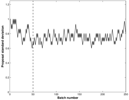
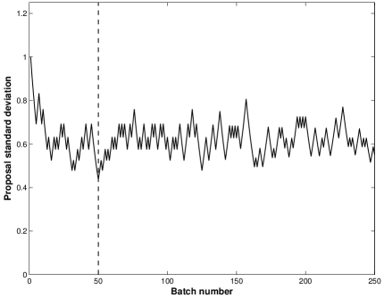
Here we focus on the ability of ESS to find a parsimonious set of predictors in an animal data set (Hubner et al., 2005), where the number of observations, $n=29$, is small with respect to the number of covariates $p=1,421$. This situation, where $n\ll p$, is quite common in animal experiments since environmental sources of variation are controlled as well as the biological diversity of the sample. For illustration, we report the analysis of one gene expression response, where we apply ESS$g$ with and without the hyperprior on $\tau$, see Table 1– eQTL. In the former case, thanks to the adaptive proposal, the Markov chain for $\tau$ mixes very well reaching an overall acceptance rate which is close to the target value $0.44$. Convergence issue is not a problem since the trace of the proposal’s standard deviation stabilises quickly and well inside the bounded conditions, see Figure 3.

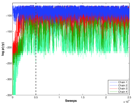
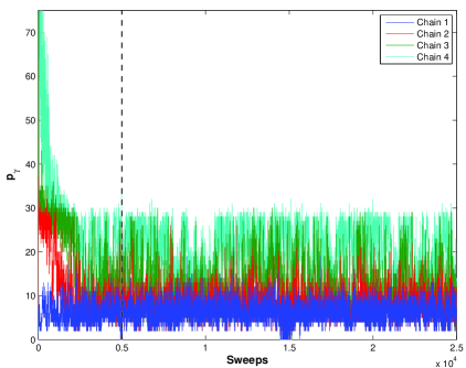
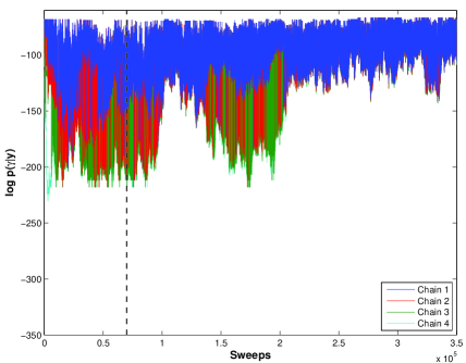
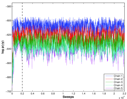
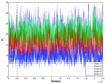
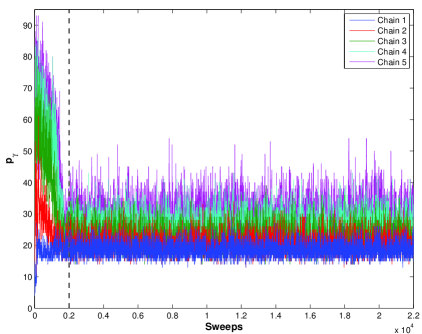
In both cases a good mixing among the $L=4$ chains is obtained (Figure 1, top panels, ESS$g$ with $\tau=29$). Although in the case depicted in Figure 1 with fixed $\tau$, the convergence is reached in the product space $\prod\nolimits_{l=1}^{L}\left[p\left(\gamma_{l}\left|y\right.\right)\right]^{1/t_{l}}$, by visual inspection we see that each chain marginally reaches its equilibrium with respect to the others; moreover, thanks to the automatic tuning of the temperature placement during the burn-in, the distributions of the chains log posterior probabilities overlap nicely, allowing effective exchange of information between the chains. Table 1–eQTL, confirms that the automatic temperature selection works well (with and without the hyperprior on $\tau$) reaching an acceptance rate for the monitored exchange (delayed rejection) operator close to the selected target of $0.50$. The all-exchange operator shows a higher acceptance rate, while, in contrast to Jasra et al. (2007), the overall crossover acceptance rate is reasonable high: in our experience the good performance of the crossover operator is both related to the selection operator (Section 3.1) and the new block crossover which shows an acceptance rate far higher than the others. Finally the computational time on the same desktop computer (see details in Appendix B.3) is rather similar with or without the hyperprior $\tau$, $28$ and $30$ minutes respectively for $25,000$ sweeps with $5,000$ as burn-in.

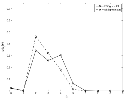
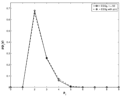
The main difference among the two implementations of ESS$g$ is related to the posterior model size: when $\tau$ is fixed at $\tau=29$ (Unit Information Prior, Fernández et al., 2001), there is more uncertainty and support for larger models, see Figure 2 (a). In both cases we fix $E\left(p_{\gamma}\right)=4$ and $V\left(p_{\gamma}\right)=2$, following prior biological knowledge on the genetic regulation. The posterior mean of the variable selection coefficient is a little smaller than the Unit Information Prior, with ESS$g$ coupled with the Z-S prior favouring smaller models than when $\tau$ is set equal to $29$. The best model visited (and the corresponding $R_{\gamma}^{2}=1-S(\gamma)/y^{T}y$) is the same for both version of ESS$g$, while, when a hyperprior on $\tau$ is implemented, the “stability index” which indicates how much the algorithm persists on the first chain top $1,000$ (not unique) visited models ranked by the posterior probability (Appendix B.3), shows a higher stability, see Table 1– eQTL. In this case, having a data-driven level of shrinkage helps the search algorithm to better discriminate among competing models.

Our second example is related to the application of model (1) in another genomics example: $10,000$ SNPs, selected genome-wide from a candidate gene study, are used to predict the variation of Mass Spectography metabolomics data in a small human population, an example of a so-called mQTL experiment. A suitable dimension reduction of the data is performed to divide the spectra in regions or bins and $\log_{10}$-transformation is applied in order to normalise the signal.

We present the key findings related to a particular metabolite bin, but the same comments can be extended to the analysis of the whole data set, where we regressed every metabolites bin versus the genotype data ($n=50$ and $p=10,000$). In this very challenging case, we still found an efficient mixing of the chains (see Table 1–mQTL). Note that in this case the posterior mean of $\tau$, $63.577$, is a little larger than the Unit Information Prior, $\tau=n$, although the influence of the hyperprior is less important than in the previous real data example, see Figure 2 (b). In both examples, the posterior model size favours clearly polygenic control with significant support for up to four genetic control points (Figure 2) highlighting the advantage of performing multivariate analysis in genomics rather than the traditional univariate analysis.

As expected in view of the very large number of predictors, in the mQTL example the computational time is quite large, around $5$ hours for $20,000$ sweeps after a burn-in of $5,000$, but as shown in Table 1 by the “stability index” ($\approx 0$), we believe that the number of iterations chosen exceeds what is required in order to visit faithfully the model space. For such large data analysis tasks, parallelisation of the code could provide big gains of computer time and would be ideally suited to our multiple chains approach.

[Table 1 about here – Figure 1 about here – Figure 2 about here – Figure 3 about here]

We also evaluate the superiority of our ESS algorithm, and in particular the FSMH scheme and the block crossover, with respect to more traditional EMC implementations illustrated for instance in Liang and Wong (2000). Albeit we believe that using a wide portfolio of different moves enables any searching algorithm to better explore complicated model spaces, we reanalysed the first real data example, eQTL analysis, comparing: (i) ESS$g$ with only FSMH as local move vs ESS with only MC³ as local move; (ii) ESS$g$ with only block crossover vs ESS$g$ with only 1-point, only uniform and only adaptive crossover respectively. To avoid dependency of the results on the initialisation of the algorithm, we replicated the analysis $25$ times. Moreover, to make the comparison fair, in experiment (i) we run the two versions of ESS$g$ for a different number of sweeps ($25,000$ and $350,000$ with $5,000$ and $70,000$ as burn-in respectively), but matching the number of models evaluated. Results are presented in Table 2. We report here the main findings:

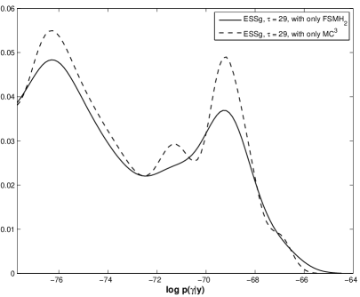
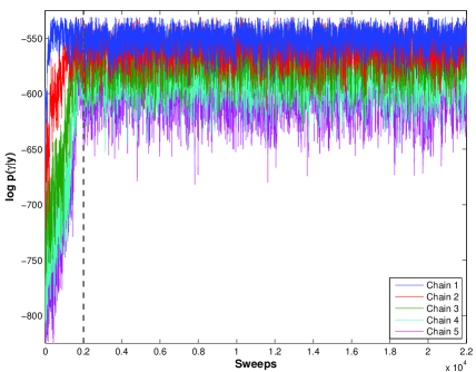
1. over the $25$ runs, ESS$g$ with FSMH reaches the same top visited model $68$% (17/25) while ESS$g$ with MC³ the same top model only $28$%, with a fixed $\tau$, and $88$% and $40$% respectively with Z-S prior. This ability is extended to the top models ranked by the posterior probability, data not shown, providing indirect evidence that the proposed new move helps the algorithm to increase its predictive power. The great superiority when FSMH scheme are implemented can be explained by comparing subplot (a) and (c) in Figure 1: the exchange of information between chains for ESS$g$ with MC³ as local move when $p>n$ (and $p\gg p_{\gamma}$) is rather poor, negating the purpose of EMC. ESS$g$ with MC³ has more difficulties to reach convergence in the product space and, in contrast to ESS$g$ with FSMH, the retained chain does not easily escape from local modes. This later point can be seen looking at Figure 1 (d) which magnifies the right hand tail of the kernel density of $\log p\left(\gamma\left|y\right.\right)$ for the recorded chain, pulling together the $25$ runs: interestingly ESS$g$ with FSMH is less “bumpy”, showing a better ability to escape from local modes and to explore more efficiently the right tail.

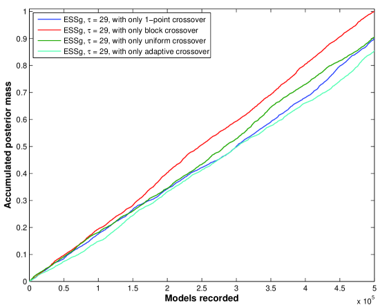
2. Regarding the second comparison when $\tau$ is fixed, ESS$g$ with only block crossover beats constantly the other crossover operators, with $80$% vs about $60$%, in terms of best model visited (Table 2) and models with higher posterior probability (data not shown), has higher acceptance rate (Table 3), showing also a great capacity to accumulate posterior mass as illustrated in Figure 4. The specific benefit of the block crossover is less pronounced when a prior on $\tau$ is specified, but we have already noticed that in this case having a hyperprior on $\tau$ greatly improves the efficiency of the search.

[Table 2 about here – Table 3 about here – Figure 4 about here]

4.2 Simulation study

We briefly report on a comprehensive study of the performance of ESS in a variety of simulated examples as well as a comparison with SSS. To make comparison with SSS fair, we use ESS${i}$, the version of our algorithm which assumes independent priors, $\Sigma_{\gamma}=\tau I_{p_{\gamma}}$,with $\tau$ fixed at $1$. Details of the simulated examples (6 set-ups) and how we conducted the simulation experiment (25 replication of each set-up) are given in Appendix B. The rationale behind the construction of the examples was to benchmark our algorithm against both $n>p$ and $p>n$ cases, to use as building blocks intricate correlation structures that had been used in previous comparisons by G&McC (1993, 1997) and N&G (2004), as well as a realistic correlation structure derived from genetic data, and to include elements of model uncertainty in some of the examples by using a range of values of regression coefficients.

In our example we observe an effective exchange of information between the chains (reported in Table 4) which shows good overall acceptance rates for the collection of moves that we have implemented. The dimension of the problem does not seem to affect the acceptance rates in Table 4, remarkably since values of $p$ range from $60$ to $1,000$ between the examples. We also studied specifically the performance of the global moves (Table 5) to scrutinise our temperature tuning and confirmed the good performance of ESS$i$ with good frequencies of swapping (not far from the case where adjacent chains are selected to swap at random with equal probability) and good measures of overlap between chains.

All the examples were run in parallel with ESS${i}$ and SSS 2.0 (Hans et al., 2007) for the same number of sweeps (22,000) and matching hyperparameters on the model size. Comparison were made with respect to the marginal probability of inclusion as well as the ability to reach models with high posterior probability and to persist in this region. For a detailed discussion of all comparison, see Appendix B.3.

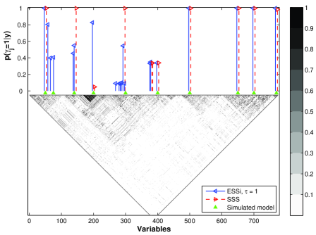
Overall the covariates with non-zero effects have high marginal posterior probability of inclusion for ESS$i$ in all the examples, see Figure 6. There is good agreement between the two algorithms in general, with additional evidence on some examples (Figure 6 (c) and (d)) that ESS$i$ is able to explore more fully the model space and in particular to find small effects, leading to a posterior model size that is close to the true one. Measures of goodness of fit and stability, Table 6, are in good agreement between ESS$i$ and SSS. The comparison highlight that a key feature of SSS, its ability to move quickly towards the right model and to persist on it, is accompanied by a drawback in having difficulty to explore far apart models with competing explanatory power, in contrast to ESS$i$ (contaminated example set-up). Altogether ESS$i$ shows a small improvement of $R_{\gamma}^{2}$, related to its ability to pick up some of the small effects that are missed by SSS. Finally ESS$i$ shows a remarkable superiority in terms of computational time, especially when the simulated (and estimated) $p_{\gamma}$ is large. Altogether our comparisons show that we have designed a fully Bayesian MCMC-EMC sampler which is competitive with the effective search provided by SSS$i$.

In the same spirit of the real data example analysis, we also evaluate the superiority of the FSMH scheme with respect to more traditional EMC implementations, i.e when a MC³ local move is selected. While both versions of the search algorithm visit almost the same top models ranked by the posterior probability, ESS persists more on the top models.

[Table 4 about here – Table 5 about here – Table 6 about here

Figure 5 about here – Figure 6 about here]

5 Discussion

The key idea in constructing an effective MCMC sampler for $\gamma$ and $\tau$ is to add an extra parameter, the temperature, that weakens the likelihood contribution and enables escaping from local modes. Running parallel chains at different temperature is, on the other hand, expensive and the added computational cost has to be balanced against the gains arising from the various “exchanges” between the chains. This is why we focussed on developing a good strategy for selecting the pairs of chains, using both marginal and joint information between the chains, attempting bold and more conservative exchanges. Combining this with an automatic choice of the temperature ladder during burn-in is one of the key element of our ESS algorithm. Using PT in this way has the potential to be effective in a wide range of situations where the posterior space is multimodal.

To tackle the case where $p$ is large with respect to $p_{\gamma}$, the second important element in our algorithm is the use of a Metropolised Gibbs sampling-like step performed on a subset of indices in the local updating of the latent binary vector, rather than an MC³ or RJ-like updating move. The new Fast Scan Metropolis Hastings sampler that we propose to perform these local moves achieves an effective compromise between full Gibbs sampling that is not feasible at every sweep when $p$ is large and vanilla add/delete moves. Comparison of FSMH vs MC³ scheme on a real data example and simulation study shows the superiority of our new local move.

When a model with a prior on the variable selection coefficient $\tau$ is preferred, the updating of $\tau$ itself present no particular difficulties and is computationally inexpensive. Moreover, using an adaptive sampler makes the algorithm self contained without any time consuming tuning of the proposal variance. This latter strategy works perfectly well both in the $g$-prior and independent prior case as illustrated in Sections 4.1 and 4.2. Our current implementation does not make use of the output of the heated chains for posterior inference. Whether gains in variance reduction could be achieved in the spirit of Gramacy et al. (2007) is an area for further exploration, which is beyond the scope of the present work.

Our approach has been applied so far to linear regression with univariate response $y$. An interesting generalisation is that of a multidimensional $n\times q$ response $Y$ and the identification of regressors that jointly predict the $Y$ (Brown et al., 1998). Much of our set-up and algorithm carries through without difficulties and we have already implemented our algorithm in this framework in a challenging case study in genomics with multidimensional outcomes.

Appendix

Appendix A Technical details of EMC implementation

In this Section we will describe some technical details omitted from the paper and related to the sampling schemes we used for the population of binary latent vectors $\bm{\gamma}$ and the selection coefficient $\tau$.

A.1 EMC sampler for $\bm{\gamma}$

Local move: FSMH scheme

Let $\gamma_{l,j}$, $l=1,\ldots,L$ and $j=1,\ldots,p$ to denote the $j$th latent binary indicator in the $l$th chain. As in Kohn et al. (2001), let $\gamma_{l,j}^{\left(1\right)}=\left(\gamma_{l,1},\ldots,\gamma_{l,j-1},\gamma_{l,j}=1,\gamma_{l,j+1},\ldots,\gamma_{l,p}\right)^{T}$ and
$\gamma_{l,j}^{\left(0\right)}=\left(\gamma_{l,1},\ldots,\gamma_{l,j-1},\gamma_{l,j}=0,\gamma_{l,j+1},\ldots,\gamma_{l,p}\right)^{T}$. Furthermore let $L_{l,j}^{\left(1\right)}\propto p\left(y\left|\gamma_{l,j}^{\left(1\right)},\tau\right.\right)$ and $L_{l,j}^{\left(0\right)}\propto p\left(y\left|\gamma_{l,j}^{\left(0\right)},\tau\right.\right)$ and finally $\theta_{l,j}^{\left(1\right)}=p\left(\gamma_{l,j}=1\left|\gamma_{l,j^{-}}\right.\right)$ and $\theta_{l,j}^{\left(0\right)}=1-\theta_{l,j}^{\left(1\right)}$. From (6) it is easy to prove that

$$\theta_{l,j}^{\left(1\right)}=p\left(\gamma_{l,j}=1\left|\gamma_{l,j^{-}}\right.\right)=\frac{p_{\gamma_{l}}+a_{\omega}-1}{p+a_{\omega}+b_{\omega}-1},$$ (A.1)

where $p_{\gamma_{l}}$ is the current model size for the $l$th chain. Using the above equation, for $\gamma_{l,j}=1$ the normalised version of (12) can be written as

$$\left[p\left(\gamma_{l,j}=1\left|y,\gamma_{l,j^{-}},\tau\right.\right)\right]^{1/t_{l}}=\frac{\left.\theta_{l,j}^{\left(1\right)}\right.^{1/t_{l}}\left.L_{l,j}^{\left(1\right)}\right.^{1/t_{l}}}{S\left(1/t_{l}\right)},$$ (A.2)

where $S\left(1/t_{l}\right)=\left.\theta_{l,j}^{\left(1\right)}\right.^{1/t_{l}}\left.L_{l,j}^{\left(1\right)}\right.^{1/t_{l}}+\left.\theta_{l,j}^{\left(0\right)}\right.^{1/t_{l}}\left.L_{l,j}^{\left(0\right)}\right.^{1/t_{l}}$ with $\left[p\left(\gamma_{l,j}=1\left|y,\gamma_{l,j^{-}},\tau\right.\right)\right]^{1/t_{l}}$ defined similarly. Hence if $\left.\theta_{l,j}^{\left(1\right)}\right.^{1/t_{l}}$ is very small, then $\left[p\left(\gamma_{l,j}=1\left|y,\gamma_{l,j^{-}},\tau\right.\right)\right]^{1/t_{l}}$ is small as well. Therefore for the Gibbs sampler with a beta-binomial prior on the model space, the posterior probability of $\gamma_{l,j}=1$ depends crucially on $\left.\theta_{l,j}^{\left(1\right)}\right.^{1/t_{l}}$.

In the following we derive a Fast Scan Metropolis-Hastings scheme specialised for Evolutionary Monte Carlo or parallel tempering. We define $Q\left(1\rightarrow 0\right)=Q\left(\gamma_{l,j}^{\left(1\right)}\rightarrow\gamma_{l,j}^{\left(0\right)}\right)$ as the proposal probability to go from $1$ to $0$ and $Q\left(0\rightarrow 1\right)$ the proposal probability to go from $0$ to $1$ for the $j$th variable and $l$th chain. Moreover using the notation introduced before, the Metropolis-within-Gibbs version of (12) to go from $0$ to $1$ in the EMC local move is

$$\alpha_{l}^{\text{MwG}}\left(0\rightarrow 1\right)=\min\left\{1,\frac{\left.\theta_{l,j}^{\left(1\right)}\right.^{1/t_{l}}\left.L_{l,j}^{\left(1\right)}\right.^{1/t_{l}}}{\left.\theta_{l,j}^{\left(0\right)}\right.^{1/t_{l}}\left.L_{l,j}^{\left(0\right)}\right.^{1/t_{l}}}\frac{Q\left(1\rightarrow 0\right)}{Q\left(0\rightarrow 1\right)}\right\}$$ (A.3)

with a similar expression for $\alpha_{l}^{\text{MwG}}\left(1\rightarrow 0\right)$. The proof of the Propositions are omitted since they are easy to check. We first introduce the following Proposition which is useful for the calculation of the acceptance probability in the FSMH scheme.

Proposition 1

The following three conditions are equivalent: a) $\left.L_{l,j}^{\left(0\right)}\right.^{1/t_{l}}\left.\left/L_{l,j}^{\left(1\right)}\right.^{1/t_{l}}\geq 1\right.$;
b) $\left.L_{l,j}^{\left(1\right)}\right.^{1/t_{l}}\left/\tilde{S}\left(1/t_{l}\right)\geq 1\right.$; c)$\left.L_{l,j}^{\left(0\right)}\right.^{1/t_{l}}\left/\tilde{S}\left(1/t_{l}\right)<1\right.$, where $\tilde{S}\left(1/t_{l}\right)=S\left(1/t_{l}\right)\left/\left(\left.\theta_{l,j}^{\left(1\right)}\right.^{1/t_{l}}+\left.\theta_{l,j}^{\left(0\right)}\right.^{1/t_{l}}\right)\right.$ is the convex combination of the marginal likelihood $\left.L_{l,j}^{\left(1\right)}\right.^{1/t_{l}}$ and $\left.L_{l,j}^{\left(0\right)}\right.^{1/t_{l}}$ with weights $\tilde{\theta}_{l,j}^{\left(1\right)}\left(1/t_{l}\right)=\left.\theta_{l,j}^{\left(1\right)}\right.^{1/t_{l}}\left/\left(\left.\theta_{l,j}^{\left(1\right)}\right.^{1/t_{l}}+\left.\theta_{l,j}^{\left(0\right)}\right.^{1/t_{l}}\right)\right.$ and $\tilde{\theta}_{l,j}^{\left(0\right)}\left(1/t_{l}\right)=1-\tilde{\theta}_{l,j}^{\left(1\right)}\left(1/t_{l}\right)$.

The FSMH scheme can be seen as a random scan Metropolis-within-Gibbs algorithm where the number of evaluations is linked to the prior/current model size and the temperature attached to the chain. The computation requirement for the additional acceptance/rejection step is very modest since the normalised tempered version of (A.1) is used.

Proposition 2

Let $l=1,\ldots,L$, $j=1,\ldots,p$ (or any permutation of them), $Q^{\text{FSMH}}\left(0\rightarrow 1\right)=\tilde{\theta}_{l,j}^{\left(1\right)}\left(1/t_{l}\right)$ and $Q^{\text{FSMH}}\left(1\rightarrow 0\right)=\tilde{\theta}_{l,j}^{\left(0\right)}\left(1/t_{l}\right)$ with $\tilde{\theta}_{l,j}^{\left(0\right)}\left(1/t_{l}\right)=1-\tilde{\theta}_{l,j}^{\left(1\right)}\left(1/t_{l}\right)$. The acceptance probabilities are

$$\alpha_{l}^{\text{FSMH}}\left(0\rightarrow 1\right)=\left\{\begin{tabular}[]{ll}$1$&$\text{if }\left.L_{l,j}^{\left(1\right)}\right.^{1/t_{l}}\left/\left.L_{l,j}^{\left(0\right)}\right.^{1/t_{l}}\right.\geq 1$\\ $\left.L_{l,j}^{\left(1\right)}\right.^{1/t_{l}}\left/\left.L_{l,j}^{\left(0\right)}\right.^{1/t_{l}}\right.$&$\text{if }\left.L_{l,j}^{\left(1\right)}\right.^{1/t_{l}}\left/\left.L_{l,j}^{\left(0\right)}\right.^{1/t_{l}}\right.<1$\end{tabular}\right.$$ (A.4)

$$\alpha_{l}^{\text{FSMH}}\left(1\rightarrow 0\right)=\left\{\begin{tabular}[]{ll}$1$&$\text{if }\left.L_{l,j}^{\left(0\right)}\right.^{1/t_{l}}\left/\left.L_{l,j}^{\left(1\right)}\right.^{1/t_{l}}\right.\geq 1$\\ $\left.L_{l,j}^{\left(0\right)}\right.^{1/t_{l}}\left/\left.L_{l,j}^{\left(1\right)}\right.^{1/t_{l}}\right.$&$\text{if }\left.L_{l,j}^{\left(0\right)}\right.^{1/t_{l}}\left/\left.L_{l,j}^{\left(1\right)}\right.^{1/t_{l}}<1\right.$\end{tabular}\right.$$ (A.5)

The above sampling scheme works as follows. Given the $l$th chain, if $\gamma_{lj}=0$ (and similarly for $\gamma_{lj}=1$), it proposes the new value from a Bernoulli distribution with probability $\tilde{\theta}_{l,j}^{\left(1\right)}\left(1/t_{l}\right)$: if the proposed value is different from the current one, it evaluates (A.4) (and similarly A.5)otherwise it selects a new covariate.

Finally it can be proved that the Gibbs sampler is more efficient than the FSMH scheme, i.e. for a fixed number of iterations, Gibbs sampling MCMC standard error is lower than for FSMH sampler. However the Gibbs sampler is computationally more expensive so that, if $p$ is very large, as described in Kohn et al. (2001), FSMH scheme becomes more efficient per floating point operation.

Global move: exchange operator

The exchange operator can be seen as an extreme case of crossover operator, where the first proposed chain receives the whole second chain state $\gamma_{l}^{\prime}=\gamma_{r}$, and the second proposed chain receives the whole first state chain $\gamma_{r}^{\prime}=\gamma_{l}$, respectively.

In order to achieve a good acceptance rate, the exchange operator is usually applied on adjacent chains in the temperature ladder, which limits its capacity for mixing. To obtain better mixing, we implemented two different approaches: the first one is based on Jasra et al. (2007) and the related idea of delayed rejection (Green and Mira, 2001); the second one on Gibbs distribution over all possible chains pairs (Calvo, 2005).

1. The delayed rejection exchange operator tries first to swap the state of the chains that are usually far apart in the temperature ladder, but, once the proposed move has been rejected, it performs a more traditional (uniform) adjacent pair selection, increasing the overall mixing between chains on one hand without drastically reducing the acceptance rate on the other. However its flexibility comes at some extra computational costs and in particular the additional evaluation of the pseudo move necessary to maintain detailed balance (Green and Mira, 2001). Details are reported below.

   Suppose two chains are selected at random, $l$ and $r$ with $l\neq r$, in order to swap their binary latent vector. Then, given that $\gamma_{l}^{\prime}=\gamma_{r}$, $\gamma_{r}^{\prime}=\gamma_{l}$ and $Q_{t}\left(\bm{\gamma}\rightarrow\bm{\gamma}^{\prime}\right)=Q_{t}\left(\bm{\gamma}^{\prime}\rightarrow\bm{\gamma}\right)$, (13) reduces to

   $$\alpha_{1}\left(\bm{\gamma}\rightarrow\bm{\gamma}^{\prime}\right)=\min\left\{1,\frac{\exp\left\{f\left(\gamma_{r}\left|\tau\right.\right)/t_{l}+f\left(\gamma_{l}\left|\tau\right.\right)/t_{r}\right\}}{\exp\left\{f\left(\gamma_{l}\left|\tau\right.\right)/t_{l}+f\left(\gamma_{r}\left|\tau\right.\right)/t_{r}\right\}}\right\}.$$

   Since the two chains are selected at random, the above acceptance probability decreases exponentially with the difference $\left|1/t_{l}-1/t_{r}\right|$ and therefore most of the proposed moves are rejected. If rejected, a delayed rejection-type move is applied between two random adjacent chains, with $l$ the first one and $s$, $\left|l-s\right|=1$, the second one, giving rise to the new acceptance probability

   $$\alpha_{2}\left(\bm{\gamma}\rightarrow\bm{\gamma}^{\prime\prime}\right)=\min\left\{1,\frac{\exp\left\{f\left(\gamma_{s}\left|\tau\right.\right)/t_{l}+f\left(\gamma_{l}\left|\tau\right.\right)/t_{s}\right\}}{\exp\left\{f\left(\gamma_{l}\left|\tau\right.\right)/t_{l}+f\left(\gamma_{s}\left|\tau\right.\right)/t_{s}\right\}}\frac{1-\alpha_{1}\left(\bm{\gamma}^{\prime\prime}\rightarrow\bm{\gamma}^{\ast}\right)}{1-\alpha_{1}\left(\bm{\gamma}\rightarrow\bm{\gamma}^{\prime}\right)}\right\},$$

   where the pseudo move $\bm{\gamma}^{\ast}$ is necessary in order to maintain the detailed balance condition (Green and Mira, 2001).

2. Alternatively, we attempt a bolder “all-exchange” operator. Swapping the state of two chains that are far apart in the temperature ladder speeds up the convergence of the simulation since it replaces several adjacent swaps with a single move. However, this move can be seen as a rare event whose acceptance probability is low and unknown. Since the full set of possible exchange moves is finite and discrete, it is easy and computationally inexpensive to calculate all the $L\left(L-1\right)/2$ exchange acceptance rates between all chains pairs, inclusive the rare ones, $\tilde{p}_{l,r}=\exp\left\{\left(f\left(\gamma_{r}\left|\tau\right.\right)-f\left(\gamma_{l}\left|\tau\right.\right)\right)\left(1/t_{l}-1/t_{r}\right)\right\}$. To maintain detailed balance condition, the possibility not to perform any exchange (rejection) must be added with unnormalised probability one. Finally the chains whose states are swopped are selected at random with probability equal to

   $$p_{h}=\frac{\tilde{p}_{h}}{\sum_{h=1}^{1+L\left(L-1\right)/2}\tilde{p}_{h}},$$ (A.6)

   where in (A.6) each pair $\left(l,r<l\right)$ is denoted by a single number $h$, $\tilde{p}_{h}=\tilde{p}_{l,r}$, including the rejection move, $h=1$.

Temperature placement

First we select the number $L$ of chains close to the complexity of the problem, i.e. $E\left(p_{\gamma}\right)$, although the size of the data and computational limits need to be taken into account. Secondly, we fix a first stage temperature ladder according to a geometric scale such that $t_{l+1}/t_{l}=b$, $b>1$, $l=1,\ldots,L$ with $b$ relatively large, for instance $b=4$. Finally, we adopt a strategy similar to the one described in Roberts and Rosenthal (2008), but restricted to the burn-in stage, monitoring only the acceptance rate of the delayed rejection exchange operator. After the $k$th “batch” of EMC sweeps, to be chosen but usually set equal to $100$, we update $b_{k}$, the value of the constant $b$ up to the $k$th batch, by adding or subtracting an amount $\delta_{b}$ such that the acceptance rate of the delayed rejection exchange operator is as close as possible to $0.50$ (Liu, 2001; Jasra et al., 2007), $b_{k+1}=2^{\log_{2}b_{k}\pm\delta_{b}}$. Specifically the value of $\delta_{b}$ is chosen such that at the end of the burn-in period the value of $b$ can be 1. To be precise, we fix the value of $\delta_{b}$ as $\log_{2}\left(b_{1}\right)/\tilde{K}$, where $b_{1}$ is the first value assigned to the geometric ratio and $\tilde{K}$ is the total number of batches in the burn-in period.

A.2 Adaptive Metropolis-within-Gibbs for $\tau$

Laplace approximation for the conditional marginal likelihood

Under model (1) and prior specification for $\alpha$, (2) and (3), we provide the Laplace approximation of $p\left(y\left|\gamma,\tau\right.\right)$ for the $g$-prior case, while the approximation for the independent case can be derived following the same line of reasoning. For easy of notation we drop the chain subscript index and we assume that the observed responses $y$ have been centred with mean $0$, i.e. $\left(y-\bar{y}_{n}\right)\equiv y$. In the following we will distinguish the cases in which the posterior mode $\hat{\tau}_{\gamma}$ is a solution of a cubic or quadratic equation. Conditions on the existence of the solutions are provided as well as those that guarantee the positive semidefiniteness of the variance approximation. Recall that

$$p\left(y\left|\gamma\right.\right) = \int\exp\left\{\log\left(p\left(y\left|\gamma,\tau\right.\right)p\left(\tau\right)\right)\right\}d\tau$$

$$\approx \sqrt{2\pi}\sigma_{\hat{\lambda}}\left(\log p\left(y\left|\gamma,\hat{\lambda}\right.\right)+\log p\left(\hat{\lambda}\right)+\log J\left(\hat{\lambda}\right)\right),$$

where $\hat{\lambda}$ is the posterior mode after the transformation $\lambda=\log\left(\tau\right)$, which is necessary to avoid problems on the boundary, $\sigma_{\hat{\lambda}}$ is the approximate squared root of the variance calculated in $\hat{\lambda}$ and $J\left(\cdot\right)$ is the Jacobian of the transformation. Details about Laplace approximation can be found in Tierney and Kadane (1986). Similar derivations when $p\left(\sigma^{2}\right)\propto\sigma^{-2}$ are presented in Liang et al. (2008). Finally throughout the presentation we will assume that $n>p_{\gamma}$ and that $a_{g}$ and $b_{g}$ are fixed small as in Kohn et al. (2001).

Cubic equation for Zellner-Siow priors
If $p\left(\tau\right)=InvGa\left(a_{\tau},b_{\tau}\right)$ the posterior $\hat{\lambda}$ mode is the only positive root of the integrand function

$$I_{\lambda}=\left(1+e^{\lambda}\right)^{\left(2a_{\sigma}+n-1-p_{\gamma}\right)/2}\left\{2b_{\sigma}\left(1+e^{\lambda}\right)+y^{T}y\left[1+e^{\lambda}\left(1-R_{\gamma}^{2}\right)\right]\right\}^{-\left(2a_{\sigma}+n-1\right)/2}\frac{e^{-b_{\tau}/e^{\lambda}}}{\left(e^{\lambda}\right)^{a_{\tau}+1}}e^{\lambda},$$

where the last factor in the above equation $e^{\lambda}=\left|de^{\lambda}/d\lambda\right|$ is the Jacobian of the transformation. After the calculus of the first derivative of the log transformation and some algebra manipulations, it can be shown that $e^{\hat{\lambda}}$ is the solution of the cubic equation

$$e^{3\lambda}+\frac{c_{1}c_{3}-c_{2}c_{4}-\left(c_{3}+c_{4}\right)a_{\tau}+c_{4}b_{\tau}}{\left(c_{1}-c_{2}-a_{\tau}\right)c_{4}}e^{2\lambda}+\frac{-c_{3}a_{\tau}+\left(c_{3}+c_{4}\right)b_{\tau}}{\left(c_{1}-c_{2}-a_{\tau}\right)c_{4}}e^{\lambda}+\frac{c_{3}b_{\tau}}{\left(c_{1}-c_{2}-a_{\tau}\right)c_{4}}=0$$ (A.7)

and that

$$\sigma_{\hat{\lambda}}^{2} = \left.-\frac{1}{\left(\log p\left(y\left|\gamma,\lambda\right.\right)+\log p\left(\lambda\right)\right)^{\prime\prime}}\right|_{\lambda=\hat{\lambda}}$$ (A.8)

$$= \left[-c_{1}\frac{e^{\lambda}}{\left(1+e^{\lambda}\right)^{2}}+c_{2}\frac{c_{3}c_{4}e^{\lambda}}{\left(c_{3}+c_{4}e^{\lambda}\right)^{2}}+\frac{b_{\tau}}{e^{\lambda}}\right]_{\lambda=\hat{\lambda}}^{-1},$$

where $c_{1}=\left(2a_{\sigma}+n-1-p_{\gamma}\right)/2$, $c_{2}=\left(2a_{\sigma}+n-1\right)/2$, $c_{3}=2b_{\sigma}+y^{T}y$ and $c_{4}=2b_{\sigma}+y^{T}y\left(1-R_{\gamma}^{2}\right)$. Following Liang et al. (2008), since $\lim_{\lambda\rightarrow-\infty}\partial I_{\lambda}/\partial\lambda>0$, because $c_{3}b_{\tau}>0$, and $\lim_{\lambda\rightarrow\infty}\partial I_{\lambda}/\partial\lambda<0$, because $\left(c_{1}-c_{2}-a_{\tau}\right)c_{4}<0$, at least one real positive solution exists. Moreover since $-\left(c_{3}b_{\tau}\right)/\left(c_{1}-c_{2}-a_{\tau}\right)c_{4}>0$, the remaining two real solutions should have the same sign (Abramowitz and Stegun, 1970). A necessary condition for the existence of just one real positive solution is that the summation of all the pairs-products of the coefficients is negative

$$\frac{-c_{3}a_{\tau}+\left(c_{3}+c_{4}\right)b_{\tau}}{\left(c_{1}-c_{2}-a_{\tau}\right)c_{4}}<0$$

and this happens if $b_{\tau}/a_{\tau}>c_{3}/\left(c_{3}+c_{4}\right)$. When $R_{\gamma}^{2}\rightarrow 0$ and thus $c_{3}=c_{4}$, the above condition corresponds to $b_{\tau}>a_{\tau}/2$ and when $R_{\gamma}^{2}\rightarrow 1$, as $c_{3}/\left(c_{3}+c_{4}\right)\approx 1$ especially when $y^{T}y$ is large, which might be expected when $n$ becomes large, the condition is equivalent to $b_{\tau}>a_{\tau}$. Therefore it turns out that a sufficient condition for the existence of just one real positive solution in (A.1) is $b_{\tau}>a_{\tau}$.

The positive semidefiniteness of the approximate variance can be proved as follows. First of all it is worth noticing that all the terms in (A.8) are of the same order $O_{p}\left(e^{-\lambda}\right)$. Then, when $R_{\gamma}^{2}\rightarrow 0$, the positive semidefiniteness is always guaranteed, while when $R_{\gamma}^{2}\rightarrow 1$, provided that $y^{T}y$ is large, the middle term in (A.8) tends to zero and the condition is fulfilled if $b_{\tau}>c_{1}$.

Quadratic equation for Liang et al. (2008) prior
If $p\left(\tau\right)\propto\left(1+\tau\right)^{-c_{\tau}}$, with $c_{\tau}>0$, $e^{\hat{\lambda}}$ is only the positive root of the integrand function

$$I_{\lambda}=\left(1+e^{\lambda}\right)^{\left(2a_{\sigma}+n-1-p_{\gamma}-c_{\tau}\right)/2}\left\{2b_{\sigma}\left(1+e^{\lambda}\right)+y^{T}y\left[1+e^{\lambda}\left(1-R_{\gamma}^{2}\right)\right]\right\}^{-\left(2a_{\sigma}+n-1\right)/2}e^{\lambda}$$

or, after the first derivative of the log transformation, the solution of the quadratic equation

$$\left(c_{1}^{\ast}-c_{2}+1\right)c_{4}e^{2\lambda}+\left(c_{1}^{\ast}c_{3}-c_{2}c_{4}+c_{3}+c_{4}\right)e^{\lambda}+c_{3}=0$$ (A.9)

with $c_{1}^{\ast}=\left[2a_{\sigma}+n-1-\left(p_{\gamma}+2c_{\tau}\right)\right]/2$ and $c_{2}$, $c_{3}$ and $c_{4}$ defined as above. The discriminant of the quadratic equation is $\Delta=\left(c_{1}^{\ast}c_{3}-c_{2}c_{4}c_{3}+c_{3}+c_{4}\right)^{2}-4\left(c_{1}^{\ast}-c_{2}+1\right)c_{4}c_{3}$ which is always greater than zero and therefore two real roots exist. Since one of them is positive in order to prove that (A.9) admits just one positive solution, it is necessary to show that

$$\frac{-\left(c_{1}^{\ast}c_{3}-c_{2}c_{4}+c_{3}+c_{4}\right)-\Delta^{1/2}}{2\left(c_{1}^{\ast}-c_{2}+1\right)c_{4}}<0$$

which is true provided that $\left(c_{1}^{\ast}-c_{2}+1\right)c_{4}c_{3}<0$. Moreover the approximate variance can be written as

$$\sigma_{\hat{\lambda}}^{2}=\left[-c_{1}^{\ast}\frac{e^{\lambda}}{\left(1+e^{\lambda}\right)^{2}}+c_{2}\frac{c_{3}c_{4}e^{\lambda}}{\left(c_{3}+c_{4}e^{\lambda}\right)^{2}}\right]_{\lambda=\hat{\lambda}}^{-1}$$ (A.10)

which is positive semidefinite when $R_{\gamma}^{2}\rightarrow 0$ if $c_{2}>c_{1}^{\ast}$, which is always verified, while, if $R_{\gamma}^{2}\rightarrow 1$ and $y^{T}y$ is large, equation (A.10) is not positive unless $p_{\gamma}+2c_{\tau}>2a_{\sigma}+n-1$.

The explicit solution of the posterior mode is also available

$$\hat{\tau}_{\gamma} = \max\left\{\frac{\left(c_{4}-c_{3}\right)/\left(c_{1}^{\ast}-c_{2}\right)}{c_{4}/c_{1}^{\ast}}-1,0\right\}$$ (A.11)

$$= \max\left\{\frac{R_{\gamma}^{2}/\left(p_{\gamma}+2c_{\tau}\right)}{\left[2b_{\sigma}/\left(y^{T}y\right)+\left(1-R_{\gamma}^{2}\right)\right]/\left[2a_{\sigma}+n-1-\left(p_{\gamma}+2c_{\tau}\right)\right]}-1,0\right\}$$

which corresponds to MLE if $c_{\tau}=0$.

Diminishing adaptive and bounded conditions

Since $\tau$ is defined on the real positive axis we propose the new value of $\tau$ on the logarithm scale. In particular we use as proposal the normal distribution centred at the current value of $\log\left(\tau\right)$ in the $g$-prior and independent prior case. The variance of the proposal distribution is controlled as illustrated in Roberts and Rosenthal (2008): every $100$ EMC sweeps, the same value of sweeps used in the temperature placement, we monitor the acceptance rate of the Metropolis-within-Gibbs algorithm: if it is lower (higher) than the optimal acceptance rate, i.e. 0.44, a constant $\delta_{\tau}(k)$ is added (subtracted) to $ls_{k}$, the log standard deviation of the proposal distribution in the $k$th batch of EMC sweeps. The value of the constant to be added or subtracted is rather arbitrary, but we found useful to fix it as $\left|ls_{1}-5\right|/\tilde{K}$, where $\tilde{K}$ is the total number of batches in the burn-in period: during the burn-in the log standard deviation should be able to reach any values at a distance $\pm 5$ in log scale from the initial value of $ls_{1}$ usually set equal to zero. The diminishing adaptive condition is obtained imposing $\delta_{\tau}\left(k\right)=\min\{\left|ls_{1}-5\right|/\tilde{K},k^{-1/2}\}$, where $k$ is the current number of batches, including the burn-in. To ensure the bounded convergence condition we follow Roberts and Rosenthal (2008), restricting each $ls_{k}$ to be inside $\left[M_{1},M_{2}\right]$ and we fix them equal to $M_{1}=-10$ and $M_{2}=10$ respectively. In practise these bounds do not create any restriction since the sequence of the standard deviations of the proposal distribution stabilises almost immediately, indicating that the transition kernel converges in a bounded number of batches, see Figure 2.

Appendix B Performance of ESS: Simulation study

In this Section we report in details on the performance of ESS in a variety of simulated examples. Main conclusions are summarised in the Section 4.2.

Firstly we analyse the simulated examples with ESS${i}$ the version of our algorithm which assumes independent priors, $\Sigma_{\gamma}=\tau I_{p_{\gamma}}$, so as to enable comparisons with SSS which also implements an independent prior. Moreover, in order to make to comparison with SSS fair, in the simulation study only the first step of the algorithm described in Section 3.3 is performed, with $\tau$ fixed at $1$. As in SSS, standardisation of the covariates is done before running ESS${i}$. We run ESS${i}$ and SSS 2.0 (Hans et al., 2007) for the same number of sweeps (22,000) and with matching hyperparameters on the model size.

Secondly, to discuss the mixing properties of ESS when a prior $p\left(\tau\right)$ is defined on $\tau$, we implement both the $g$-prior and independent prior set-up for a particular simulated experiment. To be precise in the former case we will use the Zellner-Siow priors (8), and for the latter we will specify a proper but diffuse exponential distribution as suggested by Bae and Mallick (2004).

B.1 Simulated experiments

We apply ESS with independent priors to an extensive and challenging range of simulated examples with $\tau$ fixed at $1$: the first three examples (Ex1-Ex3) consider the case $n>p$ while the remaining three (Ex4-Ex6) have $p>n$. Moreover in all examples, except the last one, we simulate the design matrix, creating more and more intricated correlation structures between the covariates in order to test the proposed algorithm in different and increasingly more realistic scenarios. In the last example, we use, as design matrix, a genetic region spanning $500$-kb from the HapMap project (Altshuler et al., 2005).

Simulated experiments Ex1-Ex5 share in common the way we build $X$. In order to create moderate to strong correlation, we found useful referring to two simulated examples in George and McCulloch, G&McC hereafter, (1993) and in G&McC (1997): throughout we call $X_{1}$ ($n\times 60$) and $X_{2}$ $(n\times 15)$ the design matrix obtained from these two examples. In particular the $j$th column of $X_{1}$, indicated as $X_{\left(1\right)j}$, is simulated as $X_{\left(1\right)j}=X_{j}^{\ast}+Z$, where $X_{1}^{\ast},\ldots,X_{60}^{\ast}$ iid $\sim N_{n}\left(0,1\right)$ independently form $Z\sim N_{n}\left(0,1\right)$, inducing a pairwise correlation of $0.5$. $X_{2}$ is generated as follows: firstly we simulated $Z_{1},\ldots,Z_{15}$ iid $\sim N_{n}\left(0,1\right)$ and we set $X_{\left(2\right)j}=Z_{i}+2Z_{j}$ for $j=1,3,5,8,9,10,12,13,14,15$ only. To induce strong multicollinearity, we then set $X_{\left(2\right)2}=X_{\left(2\right)1}+0.15Z_{2}$, $X_{\left(2\right)4}=X_{\left(2\right)3}+0.15Z_{4}$, $X_{\left(2\right)6}=X_{\left(2\right)5}+0.15Z_{6}$, $X_{\left(2\right)7}=X_{\left(2\right)8}+X_{\left(2\right)9}-X_{\left(2\right)10}+0.15Z_{7}$ and $X_{\left(2\right)11}=X_{\left(2\right)14}+X_{\left(2\right)15}-X_{\left(2\right)12}-X_{\left(2\right)13}+0.15Z_{11}$. A pairwise correlation of about 0.998 between $X_{\left(2\right)j}$ and $X_{\left(2\right)j+1}$ for $j=1,3,5$ is introduced and similarly strong linear relationship is present within the sets $\left(X_{\left(2\right)7},X_{\left(2\right)8},X_{\left(2\right)9},X_{\left(2\right)10}\right)$ and $\left(X_{\left(2\right)11},X_{\left(2\right)12},X_{\left(2\right)13},X_{\left(2\right)14},X_{\left(2\right)15}\right)$.

Then, as in Nott and Green, N&G hereafter, (2004) Example 2, more complex structures are created by placing side by side combinations of $X_{1}$ and/or $X_{2}$, with different sample size. We will vary the number of samples $n$ in $X_{1}$ and $X_{2}$ as we construct our examples. The levels of $\beta$ are taken from the simulation study of Fernández et al. (2001), while the number of true effects, $p_{\gamma}$, with the exception of Ex3, varies from $5$ to $16$. Finally the simulated error variance ranges from $0.05^{2}$ to $2.5^{2}$ in order to vary the level of difficulty for the search algorithm. Throughout we only list the non-zero $\beta_{\gamma}$ and assume that $\beta_{\gamma^{-}}=0^{T}$. The six examples can be summarised as follows:

• $X=X_{1}$ is a matrix of dimension $120\times 60$, where the responses are simulated from (1) using $\alpha=0$, $\gamma=\left(21,37,46,53,54\right)^{T}$, $\beta_{\gamma}=\left(2.5,0.5,-1,1.5,0.5\right)^{T}$, and $\varepsilon\sim N\left(0,2^{2}I_{120}\right)$. In the following we will not refer to the intercept $\alpha$ any more since, as described in Section 3.3 in the paper, we consider $y$ centred and hence there is no difference in the results if the intercept is simulated or not. This is the simplest of our example, although, as reported in G&McC (1993) the average pairwise correlation is about $0.5$, making it already hard to analyse by standard stepwise methods.

• This example is taken directly from N&G (2004), Example 2, who first introduce the idea of combining simpler “building blocks” to create a new matrix $X$ : in their example $X=\left[X_{2}^{\left(1\right)}X_{2}^{\left(2\right)}\right]$ is a $300\times 30$ matrix, where $X_{2}^{\left(1\right)}$ and $X_{2}^{\left(2\right)}$ are of dimension $300\times 15$ and have each the same structure as $X_{2}$. Moreover $\gamma=\left(1,3,5,7,8,11,12,13\right)^{T}$, $\beta_{\gamma}=\left(1.5,1.5,1.5,1.5,-1.5,1.5,1.5,1.5\right)^{T}$ and $\varepsilon\sim N\left(0,2.5^{2}I_{300}\right)$. We chose this example for two reasons: firstly, since the correlation structure in $X_{2}$ is very involved, we test the proposed algorithm under strong and complicated correlations between the covariates; secondly, since $y$ is not simulated from the second “block”, we are interested to see if the proposed algorithm does not select any variable that belongs to the second group.

• As in G&McC (1993), Example 2, $X=X_{1}$, is a $120\times 60$ matrix, $\beta=\left(\beta_{1},\ldots,\beta_{60}\right)^{T}$, $\left(\beta_{1},\ldots,\beta_{15}\right)=\left(0,\ldots,0\right)$, $\left(\beta_{16},\ldots,\beta_{30}\right)=\left(1,\ldots,1\right)$, $\left(\beta_{31},\ldots,\beta_{45}\right)=\left(2,\ldots,2\right)$, $\left(\beta_{46},\ldots,\beta_{60}\right)=\left(3,\ldots,3\right)$ and $\varepsilon\sim N\left(0,2^{2}I_{120}\right)$. The motivation behind this example is to test the strength of the proposed algorithm to select a subset of variables which is large with respect to $p$ while preserving the ability not to choose any of the first $15$ variables.

• The design matrix $X$, $120\times 300$, is constructed as follows: firstly we create a new $120\times 60$ “building block”, $X_{3}$, combining $X_{2}$ and a smaller version of $X_{1}$, $X_{1}^{\ast}$, a $120\times 45$ matrix simulated as $X_{1}$, such that $X_{3}=\left[X_{2}X_{1}^{\ast}\right]$ (dimension $120\times 60$). Secondly we place side by side five copies of $X_{3}$, $X=\left[X_{3}^{\left(1\right)}X_{3}^{\left(2\right)}X_{3}^{\left(3\right)}X_{3}^{\left(4\right)}X_{3}^{\left(5\right)}\right]$: the new design matrix alternates blocks of covariates of high and complicated correlation, as in G&McC (1997), with regions where the correlation is moderate as in G&McC (1993). We simulate the response selecting $16$ variables from $X$,
  $\gamma=\left(1,11,30,45,61,71,90,105,121,131,150,165,181,191,210,225\right)^{T}$ such that every pair belongs alternatively to $X_{2}$ or $X_{1}$. We simulate $y$ using
  $\beta_{\gamma}=\left(2,-1,1.5,1,0.5,2,-1,1.5,1,0.5,2,-1,-1,1.5,1,0.5\right)^{T}$ with $\varepsilon\sim N\left(0,2.5^{2}I_{120}\right)$. This example is challenging in view of the correlation structure, the number of covariates $p>n$ and the different levels of the effects.

• This is the most challenging example that we simulated and it is based on the idea of contaminated models. The matrix $X$, $200\times 1000$, is $X=\left[X_{3}^{\left(1\right)}X_{3}^{\left(2\right)}X_{3}^{\left(3\right)}X_{1}^{\ast\ast}X_{3}^{\left(4\right)}X_{3}^{\left(5\right)}X_{3}^{\left(6\right)}X_{3}^{\left(7\right)}X_{3}^{\left(8\right)}\right]$, with $X_{1}^{\ast\ast}$, a $200\times 520$ larger version of $X_{1}$. We partitioned the responses such that $y=[y_{1}y_{2}]^{T}$: $y_{1}$ is simulated from “model 1” ($\gamma^{1}=\left(701,730,745,763,790,805,825,850,865,887\right)$ and $\beta_{\gamma}^{1}=\left(2,-1,1.5,1,0.5,2,-1,1.5,2,-1\right)$) while $y_{2}$ is simulated from “model 2” ($\gamma^{2}=\left(1,38,63,98,125\right)$ and $\beta_{\gamma}^{2}=\left(2,-1,1.5,1,0.5\right)$). Finally, fixing $\varepsilon\sim N\left(0,0.05^{2}I_{200}\right)$ and the sample size in the two models such that $y_{1}$ and $y_{2}$ are vectors of dimension $1\times 160$ and $1\times 40$ respectively, $y$ is retained if, given the sampling variability, we find $R_{\gamma^{1}}^{2}\geq 0.6$ and $R_{\gamma^{1}}^{2}/8\leq R_{\gamma^{2}}^{2}\leq R_{\gamma^{1}}^{2}/10$: in this way we know that “model 1” accounts for most of the variability of $y$, but without a negligible effect for “model 2”. In this example, we measure the ability of the proposed algorithm to recognise the most promising model and therefore being robust to contaminations. However since ESS can easily jump between local modes we are also interested to see if “model 2” is selected.

• The last simulated example is based on phased genotype data from HapMap project (Altshuler et al., 2005), region ENm014, Yoruba population: the data set originally contained 1,218 SNPs (Single Nucleotide Polymorphism) for 120 chromosomes, but after eliminating redundant variables, the design matrix reduced to $120\times 775$. While in the previous examples a “block structure” of correlated variables is artificially constructed, in this example blocks of linkage disequilibrium (LD) derive naturally from genetic forces, with a slow decay of the level of pairwise correlation between SNPs. Finally we chose $\gamma=\left(50,75,140,200,300,400,500,650,700,770\right)^{T}$ such that the effects are visually inside blocks of LD, with their size simulated from $\beta_{\gamma}\sim N\left(0,3^{2}I_{10}\right)$ with $\varepsilon\sim N\left(0,0.10^{2}I_{120}\right)$. Since the simulated effects can range roughly between $\left(-6,6\right)$, this will allow us to test also the ability of ESS$i$ to select small effects.

We conclude this Section by reporting how we conducted the simulation experiment: every example from Ex1 to Ex6 has been replicated $25$ times and the results presented for example Ex1 to Ex5 are averaged over the $25$ replicates. For Ex6 the effects size change so average across replicated is only done for the mixing properties. ESS$i$ with $\tau$ =1 was applied to each example/sample, recording the visited sequence of $\gamma_{1}$ for $20,000$ sweeps after a burn-in of $2,000$ required for the automatic tuning of the temperature placement, Section 3.1 With the exception of Ex2 and Ex3, where we used an indifferent prior, $p\left(\gamma\right)=\left(1/2\right)^{p}$, we analysed the remaining examples setting $E\left(p_{\gamma}\right)=5$ with $V\left(p_{\gamma}\right)=E\left(p_{\gamma}\right)\left(1-E\left(p_{\gamma}\right)/p\right)$ which corresponds to a binomial prior over $p_{\gamma}$. In order to establish the sensitivity of the proposed algorithm to the choice of $E\left(p_{\gamma}\right)$ we also analysed Ex1 fixing $E\left(p_{\gamma}\right)=10$ and $20$. Moreover in all the examples we chose $L=5$ with the starting value of $\bm{\gamma}$ chosen at random. The remaining two hyperparameters to be fixed, namely $a_{\sigma}$ and $b_{\sigma}$, are set equal to $a_{\sigma}=10^{-6}$ and $b_{\sigma}=10^{-3}$ as in Kohn et al. (2001) which corresponds to a relative uninformative prior.

B.2 Mixing properties of ESS${i}$

In this Section we report some stylised facts about the performance of the ESS${i}$ with $\tau$ fixed at $1$. Figure 5, top panels, shows for one of the replicates of Ex1, the overall mixing properties of ESS$i$. As expected, the chains attached to higher temperatures shows more variability. Albeit the convergence is reached in the product space $\prod\nolimits_{l=1}^{L}\left[p\left(\gamma_{l}\left|y\right.\right)\right]^{1/t_{l}}$, by visual inspection each chain marginally reaches its equilibrium with respect to the others; moreover, thanks to the automatic tuning of the temperature placement during the burn-in, the distributions of their log posterior probabilities overlap nicely, allowing effective exchange of information between the chains. Figure 5, bottom panels, shows the trace plot of the log posterior and the model size for a replicate of Ex4. We can see that also in the case $p>n$, the chains mix and overlap well with no gaps between them, the automatic tuning of the temperature ladder being able to improve drastically the performance of the algorithm.

This effective exchange of information is demonstrated in Table 4 which shows good overall acceptance rates for the collection of moves that we have implemented. The dimension of the problem does not seem to affect the acceptance rate of the (delayed rejection) exchange operator which stays very stable and close to the target: for instance in Ex4 ($p=300$) and Ex6 ($p=775$) the mean and standard deviation of the acceptance rate are $0.517$ ($0.105$) and $0.497$ ($0.072$) while in Ex5 ($p=1,000$) we have $0.505$ ($0.013$): the higher variability in Ex4 being related to the model size $p_{\gamma}$.

With regards to the crossover operators, again we observe stability across all the examples. Moreover, in contrast to Jasra et al. (2007), when $p>n$, the crossover average acceptance rate across the five chains is quite stable between $0.147$, Ex4, and $0.193$, Ex6 (with the lower value in Ex4 here again due to $p_{\gamma}$): within our limited experiments, we believe that the good performance of crossover operator is related to the selection operator and the new block crossover, see Section 3.1.

Some finer tuning of the temperature ladder could still be performed as there seems to be an indication that fewer global moves are accepted with the higher temperature chain, see Table 5, where swapping probabilities for each chain are indicated. Note that the observed frequency of successful swaps is not far from the case where adjacent chains are selected to swap at random with equal probability. Other measures of overlapping between chains (Liang and Wong, 2000; Iba 2001), based on a suitable index of variation of $f\left(\gamma\right)=\log p\left(y\left|\gamma\right.\right)+\log p\left(\gamma\right)$ across sweeps, confirm the good performance of ESS$i$. Again some instability is present in the high temperature chains, see in Table 5 the overlapping index between chains $3,4$ and $4,5$ in Example 3 to 6.

In Ex1, we also investigate the influence of different values of the prior mean of the model size. We found that the average (standard deviation in brackets) acceptance rate across replicates for the delayed rejection exchange operator ranges from $0.493$ ($0.043$) to 0.500 (0.040) for different values of the prior mean on the model size, while the acceptance rate for the crossover operator ranges from $0.249$ ($0.021$) to $0.271$ ($0.036$). This strong stability is not surprising because the automatic tuning modifies the temperature ladder in order to compensate for $E\left(p_{\gamma}\right)$. Finally we notice that the acceptance rates for the local move, when $n>p$, increases with higher values of the prior mean model size, showing that locally the algorithm moves more freely with $E\left(p_{\gamma}\right)=20$ than with $E\left(p_{\gamma}\right)=5$.

B.3 Performance of ESS$i$ and comparison with SSS

Performance of ESS$i$

We conclude this Section by discussing in details the overall performance of ESS$i$ with respect to the selection of the true simulated effects. As a first measure of performance, we report for all the simulated examples the marginal posterior probability of inclusion as described in G&McC (1997) and Hans et al. (2007). In the following, for ease of notation, we drop the chain subscript index and we exclusively refer to the first chain. To be precise, we evaluate the marginal posterior probability of inclusion as:

$$p\left(\gamma_{j}=1\left|y\right.\right)\simeq C^{-1}\sum_{t=1,\ldots,T}1_{\left(\gamma_{j}^{\left(t\right)}=1\right)}\left(\gamma\right)p\left(y\left|\gamma^{\left(t\right)}\right.\right)p\left(\gamma^{\left(t\right)}\right)$$ (A.12)

with $C=\sum_{t=1,\ldots,T}p\left(y\left|\gamma^{\left(t\right)}\right.\right)p\left(\gamma^{\left(t\right)}\right)$ and $T$ the number of sweeps after the burn-in. The posterior model size is similarly defined, $p\left(p_{\gamma}\left|y\right.\right)\simeq C^{-1}\sum_{t=1,\ldots,T}1_{\left(\left|\gamma^{\left(t\right)}\right|=p_{\gamma}\right)}\left(\gamma\right)p\left(y\left|\gamma^{\left(t\right)}\right.\right)p\left(\gamma^{\left(t\right)}\right)$, with $C$ as before. Besides plotting the marginal posterior inclusion probability (A.12) averaged across sweeps and replicates for our simulated examples, we will also compute the interquartile range of (A.12) across replicates as a measure of variability.

In order to thoroughly compare the proposed ESS algorithm to SSS (Hans et al., 2007), we present also some other measures of performance based on $p\left(\gamma\left|y\right.\right)$ and $R_{\gamma}^{2}$ : first we rank $p\left(\gamma\left|y\right.\right)$ in decreasing order and record the indicator $\gamma$ that corresponds to the maximum and $1,000$ largest $p\left(\gamma\left|y\right.\right)$ (after burn-in). Given the above set of latent binary vectors, we then compute the corresponding $R_{\gamma}^{2}$ leading to “$R_{\gamma}^{2}$: $\max p\left(\gamma\left|y\right.\right)$” as well as the mean $R_{\gamma}^{2}$ over the $1,000$ largest $p\left(\gamma\left|y\right.\right)$, “$\overline{R_{\gamma}^{2}}$: $1,000$ largest $p\left(\gamma\left|y\right.\right)$”, both quantities averaged across replicates. Moreover the actual ability of the algorithm to reach regions of high posterior probability and persist on them is monitored: given the sequence of the $1,000$ best $\gamma$s (based on $p\left(\gamma\left|y\right.\right)$), the standard deviation of the corresponding $R_{\gamma}^{2}$s shows how stable is the searching strategy at least for the top ranked (not unique) posterior probabilities: averaging over the replicates, it provides an heuristic measures of “stability” of the algorithm. Finally we report the average computational time (in minutes) across replicates of ESS$i$ written in Matlab code and run on a 2MHz CPU with 1.5 Gb RAM desktop computer and of SSS version 2.0 on the same computer.

Comparison with SSS

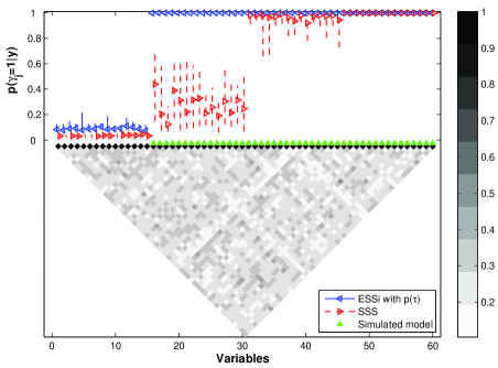
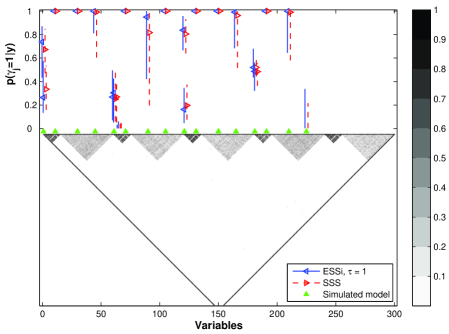
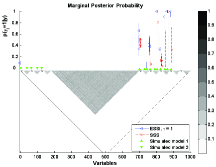
Figure 6 presents the marginal posterior probability of inclusion for ESS$i$ with $\tau=1$ averaged across replicates and, as a measure of variability, the interquartile range, blue left triangles and vertical blue solid line respectively. In general the covariates with non-zero effects have high marginal posterior probability of inclusion in all the examples: for example in Ex3, Figure 6 (a), the proposed ESS$i$ algorithm, blue left triangle, is able to perfectly select the last $45$ covariates, while the first $15$, which do not contribute to $y$, receive small marginal posterior probability. It is interesting to note that this group of covariates, $\left(\beta_{1},\ldots,\beta_{15}\right)=\left(0,\ldots,0\right)$, although correctly recognised having no influence on $y$, show some variability across replicates, vertical blue solid line: however, this is not surprising since independent priors are less suitable in situations where all the covariates are mildly-strongly correlated as in this simulated example. On the other hand the second set of covariates with small effects, $\left(\beta_{16},\ldots,\beta_{30}\right)=\left(1,\ldots,1\right)$, are univocally detected. The ability of ESS$i$ to select variables with small effects is also evident in Ex6, Figure 6 (d), where the two smallest coefficients, $\beta_{2}=0.112$ and $\beta_{10}=0.950$ (the second and last respectively from left to right), receive from high to very high marginal posterior probability (and similarly for the other replicates, data not shown). In some cases however, some covariates attached with small effects are missed (e.g. Ex4, Figure 6 (b), the last simulated effect which is also the smallest, $\beta_{16}=0.5$, is not detected). In this situation however the vertical blue solid line indicates that for some replicates, ESS$i$ is able to assign small values of the marginal posterior probability giving evidence that ESS$i$ fully explore the whole space of models.

Superimposed on all pictures of Figure 5 are the median and interquartile range across replicates of $p\left(\gamma_{j}=1\left|y\right.\right)$, $j=1,\ldots,p$, for SSS, red right triangles and vertical red dashed line respectively. We see that there is good agreement between the two algorithms in general, with in addition evidence that ESS$i$ is able to explore more fully the model space and in particular to find small effects, leading to a posterior model size that is close to the true one. For instance in Ex3, Figure 6 (a), where the last $30$ covariates accounts for most of $R_{\gamma}^{2}$, SSS has difficulty to detect $\left(\beta_{16},\ldots,\beta_{30}\right)$, while in Ex6, it misses $\beta_{2}=0.112$, the smallest effect, and surprisingly also $\beta_{4}=-2.595$ assigning a very small marginal posterior probability (and in general for the small effects in most replicates, data not shown). However the most marked difference between ESS$i$ and SSS is present in Ex5: as for ESS$i$, SSS misses three effects of “model 1”  but in addition $\beta_{4}=1$, $\beta_{7}=-1$ and $\beta_{8}=1.5$ receive also very low marginal posterior probability, red right triangle, with high variability across replicates, vertical red dashed line. Moreover on the extreme left, as noted before, ESS$i$ is able to capture the biggest coefficient of “model 2”  while SSS misses completely all contaminated effects. No noticeable differences between ESS$i$ and SSS are present in Ex1 and Ex2 for the marginal posterior probability, while in Ex4, SSS shows more variability in $p\left(\gamma_{j}=1\left|y\right.\right)$ (red dashed vertical lines compared to blue solid vertical lines) for some covariates that do receive the highest marginal posterior probability.

In contrast to the differences in the marginal posterior probability of inclusion, there is general agreement between the two algorithms with respect to some measures of goodness of fit and stability, see Table 6. Again, not surprisingly, the main difference is seen in Ex5 where ESS$i$ with $\tau=1$ reaches a better $R_{\gamma}^{2}$ both for the maximum and the $1,000$ largest $p\left(\gamma\left|y\right.\right)$. SSS shows more stability in all examples, but the last: this was somehow expected since one key features of SSS in its ability to move quickly towards the right model and to persist on it (Hans et al., 2007), but a drawback of this is its difficulty to explore far apart models with competing $R_{\gamma}^{2}$ as in Ex5. Note that ESS$i$ shows a small improvement of $R_{\gamma}^{2}$ in all the simulated examples. This is related to the ability of ESS$i$ to pick up some of the small effects that are missed by SSS, see Figure 6. Finally ESS$i$ shows a remarkable superiority in terms of computational time especially when the simulated (and estimated) $p_{\gamma}$ is large (in other simulated examples, data not shown, we found this is always true when $p_{\gamma}\gtrsim 10$): the explanation lies in the number of different models SSS and ESS$i$ evaluate at each sweep. Indeed, SSS evaluates $p+p_{\gamma}\left(p-p_{\gamma}\right)$, where $p_{\gamma}$ is the size of the current model, while ESS$i$ theoretically analyses an equally large number of models, $pL$, but, when $p>n$, the actual number of models evaluated is drastically reduced thanks to our FSMH sampler. In only one case SSS beats ESS$i$ in term of computational time (Ex5), but in this instance SSS clearly underestimates the simulated model and hence performs less evaluations than would be necessary to explore faithfully the model space. In conclusion, we see that the rich porfolio of moves and the use of parallel chains makes ESS robust for tackling complex covariate space as well as competitive against a state of the art search algorithm.

References

Abramowitz, M. and Stegun, I. (1970). Handbook of Mathematical Functions. New York: Dover Publications, Inc.

Altshuler, D., Brooks, L.D., Chakravarti, A., Collins, F.S., Daly, M.D. and Donnelly, P. (2005). A haplotype map of the human genome. Nature, 437, 1299-1320.

Bae, N. and Mallick, B.K. (2004). Gene selection using a two-level hierarchical Bayesian model. Bioinformatics, 20, 3423-3430.

Brown, P.J., Vannucci, M. and Fearn, T. (1998). Multivariate Bayesian variable selection and prediction. J. R. Statist. Soc. B, 60, 627-641.

Calvo, F. (2005) All-exchange parallel tempering. J. Chem. Phys., 123, 1-7.

Chipman, H. (1996). Bayesian variable selection with related predictors. Canad. J. Statist., 24, 17-36.

Chipman, H., George, E.I. and McCulloch, R.E. (2001). The practical implementation of Bayesian model selection (with discussion). In Model Selection (P. Lahiri, ed), 66-134. IMS: Beachwood, OH.

Clyde, M. and George, E. I. (2004). Model uncertainty. Statist. Sci., 19, 81-94.

Cui, W. and George, E.I. (2008). Empirical Bayes vs fully Bayes variable selection. J. Stat. Plan. Inf., 138, 888-900.

Dellaportas, P., Forster, J. and Ntzoufras, I. (2002). On Bayesian model and variable selection using MCMC. Statist. Comp., 12, 27-36.

Fernández, C., Ley, E. and Steel, M.F.J. (2001). Benchmark priors for Bayesian model averaging. J. Econometrics, 75, 317-343.

George, E.I. and McCulloch, R.E. (1993). Variable selection via Gibbs sampling. J. Am. Statist. Assoc., 88, 881-889.

George, E.I. and McCulloch, R.E. (1997). Approaches for Bayesian variable selection. Stat. Sinica, 7, 339-373.

Geweke, J. (1996). Variable selection and model comparison in regression. In Bayesian Statistics 5, Proc. 5th Int. Meeting (J.M. Bernardo, J.O. Berger, A.P. Dawid and A.F.M. Smith, eds), 609-20. Claredon Press: Oxford, UK.

Goswami, G. and Liu, J.S. (2007). On learning strategies for evolutionary Monte Carlo. Statist. Comp., 17, 23-38.

Gramacy, R.B, J. Samworth, R.J. and King, R. (2007). Importance Tempering. Tech. rep. Available at: http://arxiv.org/abs/0707.4242

Green, P. and Mira, A. (2001). Delayed rejection in reversible jump Metropolis-Hastings. Biometrika, 88, 1035-1053.

Iba, Y. (2001). Extended Ensemble Monte Carlo. Int. J. Mod. Phys., C, 12, 623-656.

Hans, C., Dobra, A. and West, M. (2007). Shotgun Stochastic Search for “large $p$” regression. J. Am. Statist. Assoc., 102, 507-517.

Hubner, N. et al. (2005). Integrated transcriptional profiling and linkage analysis for identification of genes underlying disease. Nat. Genet., 37, 243-253.

Kohn, R., Smith, M. and Chan, D. (2001). Nonparametric regression using linear combinations of basis functions. Statist. Comp., 11, 313-322.

Jasra, A., Stephens, D.A. and Holmes, C. (2007). Population-based reversible jump Markov chain Monte Carlo. Biometrika, 94, 787-807.

Liang, F., Paulo, R., Molina, G., Clyde, M.A. and Berger, J.O. (2008). Mixtures of $g$-priors for Bayesian variable selection. J. Am. Statist. Assoc., 481, 410-423.

Liang, F. and Wong, W.H. (2000). Evolutionary Monte Carlo: application to $C_{p}$ model sampling and change point problem. Stat. Sinica, 10, 317-342.

Liu, J.S. (2001). Monte Carlo strategies in scientific computations. Springer: New York.

Madigan, D. and York, J. (1995). Bayesian graphical models for discrete data. Int. Statist. Rev., 63, 215-232.

Natarajan, R. and McCulloch. (1998). Gibbs sampling with diffuse proper priors: a valid approach to data-driven inference?, J. Comp. Graph. Statist., 7, 267-277.

Nott, D.J. and Green, P.J. (2004). Bayesian variable selection and the Swedsen-Wang algorithm. J. Comp. Graph. Statist., 13, 141-157.

Roberts, G.O. and Rosenthal, J.S. (2008). Example of adaptive MCMC. Tech. rep. Available at: http://www.probability.ca/jeff/research.html

Tierney, L. and Kadane, J.B. (1986). Accurate approximations for posterior moments and marginal densities. J. Am. Statist. Assoc., 81, 82-86.

Wilson, M.A., Iversen, E.S., Clyde, M.A., Schmidler, S.C. and Shildkraut, J.M. (2009). Bayesian model search and multilevel inference for SNP association studies. Tech. rep. Available at:
http://arxiv.org/abs/0908.1144

Zellner, A. (1986). On assessing prior distributions and Bayesian regression analysis with $g$-prior distributions. In Bayesian Inference and Decision Techniques-Essays in Honour of Bruno de Finetti (P.K. Goel and A. Zellner, eds), 233-243. Amsterdam: North-Holland.

Zellner, A. and Siow, A. (1980). Posterior odds ratios for selected regression hypotheses. In Bayesian Statistics, Proc. 1st Int. Meeting (J.M. Bernardo, M.H. De Groot, D.V. Lindley and A.F.M. Smith, eds), 585-603. Valencia: University Press.

Figure 1: Top panels: (a) trace plot of the log posterior probability, $\log p\left(\gamma\left|y\right.\right)$, and (b) model size, $p_{\gamma}$, across sweeps for the first real data example, eQTL analysis, using ESS$g$ with $\tau=29$ and FSMH as local move. Vertical dashed lines indicate the end of the burn-in. Bottom panels: (c) trace plot of the log posterior probability when MC₃ is used as a local move; (d) kernel densities of $\log p\left(\gamma\left|y\right.\right)$ for the retained chain in the 25 replicates of the analysis when only FSMH and only MC₃ are used as a local move respectively. Plot restricted to regions of high posterior probability.

Figure 2: (a) Posterior model size for the first real data example, eQTL analysis: black solid line for ESS$g$ with $\tau$ fixed at $29$ and black dashed line for ESS$g$ with Z-S prior. (b) Posterior model size for mQTL analysis, second real data example, using ESS$g$ with fixed and random $\tau$.

Figure 3: Trace plot of the proposal’s standard deviation for $\tau$ for the two real data examples analysed using ESS$g$ with Z-S prior. Vertical dashed lines indicate the end of the burn-in.

Figure 4: Accumulated posterior mass as a function of the models recorded. Plot generated using $25$ replicates of the analysis of the first real data example and normalised by the total mass found by ESS$g$, $\tau=29$, with only block crossover move ($\rho_{0}=0.25$). 1-point and uniform crossover accumulate around $90$% of the total mass accumulated by ESS$g$ with only block crossover, while adaptive crossover only $85$%.

Figure 5: For ESS$i$ with $\tau=1$: (a) trace plot of the log posterior probability, $\log p\left(\gamma\left|y\right.\right)$, and (b) model size, $p_{\gamma}$, across sweeps for one replicate of Ex1 with $E\left(p_{\gamma}\right)=20$, top panels and Ex4, bottom panels. Vertical dashed lines indicate the end of the burn-in.

Figure 6: Median and interquartile range of the marginal posterior probability of inclusion (A.12) for Ex3, (a), Ex4, (b) and Ex5, (c), across replicates. Each graph is constructed as follows: bottom part, pairwise squared correlation $\rho^{2}\left(X_{j},X_{j^{\prime}}\right)$, $j=1,\ldots,p$, between predictors for one selected replicate, grey scale indicates different values of squared correlation; blue left and red right triangles, median of $p\left(\gamma_{j}=1\left|y\right.\right)$ across replicates for ESS$i$ with $\tau=1$ and SSS respectively; vertical blue solid lines and vertical red dashed lines, interquartile range of $p\left(\gamma_{j}=1\left|y\right.\right)$ across replicates for ESS$i$ and SSS respectively; upper and lower green triangles, simulated models. Selected replicate of Ex6, (d), shows marginal posterior probability of inclusion (blue left and red right triangles for ESS$i$ $\tau=1$ and SSS respectively). Marginal posterior probability of inclusion lower than $0.025$ not shown.

Mode$\left(p_{\gamma}\left|y\right.\right)$ $E\left(\tau\left|y\right.\right)$ $\left.R_{\gamma}^{2}\right.^{\ast}$ $\left.\overline{R_{\gamma}^{2}}\right.^{\ast\ast}$ Stability eQTL ESS$g$, $\tau=29$ $2$ $-$ $0.716$ $0.704$ $0.257$ ESS$g$ with $p\left(\tau\right)$ $2$ $20.576$ $0.716$ $0.689$ $0.099$ mQTL ESS$g$, $\tau=50$ $2$ $-$ $0.843$ $0.843$ $\approx 0$ ESS$g$ with $p\left(\tau\right)$ $2$ $63.577$ $0.843$ $0.843$ $\approx 0$ Crossover DR Exchange ALL Exchange $\text{Acc. rate }\tau$ Time (min.) eQTL ESS$g$, $\tau=29$ $0.214$ $0.534$ $0.671$ $-$ $28$ ESS$g$ with $p\left(\tau\right)$ $0.243$ $0.585$ $0.711$ $0.438$ $30$ mQTL ESS$g$, $\tau=50$ $0.214$ $0.514$ $0.669$ $-$ $302$ ESS$g$ with $p\left(\tau\right)$ $0.226$ $0.571$ $0.717$ $0.434$ $309$

Table 1: Performance of ESS$g$ with and without the hyperprior on $\tau$ for the first real data example, eQTL analysis, and second example, mQTL analysis. $\left.R_{\gamma}^{2}\right.^{\ast}$ and $\left.\overline{R_{\gamma}^{2}}\right.^{\ast\ast}$ correspond to “$R_{\gamma}^{2}$: $\max p\left(\gamma\left|y\right.\right)$” and “$\overline{R_{\gamma}^{2}}$: $1,000$ largest $p\left(\gamma\left|y\right.\right)$” respectively. The former indicates the coefficient of determination for the (first chain) best model visited according to the posterior probability $p\left(\gamma\left|y\right.\right)$, while the latter shows the average $R_{\gamma}^{2}$ for the (first chain) top $1,000$ (not unique) visited models ranked by the posterior probability. “Stability” is defined as the standard deviation of $R_{\gamma}^{2}$ for the (first chain) top $1,000$ (not unique) visited models (smaller values indicate better performance of the algorithm). In the bottom part of the Table, acceptance rate for specific moves are given. “DR Exchange” and “ALL Exchange” stands for “delayed rejection exchange” and “all-exchange” move respectively.

Version of ESS$g$ $\tau$ $p\left(\tau\right)$ Experiment (i) ESS$g$ with only FSMH $68\%$ $88\%$ ESS$g$ with only MC³ $28\%$ $40\%$ Experiment (ii) ESS$g$ with only 1-point crossover $64\%$ $80\%$ ESS$g$ with only block crossover $80\%$ $84\%$ ESS$g$ with only uniform crossover $60\%$ $84\%$ ESS$g$ with only adaptive crossover $60\%$ $76\%$

Table 2: Proportion of times different versions of ESS$g$ reach the same top visited model in the eQTL real data set with or without an hyperprior on $\tau$ in $25$ replicates of the analysis.

Version of ESS$g$ $\tau$ $p\left(\tau\right)$ Experiment (ii) ESS$g$ with only 1-point crossover $0.303$ $0.335$ ESS$g$ with only block crossover $0.482$ $0.501$ ESS$g$ with only uniform crossover $0.026$ $0.042$ ESS$g$ with only adaptive crossover $0$ $0.013$

Table 3: Average acceptance rate of the crossover operator for different versions of ESS$g$ in $25$ replicates of the analysis of the first real data example with or without an hyperprior on $\tau$.

Ex1 Ex2 Ex3 Ex4 Ex5 Ex6 $\begin{array}[]{c}{\small n}\\ {\small p}\end{array}$ $120$ $300$ $120$ $120$ $200$ $120$ $60$ $30$ $60$ $300$ $1,000$ $775$ $E\left(p_{\gamma}\right)$ $5$ $10$ $20$ $5$ $5$ $5$ $5$ $5$ Add/delete $0.036$ $0.054$ $0.098$ $0.066$ $0.086$ - - - $\left(0.016\right)$ $\left(0.017\right)$ $\left(0.023\right)$ $\left(0.020\right)$ $\left(0.031\right)$ - - - Swap $0.063$ $0.100$ $0.165$ $0.070$ $0.106$ - - - $\left(0.015\right)$ $\left(0.019\right)$ $\left(0.022\right)$ $\left(0.015\right)$ $\left(0.053\right)$ - - - Crossover $0.249$ $0.270$ $0.271$ $0.157$ $0.215$ $0.147$ $0.170$ $0.193$ $\left(0.021\right)$ $\left(0.029\right)$ $\left(0.036\right)$ $\left(0.018\right)$ $\left(0.022\right)$ $\left(0.028\right)$ $\left(0.023\right)$ $\left(0.028\right)$ DR Exchange $0.500$ $0.493$ $0.500$ $0.582$ $0.492$ $0.517$ $0.505$ $0.497$ $\left(0.040\right)$ $\left(0.043\right)$ $\left(0.040\right)$ $\left(0.020\right)$ $\left(0.071\right)$ $\left(0.105\right)$ $\left(0.013\right)$ $\left(0.072\right)$

Table 4: Mean and standard deviation in brackets of EMC acceptance rates across replicates for ESS$i$ with $\tau=1$. “DR Exchange” stands for “delayed rejection exchange”.

Ex1 Ex2 Ex3 Ex4 Ex5 Ex6 $\begin{array}[]{c}{\small n}\\ {\small p}\end{array}$ $120$ $300$ $120$ $120$ $200$ $120$ $60$ $30$ $60$ $300$ $1,000$ $775$ $E\left(p_{\gamma}\right)$ $5$ $10$ $20$ $5$ $5$ $5$ $5$ $5$ Swapping $\begin{array}[]{c}l=1\\ l=2\\ l=3\\ l=4\\ l=5\end{array}$ $\begin{array}[]{c}0.157\\ 0.250\\ 0.220\\ 0.240\\ 0.142\end{array}$ $\begin{array}[]{c}0.137\\ 0.232\\ 0.220\\ 0.252\\ 0.160\end{array}$ $\begin{array}[]{c}0.110\\ 0.204\\ 0.223\\ 0.280\\ 0.182\end{array}$ $\begin{array}[]{c}0.065\\ 0.185\\ 0.255\\ 0.293\\ 0.201\end{array}$ $\begin{array}[]{c}0.160\\ 0.271\\ 0.245\\ 0.215\\ 0.110\end{array}$ $\begin{array}[]{c}0.180\\ 0.276\\ 0.223\\ 0.206\\ 0.112\end{array}$ $\begin{array}[]{c}0.201\\ 0.300\\ 0.231\\ 0.182\\ 0.083\end{array}$ $\begin{array}[]{c}0.214\\ 0.316\\ 0.231\\ 0.167\\ 0.070\end{array}$ Overlapping $\begin{array}[]{c}l=1,2\\ l=2,3\\ l=3,4\\ l=4,5\end{array}$ $\begin{array}[]{c}1.360\\ 1.570\\ 1.400\\ 1.100\end{array}$ $\begin{array}[]{c}1.600\\ 1.570\\ 1.290\\ 0.992\end{array}$ $\begin{array}[]{c}2.101\\ 1.600\\ 1.050\\ 0.690\end{array}$ $\begin{array}[]{c}2.680\\ 0.870\\ 0.600\\ 1.251\end{array}$ $\begin{array}[]{c}1.350\\ 1.430\\ 2.111\\ 4.131\end{array}$ $\begin{array}[]{c}0.733\\ 1.021\\ 1.329\\ 1.503\end{array}$ $\begin{array}[]{c}0.569\\ 0.913\\ 1.491\\ 2.304\end{array}$ $\begin{array}[]{c}0.526\\ 0.893\\ 1.696\\ 2.499\end{array}$

Table 5: Swapping probability for ESS$i$ with $\tau=1$ defined as the observed frequency of successful swaps for each chain (including delayed rejection exchange and all-exchange operators) averaged across replicates. Overlapping measure defined as $V\left(f\left(\gamma_{l}\right)\right)\left(1/t_{l+1}-1/t_{l}\right)^{2}$, Liang and Wong (2000) with $f\left(\gamma_{l}\right)=\log p\left(y\left|\gamma_{l}\right.\right)+\log p\left(\gamma_{l}\right)$. Target value for consecutive chains is $O\left(1\right)$.

Ex1 Ex2 Ex3 Ex4 Ex5 Ex6 $\begin{array}[]{c}{\small n}\\ {\small p}\end{array}$ $120$ $300$ $120$ $120$ $200$ $120$ $60$ $30$ $60$ $300$ $1,000$ $775$ $E\left(p_{\gamma}\right)$ $5$ $10$ $20$ $5$ $5$ $5$ $5$ $5$ $\begin{array}[]{c}\text{ESS}i,\\ \tau\text{=1}\end{array}$ $\left.R_{\gamma}^{2}\right.^{\ast}$      $0.864$ $0.867$ $0.871$ $0.975$ $\approx 1$ $0.962$ $0.703$ $0.997$ $\left(0.029\right)$ $\left(0.027\right)$ $\left(0.023\right)$ $\left(0.003\right)$ $\left(\approx 0\right)$ $\left(0.011\right)$ $\left(0.043\right)$ $\left(0.005\right)$ $\left.\overline{R_{\gamma}^{2}}\right.^{\ast\ast}$      $0.863$ $0.866$ $0.874$ $0.975$ $\approx 1$ $0.957$ $0.689$ $0.997$ $\left(0.027\right)$ $\left(0.026\right)$ $\left(0.023\right)$ $\left(0.003\right)$ $\left(\approx 0\right)$ $\left(0.014\right)$ $\left(0.048\right)$ $\left(0.003\right)$ Stability      $0.003$ $0.003$ $0.005$ $\approx 0$ $\left(\approx 0\right)$ $0.005$ $0.015$ $0.002$ $\left(0.001\right)$ $\left(0.002\right)$ $\left(0.002\right)$ $\left(\approx 0\right)$ $\left(\approx 0\right)$ $\left(0.004\right)$ $\left(0.007\right)$ $\left(0.002\right)$ Time (min.)      $6$ $6$ $7$ $16$ $18$ $166$ $338$ $202$ $\left(<1\right)$ $\left(<1\right)$ $\left(<1\right)$ $\left(<1\right)$ $\left(1\right)$ $\left(32\right)$ $\left(43\right)$ $\left(40\right)$ SSS $\left.R_{\gamma}^{2}\right.^{\ast}$      $0.863$ $0.867$ $0.870$ $0.975$ $\approx 1$ $0.956$ $0.577$ $0.997$ $\left(0.027\right)$ $\left(0.025\right)$ $\left(0.024\right)$ $\left(0.003\right)$ $\left(\approx 0\right)$ $\left(0.016\right)$ $\left(0.074\right)$ $\left(0.004\right)$ $\left.\overline{R_{\gamma}^{2}}\right.^{\ast\ast}$      $0.863$ $0.867$ $0.870$ $0.975$ $0.999$ $0.955$ $0.565$ $0.996$ $\left(0.027\right)$ $\left(0.025\right)$ $\left(0.024\right)$ $\left(0.003\right)$ $\left(\approx 0\right)$ $\left(0.016\right)$ $\left(0.078\right)$ $\left(0.004\right)$ Stability      $0$ $0$ $\approx 0$ $\approx 0$ $\approx 0$ $0.001$ $0.009$ $0.004$ $\left(0\right)$ $\left(0\right)$ $\left(\approx 0\right)$ $\left(\approx 0\right)$ $\left(\approx 0\right)$ $\left(0.002\right)$ $\left(0.015\right)$ $\left(0.006\right)$ Time (min.)      $12$ $12$ $13$ $118$ $497$ $502$ $169$ $549$ $\left(1\right)$ $\left(2\right)$ $\left(2\right)$ $\left(26\right)$ $\left(75\right)$ $\left(241\right)$ $\left(81\right)$ $\left(159\right)$

Table 6: Comparison between ESS$i$ with $\tau=1$ and SSS for the six simulated examples. Standard deviation in brackets. $\left.R_{\gamma}^{2}\right.^{\ast}$ and $\left.\overline{R_{\gamma}^{2}}\right.^{\ast\ast}$ correspond to “$R_{\gamma}^{2}$: $\max p\left(\gamma\left|y\right.\right)$” and “$\overline{R_{\gamma}^{2}}$: $1,000$ largest $p\left(\gamma\left|y\right.\right)$” respectively.