Radiative contribution to neutrino masses and mixing in μν𝜇𝜈\mu\nuSSM

Pradipta Ghosh,a  Paramita Dey,b  Biswarup Mukhopadhyayaa,c and Sourov Roya
aDepartment of Theoretical Physics and Centre for Theoretical Sciences,
Indian Association for the Cultivation of Science,
2A &\& 2B Raja S.C. Mullick Road, Kolkata 700 032, India
bInstitut fu¨¨𝑢\ddot{u}r Theoretische Teilchenphysik und Kosmologie,
RWTH Aachen University,
D-52056 Aachen, Germany
cRegional Centre for Accelerator-based Particle Physics,
Harish-Chandra Research Institute,
Chhatnag Road, Jhusi, Allahabad–211019, India
E-mails
tppg@iacs.res.in, paramita@physik.rwth-aachen.de, biswarup@mri.ernet.in, tpsr@iacs.res.in
Abstract:

In an extension of the minimal supersymmetric standard model (popularly known as the μν𝜇𝜈\mu\nuSSM), three right handed neutrino superfields are introduced to solve the μ𝜇\mu-problem and to accommodate the non-vanishing neutrino masses and mixing. Neutrino masses at the tree level are generated through Rlimit-from𝑅R-parity violation and seesaw mechanism. We have analyzed the full effect of one-loop contributions to the neutrino mass matrix. We show that the current three flavour global neutrino data can be accommodated in the μν𝜇𝜈\mu\nuSSM, for both the tree level and one-loop corrected analyses. We find that it is relatively easier to accommodate the normal hierarchical mass pattern compared to the inverted hierarchical or quasi-degenerate case, when one-loop corrections are included.

Beyond Standard Model, Neutrino Physics, Supersymmetric Standard Model
preprint: TTK-10-17
HRI-RECAPP-2010-003

1 Introduction

Despite its stupendous success in explaining elementary particle interactions, the celebrated standard model (SM) of particle physics suffers from some shortcomings, both theoretical and experimental. On the experimental side, explaining the masses and the mixing pattern of neutrinos is a task in which the SM is an apparent failure. The neutrino sector, therefore, is a natural testing ground for most proposals for going beyond the SM.

Supersymmetry (SUSY) is a rather popular choice for new physics. The minimal supersymmetric version of the SM (MSSM) provides a natural solution to the so-called “gauge-hierarchy problem” through the introduction of superpartners of SM-particles. However, MSSM itself is not free of drawbacks. One of these is the so-called μ𝜇\mu-problem [1], which essentially means our lack of understanding as to why the higgsino mass parameter, a SUSY invariant quantity, has to be around the SUSY breaking scale. This problem can be solved in the next-to minimal supersymmetric version of the standard model (NMSSM), where, unlike in the MSSM, the μ𝜇\mu-term becomes a derived quantity with the right order of magnitude.

Unfortunately, neither the MSSM nor NMSSM by itself can explain the observed pattern of neutrino masses and mixing, on which definite guidelines have been set down by existing data [2, 3]. The situation becomes different if one allows violation of the discrete symmetry known as R𝑅R-parity (Rpsubscript𝑅𝑝R_{p}) [4, 5, 6, 7, 8, 9, 10, 11, 12], defined as Rp=(1)L+3B+2Ssubscript𝑅𝑝superscript1𝐿3𝐵2𝑆R_{p}=(-1)^{L+3B+2S}, where L(B)𝐿𝐵L(B) is the lepton(baryon) number and S𝑆S is the spin, of a particle. Neutrino masses and mixing have been analyzed in these models under various assumptions, both at the tree level and by taking loop-induced effects into account. Neutrino mass generation in variants of Rpsubscript𝑅𝑝R_{p} violating MSSM have been addressed in refs. [13, 14, 15, 16, 18, 17, 19, 20, 21, 22, 23, 24, 25, 26, 27, 28, 29, 30, 31, 32, 33, 34, 35, 36, 37, 38, 39, 40, 41, 42, 43, 44, 45, 46, 47, 48, 49, 50, 51, 52, 53, 54, 55, 56, 57, 58, 59, 60, 61, 62]. Such extensive study has established Rpsubscript𝑅𝑝R_{p}-violation to be as potent in neutrino mass generation as the well-known seesaw mechanism [63, 64, 65, 66, 67] which requires introduction of gauge singlet neutrino superfields.

R-parity violation, in both the contexts of accelerator phenomenology and, for example, neutrino mass generation, have been extensively studied in various scenarios, especially in its L-violating incarnation. Thus one has so-called trilinear R-parity violation driven by the λijksubscript𝜆𝑖𝑗𝑘\lambda_{ijk} or λijksubscriptsuperscript𝜆𝑖𝑗𝑘\lambda^{\prime}_{ijk}-type terms in the superpotential. In addition to new signals induced by three-body decays of the lightest neutralino, neutrino masses are generated through loop effects in such scenarios [13, 14, 15, 16, 18, 17, 19, 20]. Then one can have R-parity broken by bilinear terms [21, 22, 23, 24, 25, 26, 27, 28, 29, 30, 31, 32, 33, 34, 35, 36, 37, 38, 39, 40, 41, 42, 43, 44, 45, 46, 47, 48, 49, 50, 51, 52, 53, 54, 55, 56, 57, 58] of the type ϵiLiH2subscriptitalic-ϵ𝑖subscript𝐿𝑖subscript𝐻2\epsilon_{i}L_{i}H_{2}. One here notices remarkable features like (a) non-zero vacuum expectation values for sneutrinos, and (b) the mixing between neutrinos and neutralinos as well as charged leptons and charginos. Such a scenario generates one neutrino mass at the tree level while the other mass(es) need to be generated via loop effects [39, 40, 41, 42, 43, 44, 45, 46, 47, 48, 49, 50, 51]. The characteristic signal consists in final state with comparable numbers of muons and taus at high energy colliders [52, 53, 54, 55, 56, 57, 58].

Bilinear R-parity violation, is also linked with spontaneous L-breaking [10, 59, 60, 61, 62] via a singlet sneutrino vacuum expectation value (VEV). Such an effect triggers terms of the type ϵiLiH2subscriptitalic-ϵ𝑖subscript𝐿𝑖subscript𝐻2\epsilon_{i}L_{i}H_{2} in the superpotential, and also leaves as its footprint a Majoron which has its own experimental signature [68, 69, 70], being an additional source of missing energy.

In the backdrop of such a rich phenomenology of relatively minimalistic R-parity breaking models, further embellishments on the minimal scenarios have also been studied, often with some specific goals. A proposal for neutrino mass generation together with a solution to the μ𝜇\mu-problem, with the same set of gauge-singlet right chiral neutrino superfields, has been advocated in [71]. This is popularly known as μν𝜇𝜈\mu\nuSSM. Following this proposal, the scalar sector and the parameter space of μν𝜇𝜈\mu\nuSSM was studied in great detail in [72]. In μν𝜇𝜈\mu\nuSSM, the three generations of SM-neutrinos can acquire masses through a TeV-scale seesaw mechanism, with both neutralinos and heavy neutrinos participating in the process [73]. Issues of neutrino mass generation and the μ𝜇\mu-problem can also be found in some recent works [74, 75, 76, 77, 78].

A comprehensive analytical study of mass generation of light neutrinos in μν𝜇𝜈\mu\nuSSM, accompanied by necessary numerical analysis, has been discussed in ref. [73]. In this work, neutrino masses and mixing, consistent with the three flavour global neutrino data, are reproduced even with the simplistic choice of flavour diagonal neutrino Yukawa couplings (Yνii)subscriptsuperscript𝑌𝑖𝑖𝜈(Y^{ii}_{\nu}). Decay modes of the lightest neutralino into two-body final states (Z0νsuperscript𝑍0subscript𝜈Z^{0}\nu_{\ell}W±superscript𝑊plus-or-minusW^{\pm}\ell) have also been considered for various compositions of the lightest neutralino. In addition, correlations between neutrino mixing angles, and ratio of the decay branching ratios into W±superscript𝑊plus-or-minusW^{\pm}-charged lepton are studied there as a possible test of this model at the Large Hadron Collider (LHC).

Among other related studies of importance, neutrino mass generation and collider aspects of this model, with one and two generation(s) of the right handed neutrinos, have been addressed in ref.[79]. For one right handed neutrino, neutrino mass generation has been studied there upto one-loop level. Decays of the lightest neutralino into all possible final states are also studied in this reference. Constraints on complex vacuum expectation values (VEVs) from electroweak symmetry breaking (EWSB), and its consequence on the neutrino sector are studied in ref.[80], where issues concerning spontaneous CP-violation are also addressed. The role of gravitino as a dark matter candidate in this model was studied in ref.[81]. This paper also highlighted the prospects of detecting gamma rays from decaying gravitinos. For an overview of various other aspects of μν𝜇𝜈\mu\nuSSM, see the recent review [82].

In this work, we study in detail the effect of radiative corrections, upto one-loop, to the neutrino masses and mixing, consistent with the three flavour global data [2, 3]. As mentioned before, a similar study, but with just one generation of right handed neutrino, was carried out in [79]. However, a full study addressing both neutrino masses and the bilarge mixing pattern, with a complete set of one-loop corrections with all three generations of left and right handed neutrinos, has so far been lacking. This is exactly what we attempt in the present work. We also perform a systematic study to identify the crucial parameters of the model, which control the tree level or the one-loop dominance in the neutrino sector.

As shown in Ref.[73, 79], a very attractive feature of this model is that the ratios of certain decay branching ratios show very nice correlation with the neutrino mixing angles. This is very similar to bilinear R-parity violating models [52, 53, 56]. Nevertheless, one should note certain differences in these two cases. In μν𝜇𝜈\mu\nuSSM lepton number is broken explicitly in the superpotential by terms which are trilinear as well as linear in singlet neutrino superfields. In addition to that there are lepton number conserving terms involving the singlet neutrino superfields with dimensionless neutrino Yukawa couplings. After the electroweak symmetry breaking these terms can generate the effective bilinear R-parity violating terms as well as the ΔLΔ𝐿\Delta L =2 Majorana mass terms for the singlet neutrinos in the superpotential. In general, there are corresponding soft supersymmetry breaking terms in the scalar potential. Thus the parameter space of this model is much larger compared to the bilinear R-parity violating model. Hence, in general, one would not expect a very tight correlation between the neutrino mixing angles and the ratios of decay branching ratios of the LSP. However, under certain simplifying assumptions (as discussed in Sec. 3.2), one can reduce the number of free parameters and in those cases it is possible that the above correlations reappear. As mentioned earlier, this has been studied in great detail for the two body W𝑊\ell-W final states in [73] and for all possible two and three body final states in [79]. Let us note in passing that such a nice correlation is lost in the general scenario of bilinear-plus-trilinear R-parity violation [53].

Another important difference between μν𝜇𝜈\mu\nuSSM and the bilinear R-parity violating model in the context of the decay of the LSP (assumed to be the lightest neutralino in this case) is that in μν𝜇𝜈\mu\nuSSM the lightest neutralino can have a significant singlet neutrino (νcsuperscript𝜈𝑐\nu^{c}) contribution. In this case, the correlation between neutrino mixing angles and decay branching ratios of the LSP is different [73, 79] compared to the cases when the dominant component of the LSP is either a bino, or a higgsino or a Wino. This gives us a possibility of distinguishing between different R-parity violating models through the observation of the decay branching ratios of the LSP in collider experiments [73, 79]. In addition, the decay of the lightest neutralino will show displaced vertices in collider experiments and when the lightest neutralino is predominantly a singlet neutrino, the decay length can be of the order of several meters for a lightest neutralino mass in the neighbourhood of 50 GeV [79]. This is very different from the bilinear R-parity violating model where for a Bino LSP of similar mass the decay length is less than or of the order of a meter or so [56].

The paper is organized as follows. We start with a brief introduction to the model in section 2 and discuss the electroweak symmetry breaking conditions. The neutrino sector is discussed in section 3 in details, accompanied with necessary analytical results. We discuss the observed pattern of neutrino masses and mixing upto one-loop corrections. We present a comprehensive discussion on the results of our numerical analysis of neutrino masses and mixing in section 4. The three broad scenarios, namely, normal hierarchy, inverted hierarchy, and quasi-degenerate neutrinos, are taken up in turn in this section. We conclude in section 5. Various technical details, such as different mass matrices, couplings, Feynman rules and the expressions for one-loop contributions are relegated to the appendices.

2 Electroweak symmetry breaking in μν𝜇𝜈\mu\nuSSM

The superpotential for μν𝜇𝜈\mu\nuSSM includes three gauge-singlet right handed neutrino superfields (ν^icsuperscriptsubscript^𝜈𝑖𝑐{\hat{\nu}}_{i}^{c} (i=e,μ,τ𝑖𝑒𝜇𝜏i=e,{\mu},{\tau})) along with the usual MSSM superfields. The superpotential of μν𝜇𝜈\mu\nuSSM along the lines of ref.[71] is

W𝑊\displaystyle W =\displaystyle= ϵab(YuijH^2bQ^iau^jc+YdijH^1aQ^ibd^jc+YeijH^1aL^ibe^jc+YνijH^2bL^iaν^jc)subscriptitalic-ϵ𝑎𝑏subscriptsuperscript𝑌𝑖𝑗𝑢subscriptsuperscript^𝐻𝑏2subscriptsuperscript^𝑄𝑎𝑖subscriptsuperscript^𝑢𝑐𝑗subscriptsuperscript𝑌𝑖𝑗𝑑subscriptsuperscript^𝐻𝑎1subscriptsuperscript^𝑄𝑏𝑖subscriptsuperscript^𝑑𝑐𝑗subscriptsuperscript𝑌𝑖𝑗𝑒subscriptsuperscript^𝐻𝑎1subscriptsuperscript^𝐿𝑏𝑖subscriptsuperscript^𝑒𝑐𝑗subscriptsuperscript𝑌𝑖𝑗𝜈subscriptsuperscript^𝐻𝑏2subscriptsuperscript^𝐿𝑎𝑖subscriptsuperscript^𝜈𝑐𝑗\displaystyle\epsilon_{ab}(Y^{ij}_{u}\hat{H}^{b}_{2}\hat{Q}^{a}_{i}\hat{u}^{c}_{j}+Y^{ij}_{d}\hat{H}^{a}_{1}\hat{Q}^{b}_{i}\hat{d}^{c}_{j}+Y^{ij}_{e}\hat{H}^{a}_{1}\hat{L}^{b}_{i}\hat{e}^{c}_{j}+Y^{ij}_{\nu}\hat{H}^{b}_{2}\hat{L}^{a}_{i}\hat{\nu}^{c}_{j}) (1)
\displaystyle- ϵabλiν^icH^1aH^2b+13κijkν^icν^jcν^kc,subscriptitalic-ϵ𝑎𝑏superscript𝜆𝑖subscriptsuperscript^𝜈𝑐𝑖subscriptsuperscript^𝐻𝑎1subscriptsuperscript^𝐻𝑏213superscript𝜅𝑖𝑗𝑘subscriptsuperscript^𝜈𝑐𝑖subscriptsuperscript^𝜈𝑐𝑗subscriptsuperscript^𝜈𝑐𝑘\displaystyle\epsilon_{ab}\lambda^{i}\hat{\nu}^{c}_{i}\hat{H}^{a}_{1}\hat{H}^{b}_{2}+\frac{1}{3}\kappa^{ijk}\hat{\nu}^{c}_{i}\hat{\nu}^{c}_{j}\hat{\nu}^{c}_{k},

where H^1subscript^𝐻1\hat{H}_{1} and H^2subscript^𝐻2\hat{H}_{2} are the Higgs superfields that have Yukawa couplings with down- and up-type quarks, respectively. Q^isubscript^𝑄𝑖\hat{Q}_{i} are doublet quark superfields, u^jcsubscriptsuperscript^𝑢𝑐𝑗{\hat{u}}^{c}_{j} (d^jcsubscriptsuperscript^𝑑𝑐𝑗{\hat{d}}^{c}_{j}) are singlet up-type (down-type) quark superfields, L^isubscript^𝐿𝑖\hat{L}_{i} are doublet lepton superfields, and e^jcsubscriptsuperscript^𝑒𝑐𝑗{\hat{e}}^{c}_{j} are singlet charged lepton superfields. The absence of any bilinear terms in the superpotential is ensured by imposing a Z3subscript𝑍3Z_{3} symmetry (which is also used in case of NMSSM). The effective μ𝜇\mu-term is given by μ=λivic𝜇superscript𝜆𝑖subscriptsuperscript𝑣𝑐𝑖\mu=\sum{\lambda^{i}}{v^{c}_{i}}, where vicsubscriptsuperscript𝑣𝑐𝑖{v^{c}_{i}} is the VEV obtained by the ‘i𝑖i’-th right handed sneutrino (scalar component of ν^icsubscriptsuperscript^𝜈𝑐𝑖\hat{\nu}^{c}_{i}) after EWSB. The characteristic bilinear Rpsubscript𝑅𝑝R_{p} violating terms (εiL^iH^2subscript𝜀𝑖subscript^𝐿𝑖subscript^𝐻2\varepsilon_{i}{\hat{L}}_{i}{\hat{H}}_{2}) appear in a similar way after the EWSB. These terms are given by εi=Yνijvjcsuperscript𝜀𝑖subscriptsuperscript𝑌𝑖𝑗𝜈subscriptsuperscript𝑣𝑐𝑗\varepsilon^{i}=\sum Y^{ij}_{\nu}v^{c}_{j}. The last two terms of the superpotential (see eq.(1)) violate Rpsubscript𝑅𝑝R_{p} through L-violation. The last term, with the coefficient κijksuperscript𝜅𝑖𝑗𝑘\kappa^{ijk}, is included in order to avoid an unacceptable axion associated to the breaking of a global U(1)U1\rm U(1) symmetry [83]. This term generates effective Majorana masses for the singlet neutrinos at the electroweak scale.

It has been shown earlier [71, 72, 73] that the above RPsubscript𝑅𝑃R_{P}-violating superpotential (see eq.(1)) provides the minimal structure, sufficient for both generating a neutrino mass pattern, and offering a solution to the μ𝜇\mu-problem. There have been studies [84, 85] on RPsubscript𝑅𝑃R_{P}-violating scenarios including right handed neutrinos, which use a subset of this minimal superpotential, but without any attempt to address the μ𝜇\mu-problem. Similar remarks apply to earlier works [86] aimed at explaining the baryon asymmetry of the universe through leptogenesis, using the term ν^cH^1H^2superscript^𝜈𝑐subscript^𝐻1subscript^𝐻2{\hat{\nu}}^{c}{\hat{H}}_{1}{\hat{H}}_{2}.

The frequently discussed trilinear L𝐿L-violating terms, driven by the well-known λ𝜆\lambda- and λsuperscript𝜆\lambda^{\prime}-type couplings, need not appear explicitly in this model. The reason is the following; the above superpotential, as has already been stated, can lead to ‘bilinear’ terms of the form LiH2subscript𝐿𝑖subscript𝐻2L_{i}H_{2} once the right sneutrinos acquire VEV, and, once such terms arise, they can effectively lead to the λ𝜆\lambda and λsuperscript𝜆\lambda^{\prime}-type terms [30, 31]. Here, as a digression, let us mention that the spontaneous breakdown of the Z3subscript𝑍3Z_{3} symmetry through right-sneutrino VEV can in general lead to the formulation of domain walls [87]. The associated problems can, however, be ameliorated through well-known methods [88].

Coming back to μν𝜇𝜈\mu\nuSSM, if we confine ourselves to the framework of supergravity mediated supersymmetry breaking, the Lagrangian softsubscriptsoft\mathcal{L}_{\text{soft}}, containing the soft-supersymmetry-breaking terms is given by

softsubscriptsoft\displaystyle-\mathcal{L}_{\text{soft}} =\displaystyle= (mQ~2)ijQ~iaQja~+(mu~c2)iju~icu~jc+(md~c2)ijd~icd~jc+(mL~2)ijL~iaLja~superscriptsuperscriptsubscript𝑚~𝑄2𝑖𝑗subscriptsuperscript~𝑄superscript𝑎𝑖~subscriptsuperscript𝑄𝑎𝑗superscriptsuperscriptsubscript𝑚superscript~𝑢𝑐2𝑖𝑗subscriptsuperscript~𝑢superscript𝑐𝑖subscriptsuperscript~𝑢𝑐𝑗superscriptsuperscriptsubscript𝑚superscript~𝑑𝑐2𝑖𝑗subscriptsuperscript~𝑑superscript𝑐𝑖subscriptsuperscript~𝑑𝑐𝑗superscriptsuperscriptsubscript𝑚~𝐿2𝑖𝑗subscriptsuperscript~𝐿superscript𝑎𝑖~subscriptsuperscript𝐿𝑎𝑗\displaystyle(m_{\widetilde{Q}}^{2})^{ij}{\widetilde{Q}^{a^{*}}_{i}}\widetilde{Q^{a}_{j}}+(m_{\widetilde{u}^{c}}^{2})^{ij}{\widetilde{u}^{c^{*}}_{i}}\widetilde{u}^{c}_{j}+(m_{\widetilde{d}^{c}}^{2})^{ij}{\widetilde{d}^{c^{*}}_{i}}\widetilde{d}^{c}_{j}+(m_{\widetilde{L}}^{2})^{ij}{\widetilde{L}^{a^{*}}_{i}}\widetilde{L^{a}_{j}} (2)
+\displaystyle+ (me~c2)ije~ice~jc+mH12H1aH1a+mH22H2aH2a+(mν~c2)ijν~icν~jcsuperscriptsuperscriptsubscript𝑚superscript~𝑒𝑐2𝑖𝑗subscriptsuperscript~𝑒superscript𝑐𝑖subscriptsuperscript~𝑒𝑐𝑗superscriptsubscript𝑚subscript𝐻12subscriptsuperscript𝐻superscript𝑎1subscriptsuperscript𝐻𝑎1superscriptsubscript𝑚subscript𝐻22subscriptsuperscript𝐻superscript𝑎2subscriptsuperscript𝐻𝑎2superscriptsuperscriptsubscript𝑚superscript~𝜈𝑐2𝑖𝑗subscriptsuperscript~𝜈superscript𝑐𝑖subscriptsuperscript~𝜈𝑐𝑗\displaystyle(m_{\widetilde{e}^{c}}^{2})^{ij}{\widetilde{e}^{c^{*}}_{i}}\widetilde{e}^{c}_{j}+m_{H_{1}}^{2}{H^{a^{*}}_{1}}H^{a}_{1}+m_{H_{2}}^{2}{H^{a^{*}}_{2}}H^{a}_{2}+(m_{\widetilde{\nu}^{c}}^{2})^{ij}{\widetilde{\nu}^{c^{*}}_{i}}\widetilde{\nu}^{c}_{j}
+\displaystyle+ ϵab[(AuYu)ijH2bQ~iau~jc+(AdYd)ijH1aQ~ibd~jc+(AeYe)ijH1aL~ibe~jc+H.c.]subscriptitalic-ϵ𝑎𝑏delimited-[]superscriptsubscript𝐴𝑢subscript𝑌𝑢𝑖𝑗superscriptsubscript𝐻2𝑏subscriptsuperscript~𝑄𝑎𝑖superscriptsubscript~𝑢𝑗𝑐superscriptsubscript𝐴𝑑subscript𝑌𝑑𝑖𝑗superscriptsubscript𝐻1𝑎subscriptsuperscript~𝑄𝑏𝑖superscriptsubscript~𝑑𝑗𝑐superscriptsubscript𝐴𝑒subscript𝑌𝑒𝑖𝑗superscriptsubscript𝐻1𝑎subscriptsuperscript~𝐿𝑏𝑖superscriptsubscript~𝑒𝑗𝑐H.c.\displaystyle\epsilon_{ab}\left[(A_{u}Y_{u})^{ij}H_{2}^{b}\widetilde{Q}^{a}_{i}\widetilde{u}_{j}^{c}+(A_{d}Y_{d})^{ij}H_{1}^{a}\widetilde{Q}^{b}_{i}\widetilde{d}_{j}^{c}+(A_{e}Y_{e})^{ij}H_{1}^{a}\widetilde{L}^{b}_{i}\widetilde{e}_{j}^{c}+\text{H.c.}\right]
+\displaystyle+ [ϵab(AνYν)ijH2bL~iaν~jcϵab(Aλλ)iν~icH1aH2b+13(Aκκ)ijkν~icν~jcν~kc+H.c.]delimited-[]subscriptitalic-ϵ𝑎𝑏superscriptsubscript𝐴𝜈subscript𝑌𝜈𝑖𝑗superscriptsubscript𝐻2𝑏subscriptsuperscript~𝐿𝑎𝑖subscriptsuperscript~𝜈𝑐𝑗subscriptitalic-ϵ𝑎𝑏superscriptsubscript𝐴𝜆𝜆𝑖subscriptsuperscript~𝜈𝑐𝑖superscriptsubscript𝐻1𝑎superscriptsubscript𝐻2𝑏13superscriptsubscript𝐴𝜅𝜅𝑖𝑗𝑘subscriptsuperscript~𝜈𝑐𝑖subscriptsuperscript~𝜈𝑐𝑗subscriptsuperscript~𝜈𝑐𝑘H.c.\displaystyle\left[\epsilon_{ab}(A_{\nu}Y_{\nu})^{ij}H_{2}^{b}\widetilde{L}^{a}_{i}\widetilde{\nu}^{c}_{j}-\epsilon_{ab}(A_{\lambda}\lambda)^{i}\widetilde{\nu}^{c}_{i}H_{1}^{a}H_{2}^{b}+\frac{1}{3}(A_{\kappa}\kappa)^{ijk}\widetilde{\nu}^{c}_{i}\widetilde{\nu}^{c}_{j}\widetilde{\nu}^{c}_{k}\ +\text{H.c.}\right]
\displaystyle- 12(M3λ~3λ~3+M2λ~2λ~2+M1λ~1λ~1+H.c.).12subscript𝑀3subscript~𝜆3subscript~𝜆3subscript𝑀2subscript~𝜆2subscript~𝜆2subscript𝑀1subscript~𝜆1subscript~𝜆1H.c.\displaystyle\frac{1}{2}\left(M_{3}\widetilde{\lambda}_{3}\widetilde{\lambda}_{3}+M_{2}\widetilde{\lambda}_{2}\widetilde{\lambda}_{2}+M_{1}\widetilde{\lambda}_{1}\widetilde{\lambda}_{1}+\text{H.c.}\right).

The first two lines of eq.(2) consist of squared-mass terms of squarks, sleptons and Higgses, the next two lines contain the trilinear scalar couplings, while in the last line, M3,M2subscript𝑀3subscript𝑀2M_{3},M_{2}, and M1subscript𝑀1M_{1} represent the Majorana masses corresponding to SU(3)𝑆𝑈3SU(3), SU(2)𝑆𝑈2SU(2) and U(1)𝑈1U(1) gauginos λ~3,λ~2subscript~𝜆3subscript~𝜆2\widetilde{\lambda}_{3},\widetilde{\lambda}_{2}, and λ~1subscript~𝜆1\widetilde{\lambda}_{1}, respectively. The tree-level scalar potential receives the usual D and F term contributions, in addition to the terms from softsubscriptsoft\mathcal{L}_{\text{soft}}.

We adhere to the CP𝐶𝑃CP-preserving case, so that only the real parts of the neutral scalar fields develop, in general, the following VEVs,

H10=v1,H20=v2,ν~i=vi,ν~ic=vic.formulae-sequencedelimited-⟨⟩superscriptsubscript𝐻10subscript𝑣1formulae-sequencedelimited-⟨⟩superscriptsubscript𝐻20subscript𝑣2formulae-sequencedelimited-⟨⟩subscript~𝜈𝑖subscriptsuperscript𝑣𝑖delimited-⟨⟩superscriptsubscript~𝜈𝑖𝑐superscriptsubscript𝑣𝑖𝑐\displaystyle\langle H_{1}^{0}\rangle=v_{1}\,,\quad\langle H_{2}^{0}\rangle=v_{2}\,,\quad\langle\widetilde{\nu}_{i}\rangle=v^{\prime}_{i}\,,\quad\langle\widetilde{\nu}_{i}^{c}\rangle=v_{i}^{c}. (3)

The tree level neutral scalar potential looks like

Vneutraldelimited-⟨⟩subscript𝑉neutral\displaystyle\langle V_{\text{neutral}}\rangle =\displaystyle= |i,jYνijvivjciλivicv1|2+j|iYνijviv2λjv1v2+i,kκijkvicvkc|2superscriptsubscript𝑖𝑗subscriptsuperscript𝑌𝑖𝑗𝜈subscriptsuperscript𝑣𝑖subscriptsuperscript𝑣𝑐𝑗subscript𝑖superscript𝜆𝑖subscriptsuperscript𝑣𝑐𝑖subscript𝑣12subscript𝑗superscriptsubscript𝑖subscriptsuperscript𝑌𝑖𝑗𝜈subscriptsuperscript𝑣𝑖subscript𝑣2superscript𝜆𝑗subscript𝑣1subscript𝑣2subscript𝑖𝑘superscript𝜅𝑖𝑗𝑘subscriptsuperscript𝑣𝑐𝑖subscriptsuperscript𝑣𝑐𝑘2\displaystyle\left|\sum_{i,j}Y^{ij}_{\nu}{v^{\prime}_{i}}{v^{c}_{j}}-\sum_{i}\lambda^{i}{v^{c}_{i}}v_{1}\right|^{2}\ +\sum_{j}\left|\sum_{i}Y^{ij}_{\nu}{v^{\prime}_{i}}v_{2}-\lambda^{j}v_{1}v_{2}+\sum_{i,k}\kappa^{ijk}{v^{c}_{i}}{v^{c}_{k}}\right|^{2} (4)
+\displaystyle+ |iλivicv2|2+i|jYνijv2vjc|2+(g12+g228)[i|vi|2+|v1|2|v2|2]2superscriptsubscript𝑖superscript𝜆𝑖subscriptsuperscript𝑣𝑐𝑖subscript𝑣22subscript𝑖superscriptsubscript𝑗subscriptsuperscript𝑌𝑖𝑗𝜈subscript𝑣2subscriptsuperscript𝑣𝑐𝑗2superscriptsubscript𝑔12superscriptsubscript𝑔228superscriptdelimited-[]subscript𝑖superscriptsubscriptsuperscript𝑣𝑖2superscriptsubscript𝑣12superscriptsubscript𝑣222\displaystyle\left|\sum_{i}\lambda^{i}{v^{c}_{i}}v_{2}\right|^{2}+\sum_{i}\left|\sum_{j}Y^{ij}_{\nu}v_{2}{v^{c}_{j}}\right|^{2}+(\frac{g_{1}^{2}+g_{2}^{2}}{8})\left[\sum_{i}|v^{\prime}_{i}|^{2}+|v_{1}|^{2}-|v_{2}|^{2}\right]^{2}
+\displaystyle+ [i,j(AνYν)ijvivjcv2i(Aλλ)ivicv1v2+i,j,k13(Aκκ)ijkvicvjcvkc+H.c.]\displaystyle\left[\sum_{i,j}(A_{\nu}Y_{\nu})^{ij}{v^{\prime}_{i}}{v^{c}_{j}}v_{2}-\sum_{i}(A_{\lambda}\lambda)^{i}{v^{c}_{i}}v_{1}v_{2}+\sum_{i,j,k}\frac{1}{3}(A_{\kappa}\kappa)^{ijk}v^{c}_{i}v^{c}_{j}v^{c}_{k}+{\rm H.c.}\right]
+\displaystyle+ i,j(mL~2)ijvivj+i,j(mν~c2)ijvicvjc+mH22|v2|2+mH12|v1|2.subscript𝑖𝑗superscriptsuperscriptsubscript𝑚~𝐿2𝑖𝑗superscriptsubscriptsuperscript𝑣𝑖subscriptsuperscript𝑣𝑗subscript𝑖𝑗superscriptsuperscriptsubscript𝑚superscript~𝜈𝑐2𝑖𝑗subscriptsuperscript𝑣superscript𝑐𝑖subscriptsuperscript𝑣𝑐𝑗superscriptsubscript𝑚subscript𝐻22superscriptsubscript𝑣22superscriptsubscript𝑚subscript𝐻12superscriptsubscript𝑣12\displaystyle\sum_{i,j}(m_{\widetilde{L}}^{2})^{ij}{v^{\prime}_{i}}^{*}{v^{\prime}_{j}}+\sum_{i,j}(m_{\widetilde{\nu}^{c}}^{2})^{ij}{v^{c^{*}}_{i}}{v^{c}_{j}}+m_{H_{2}}^{2}|v_{2}|^{2}+m_{H_{1}}^{2}|v_{1}|^{2}.

It is important to notice that the potential is bounded from below as the coefficients of the fourth power of all the eight superfields are positive. We further assume that all the parameters present in the scalar potential are real. From eq.(4), the minimization conditions in terms of vicvi,v2,v1subscriptsuperscript𝑣𝑐𝑖subscriptsuperscript𝑣𝑖subscript𝑣2subscript𝑣1v^{c}_{i}~{}v^{\prime}_{i},v_{2},~{}v_{1} can be derived (the equations are provided in appendix A). The minimization conditions for μν𝜇𝜈\mu\nuSSM have also been addressed in [72, 73, 79] . Similar conditions, but for complex VEVs, have been discussed in ref.[80]. Note that in order to generate correct order of magnitudes for the light neutrino masses through the TeV scale seesaw mechanism, one requires smaller values for neutrino Yukawa couplings (Yνij(Y^{ij}_{\nu} similar-to\sim 𝒪𝒪\cal{O} (106))(10^{-6})) and left handed sneutrino VEVs (vi(v^{\prime}_{i} similar-to\sim 𝒪𝒪\cal{O} (104)superscript104(10^{-4}) GeVGeV{\rm{GeV}}).

3 The neutrino sector

3.1 Neutral fermions

In this model, three SU(2)L𝑆𝑈subscript2𝐿SU(2)_{L} doublet neutrinos (νisubscript𝜈𝑖\nu_{i}) and three gauge-singlet right handed neutrinos (νicsubscriptsuperscript𝜈𝑐𝑖\nu^{c}_{i}) mix with the MSSM neutralinos (two neutral gauginos and two neutral higgsinos) due to L-violating interactions (see eq.(1)). The resulting neutralino mass matrix therefore is of dimension 10×10101010\times 10. The mixing among various current eigenstates are governed by the VEVs of various neutral scalar fields (namely, H10,H20,ν~i,ν~icsuperscriptsubscript𝐻10superscriptsubscript𝐻20subscript~𝜈𝑖subscriptsuperscript~𝜈𝑐𝑖H_{1}^{0},H_{2}^{0},\widetilde{\nu}_{i},\widetilde{\nu}^{c}_{i}). This matrix has been addressed in refs. [71, 72, 73, 79] for real VEVs, and in ref. [80] for complex VEVs.

In the weak interaction basis, defined by,

Ψ0T=(B~0,W~30,H~10,H~20,νec,νμc,ντc,νe,νμ,ντ),superscriptsuperscriptΨ0𝑇superscript~𝐵0superscriptsubscript~𝑊30superscriptsubscript~𝐻10superscriptsubscript~𝐻20subscriptsuperscript𝜈𝑐𝑒subscriptsuperscript𝜈𝑐𝜇subscriptsuperscript𝜈𝑐𝜏subscript𝜈𝑒subscript𝜈𝜇subscript𝜈𝜏{\Psi^{0}}^{T}=\left(\widetilde{B}^{0},\widetilde{W}_{3}^{0},\widetilde{H}_{1}^{0},\widetilde{H}_{2}^{0},{\nu^{c}_{e}},{\nu^{c}_{\mu}},{\nu^{c}_{\tau}},{\nu_{e}},{\nu_{\mu}},{\nu_{\tau}}\right), (5)

the neutral fermion mass term in the Lagrangian is of the form

neutralmass=12Ψ0TnΨ0+H.c.,superscriptsubscript𝑛𝑒𝑢𝑡𝑟𝑎𝑙𝑚𝑎𝑠𝑠12superscriptsuperscriptΨ0𝑇subscript𝑛superscriptΨ0H.c.{\mathcal{L}_{neutral}^{mass}}=-\frac{1}{2}{{\Psi^{0}}^{T}}\mathcal{M}_{n}{\Psi^{0}}+\text{H.c.}, (6)

where nsubscript𝑛\mathcal{M}_{n} is the 10×10101010\times 10 modified neutralino mass matrix, and is given by

n=(M7×7m3×7Tm3×703×3).subscript𝑛subscript𝑀77superscriptsubscript𝑚37𝑇subscript𝑚37subscript033\mathcal{M}_{n}=\left(\begin{array}[]{cc}M_{7\times 7}&m_{3\times 7}^{T}\\ m_{3\times 7}&0_{3\times 3}\end{array}\right). (7)

Here, using eq.(LABEL:Abbrevations),

M7×7=(M10g12v1g12v20000M2g22v1g22v2000g12v1g22v10μλev2λμv2λτv2g12v2g22v2μ0ρeρμρτ00λev2ρe2ucee2uceμ2uceτ00λμv2ρμ2ucμe2ucμμ2ucμτ00λτv2ρτ2ucτe2ucτμ2ucττ),subscript𝑀77subscript𝑀10subscript𝑔12subscript𝑣1subscript𝑔12subscript𝑣2000missing-subexpressionmissing-subexpressionmissing-subexpressionmissing-subexpressionmissing-subexpressionmissing-subexpressionmissing-subexpression0subscript𝑀2subscript𝑔22subscript𝑣1subscript𝑔22subscript𝑣2000missing-subexpressionmissing-subexpressionmissing-subexpressionmissing-subexpressionmissing-subexpressionmissing-subexpressionmissing-subexpressionsubscript𝑔12subscript𝑣1subscript𝑔22subscript𝑣10𝜇superscript𝜆𝑒subscript𝑣2superscript𝜆𝜇subscript𝑣2superscript𝜆𝜏subscript𝑣2missing-subexpressionmissing-subexpressionmissing-subexpressionmissing-subexpressionmissing-subexpressionmissing-subexpressionmissing-subexpressionsubscript𝑔12subscript𝑣2subscript𝑔22subscript𝑣2𝜇0superscript𝜌𝑒superscript𝜌𝜇superscript𝜌𝜏missing-subexpressionmissing-subexpressionmissing-subexpressionmissing-subexpressionmissing-subexpressionmissing-subexpressionmissing-subexpression00superscript𝜆𝑒subscript𝑣2superscript𝜌𝑒2subscriptsuperscript𝑢𝑒𝑒𝑐2subscriptsuperscript𝑢𝑒𝜇𝑐2subscriptsuperscript𝑢𝑒𝜏𝑐missing-subexpressionmissing-subexpressionmissing-subexpressionmissing-subexpressionmissing-subexpressionmissing-subexpressionmissing-subexpression00superscript𝜆𝜇subscript𝑣2superscript𝜌𝜇2subscriptsuperscript𝑢𝜇𝑒𝑐2subscriptsuperscript𝑢𝜇𝜇𝑐2subscriptsuperscript𝑢𝜇𝜏𝑐missing-subexpressionmissing-subexpressionmissing-subexpressionmissing-subexpressionmissing-subexpressionmissing-subexpressionmissing-subexpression00superscript𝜆𝜏subscript𝑣2superscript𝜌𝜏2subscriptsuperscript𝑢𝜏𝑒𝑐2subscriptsuperscript𝑢𝜏𝜇𝑐2subscriptsuperscript𝑢𝜏𝜏𝑐M_{7\times 7}=\left(\begin{array}[]{ccccccc}M_{1}&0&-\frac{g_{1}}{\sqrt{2}}v_{1}&\frac{g_{1}}{\sqrt{2}}v_{2}&0&0&0\\ \\ 0&M_{2}&\frac{g_{2}}{\sqrt{2}}v_{1}&-\frac{g_{2}}{\sqrt{2}}v_{2}&0&0&0\\ \\ -\frac{g_{1}}{\sqrt{2}}v_{1}&\frac{g_{2}}{\sqrt{2}}v_{1}&0&-{\mu}&-{\lambda^{e}}v_{2}&-{\lambda^{\mu}}v_{2}&-{\lambda^{\tau}}v_{2}\\ \\ \frac{g_{1}}{\sqrt{2}}v_{2}&-\frac{g_{2}}{\sqrt{2}}v_{2}&-{\mu}&0&{\rho^{e}}&{\rho^{\mu}}&{\rho^{\tau}}\\ \\ 0&0&-{\lambda^{e}}v_{2}&{\rho^{e}}&2{u^{ee}_{c}}&2{u^{e{\mu}}_{c}}&2{u^{e{\tau}}_{c}}\\ \\ 0&0&-{\lambda^{\mu}}v_{2}&{\rho^{\mu}}&2{u^{{\mu}e}_{c}}&2{u^{{\mu}{\mu}}_{c}}&2{u^{{\mu}{\tau}}_{c}}\\ \\ 0&0&-{\lambda^{\tau}}v_{2}&{\rho^{\tau}}&2{u^{{\tau}e}_{c}}&2{u^{{\tau}{\mu}}_{c}}&2{u^{{\tau}{\tau}}_{c}}\end{array}\right), (8)

and

m3×7=(g12veg22ve0rceYνeev2Yνeμv2Yνeτv2g12vμg22vμ0rcμYνμev2Yνμμv2Yνμτv2g12vτg22vτ0rcτYντev2Yντμv2Yνττv2).subscript𝑚37subscript𝑔12subscriptsuperscript𝑣𝑒subscript𝑔22subscriptsuperscript𝑣𝑒0subscriptsuperscript𝑟𝑒𝑐superscriptsubscript𝑌𝜈𝑒𝑒subscript𝑣2superscriptsubscript𝑌𝜈𝑒𝜇subscript𝑣2superscriptsubscript𝑌𝜈𝑒𝜏subscript𝑣2missing-subexpressionmissing-subexpressionmissing-subexpressionmissing-subexpressionmissing-subexpressionmissing-subexpressionmissing-subexpressionsubscript𝑔12subscriptsuperscript𝑣𝜇subscript𝑔22subscriptsuperscript𝑣𝜇0subscriptsuperscript𝑟𝜇𝑐superscriptsubscript𝑌𝜈𝜇𝑒subscript𝑣2superscriptsubscript𝑌𝜈𝜇𝜇subscript𝑣2superscriptsubscript𝑌𝜈𝜇𝜏subscript𝑣2missing-subexpressionmissing-subexpressionmissing-subexpressionmissing-subexpressionmissing-subexpressionmissing-subexpressionmissing-subexpressionsubscript𝑔12subscriptsuperscript𝑣𝜏subscript𝑔22subscriptsuperscript𝑣𝜏0subscriptsuperscript𝑟𝜏𝑐superscriptsubscript𝑌𝜈𝜏𝑒subscript𝑣2superscriptsubscript𝑌𝜈𝜏𝜇subscript𝑣2superscriptsubscript𝑌𝜈𝜏𝜏subscript𝑣2m_{3\times 7}=\left(\begin{array}[]{ccccccc}-\frac{g_{1}}{\sqrt{2}}{v^{\prime}_{e}}&\frac{g_{2}}{\sqrt{2}}{v^{\prime}_{e}}&0&{r^{e}_{c}}&Y_{\nu}^{ee}v_{2}&Y_{\nu}^{e{\mu}}v_{2}&Y_{\nu}^{e{\tau}}v_{2}\\ \\ -\frac{g_{1}}{\sqrt{2}}{v^{\prime}_{\mu}}&\frac{g_{2}}{\sqrt{2}}{v^{\prime}_{\mu}}&0&{r^{\mu}_{c}}&Y_{\nu}^{{\mu}e}v_{2}&Y_{\nu}^{{\mu}{\mu}}v_{2}&Y_{\nu}^{{\mu}{\tau}}v_{2}\\ \\ -\frac{g_{1}}{\sqrt{2}}{v^{\prime}_{\tau}}&\frac{g_{2}}{\sqrt{2}}{v^{\prime}_{\tau}}&0&{r^{\tau}_{c}}&Y_{\nu}^{{\tau}e}v_{2}&Y_{\nu}^{{\tau}{\mu}}v_{2}&Y_{\nu}^{{\tau}{\tau}}v_{2}\end{array}\right). (9)

The matrix M7×7subscript𝑀77M_{7\times 7} contains the 4×4444\times 4 block (upper left) of MSSM neutralinos as well as a 3×3333\times 3 block (bottom right) of gauge-singlet neutrinos and mixing terms between them. The null 3×3333\times 3 block in nsubscript𝑛\mathcal{M}_{n} signifies the absence of Majorana mass terms for the left handed neutrinos. The elements of m3×7subscript𝑚37m_{3\times 7} contain either left handed sneutrino VEVs (vi)subscriptsuperscript𝑣𝑖(v^{\prime}_{i}) or Higgs VEVs multiplied by neutrino Yukawa couplings (Yνij)superscriptsubscript𝑌𝜈𝑖𝑗(Y_{\nu}^{ij}), and hence, are of much smaller magnitudes compared to the entries of M7×7subscript𝑀77M_{7\times 7}. This feature ensures a seesaw-like structure of nsubscript𝑛\mathcal{M}_{n}.

This 10×10101010\times 10 symmetric matrix nsubscript𝑛\mathcal{M}_{n} can be diagonalized with a 10×10101010\times 10 unitary matrix N𝑁N to obtain the physical neutralino states. The mass eigenstates are defined by,

χ~i0=NijΨj0,i,j=1,,10,formulae-sequencesubscriptsuperscript~𝜒0𝑖subscript𝑁𝑖𝑗subscriptsuperscriptΨ0𝑗𝑖𝑗110{\widetilde{\chi}}^{0}_{i}=N_{ij}\Psi^{0}_{j},\quad i,j=1,...,10, (10)

where N𝑁N satisfies

NnN1=D0,superscript𝑁subscript𝑛superscript𝑁1subscriptsuperscript0𝐷N^{*}\mathcal{M}_{n}N^{-1}=\mathcal{M}^{0}_{D}, (11)

with the diagonal neutralino mass matrix denoted as D0subscriptsuperscript0𝐷\mathcal{M}^{0}_{D}. Seven eigenvalues of this matrix turn out to be heavy, i.e. of the order of the electroweak scale, and thus correspond to the physical neutralinos. The remaining three light eigenvalues correspond to the masses of three SM-neutrinos. One can therefore write eq.(11) alternatively as

NnN1=diag(mχ~i0,mj),superscript𝑁subscript𝑛superscript𝑁1diagsubscriptmsubscriptsuperscript~𝜒0isubscriptmjN^{*}\mathcal{M}_{n}N^{-1}=\rm{diag}(m_{{\widetilde{\chi}}^{0}_{i}},m_{j}), (12)

where i=1,,7𝑖17i=1,...,7 and j=1,2,3𝑗123j=1,2,3.

Assuming small RPsubscript𝑅𝑃{{R}}_{P} violation, it is possible to carry out a perturbative diagonalization of the 10×10101010\times 10 neutralino mass matrix (see [89]), by defining [90] a matrix ξ𝜉\xi as

ξ=m3×7.M7×71.formulae-sequence𝜉subscript𝑚37subscriptsuperscript𝑀177\xi=m_{3\times 7}.M^{-1}_{7\times 7}. (13)

If the elements of ξ𝜉\xi satisfy ξij1much-less-thansubscript𝜉𝑖𝑗1\xi_{ij}\ll 1, then this can be used as an expansion parameter to get an approximate analytical solution for the matrix N𝑁N (see eq.(11)). A general expression for the elements of ξ𝜉\xi with simplified assumptions can be written in the form 𝒜ai+bi+𝒞ci𝒜subscript𝑎𝑖subscript𝑏𝑖𝒞subscript𝑐𝑖\mathcal{A}a_{i}+\mathcal{B}b_{i}+\mathcal{C}c_{i}, where

ai=Yνiiv2,ci=vi,bi=(Yνiiv1+3λvi)=(aicotβ+3λci),formulae-sequencesubscript𝑎𝑖superscriptsubscript𝑌𝜈𝑖𝑖subscript𝑣2formulae-sequencesubscript𝑐𝑖subscriptsuperscript𝑣𝑖subscript𝑏𝑖superscriptsubscript𝑌𝜈𝑖𝑖subscript𝑣13𝜆subscriptsuperscript𝑣𝑖subscript𝑎𝑖𝛽3𝜆subscript𝑐𝑖a_{i}=Y_{\nu}^{ii}v_{2},~{}c_{i}={v^{\prime}_{i}},~{}b_{i}=(Y_{\nu}^{ii}v_{1}+3{\lambda}{v^{\prime}_{i}})=(a_{i}\cot\beta+3\lambda c_{i}), (14)

with i=e,μ,τ1,2,3formulae-sequence𝑖𝑒𝜇𝜏123{i}={e,\mu,\tau}~{}\equiv{1,2,3}, tanβ=v2v1𝛽subscript𝑣2subscript𝑣1\tan\beta=\frac{v_{2}}{v_{1}} and 𝒜,,𝒞𝒜𝒞\mathcal{A},\mathcal{B},\mathcal{C} are complicated functions of various parameters of the model. The complete expressions for the elements of ξ𝜉\xi are given in appendix B. Here we neglect the subdominant terms 𝒪𝒪\cal{O} similar-to\sim v3m~3superscript𝑣3superscript~𝑚3\frac{v^{\prime 3}}{{\tilde{m}}^{3}}, Yνv2m~2subscript𝑌𝜈superscript𝑣2superscript~𝑚2\frac{Y_{\nu}v^{\prime 2}}{{\tilde{m}}^{2}}, Yν2vm~superscriptsubscript𝑌𝜈2superscript𝑣~𝑚\frac{Y_{\nu}^{2}v^{\prime}}{{\tilde{m}}}, where m~~𝑚\tilde{m} is the electroweak (or supersymmetry breaking) scale.

The mixing matrix N𝑁N in leading order in ξ𝜉\xi is given by

N=(𝒩00UνT)(112ξξξξ112ξξ).superscript𝑁superscript𝒩00subscriptsuperscript𝑈𝑇𝜈112superscript𝜉𝜉superscript𝜉𝜉112𝜉superscript𝜉N^{*}=\left(\begin{array}[]{cc}\mathcal{N}^{*}&0\\ 0&U^{T}_{\nu}\end{array}\right)\left(\begin{array}[]{cc}1-\frac{1}{2}\xi^{\dagger}\xi&\xi^{\dagger}\\ -\xi&1-\frac{1}{2}\xi\xi^{\dagger}\end{array}\right). (15)

The 10×10101010\times 10 neutralino mass matrix nsubscript𝑛\mathcal{M}_{n} can approximately be block-diagonalized to the form diag(M7×7,Mνseesawsubscript𝑀77subscriptsuperscript𝑀𝑠𝑒𝑒𝑠𝑎𝑤𝜈M_{7\times 7},{M^{seesaw}_{\nu}}), by the matrix defined in eq.(15). The matrices 𝒩𝒩\mathcal{N} and Uνsubscript𝑈𝜈U_{\nu}, defined in eq.(15), are used to diagonalize M7×7subscript𝑀77{M_{7\times 7}} and Mνseesawsubscriptsuperscript𝑀𝑠𝑒𝑒𝑠𝑎𝑤𝜈{M^{seesaw}_{\nu}} in the following manner,

𝒩M7×7𝒩=diag(mχ~i0),superscript𝒩subscript𝑀77superscript𝒩diagsubscriptmsubscriptsuperscript~𝜒0i\displaystyle\mathcal{N}^{*}M_{7\times 7}\mathcal{N}^{\dagger}=\rm{diag}(m_{{\widetilde{\chi}}^{0}_{i}}),
𝒰νTMνseesaw𝒰ν=diag(m1,m2,m3).subscriptsuperscript𝒰𝑇𝜈subscriptsuperscript𝑀𝑠𝑒𝑒𝑠𝑎𝑤𝜈subscript𝒰𝜈diagsubscriptm1subscriptm2subscriptm3\displaystyle\mathcal{U}^{T}_{\nu}{M^{seesaw}_{\nu}}\mathcal{U}_{\nu}=\rm{diag}(m_{1},m_{2},m_{3}).

3.2 Seesaw mechanism and tree level neutrino mass

The effective light neutrino mass matrix Mνseesawsubscriptsuperscript𝑀𝑠𝑒𝑒𝑠𝑎𝑤𝜈{M^{seesaw}_{\nu}}, arising via the seesaw mechanism in presence of explicit lepton number violation, is in general given by

Mνseesaw=m3×7M7×71m3×7T.subscriptsuperscript𝑀𝑠𝑒𝑒𝑠𝑎𝑤𝜈subscript𝑚37superscriptsubscript𝑀771superscriptsubscript𝑚37𝑇{M^{seesaw}_{\nu}}=-{m_{3\times 7}}{M_{7\times 7}^{-1}}{m_{3\times 7}^{T}}. (17)

The eigenvalues and eigenvectors of the 3×3333\times 3 matrix Mνseesawsubscriptsuperscript𝑀𝑠𝑒𝑒𝑠𝑎𝑤𝜈{M^{seesaw}_{\nu}} were computed in ref.[73] with the simplifying assumption of a flavour diagonal structure of the neutrino Yukawa couplings Yνijsubscriptsuperscript𝑌𝑖𝑗𝜈Y^{ij}_{\nu}. Three flavour global neutrino data were fitted with this assumption, and it was observed that all three neutrinos acquire masses even at the tree level.

An approximate analytical expression for the elements of Mνseesawsubscriptsuperscript𝑀𝑠𝑒𝑒𝑠𝑎𝑤𝜈{M^{seesaw}_{\nu}} at tree level, as obtained in ref.[73], with certain simplifying assumptions is given by

(Mνseesaw)ij=16κvcaiaj(13δij)+2Avc3Δbibj.subscriptsubscriptsuperscript𝑀𝑠𝑒𝑒𝑠𝑎𝑤𝜈𝑖𝑗16𝜅superscript𝑣𝑐subscript𝑎𝑖subscript𝑎𝑗13subscript𝛿𝑖𝑗2𝐴superscript𝑣𝑐3Δsubscript𝑏𝑖subscript𝑏𝑗({M^{seesaw}_{\nu}})_{ij}={\frac{1}{6\kappa{v^{c}}}}{a_{i}}{a_{j}}(1-3\delta_{ij})+{\frac{2A{v^{c}}}{3\Delta}}{b_{i}}{b_{j}}. (18)

One can further rewrite eq.(18) in an elucidate form given by

(Mνseesaw)ij=f1aiaj+f2cicj+f3(aicj+ajci),subscriptsubscriptsuperscript𝑀𝑠𝑒𝑒𝑠𝑎𝑤𝜈𝑖𝑗subscript𝑓1subscript𝑎𝑖subscript𝑎𝑗subscript𝑓2subscript𝑐𝑖subscript𝑐𝑗subscript𝑓3subscript𝑎𝑖subscript𝑐𝑗subscript𝑎𝑗subscript𝑐𝑖({M^{seesaw}_{\nu}})_{ij}=f_{1}a_{i}a_{j}+f_{2}c_{i}c_{j}+f_{3}(a_{i}c_{j}+a_{j}c_{i}), (19)

where aisubscript𝑎𝑖a_{i} and cisubscript𝑐𝑖c_{i} are given by eq.(14) and

f1subscript𝑓1\displaystyle f_{1} =\displaystyle= 16κvc(13δij)+2Avccot2β3Δ,16𝜅superscript𝑣𝑐13subscript𝛿𝑖𝑗2𝐴superscript𝑣𝑐superscriptcot2𝛽3Δ\displaystyle\frac{1}{6\kappa v^{c}}(1-3\delta_{ij})+\frac{2Av^{c}{\rm{cot}}^{2}\beta}{3\Delta},
f2subscript𝑓2\displaystyle f_{2} =\displaystyle= 2AλμΔ,f3=2Aμcotβ3Δ,2𝐴𝜆𝜇Δsubscript𝑓32𝐴𝜇cot𝛽3Δ\displaystyle\frac{2A\lambda\mu}{\Delta},~{}~{}f_{3}=\frac{2A\mu{\rm{cot}}\beta}{3\Delta}, (20)

with

μ𝜇\displaystyle\mu =\displaystyle= 3λvc,A=(κvc2+λv1v2),3𝜆superscript𝑣𝑐𝐴𝜅superscriptsuperscript𝑣𝑐2𝜆subscript𝑣1subscript𝑣2\displaystyle 3\lambda v^{c},~{}~{}A=(\kappa{v^{c}}^{2}+\lambda v_{1}v_{2}),
ΔΔ\displaystyle\Delta =\displaystyle= λ2(v12+v22)2+4λκv1v2vc24λAμM,superscript𝜆2superscriptsubscriptsuperscript𝑣21subscriptsuperscript𝑣2224𝜆𝜅subscript𝑣1subscript𝑣2superscriptsuperscript𝑣𝑐24𝜆𝐴𝜇𝑀\displaystyle\lambda^{2}(v^{2}_{1}+v^{2}_{2})^{2}+4\lambda\kappa v_{1}v_{2}{v^{c}}^{2}-4\lambda A\mu M,
1M1𝑀\displaystyle\frac{1}{M} =\displaystyle= g12M1+g22M1.subscriptsuperscript𝑔21subscript𝑀1subscriptsuperscript𝑔22subscript𝑀1\displaystyle\frac{g^{2}_{1}}{M_{1}}+\frac{g^{2}_{2}}{M_{1}}. (21)

The reason for recasting eq.(18) in terms of aisubscript𝑎𝑖a_{i} and cisubscript𝑐𝑖c_{i} becomes clear when we will discuss our numerical results in section 4. In (Mνseesaw)ijsubscriptsubscriptsuperscript𝑀𝑠𝑒𝑒𝑠𝑎𝑤𝜈𝑖𝑗({M^{seesaw}_{\nu}})_{ij}, we neglect the subdominant terms of the order of Yνv3m~2subscript𝑌𝜈superscript𝑣3superscript~𝑚2\frac{Y_{\nu}v^{\prime 3}}{{\tilde{m}}^{2}}, Yν2v2m~superscriptsubscript𝑌𝜈2superscript𝑣2~𝑚\frac{Y_{\nu}^{2}v^{\prime 2}}{\tilde{m}} and Yν3vsuperscriptsubscript𝑌𝜈3superscript𝑣{Y_{\nu}^{3}v^{\prime}}. For the convenience of the reader, let us also mention here that we choose λisuperscript𝜆𝑖\lambda^{i}, (Aλλ)isuperscriptsubscript𝐴𝜆𝜆𝑖~{}(A_{\lambda}\lambda)^{i}, κijksuperscript𝜅𝑖𝑗𝑘~{}\kappa^{ijk}, (Aκκ)ijksuperscriptsubscript𝐴𝜅𝜅𝑖𝑗𝑘~{}(A_{\kappa}\kappa)^{ijk} and all soft masses to be flavour diagonal and flavour blind, The neutrino Yukawa couplings (Yνijsuperscriptsubscript𝑌𝜈𝑖𝑗Y_{\nu}^{ij}) and the corresponding soft terms (AνYν)ijsuperscriptsubscript𝐴𝜈subscript𝑌𝜈𝑖𝑗(A_{\nu}Y_{\nu})^{ij} are, however, chosen to be flavour diagonal.

3.3 One loop corrections to the self energies

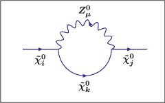
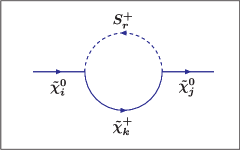
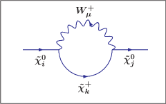
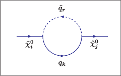
In the regime of renormalizable quantum field theories, stability of any tree level analysis must be re-examined in the light of radiative corrections. Following this prescription, the results of neutrino masses and mixing will be more robust, once tree level analysis is further improved by incorporating radiative corrections. The radiative corrections may have sizable effect on the neutrino data at one-loop level. Thus, although all three SM neutrinos acquire non-zero masses in the μν𝜇𝜈\mu\nuSSM even at the tree level [73], it is interesting to investigate the fate of those tree level masses and mixing when exposed to one-loop corrections. With this in view, in this section we perform a systematic study of the neutrino mass and mixing with all possible one-loop corrections both analytically and numerically. In the subsequent sections, while showing the results of one-loop corrections, we try to explain the deviations (which may or may not be prominent) from the tree level analysis. The complete set of one-loop diagrams are shown in figure1. Before going into the details, let us discuss certain relevant issues of one-loop correction and renormalization for the neutralino-neutrino sector. The most general one-loop contribution to the unrenormalized neutralino-neutrino two-point function can be expressed as

i𝚺χ~0χ~0ij(p)=i{[PLΣijL(p2)+PRΣijR(p2)][PLΠijL(p2)+PRΠijR(p2)]},𝑖subscriptsuperscript𝚺𝑖𝑗superscript~𝜒0superscript~𝜒0𝑝𝑖italic-p̸delimited-[]subscript𝑃𝐿subscriptsuperscriptΣ𝐿𝑖𝑗superscript𝑝2subscript𝑃𝑅subscriptsuperscriptΣ𝑅𝑖𝑗superscript𝑝2delimited-[]subscript𝑃𝐿subscriptsuperscriptΠ𝐿𝑖𝑗superscript𝑝2subscript𝑃𝑅subscriptsuperscriptΠ𝑅𝑖𝑗superscript𝑝2i{\bf\Sigma}^{ij}_{{\widetilde{\chi}}^{0}{\widetilde{\chi}}^{0}}(p)=i\{\displaystyle{\not}p\left[P_{L}{\Sigma^{L}_{ij}}(p^{2})+P_{R}{\Sigma^{R}_{ij}}(p^{2})\right]-\left[P_{L}{\Pi^{L}_{ij}}(p^{2})+P_{R}{\Pi^{R}_{ij}}(p^{2})\right]\}, (22)

where PLsubscript𝑃𝐿P_{L} and PRsubscript𝑃𝑅P_{R} are defined in eq.(109), i,j=1,,10formulae-sequence𝑖𝑗110i,~{}j~{}=~{}1,...,10 and p𝑝p is the external momentum. The unrenormalized self-energies ΣΣ\Sigma and ΠΠ\Pi depend on the squared external momentum (p2)superscript𝑝2(p^{2}). The generic self energies ΣijL(R),ΠijL(R)subscriptsuperscriptΣ𝐿𝑅𝑖𝑗subscriptsuperscriptΠ𝐿𝑅𝑖𝑗\Sigma^{L(R)}_{ij},~{}\Pi^{L(R)}_{ij} of the (Majorana) neutrino must be symmetric in its indices i,j𝑖𝑗i,j. The resulting one-loop corrected mass matrix using dimensional reduction (DR¯¯𝐷𝑅\overline{DR}) scheme [91] is given by

(χ~0tree+1loop)ij=mχ~0(μR)δij+12(Π~ijV(mi2)+Π~ijV(mj2)mχ~i0Σ~ijV(mi2)mχ~j0Σ~ijV(mj2)),superscriptsubscriptsuperscripttree1loopsuperscript~𝜒0𝑖𝑗subscript𝑚superscript~𝜒0subscript𝜇𝑅superscript𝛿𝑖𝑗12subscriptsuperscript~Π𝑉𝑖𝑗subscriptsuperscript𝑚2𝑖subscriptsuperscript~Π𝑉𝑖𝑗subscriptsuperscript𝑚2𝑗subscript𝑚subscriptsuperscript~𝜒0𝑖subscriptsuperscript~Σ𝑉𝑖𝑗subscriptsuperscript𝑚2𝑖subscript𝑚subscriptsuperscript~𝜒0𝑗subscriptsuperscript~Σ𝑉𝑖𝑗subscriptsuperscript𝑚2𝑗(\mathcal{M}^{\rm{tree+1-loop}}_{{\widetilde{\chi}}^{0}})^{ij}={m}_{{\widetilde{\chi}}^{0}}(\mu_{R})\delta^{ij}+{\frac{1}{2}}\left(\widetilde{\Pi}^{V}_{ij}({{m^{2}_{i}}})+\widetilde{\Pi}^{V}_{ij}({{m^{2}_{j}}})-{m_{{\widetilde{\chi}}^{0}_{i}}}{\widetilde{\Sigma}^{V}_{ij}}({{m^{2}_{i}}})-{m_{{\widetilde{\chi}}^{0}_{j}}}{\widetilde{\Sigma}^{V}_{ij}}({{m^{2}_{j}}})\right), (23)

with

Σ~ijVsubscriptsuperscript~Σ𝑉𝑖𝑗\displaystyle\widetilde{\Sigma}^{V}_{ij} =\displaystyle= 12(Σ~ijL+Σ~ijR),12subscriptsuperscript~Σ𝐿𝑖𝑗subscriptsuperscript~Σ𝑅𝑖𝑗\displaystyle\frac{1}{2}(\widetilde{\Sigma}^{L}_{ij}+\widetilde{\Sigma}^{R}_{ij}),
Π~ijVsubscriptsuperscript~Π𝑉𝑖𝑗\displaystyle\widetilde{\Pi}^{V}_{ij} =\displaystyle= 12(Π~ijL+Π~ijR).12subscriptsuperscript~Π𝐿𝑖𝑗subscriptsuperscript~Π𝑅𝑖𝑗\displaystyle\frac{1}{2}(\widetilde{\Pi}^{L}_{ij}+\widetilde{\Pi}^{R}_{ij}). (24)

where the tree level neutralino mass (mχ~0)subscript𝑚superscript~𝜒0({m}_{{\widetilde{\chi}}^{0}}) is defined at the renormalization scale μRsubscript𝜇𝑅\mu_{R}, set at the electroweak scale. Here, the word neutralino mass stands for all the ten eigenvalues of the 10×10101010\times 10 neutralino mass matrix. The self-energies Σ,ΠΣΠ\Sigma,~{}\Pi are also renormalized in the DR¯¯𝐷𝑅\overline{DR} scheme [91] and denoted by Σ~~Σ\widetilde{\Sigma} and Π~~Π\widetilde{\Pi} respectively. The detailed expressions of Σ~ijVsubscriptsuperscript~Σ𝑉𝑖𝑗\widetilde{\Sigma}^{V}_{ij} and Π~ijVsubscriptsuperscript~Π𝑉𝑖𝑗\widetilde{\Pi}^{V}_{ij} are given in appendix F.

3.4 Radiative corrections to neutrino mass terms

In this section we consider the effect of radiative corrections to the light neutrino masses. Let us recapitulate some of the earlier work regarding one-loop corrections to the neutralino-neutrino sector. The complete set of radiative corrections to the neutralino mass matrix in the RPsubscript𝑅𝑃R_{P} conserving MSSM was discussed in ref.[92], and the leading order neutrino masses has been derived in ref.[6]. One-loop radiative corrections to the neutrino-neutralino mass matrix in the context of a RPsubscript𝑅𝑃R_{P}-violating model were calculated in ref.[25] using ’t-Hooft-Feynman gauge. In ref.[42], Rξsubscript𝑅𝜉R_{\xi} gauge has been used to compute the corrections to the neutrino-neutralino mass matrix at one-loop level in an Rpsubscript𝑅𝑝R_{p}-violating scenario. Neutrino mass generation at the one-loop level in other variants of RPsubscript𝑅𝑃R_{P}-violating MSSM has also been addressed in refs. [39, 40, 50, 44, 45, 46, 47, 48, 19, 49, 51, 84, 99].

We begin by outlining the strategy of our analysis. We start with a general 10×10101010\times 10 neutralino matrix, with off-diagonal entries as well, which has a seesaw structure in the flavour-basis (see eq.(7)). Schematically, we can rewrite eq.(7) as,

n=(MfmDfTmDf0),subscript𝑛subscript𝑀𝑓subscriptsuperscript𝑚𝑇subscript𝐷𝑓subscript𝑚subscript𝐷𝑓0\mathcal{M}_{n}=\left(\begin{array}[]{cc}M_{f}&m^{T}_{D_{f}}\\ m_{D_{f}}&0\end{array}\right), (25)

where the orders of the block matrices are as those indicated in eq.(7), and the subscript ‘f𝑓f’ denotes the flavour basis. Here Mfsubscript𝑀𝑓M_{f} stands for the 7×7777\times 7 Majorana mass matrix of the heavy states, while mDfsubscript𝑚subscript𝐷𝑓m_{D_{f}} contains the 3×7373\times 7 Dirac type masses for the left handed neutrinos. In the next step, instead of utilising the seesaw structure of this matrix to generate the effective light neutrino mass matrix for the three active light neutrino species, we diagonalize the entire 10×10101010\times 10 matrix nsubscript𝑛\mathcal{M}_{n}. The diagonal 10×10101010\times 10 matrix MD0subscriptsuperscript𝑀0𝐷M^{0}_{D} thus contains tree level neutralino masses, which we symbolically write as

D0=(Mm00mm),superscriptsubscript𝐷0subscript𝑀𝑚00subscript𝑚𝑚\mathcal{M}_{D}^{0}=\left(\begin{array}[]{cc}M_{m}&0\\ 0&m_{m}\end{array}\right), (26)

where Mm(mm)subscript𝑀𝑚subscript𝑚𝑚M_{m}~{}(m_{m}) are the masses of the heavy states (left handed neutrinos). At this stage we turn on all possible one-loop interactions, so that the 10×10101010\times 10 matrix D0superscriptsubscript𝐷0\mathcal{M}_{D}^{0} picks up radiatively generated entries, both diagonal and off-diagonal. The resulting one-loop corrected Lagrangian for the neutralino mass terms, following eq.(6), can be written as

=12χ~0T(D0+1)χ~0+H.c.,superscript12superscript~𝜒superscript0𝑇subscriptsuperscript0𝐷superscript1superscript~𝜒0H.c.{\mathcal{L}^{\prime}}=-\frac{1}{2}{{\widetilde{\chi}^{0^{T}}}}\left(\mathcal{M}^{0}_{D}+\mathcal{M}^{1}\right){\widetilde{\chi}^{0}}+\text{H.c.}, (27)

where 1superscript1\mathcal{M}^{1} contains the effect of one-loop corrections. The 10×10101010\times 10 matrix D0subscriptsuperscript0𝐷\mathcal{M}^{0}_{D} is diagonal, but the matrix 1superscript1\mathcal{M}^{1} is a general symmetric matrix with off diagonal entries.

One can rewrite the above equation, using eqs.(10 and 11), as

=12Ψ0T(n+NT1N)Ψ0+H.c..superscript12superscriptsuperscriptΨ0𝑇subscript𝑛superscript𝑁𝑇superscript1𝑁superscriptΨ0H.c.{\mathcal{L}^{\prime}}=-\frac{1}{2}{{\Psi^{0}}^{T}}\left(\mathcal{M}_{n}+N^{T}\mathcal{M}^{1}N\right){\Psi^{0}}+\text{H.c.}. (28)

This is nothing but the one-loop corrected neutralino mass term in the Lagrangian in the flavour basis. Symbolically,

=12Ψ0TΨ0+H.c.,superscript12superscriptsuperscriptΨ0𝑇superscriptsuperscriptΨ0H.c.{\mathcal{L}^{\prime}}=-\frac{1}{2}{{\Psi^{0}}^{T}}\mathcal{M}^{\prime}{\Psi^{0}}+\text{H.c.}, (29)

with the 10×10101010\times 10 matrix superscript\mathcal{M}^{\prime} having the form

=(Mf+ΔMf(mDf+ΔmDf)TmDf+ΔmDfΔmf).superscriptsubscript𝑀𝑓Δsubscript𝑀𝑓superscriptsubscript𝑚subscript𝐷𝑓Δsubscript𝑚subscript𝐷𝑓𝑇subscript𝑚subscript𝐷𝑓Δsubscript𝑚subscript𝐷𝑓Δsubscript𝑚𝑓\mathcal{M}^{\prime}=\left(\begin{array}[]{cc}M_{f}+\Delta{M}_{f}&(m_{D_{f}}+\Delta{m_{D_{f}}})^{T}\\ m_{D_{f}}+\Delta{m_{D_{f}}}&\Delta{m}_{f}\end{array}\right). (30)

The quantities ΔMfΔsubscript𝑀𝑓\Delta{M}_{f} and ΔmfΔsubscript𝑚𝑓\Delta{m}_{f} stand for one-loop corrections to the heavy neutralino states and light neutrino states respectively, in the flavour basis Ψ0superscriptΨ0\Psi^{0}. The entity ΔmDfΔsubscript𝑚subscript𝐷𝑓\Delta{m_{D_{f}}} arises because of the off diagonal interactions, i.e. between the heavy neutralinos and the light neutrinos, in the same basis. Note that all of ΔMfΔsubscript𝑀𝑓\Delta M_{f}, ΔmDfΔsubscript𝑚subscript𝐷𝑓\Delta m_{D_{f}}, ΔmfΔsubscript𝑚𝑓\Delta m_{f} in the χ0subscript𝜒0\chi_{0} basis are given by the second term on the right hand side of eq.(23). We suitably transform them into the basis Ψ0superscriptΨ0\Psi^{0} with the help of neutralino mixing matrix N𝑁N. Interestingly, the matrix superscript\mathcal{M}^{\prime} once again possesses a seesaw structure, and one can therefore write down the one-loop corrected effective light neutrino mass matrix as

(Mν)effΔmf(mDf+ΔmDf)(Mf+ΔMf)1((mDf+ΔmDf)T).subscriptsuperscript𝑀superscript𝜈effΔsubscript𝑚𝑓subscript𝑚subscript𝐷𝑓Δsubscript𝑚subscript𝐷𝑓superscriptsubscript𝑀𝑓Δsubscript𝑀𝑓1superscriptsubscript𝑚subscript𝐷𝑓Δsubscript𝑚subscript𝐷𝑓𝑇({M}^{\nu^{\prime}})_{\rm{eff}}\approx\Delta{m}_{f}-(m_{D_{f}}+\Delta{m_{D_{f}}})(M_{f}+\Delta{M}_{f})^{-1}((m_{D_{f}}+\Delta{m_{D_{f}}})^{T}). (31)

Let us now present an approximate form of eq.(31). For simplicity, let us begin by assuming the quantities present in eq.(31) to be c-numbers (not matrices). In addition, assume MfΔMfmuch-greater-thansubscript𝑀𝑓Δsubscript𝑀𝑓M_{f}\gg\Delta{M}_{f} (justified later), so that eq.(31) may be written as,

(Mν)effΔmfδ×Mf{(mDfMf)2+2(mDfMf)(ΔmDfMf)+(ΔmDfMf)2},subscriptsuperscript𝑀superscript𝜈effΔsubscript𝑚𝑓𝛿subscript𝑀𝑓superscriptsubscript𝑚subscript𝐷𝑓subscript𝑀𝑓22subscript𝑚subscript𝐷𝑓subscript𝑀𝑓Δsubscript𝑚subscript𝐷𝑓subscript𝑀𝑓superscriptΔsubscript𝑚subscript𝐷𝑓subscript𝑀𝑓2({M}^{\nu^{\prime}})_{\rm{eff}}\approx\Delta{m}_{f}-\delta\times{M_{f}}\left\{\left(\frac{m_{D_{f}}}{M_{f}}\right)^{2}+2\left(\frac{m_{D_{f}}}{M_{f}}\right)\left(\frac{\Delta m_{D_{f}}}{M_{f}}\right)+\left(\frac{\Delta m_{D_{f}}}{M_{f}}\right)^{2}\right\}, (32)

with δ=(1ΔMfMf)𝛿1Δsubscript𝑀𝑓subscript𝑀𝑓\delta=\left(1-\frac{\Delta M_{f}}{M_{f}}\right). Now, even when ΔmDfΔsubscript𝑚subscript𝐷𝑓\Delta m_{D_{f}} similar-to\sim 116π2116superscript𝜋2\frac{1}{16\pi^{2}} mDfsubscript𝑚subscript𝐷𝑓m_{D_{f}} and ΔMfΔsubscript𝑀𝑓\Delta M_{f} similar-to\sim 116π2116superscript𝜋2\frac{1}{16\pi^{2}} Mfsubscript𝑀𝑓M_{f}, eq.(32) looks like

(Mν)effΔmfMf(1116π2){(mDfMf)2+216π2(mDfMf)2+1256π4(mDfMf)2}.subscriptsuperscript𝑀superscript𝜈effΔsubscript𝑚𝑓subscript𝑀𝑓1116superscript𝜋2superscriptsubscript𝑚subscript𝐷𝑓subscript𝑀𝑓2216superscript𝜋2superscriptsubscript𝑚subscript𝐷𝑓subscript𝑀𝑓21256superscript𝜋4superscriptsubscript𝑚subscript𝐷𝑓subscript𝑀𝑓2({M}^{\nu^{\prime}})_{\rm{eff}}\approx\Delta{m}_{f}-{M_{f}}\left(1-\frac{1}{16\pi^{2}}\right)\left\{\left(\frac{m_{D_{f}}}{M_{f}}\right)^{2}+\frac{2}{16\pi^{2}}\left(\frac{m_{D_{f}}}{M_{f}}\right)^{2}+\frac{1}{256\pi^{4}}\left(\frac{m_{D_{f}}}{M_{f}}\right)^{2}\right\}. (33)

Thus, up to a very good approximation one can rewrite eq.(33) as

(Mν)effΔmfMf(mDfMf)2.subscriptsuperscript𝑀superscript𝜈effΔsubscript𝑚𝑓subscript𝑀𝑓superscriptsubscript𝑚subscript𝐷𝑓subscript𝑀𝑓2({M}^{\nu^{\prime}})_{\rm{eff}}\approx\Delta{m}_{f}-{M_{f}}\left(\frac{m_{D_{f}}}{M_{f}}\right)^{2}. (34)

Reimposing the matrix structure and using eq.(17), eq.(34) can be modified as,

(Mν)effΔmf+Mνseesaw.subscriptsuperscript𝑀superscript𝜈effΔsubscript𝑚𝑓subscriptsuperscript𝑀𝑠𝑒𝑒𝑠𝑎𝑤𝜈({M}^{\nu^{\prime}})_{\rm{eff}}\approx\Delta{m}_{f}+{M^{seesaw}_{\nu}}. (35)

The eigenvalues of the 3×3333\times 3 one-loop corrected neutrino mass matrix (Mν)effsubscriptsuperscript𝑀superscript𝜈eff({M}^{\nu^{\prime}})_{\rm{eff}} thus correspond to one-loop corrected light neutrino masses. In conclusion, it is legitimate to calculate one-loop corrections to the 3×3333\times 3 light neutrino mass matrix only, and diagonalize it to get the corresponding one-loop corrected mass eigenvalues.

Let us denote the one-loop corrections to the masses of heavy neutralinos and light neutrinos in the basis χ~0superscript~𝜒0\widetilde{\chi}^{0} by ΔMΔ𝑀\Delta M and ΔmΔ𝑚\Delta m respectively. The one-loop corrections arising from neutralino-neutrino interactions is denoted by ΔmDΔsubscript𝑚𝐷\Delta m_{D} in the same basis. The tree level neutralino mixing matrix N𝑁N can then be written as,

N=(N~7×7N~7×3N~3×7N~3×3),𝑁subscript~𝑁77subscript~𝑁73subscript~𝑁37subscript~𝑁33N=\left(\begin{array}[]{cc}\widetilde{N}_{7\times 7}&\widetilde{N}_{7\times 3}\\ \widetilde{N}_{3\times 7}&\widetilde{N}_{3\times 3}\end{array}\right), (36)

where the entries of the matrices N~7×3,N~3×7subscript~𝑁73subscript~𝑁37\widetilde{N}_{7\times 3},~{}\widetilde{N}_{3\times 7} are 𝒪similar-toabsent𝒪\sim\cal{O} (mDν/Mχ~0)superscriptsubscript𝑚𝐷𝜈subscript𝑀superscript~𝜒0({m_{D}^{\nu}}/{M_{\widetilde{\chi}^{0}}}), due to very small neutrino-neutralino mixing [93]. The quantities mDνsuperscriptsubscript𝑚𝐷𝜈m_{D}^{\nu} and Mχ~0subscript𝑀superscript~𝜒0M_{\widetilde{\chi}^{0}} represent the Dirac mass of neutrino and the Majorana mass of neutralino. From eq.(28), it is easy to figure out the relation between ΔmΔ𝑚\Delta m and ΔmfΔsubscript𝑚𝑓\Delta m_{f} as,

Δmf=N~7×3TΔMN~7×3+N~7×3TΔmDTN~3×3+N~3×3TΔmDN~7×3+N~3×3TΔmN~3×3.Δsubscript𝑚𝑓superscriptsubscript~𝑁73𝑇Δ𝑀subscript~𝑁73superscriptsubscript~𝑁73𝑇Δsuperscriptsubscript𝑚𝐷𝑇subscript~𝑁33superscriptsubscript~𝑁33𝑇Δsubscript𝑚𝐷subscript~𝑁73superscriptsubscript~𝑁33𝑇Δ𝑚subscript~𝑁33\Delta m_{f}={\widetilde{N}_{7\times 3}^{T}}{\Delta M}{\widetilde{N}_{7\times 3}}+{\widetilde{N}_{7\times 3}^{T}}{\Delta m_{D}^{T}}{\widetilde{N}_{3\times 3}}+{\widetilde{N}_{3\times 3}^{T}}{\Delta m_{D}}{\widetilde{N}_{7\times 3}}+{\widetilde{N}_{3\times 3}^{T}}{\Delta m}{\widetilde{N}_{3\times 3}}. (37)

Typically, for a Dirac neutrino, the mass is <fragmentsfragmentssimilar-to\mathrel{\mathchoice{\vbox{\offinterlineskip\halign{$\m@th\displaystyle\hfil#\hfil$\cr<\crcr\sim\crcr} }}{\vbox{\offinterlineskip\halign{$\m@th\textstyle\hfil#\hfil$\cr<\crcr\sim\crcr} }}{\vbox{\offinterlineskip\halign{$\m@th\scriptstyle\hfil#\hfil$\cr<\crcr\sim\crcr} }}{\vbox{\offinterlineskip\halign{$\m@th\scriptscriptstyle\hfil#\hfil$\cr<\crcr\sim\crcr} }}} 𝒪𝒪\cal{O} (104GeV)superscript104GeV(10^{-4}~{}\rm{GeV}), while for a neutralino, the mass is similar-to\sim 𝒪𝒪\cal{O} (102GeV)superscript102GeV(10^{2}~{}\rm{GeV}). This means that the entries of the off-diagonal blocks in eq.(36) are <fragmentsfragmentssimilar-to\mathrel{\mathchoice{\vbox{\offinterlineskip\halign{$\m@th\displaystyle\hfil#\hfil$\cr<\crcr\sim\crcr} }}{\vbox{\offinterlineskip\halign{$\m@th\textstyle\hfil#\hfil$\cr<\crcr\sim\crcr} }}{\vbox{\offinterlineskip\halign{$\m@th\scriptstyle\hfil#\hfil$\cr<\crcr\sim\crcr} }}{\vbox{\offinterlineskip\halign{$\m@th\scriptscriptstyle\hfil#\hfil$\cr<\crcr\sim\crcr} }}} 𝒪𝒪\cal{O} (106)superscript106(10^{-6}). Therefore, for all practical purposes, one can neglect the first three terms in comparison to the fourth term on the right hand side of eq.(37). Thus,

ΔmfN~3×3TΔmN~3×3.Δsubscript𝑚𝑓superscriptsubscript~𝑁33𝑇Δ𝑚subscript~𝑁33\Delta m_{f}\approx{\widetilde{N}_{3\times 3}^{T}}{\Delta m}{\widetilde{N}_{3\times 3}}. (38)

up to a very good approximation. With this in view, our strategy is to compute the one-loop corrections in the χ~0superscript~𝜒0\widetilde{\chi}^{0} basis first, and then use eq.(38) to obtain the corresponding corrections in the flavour basis. Finally, we diagonalize eq.(35) to obtain the one-loop corrected neutrino masses. We have performed all calculations in the ’t-Hooft-Feynman gauge. Let us also note in passing that the form of eq.(23) predicts off-diagonal entries (ij𝑖𝑗i\neq j). The off-diagonal elements are responsible for the mixing between diagonal entries, they become dominant only when (mχ~i0mχ~j0)(α4π)×someelectroweakscalemassless-than-or-similar-tosubscript𝑚subscriptsuperscript~𝜒0𝑖subscript𝑚subscriptsuperscript~𝜒0𝑗𝛼4𝜋someelectroweakscalemass\left({m}_{{\widetilde{\chi}}^{0}_{i}}-{m}_{{\widetilde{\chi}}^{0}_{j}}\right)~{}\lesssim(\frac{\alpha}{4\pi})\times{\rm{some~{}electroweak~{}scale~{}mass}}, and then, one can choose p2=m2¯=(m2χ~i0+m2χ~j0)/2superscript𝑝2¯superscript𝑚2subscriptsuperscript𝑚2subscriptsuperscript~𝜒0𝑖subscriptsuperscript𝑚2subscriptsuperscript~𝜒0𝑗2p^{2}=\overline{m^{2}}=({{m^{2}}_{{\widetilde{\chi}}^{0}_{i}}+{m^{2}}_{{\widetilde{\chi}}^{0}_{j}}})/2 for external momentum[25]. Thus, one can conclude that unless the tree level masses are degenerate, the off-diagonal radiative corrections can be neglected for all practical purposes, when at least one index i𝑖i or j𝑗j refers to a heavy states.

The self-energy corrections contain entries of the neutralino mixing matrix N𝑁N through the couplings Offbsuperscript𝑂𝑓superscript𝑓𝑏O^{ff^{\prime}b} (see, appendix E). This is because, the self energies Σ~𝑖𝑗subscript~𝛴𝑖𝑗{\it{\widetilde{\Sigma}}_{ij}} and Π~𝑖𝑗subscript~𝛱𝑖𝑗{\it{\widetilde{\Pi}}_{ij}} in general contain products of couplings of the form Oi..ffbOj..ffbO^{ff^{\prime}b}_{i..}O^{ff^{\prime}b}_{j..}. The matrix N𝑁N, on the other hand, contains the expansion parameter ξ𝜉\xi in the leading order (see eq.(15)). This observation, together with the help of eq.(65), help us to express the effective structure of the one-loop corrected neutrino mass matrix as,

[(ν)eff]ij=A1aiaj+A2cicj+A3(aicj+ajci),subscriptdelimited-[]subscriptsuperscriptsuperscript𝜈𝑒𝑓𝑓𝑖𝑗subscript𝐴1subscript𝑎𝑖subscript𝑎𝑗subscript𝐴2subscript𝑐𝑖subscript𝑐𝑗subscript𝐴3subscript𝑎𝑖subscript𝑐𝑗subscript𝑎𝑗subscript𝑐𝑖[(\mathcal{M}^{\nu^{\prime}})_{eff}]_{ij}=A_{1}a_{i}a_{j}+A_{2}c_{i}c_{j}+A_{3}(a_{i}c_{j}+a_{j}c_{i}), (39)

where aisubscript𝑎𝑖a_{i} and cisubscript𝑐𝑖c_{i} are given by eq.(14) and Aisubscript𝐴𝑖A_{i}’s are functions of our model parameters and the Passarino-Veltman functions (B0,B1)subscript𝐵0subscript𝐵1(B_{0},B_{1}) [94, 95, 96] defined in appendix G. The form of the loop corrected mass matrix thus obtained is identical to the tree level one (see, eq.(19)) with different coefficients A1subscript𝐴1A_{1}, A2subscript𝐴2A_{2} and A3subscript𝐴3A_{3} arising now.

Note that the one-loop diagrams in figure1, contributing to the neutrino mass matrix are very similar to those obtained in bilinear R-parity violating scenario [42, 43, 44, 45, 50, 51]. However, it has been pointed out in Ref.[79], that there is a new significant contribution coming from the loops containing the neutral scalar and pseudoscalar with dominant singlet component. This contribution is proportional to the mass-splitting between the singlet scalar and pseudoscalar states [97, 98, 99]. The corresponding mass splittings for the doublet sneutrinos are much smaller [79].
Refer to caption
Refer to caption
Refer to caption
Refer to caption
Refer to caption
Refer to caption
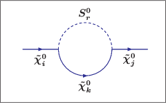
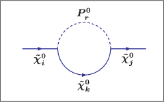
Figure 1: One-loop diagrams contributing to the neutralino masses. The various contributions are arising from (clockwise from top left) (a) neutralino-neutralino-neutral scalar loop, (b) neutralino-neutralino-neutral pseudoscalar loop, (c) neutralino-neutralino-Zμ0subscriptsuperscript𝑍0𝜇Z^{0}_{\mu} loop, (d) neutralino-chargino-charged scalar loop, (e) neutralino-chargino-Wμ±subscriptsuperscript𝑊plus-or-minus𝜇W^{\pm}_{\mu} loop, (f) neutralino-quark-squark loop.

3.5 Neutrino mixing

The unitary matrix which diagonalizes the 3×3333\times 3 light neutrino mass matrix, can be parametrized as [100],

𝒰νsubscript𝒰𝜈\displaystyle{\mathcal{U}_{\nu}} =\displaystyle= (c12c13s12c13s13s12c23c12s23s13c12c23s12s23s13s23c13s12s23c12c23s13c12s23s12c23s13c23c13),subscript𝑐12subscript𝑐13subscript𝑠12subscript𝑐13subscript𝑠13missing-subexpressionmissing-subexpressionmissing-subexpressionsubscript𝑠12subscript𝑐23subscript𝑐12subscript𝑠23subscript𝑠13subscript𝑐12subscript𝑐23subscript𝑠12subscript𝑠23subscript𝑠13subscript𝑠23subscript𝑐13missing-subexpressionmissing-subexpressionmissing-subexpressionsubscript𝑠12subscript𝑠23subscript𝑐12subscript𝑐23subscript𝑠13subscript𝑐12subscript𝑠23subscript𝑠12subscript𝑐23subscript𝑠13subscript𝑐23subscript𝑐13\displaystyle\left(\begin{array}[]{ccc}{c_{12}}{c_{13}}&{s_{12}}{c_{13}}&{s_{13}}\\ \\ -{s_{12}}{c_{23}}-{c_{12}}{s_{23}}{s_{13}}&{c_{12}}{c_{23}}-{s_{12}}{s_{23}}{s_{13}}&{s_{23}}{c_{13}}\\ \\ {s_{12}}{s_{23}}-{c_{12}}{c_{23}}{s_{13}}&-{c_{12}}{s_{23}}-{s_{12}}{c_{23}}{s_{13}}&{c_{23}}{c_{13}}\end{array}\right), (45)

provided the charged lepton sector is in the mass-basis (see appendix D). Here cij=cosθijsubscript𝑐𝑖𝑗subscript𝜃𝑖𝑗c_{ij}=\cos{\theta_{ij}}, sij=sinθijsubscript𝑠𝑖𝑗subscript𝜃𝑖𝑗s_{ij}=\sin{\theta_{ij}}, and all CP𝐶𝑃CP violating phases (Dirac or Majorana) are set to zero. The experimental data on neutrino oscillations [101, 102] indicate that a bilarge pattern of mixing of neutrinos may be preferred, which means that two of the mixing angles must be large. As a first approximation, one can work with θ23=45subscript𝜃23superscript45\theta_{23}=45^{\circ}, sinθ12=13subscript𝜃1213\sin{\theta_{12}}={\frac{1}{\sqrt{3}}} and θ130subscript𝜃13superscript0\theta_{13}\approx 0^{\circ}, which is often referred to as the ‘tribimaximal structure’ [103]. Following the above discussions, we can write down the tree level PMNS matrix 𝒰νsubscript𝒰𝜈{\mathcal{U}_{\nu}} as,

𝒰ν=N~T3×3,{\mathcal{U}_{\nu}}={\widetilde{N}^{{\prime}^{T}}}_{3\times 3}, (46)

where N~3×3subscriptsuperscript~𝑁33{\widetilde{N}^{{\prime}}}_{3\times 3} is the matrix that diagonalizes the tree level mass matrix Mνseesawsubscriptsuperscript𝑀𝑠𝑒𝑒𝑠𝑎𝑤𝜈M^{seesaw}_{\nu} (eq.(17)).

Similarly, the 3×3333\times 3 unitary matrix that diagonalizes the one-loop corrected neutrino mass matrix (Mν)effsubscriptsuperscript𝑀superscript𝜈eff({M}^{\nu^{\prime}})_{\rm{eff}} (eq.(35)), can be denoted as 𝒰νsubscriptsuperscript𝒰𝜈\mathcal{U}^{\prime}_{\nu}. Symbolically

𝒰ν1(Mν)eff𝒰ν=diag(m1,m2,m3),{\mathcal{U}^{{\prime}^{-1}}_{\nu}}({M}^{\nu^{\prime}})_{\rm{eff}}{\mathcal{U}^{\prime}_{\nu}}={\rm{diag}}(m^{\prime}_{1},~{}m^{\prime}_{2},~{}m^{\prime}_{3}), (47)

with m1subscriptsuperscript𝑚1m^{\prime}_{1}, m2subscriptsuperscript𝑚2m^{\prime}_{2}, m3subscriptsuperscript𝑚3m^{\prime}_{3} as the three one-loop corrected light neutrino masses. A similar relation for the tree level calculation is given by the second equation of (3.1), with misubscript𝑚𝑖m_{i}’s as the tree level neutrino masses.

When we include one-loop corrections, the PMNS matrix 𝒰νsubscriptsuperscript𝒰𝜈{\mathcal{U}^{\prime}_{\nu}} is defined as

𝒰ν=N~T3×3,{\mathcal{U}^{\prime}_{\nu}}={\widetilde{N}^{{\prime\prime}^{T}}}_{3\times 3}, (48)

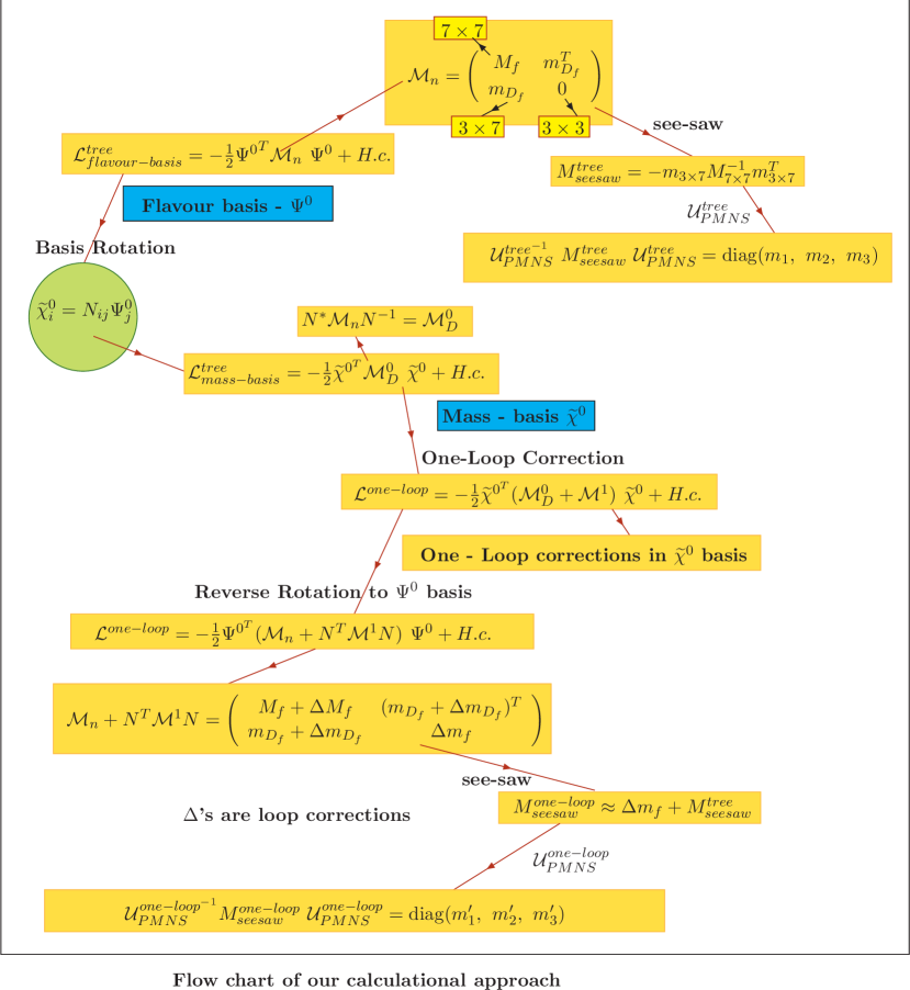
where N~′′3×3subscriptsuperscript~𝑁′′33{\widetilde{N}^{{\prime\prime}}}_{3\times 3} is the matrix which diagonalizes the one-loop corrected mass matrix (Mν)effsubscriptsuperscript𝑀superscript𝜈eff({M}^{\nu^{\prime}})_{\rm{eff}}. The scheme for obtaining the loop-corrected neutrino mixing matrix is shown in figure2.
Refer to caption
Figure 2: Flow chart of the calculational procedure that we have followed in order to calculate the neutrino masses and mixing at the tree level and at one-loop. Here 𝒰PMNSoneloopsubscriptsuperscript𝒰𝑜𝑛𝑒𝑙𝑜𝑜𝑝𝑃𝑀𝑁𝑆{\mathcal{U}^{one-loop}_{PMNS}} = 𝒰νsubscriptsuperscript𝒰𝜈{\mathcal{U}^{\prime}_{\nu}}, 𝒰PMNStreesubscriptsuperscript𝒰𝑡𝑟𝑒𝑒𝑃𝑀𝑁𝑆{\mathcal{U}^{tree}_{PMNS}} = 𝒰νsubscript𝒰𝜈{\mathcal{U}_{\nu}}, flavourbasistree=neutralmasssubscriptsuperscript𝑡𝑟𝑒𝑒𝑓𝑙𝑎𝑣𝑜𝑢𝑟𝑏𝑎𝑠𝑖𝑠subscriptsuperscript𝑚𝑎𝑠𝑠𝑛𝑒𝑢𝑡𝑟𝑎𝑙\mathcal{L}^{tree}_{flavour-basis}=\mathcal{L}^{mass}_{neutral}, Mseesawtree=Mνseesawsubscriptsuperscript𝑀𝑡𝑟𝑒𝑒𝑠𝑒𝑒𝑠𝑎𝑤subscriptsuperscript𝑀𝑠𝑒𝑒𝑠𝑎𝑤𝜈M^{tree}_{seesaw}=M^{seesaw}_{\nu}, oneloop=superscript𝑜𝑛𝑒𝑙𝑜𝑜𝑝superscript\mathcal{L}^{one-loop}=\mathcal{L}^{\prime} and Mseesawoneloop=(Mν)effsubscriptsuperscript𝑀𝑜𝑛𝑒𝑙𝑜𝑜𝑝𝑠𝑒𝑒𝑠𝑎𝑤subscriptsuperscript𝑀superscript𝜈𝑒𝑓𝑓M^{one-loop}_{seesaw}=(M^{\nu^{\prime}})_{eff} in the text.

4 Numerical results of neutrino mass and mixing

In this section we present and explain the results of our numerical analysis. Let us begin with a brief outline of the different well known schemes of light neutrino masses as favoured by experiments. These are (i) The normal hierarchy: m1<m2Δmsolar2subscript𝑚1subscript𝑚2similar-toΔsubscriptsuperscript𝑚2𝑠𝑜𝑙𝑎𝑟m_{1}<m_{2}\sim\sqrt{\Delta m^{2}_{solar}}m3|Δmatm2|similar-tosubscript𝑚3Δsubscriptsuperscript𝑚2𝑎𝑡𝑚m_{3}\sim\sqrt{|\Delta m^{2}_{atm}|}, (ii) The inverted hierarchy: m1m2|Δmatm2|subscript𝑚1subscript𝑚2similar-toΔsubscriptsuperscript𝑚2𝑎𝑡𝑚m_{1}\approx m_{2}\sim\sqrt{|\Delta m^{2}_{atm}|}, m3|Δmatm2|much-less-thansubscript𝑚3Δsubscriptsuperscript𝑚2𝑎𝑡𝑚m_{3}\ll\sqrt{|\Delta m^{2}_{atm}|} and (iii) The quasi-degenerate pattern: m1m2m3|Δmatm2|subscript𝑚1subscript𝑚2subscript𝑚3much-greater-thanΔsubscriptsuperscript𝑚2𝑎𝑡𝑚m_{1}\approx m_{2}\approx m_{3}\gg\sqrt{|\Delta m^{2}_{atm}|}, where m1subscript𝑚1m_{1}, m2subscript𝑚2m_{2} and m3subscript𝑚3m_{3} are the three light neutrino masses. Here, Δmsolar2m22m12Δsubscriptsuperscript𝑚2𝑠𝑜𝑙𝑎𝑟subscriptsuperscript𝑚22subscriptsuperscript𝑚21\Delta m^{2}_{solar}\equiv m^{2}_{2}-m^{2}_{1} and  Δmatm2m32m22(m12)Δsubscriptsuperscript𝑚2𝑎𝑡𝑚subscriptsuperscript𝑚23subscriptsuperscript𝑚22subscriptsuperscript𝑚21\Delta m^{2}_{atm}\equiv m^{2}_{3}-m^{2}_{2}(m^{2}_{1}) for Normal (inverted) Hierarchy. The possibility of more than one scheme of neutrino masses essentially stems from our lack of knowledge of the signs of the squared mass differences, or the value of individual masses. Such being the case, the numerical analysis must be subjected to address all the three probable schemes.

The numerical calculations have been performed with the help of a code developed by us in Fortran and the results have been cross-checked using another Mathematica [104] based program we developed. In the code, we keep the left handed sneutrino VEVs (vsuperscript𝑣v^{\prime}), the right handed sneutrino VEVs (vc)superscript𝑣𝑐(v^{c}) and the neutrino Yukawa couplings (Yν)subscript𝑌𝜈(Y_{\nu}) as free input variables, and then scan over the parameter space for a region consistent with the three flavour global neutrino data. For all our numerical analysis we keep the right handed sneutrino VEVs fixed at some chosen values (see table 1). The only exception to this is when we study the correlation of neutrino data with the bilinear RPsubscript𝑅𝑃R_{P}-violating parameter εi=Yνijvjcsubscript𝜀𝑖subscriptsuperscript𝑌𝑖𝑗𝜈subscriptsuperscript𝑣𝑐𝑗\varepsilon_{i}=Y^{ij}_{\nu}v^{c}_{j}. For that particular study, we vary the right handed sneutrino VEVs (consistent with EWSB conditions) within the mass scale –895GeV895GeV895~{}\rm{GeV} to –565GeV565GeV565~{}\rm{GeV}. The table 1 shows our choice of the sample parameters for the numerical analysis. The relation between the gaugino soft masses M1subscript𝑀1M_{1} and M2subscript𝑀2M_{2} are assumed to be GUT (grand unified theory) motivated, so that, at the electroweak scale, we have M1:M2=1:2:subscript𝑀1subscript𝑀21:2M_{1}:M_{2}~{}=~{}1:2. We choose M1=110GeVsubscript𝑀1110GeVM_{1}~{}=~{}110~{}\rm{GeV}.

tanβ𝛽\beta λ𝜆\lambda Aλλsubscript𝐴𝜆𝜆A_{\lambda}\lambda κ𝜅\kappa Aκκsubscript𝐴𝜅𝜅A_{\kappa}\kappa (AνYν)iisuperscriptsubscript𝐴𝜈subscript𝑌𝜈𝑖𝑖(A_{\nu}Y_{\nu})^{ii} (me~c2)superscriptsubscript𝑚superscript~𝑒𝑐2(m_{\tilde{e}^{c}}^{2}) vicsubscriptsuperscript𝑣𝑐𝑖v^{c}_{i}
10 0.10 1TeV×λ1TeV𝜆-1\rm{TeV}\times\lambda 0.45 1TeV×κ1TeV𝜅1\rm{TeV}\times\kappa 1TeV×Yνii1TeVsubscriptsuperscriptYii𝜈1\rm{TeV}\times Y^{ii}_{\nu} 3002GeV2superscript3002superscriptGeV2300^{2}~{}\rm{GeV}^{2} 595GeV595GeV-595~{}\rm{GeV}
Table 1: Choice of parameters for numerical analysis consistent with the EWSB conditions.

We scanned the parameter space comprising of the left handed sneutrino VEVs and the neutrino Yukawa couplings extensively and found certain ranges of these parameters appropriate for various hierarchical schemes of the light neutrino masses. In table 2, some sample values for these six parameters for the different mass schemes of neutrinos are given. These values are just for illustration and the parameters were scanned around these numbers to generate the plots shown in this section. The other relevant parameters have values as mentioned in table 1.

Yνii×107subscriptsuperscript𝑌𝑖𝑖𝜈superscript107Y^{ii}_{\nu}\times 10^{7} vi×105(GeV)subscriptsuperscript𝑣𝑖superscript105GeVv^{\prime}_{i}\times 10^{5}(\rm{GeV})
Yν11subscriptsuperscript𝑌11𝜈Y^{11}_{\nu} Yν22subscriptsuperscript𝑌22𝜈Y^{22}_{\nu} Yν33subscriptsuperscript𝑌33𝜈Y^{33}_{\nu} v1subscriptsuperscript𝑣1v^{\prime}_{1} v2subscriptsuperscript𝑣2v^{\prime}_{2} v3subscriptsuperscript𝑣3v^{\prime}_{3}
Normal hierarchy 3.550 5.400 1.650 0.730 10.100 12.450
Inverted hierarchy 12.800 3.300 4.450 8.350 8.680 6.400
Table 2: Values of neutrino Yukawa couplings and left handed sneutrino VEVs, used as sample parameter points for numerical calculations. These are the values around which the corresponding parameters were varied.

While fitting the three flavour global neutrino data, we consider constraints arising from the oscillation data as well as from the non-oscillation data. We probe the effects of these constraints for both tree level and (tree + one-loop) level analyses. The oscillation data constrain the solar and atmospheric mass squared differences, namely, Δmsolar2Δsubscriptsuperscript𝑚2𝑠𝑜𝑙𝑎𝑟\Delta m^{2}_{solar} and Δmatm2Δsubscriptsuperscript𝑚2𝑎𝑡𝑚\Delta m^{2}_{atm}, and three neutrino mixing angles θ13,θ12,θ23subscript𝜃13subscript𝜃12subscript𝜃23\theta_{13},~{}\theta_{12},~{}\theta_{23}. The present 3σ𝜎\sigma limits are [2, 3],

7.05×10⁵eV2Δmsolar27.05superscript105superscripteV2Δsubscriptsuperscript𝑚2𝑠𝑜𝑙𝑎𝑟\displaystyle 7.05\times 10^{-5}{\rm eV}^{2}\leq\Delta m^{2}_{solar} 8.34×10⁵eV2,absent8.34superscript105superscripteV2\displaystyle\leq 8.34\times 10^{-5}{\rm eV}^{2},
2.07×10³eV2|Δmatm2|2.07superscript103superscripteV2Δsubscriptsuperscript𝑚2𝑎𝑡𝑚\displaystyle 2.07\times 10^{-3}{\rm eV}^{2}\leq|\Delta m^{2}_{atm}| 2.75×10³eV2,absent2.75superscript103superscripteV2\displaystyle\leq 2.75\times 10^{-3}{\rm eV}^{2},
0.25sin2θ120.25superscript2subscript𝜃12\displaystyle 0.25\leq\sin^{2}\theta_{12} 0.37,absent0.37\displaystyle\leq 0.37,
0.36sin2θ230.36superscript2subscript𝜃23\displaystyle 0.36\leq\sin^{2}\theta_{23} 0.67,absent0.67\displaystyle\leq 0.67,
sin2θ13superscript2subscript𝜃13\displaystyle\sin^{2}\theta_{13} 0.056.absent0.056\displaystyle\leq 0.056.

The non-oscillation constraints follow from experiments like β𝛽\beta decay [105, 106, 107], neutrinoless double beta decay (0νββ)0𝜈𝛽𝛽(0\nu\beta\beta) [108, 109, 110] (this is also sensitive to Majorana nature and phases), and from cosmology [111]. Here we set all the Majorana phases to be zero, as we are dealing with a CPlimit-from𝐶𝑃CP-preserving situation.

The set of non-oscillation constraints are given as,

mβ=|𝒰νei|2mi2subscript𝑚𝛽superscriptsubscript𝒰subscript𝜈𝑒𝑖2subscriptsuperscript𝑚2𝑖\displaystyle m_{\beta}=\sqrt{\sum|{{\mathcal{U}_{\nu_{ei}}}}|^{2}m^{2}_{i}} <1.80eV(βdecay),absent1.80eV𝛽decay\displaystyle<1.80~{}\rm{eV}~{}~{}~{}~{}(\beta~{}decay),
0.00eVmββ=|𝒰νei2mi|0.00eVsubscript𝑚𝛽𝛽superscriptsubscript𝒰subscript𝜈𝑒𝑖2subscript𝑚𝑖\displaystyle 0.00~{}{\rm{eV}}\leq m_{\beta\beta}=|\sum{{\mathcal{U}_{\nu_{ei}}}}^{2}m_{i}| 0.25eV(0νββ),absent0.25eV0𝜈𝛽𝛽\displaystyle\leq 0.25~{}\rm{eV}~{}~{}~{}~{}(0\nu\beta\beta),
misubscript𝑚𝑖\displaystyle\sum m_{i} <1.30eV(cosmology),absent1.30eVcosmology\displaystyle<1.30~{}\rm{eV}~{}~{}~{}~{}(cosmology),

where misubscript𝑚𝑖m_{i}s are three light neutrino masses, and 𝒰νeisubscript𝒰subscript𝜈𝑒𝑖{\mathcal{U}_{\nu_{ei}}}s are the elements of the first row of the neutrino mixing matrix (see eq.(45)).

4.1 Normal hierarchy

In the normal hierarchical pattern of the three light neutrino masses, the atmospheric and the solar mass squared differences, given by Δmatm2=m32m22Δsubscriptsuperscript𝑚2𝑎𝑡𝑚subscriptsuperscript𝑚23subscriptsuperscript𝑚22\Delta m^{2}_{atm}=m^{2}_{3}-m^{2}_{2} and Δmsolar2=m22m12Δsubscriptsuperscript𝑚2𝑠𝑜𝑙𝑎𝑟subscriptsuperscript𝑚22subscriptsuperscript𝑚21\Delta m^{2}_{solar}=m^{2}_{2}-m^{2}_{1}, are largely governed by the higher mass squared in each case, namely, m32superscriptsubscript𝑚32m_{3}^{2} and m22superscriptsubscript𝑚22m_{2}^{2}, respectively. Before going into the discussion of the variation of the mass-squared values with the model parameter, some general remarks are in order. First of all, note that in eq.(14), if we choose visubscriptsuperscript𝑣𝑖v^{\prime}_{i} such that viYνiiv13λmuch-greater-thansubscriptsuperscript𝑣𝑖subscriptsuperscript𝑌𝑖𝑖𝜈subscript𝑣13𝜆v^{\prime}_{i}\gg\frac{Y^{ii}_{\nu}v_{1}}{3\lambda}, then bicisubscript𝑏𝑖subscript𝑐𝑖b_{i}\approx c_{i}[80]. Thus, for large visubscriptsuperscript𝑣𝑖v^{\prime}_{i}, we remind ourselves that in eq.(18), the effective light neutrino mass matrix has two types of seesaw structures [73]. The first one is the ordinary seesaw, given by

mνai2mνc,similar-tosubscript𝑚𝜈subscriptsuperscript𝑎2𝑖subscript𝑚superscript𝜈𝑐\displaystyle m_{\nu}\sim\frac{a^{2}_{i}}{m_{\nu^{c}}}, (51)

where ai=Yνiiv2subscript𝑎𝑖superscriptsubscript𝑌𝜈𝑖𝑖subscript𝑣2a_{i}=Y_{\nu}^{ii}v_{2} represents the Dirac mass term for neutrinos, and mνc=2κvcsubscript𝑚superscript𝜈𝑐2𝜅superscript𝑣𝑐m_{\nu^{c}}={2\kappa v^{c}} stands for the Majorana mass term of the right handed neutrino. The second type is called the gaugino seesaw, in which the role of the Dirac mass terms are played by g1cisubscript𝑔1subscript𝑐𝑖g_{1}c_{i} and g2cisubscript𝑔2subscript𝑐𝑖g_{2}c_{i}, where g1,g2subscript𝑔1subscript𝑔2g_{1},~{}g_{2} are the U(1)𝑈1U(1) and the SU(2)𝑆𝑈2SU(2) gauge couplings respectively and cisubscript𝑐𝑖c_{i} stands for the left handed sneutrino VEV visubscriptsuperscript𝑣𝑖v^{\prime}_{i}. The role of the Majorana masses are played by the gaugino soft masses M1,M2subscript𝑀1subscript𝑀2M_{1},~{}M_{2}. This seesaw relation is given as

mνsubscript𝑚𝜈\displaystyle m_{\nu} similar-to\displaystyle\sim (g1ci)2M1+(g2ci)2M2,superscriptsubscript𝑔1subscript𝑐𝑖2subscript𝑀1superscriptsubscript𝑔2subscript𝑐𝑖2subscript𝑀2\displaystyle\frac{(g_{1}c_{i})^{2}}{M_{1}}+\frac{(g_{2}c_{i})^{2}}{M_{2}}, (52)
similar-to\displaystyle\sim ci2M,subscriptsuperscript𝑐2𝑖𝑀\displaystyle\frac{c^{2}_{i}}{M},

where the subscript ‘i𝑖i=1,2,3e,μ,τformulae-sequenceabsent123𝑒𝜇𝜏=1,2,3\equiv e,\mu,\tau and M𝑀M is the reduced gaugino mass defined by

1M=g12M1+g22M2.1𝑀subscriptsuperscript𝑔21subscript𝑀1subscriptsuperscript𝑔22subscript𝑀2\displaystyle\frac{1}{M}=\frac{g^{2}_{1}}{M_{1}}+\frac{g^{2}_{2}}{M_{2}}. (53)

M𝑀M here plays the role of the effective heavy mass provided by the neutral electroweak gaugino sector, and the effect is closely analogous to Type-III seesaw mechanism[112]111We thank Anjan Joshipura for pointing this out to one of the authors in a private discussion.. As discussed after eq.(39), when one-loop corrections are added, the neutrino masses are still determined by the quantities ai2subscriptsuperscript𝑎2𝑖a^{2}_{i} and ci2subscriptsuperscript𝑐2𝑖c^{2}_{i} (bi2absentsubscriptsuperscript𝑏2𝑖\approx b^{2}_{i} for large visubscriptsuperscript𝑣𝑖v^{\prime}_{i}).

Refer to caption
Refer to caption
Refer to caption
Refer to caption
Refer to caption
Refer to caption
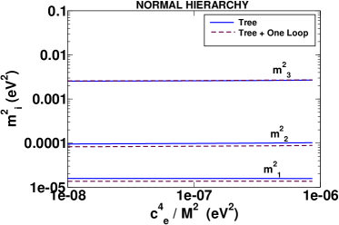
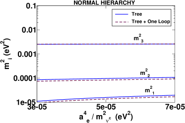
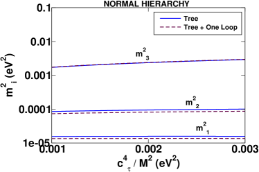
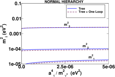
Figure 3: Neutrino mass squared values (mi2subscriptsuperscript𝑚2𝑖m^{2}_{i}) vs ci4M2subscriptsuperscript𝑐4𝑖superscript𝑀2\frac{c^{4}_{i}}{M^{2}} (left panel) and vs ai4mνc2subscriptsuperscript𝑎4𝑖subscriptsuperscript𝑚2superscript𝜈𝑐\frac{a^{4}_{i}}{m^{2}_{\nu^{c}}} (right panel) plots for the normal hierarchical pattern of light neutrino masses, i=e,μ,τ𝑖𝑒𝜇𝜏i=e,\mu,\tau.

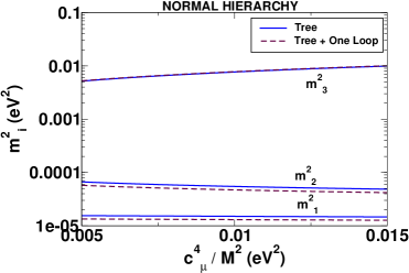
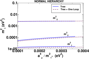
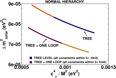
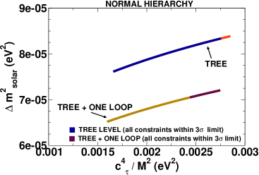
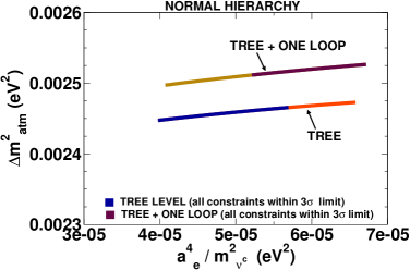
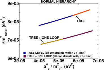
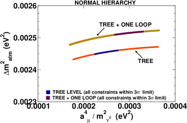
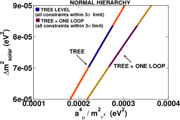
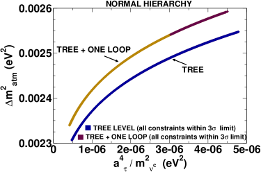
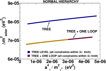
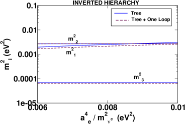
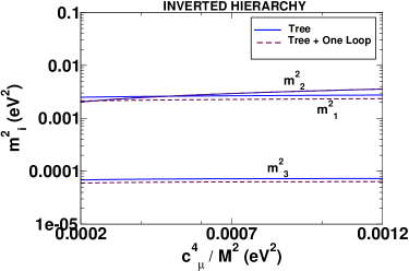
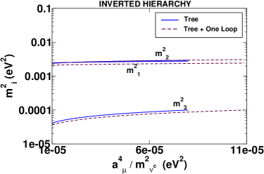
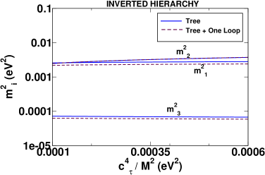
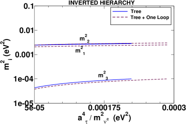
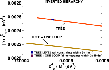
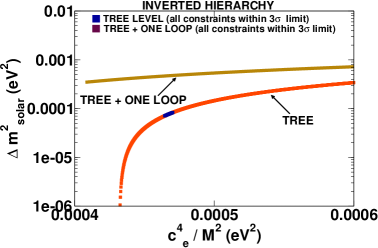
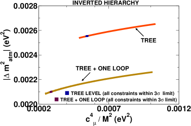
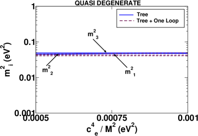
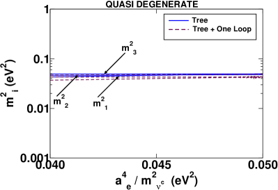
In the subsequent plots, we show the variation of the neutrino squared masses (mi2subscriptsuperscript𝑚2𝑖m^{2}_{i}) and the atmospheric and solar mass squared differences with the square of the seesaw parameters ci2Msubscriptsuperscript𝑐2𝑖𝑀\frac{c^{2}_{i}}{M} and ai2mνcsubscriptsuperscript𝑎2𝑖subscript𝑚superscript𝜈𝑐\frac{a^{2}_{i}}{m_{\nu^{c}}}. Results are shown for the tree level as well as the one-loop corrected neutrino masses. These plots also demonstrate the importance of one-loop corrections to neutrino masses compared to the tree level results.

Typical mass spectra are shown in figure 3. Note that a particular model parameter has been varied while the others are fixed at values given in tables 1 and 2. The effective light neutrino mass matrix given in eq.(18) suggests that as long as viYνiiv13λmuch-greater-thansubscriptsuperscript𝑣𝑖subscriptsuperscript𝑌𝑖𝑖𝜈subscript𝑣13𝜆v^{\prime}_{i}\gg\frac{Y^{ii}_{\nu}v_{1}}{3\lambda} and κλmuch-greater-than𝜅𝜆\kappa\gg\lambda, the second term on the right hand side of eq.(18) dominates over the first term and as a result the heaviest neutrino mass scale (m3subscript𝑚3m_{3}) is controlled mainly by the gaugino seesaw effect. This is because in this limit bicisubscript𝑏𝑖subscript𝑐𝑖b_{i}\approx c_{i}, and, as discussed earlier, a neutrino mass matrix with a structure (mν)ijcicjMsimilar-tosubscriptsubscript𝑚𝜈𝑖𝑗subscript𝑐𝑖subscript𝑐𝑗𝑀(m_{\nu})_{ij}\sim\frac{c_{i}c_{j}}{M} can produce only one non-zero neutrino mass. This feature is evident in figure3, where we see that m32subscriptsuperscript𝑚23m^{2}_{3} increases as a function of ci4/M2subscriptsuperscript𝑐4𝑖superscript𝑀2c^{4}_{i}/M^{2}. The other two masses are almost insensitive to ci2/Msubscriptsuperscript𝑐2𝑖𝑀c^{2}_{i}/M. A mild variation to m22subscriptsuperscript𝑚22m^{2}_{2} comes from the combined effect of gaugino and ordinary seesaw. On the other hand, the two lighter neutrino mass scales (m22subscriptsuperscript𝑚22m^{2}_{2} and m12subscriptsuperscript𝑚21m^{2}_{1}) are controlled predominantly by the ordinary seesaw parameters ai2/mνcsubscriptsuperscript𝑎2𝑖subscript𝑚superscript𝜈𝑐a^{2}_{i}/{m_{\nu^{c}}}. This behaviour is observed in the right panel figures of figure3. The heaviest neutrino mass scale is not much affected by the quantities ai2/mνcsubscriptsuperscript𝑎2𝑖subscript𝑚superscript𝜈𝑐a^{2}_{i}/{m_{\nu^{c}}}.

One can also see from these plots that the inclusion of one-loop corrections, for the chosen values of the soft SUSY breaking parameters, reduces the values of m22subscriptsuperscript𝑚22m^{2}_{2} and m12subscriptsuperscript𝑚21m^{2}_{1}, while increasing the value of m32subscriptsuperscript𝑚23m^{2}_{3} only mildly. This is because, with such a choice, the one-loop corrections cause partial cancellation in the generation of m1subscript𝑚1m_{1} and m2subscript𝑚2m_{2}. For the heaviest state, it is just the opposite, since the diagonalization of the tree-level mass matrix already yields a negative mass eigenvalue, on which the loop correction has an additive effect. If, with all other parameters fixed, the signs of λ𝜆\lambda and Aλsubscript𝐴𝜆A_{\lambda} are reversed (leading to a positive μ𝜇\mu in the place of a negative one), m1subscript𝑚1m_{1}, m2subscript𝑚2m_{2} and m3subscript𝑚3m_{3} are all found to decrease through loop corrections. A flip in the sign of κ𝜅\kappa and the corresponding soft breaking terms, on the other hand, causes a rise in all the mass eigenvalues, notably for m1subscript𝑚1m_{1} and m2subscript𝑚2m_{2}.

In the light of the discussion above, we now turn to explain the variation of Δmatm2Δsubscriptsuperscript𝑚2𝑎𝑡𝑚\Delta m^{2}_{atm} and Δmsolar2Δsubscriptsuperscript𝑚2𝑠𝑜𝑙𝑎𝑟\Delta m^{2}_{solar} with ci4/M2subscriptsuperscript𝑐4𝑖superscript𝑀2c^{4}_{i}/M^{2} and ai4/mνc2subscriptsuperscript𝑎4𝑖subscriptsuperscript𝑚2superscript𝜈𝑐a^{4}_{i}/{m^{2}_{\nu^{c}}} shown in figure4 and figure5. For our numerical analysis, in order to set the scale of the normal hierarchical spectrum, we choose m2|max<0.011eVevaluated-atsubscript𝑚2𝑚𝑎𝑥0.011eVm_{2}|_{max}<0.011~{}\rm{eV}. The left panel in figure4 shows that Δmatm2Δsubscriptsuperscript𝑚2𝑎𝑡𝑚\Delta m^{2}_{atm} increases more rapidly with cμ,τ4/M2subscriptsuperscript𝑐4𝜇𝜏superscript𝑀2c^{4}_{\mu,\tau}/M^{2}, whereas the variation with ce4/M2subscriptsuperscript𝑐4𝑒superscript𝑀2c^{4}_{e}/M^{2} is much slower as expected from figure3. Similar behaviour is shown for the one-loop corrected Δmatm2Δsubscriptsuperscript𝑚2𝑎𝑡𝑚\Delta m^{2}_{atm}. The small increase in the one-loop corrected result compared to the tree level one is essentially due to the splitting in m22subscriptsuperscript𝑚22m^{2}_{2} value as shown earlier. The variation of Δmsolar2Δsubscriptsuperscript𝑚2𝑠𝑜𝑙𝑎𝑟\Delta m^{2}_{solar} with ci4/M2subscriptsuperscript𝑐4𝑖superscript𝑀2c^{4}_{i}/M^{2} can be explained in a similar manner. Obviously, in this case the one-loop corrected result is smaller compared to the tree level one (see, figure3). However, one should note that Δmsolar2Δsubscriptsuperscript𝑚2𝑠𝑜𝑙𝑎𝑟\Delta m^{2}_{solar} falls off with cμ4/M2subscriptsuperscript𝑐4𝜇superscript𝑀2c^{4}_{\mu}/M^{2} as opposed to the variation with respect to the other two gaugino seesaw parameters. This is due to the fact that m22subscriptsuperscript𝑚22m^{2}_{2} slightly decreases with cμ4/M2subscriptsuperscript𝑐4𝜇superscript𝑀2c^{4}_{\mu}/M^{2} but show a slow increase with respect to ce4/M2subscriptsuperscript𝑐4𝑒superscript𝑀2c^{4}_{e}/M^{2} and cτ4/M2subscriptsuperscript𝑐4𝜏superscript𝑀2c^{4}_{\tau}/M^{2}. The dark solid lines in all these figures show the allowed values of various parameters where all the neutrino mass and mixing constraints are satisfied.
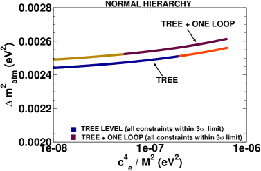
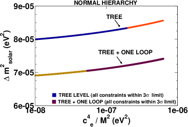
Refer to caption
Refer to caption
Refer to caption
Refer to caption
Refer to caption
Refer to caption
Figure 4: Atmospheric and solar mass squared differences (Δmatm2,Δmsolar2)Δsubscriptsuperscript𝑚2𝑎𝑡𝑚Δsubscriptsuperscript𝑚2𝑠𝑜𝑙𝑎𝑟(\Delta m^{2}_{atm},~{}\Delta m^{2}_{solar}) vs ci4M2subscriptsuperscript𝑐4𝑖superscript𝑀2\frac{c^{4}_{i}}{M^{2}} plots for the normal hierarchical pattern of light neutrino masses, i=e,μ,τ𝑖𝑒𝜇𝜏i=e,\mu,\tau. The full lines are shown for which only the constraints on Δmsolar2Δsubscriptsuperscript𝑚2𝑠𝑜𝑙𝑎𝑟\Delta m^{2}_{solar} is not within the 3σ𝜎\sigma limit. The dark coloured portions on these lines are the values of parameters for which all the neutrino constraints are within the 3σ𝜎\sigma limit. The red (yellow) coloured lines in the plots correspond to the tree (one-loop corrected) regions where all the constraints except Δmsolar2Δsubscriptsuperscript𝑚2𝑠𝑜𝑙𝑎𝑟\Delta m^{2}_{solar} are within 3σ𝜎\sigma allowed region. Other parameter choices are discussed in the text.
Refer to caption
Refer to caption
Refer to caption
Refer to caption
Refer to caption
Refer to caption
Figure 5: Atmospheric and solar mass squared differences (Δmatm2,Δmsolar2)Δsubscriptsuperscript𝑚2𝑎𝑡𝑚Δsubscriptsuperscript𝑚2𝑠𝑜𝑙𝑎𝑟(\Delta m^{2}_{atm},~{}\Delta m^{2}_{solar}) vs ai4/mνc2subscriptsuperscript𝑎4𝑖subscriptsuperscript𝑚2superscript𝜈𝑐a^{4}_{i}/m^{2}_{\nu^{c}} plots for the normal hierarchical pattern of light neutrino masses with i=e,μ,τ𝑖𝑒𝜇𝜏i=e,\mu,\tau. Colour specification is same as described in the context of figure 4. Other parameter choices are discussed in the text.

The variation of Δmatm2Δsubscriptsuperscript𝑚2𝑎𝑡𝑚\Delta m^{2}_{atm} and Δmsolar2Δsubscriptsuperscript𝑚2𝑠𝑜𝑙𝑎𝑟\Delta m^{2}_{solar} with ai4/mνc2subscriptsuperscript𝑎4𝑖subscriptsuperscript𝑚2superscript𝜈𝑐a^{4}_{i}/m^{2}_{\nu^{c}} in figure5 can be understood in a similar way by looking at the right panel plots of figure3. Δmatm2Δsubscriptsuperscript𝑚2𝑎𝑡𝑚\Delta m^{2}_{atm} shows a very little increase with ae,μ4/mνc2subscriptsuperscript𝑎4𝑒𝜇subscriptsuperscript𝑚2superscript𝜈𝑐a^{4}_{e,\mu}/m^{2}_{\nu^{c}} as expected, whereas the change is more rapid with aτ4/mνc2subscriptsuperscript𝑎4𝜏subscriptsuperscript𝑚2superscript𝜈𝑐a^{4}_{\tau}/m^{2}_{\nu^{c}} for the range of values considered along the x-axis. As in the case of figure4, the solid dark lines correspond to the allowed values of parameters where all the neutrino mass and mixing constraints are satisfied.
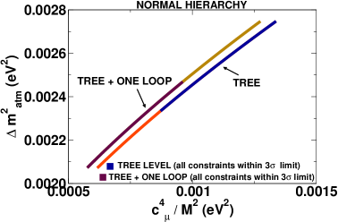
For higher values of ae,τ4/mνc2subscriptsuperscript𝑎4𝑒𝜏subscriptsuperscript𝑚2superscript𝜈𝑐a^{4}_{e,\tau}/m^{2}_{\nu^{c}}, m22subscriptsuperscript𝑚22m^{2}_{2} increases very slowly with these parameters (see, figure3) and this is reflected in the right panel plots of figure5, where Δmsolar2Δsubscriptsuperscript𝑚2𝑠𝑜𝑙𝑎𝑟\Delta m^{2}_{solar} shows a very slow variation with ae,τ4/mνc2subscriptsuperscript𝑎4𝑒𝜏subscriptsuperscript𝑚2superscript𝜈𝑐a^{4}_{e,\tau}/m^{2}_{\nu^{c}}. On the other hand, m22subscriptsuperscript𝑚22m^{2}_{2} increases more rapidly with aμ4/mνc2subscriptsuperscript𝑎4𝜇subscriptsuperscript𝑚2superscript𝜈𝑐a^{4}_{\mu}/m^{2}_{\nu^{c}}, giving rise to a faster variation of Δmsolar2Δsubscriptsuperscript𝑚2𝑠𝑜𝑙𝑎𝑟\Delta m^{2}_{solar}. The plots of figure5 show that larger values of Yukawa couplings are required in order to satisfy the global three flavour neutrino data, when one considers one-loop corrected neutrino mass matrix. However, there are allowed ranges of the parameters ai4/mνc2subscriptsuperscript𝑎4𝑖subscriptsuperscript𝑚2superscript𝜈𝑐a^{4}_{i}/m^{2}_{\nu^{c}}, where the neutrino data can be satisfied with both tree and one-loop corrected analysis.

We have also considered the variation of light neutrino mass squared differences with the effective bilinear RPsubscript𝑅𝑃R_{P} violating parameter, εi=Yijvjcsubscript𝜀𝑖superscript𝑌𝑖𝑗subscriptsuperscript𝑣𝑐𝑗\varepsilon_{i}=Y^{ij}v^{c}_{j}. For this particular numerical study we vary both Yνiisubscriptsuperscript𝑌𝑖𝑖𝜈Y^{ii}_{\nu} and the right handed sneutrino VEVs vicsubscriptsuperscript𝑣𝑐𝑖v^{c}_{i} simultaneously, in the suitable ranges around the values given in table 1 and 2. Δmatm2Δsubscriptsuperscript𝑚2𝑎𝑡𝑚\Delta m^{2}_{atm} is found to increase with εisubscript𝜀𝑖\varepsilon_{i}, whereas the solar mass squared difference decreases with increasing εisubscript𝜀𝑖\varepsilon_{i}. The 3σ3𝜎3\sigma allowed region for the solar and atmospheric mass squared differences were obtained for the lower values of εisubscript𝜀𝑖\varepsilon_{i}s. In addition, we have noticed that the correlations of Δmatm2Δsubscriptsuperscript𝑚2𝑎𝑡𝑚\Delta m^{2}_{atm} with εisubscript𝜀𝑖\varepsilon_{i} is sharper compared to the correlations seen in the case of Δmsolar2Δsubscriptsuperscript𝑚2𝑠𝑜𝑙𝑎𝑟\Delta m^{2}_{solar}.

Next let us discuss the dependence of Δmatm2Δsubscriptsuperscript𝑚2𝑎𝑡𝑚\Delta m^{2}_{atm} and Δmsolar2Δsubscriptsuperscript𝑚2𝑠𝑜𝑙𝑎𝑟\Delta m^{2}_{solar} on two specific model parameters, λ𝜆\lambda and κ𝜅\kappa, consistent with EWSB conditions. The loop corrections shift the allowed ranges of κ𝜅\kappa to lower values with some amount of overlap with the tree level result. On the other hand, the allowed ranges of λ𝜆\lambda shrinks towards higher values when one-loop corrections are included. These results are shown in figure6. We note in passing that the mass of the lightest CP-even scalar decreases with increasing λ𝜆\lambda. For example, λ=0.15𝜆0.15\lambda=0.15 can produce a lightest scalar mass of 40GeV40GeV40~{}\rm{GeV}, for suitable choices of other parameters. This happens because with increasing λ𝜆\lambda, the lightest scalar state picks up more and more right handed sneutrino admixture.
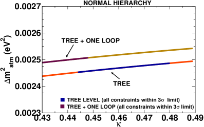
Refer to caption
Refer to caption
Refer to caption
Refer to caption
Figure 6: Plots showing the variations of Δmatm2,Δmsolar2Δsubscriptsuperscript𝑚2𝑎𝑡𝑚Δsubscriptsuperscript𝑚2𝑠𝑜𝑙𝑎𝑟\Delta m^{2}_{atm},~{}\Delta m^{2}_{solar} with model parameters λ𝜆\lambda and κ𝜅\kappa for normal hierarchy. Values of all other parameters are given by table 1 and 2. Colour specification is same as described in the context of figure 4. Other parameter choices are discussed in the text.

Finally, we will discuss the tanβtan𝛽\rm{tan}\beta dependence of Δmatm2Δsubscriptsuperscript𝑚2𝑎𝑡𝑚\Delta m^{2}_{atm} and Δmsolar2Δsubscriptsuperscript𝑚2𝑠𝑜𝑙𝑎𝑟\Delta m^{2}_{solar}. These plots are shown in figure 7. The quantity Δmatm2Δsubscriptsuperscript𝑚2𝑎𝑡𝑚\Delta m^{2}_{atm} decreases with the increasing values of tanβtan𝛽\rm{tan}\beta and nearly saturates for larger values of tanβtan𝛽\rm{tan}\beta. However, the one-loop corrected result for Δmatm2Δsubscriptsuperscript𝑚2𝑎𝑡𝑚\Delta m^{2}_{atm} is not much different from that at the tree level for a particular value of tanβ𝛽\tan\beta. On the other hand, the solar mass squared difference initially increases with tanβ𝛽\tan\beta and for higher values of tanβ𝛽\tan\beta the variation slows down and tends to saturate. The one-loop corrections result in lower values of Δmsolar2Δsubscriptsuperscript𝑚2𝑠𝑜𝑙𝑎𝑟\Delta m^{2}_{solar} for a particular tanβ𝛽\tan\beta. The darker and bigger points on both the plots of figure7 are the allowed values of tanβ𝛽\tan\beta, where all the neutrino experimental data are satisfied. Note that only a very small range of tanβ𝛽\tan\beta (similar-to\sim 10–14) is allowed. This is a very important observation of this analysis.
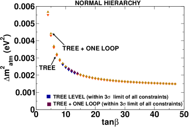
Refer to caption
Refer to caption
Figure 7: Δmatm2,Δmsolar2Δsubscriptsuperscript𝑚2𝑎𝑡𝑚Δsubscriptsuperscript𝑚2𝑠𝑜𝑙𝑎𝑟\Delta m^{2}_{atm},~{}\Delta m^{2}_{solar} vs tanβtan𝛽\rm{tan}\beta plots for the normal hierarchical pattern of light neutrino masses. The allowed values of tanβ𝛽\tan\beta are shown by bold points. Other parameter choices are shown in table 1 and 2.

Next we will discuss the light neutrino mixing and the effect of one-loop corrections on the mixing angles. It was shown in ref.[73] that for the normal hierarchical pattern of neutrino masses, when the parameter biaisimilar-tosubscript𝑏𝑖subscript𝑎𝑖b_{i}\sim a_{i}, the neutrino mixing angles θ23subscript𝜃23\theta_{23} and θ13subscript𝜃13\theta_{13} can be written as (with the tree level analysis),

sin2θ23bμ2bμ2+bτ2,superscript2subscript𝜃23subscriptsuperscript𝑏2𝜇subscriptsuperscript𝑏2𝜇subscriptsuperscript𝑏2𝜏\displaystyle\sin^{2}\theta_{23}\approx\frac{b^{2}_{\mu}}{b^{2}_{\mu}+b^{2}_{\tau}}, (54)

and

sin2θ13be2bμ2+bτ2.superscript2subscript𝜃13subscriptsuperscript𝑏2𝑒subscriptsuperscript𝑏2𝜇subscriptsuperscript𝑏2𝜏\displaystyle\sin^{2}\theta_{13}\approx\frac{b^{2}_{e}}{b^{2}_{\mu}+b^{2}_{\tau}}. (55)

On the other hand, the mixing angle θ12subscript𝜃12\theta_{12} is a much more complicated function of the parameters bisubscript𝑏𝑖b_{i} and aisubscript𝑎𝑖a_{i} and we do not show it here. Now, when biaisimilar-tosubscript𝑏𝑖subscript𝑎𝑖b_{i}\sim a_{i}, we can easily see from eq.(14), that

viYνiiv13λ(tanβ1).similar-tosubscriptsuperscript𝑣𝑖subscriptsuperscript𝑌𝑖𝑖𝜈subscript𝑣13𝜆𝛽1\displaystyle v^{\prime}_{i}\sim\frac{Y^{ii}_{\nu}v_{1}}{3\lambda}(\tan\beta-1). (56)

This implies that for tanβmuch-greater-than𝛽absent\tan\beta\gg 1 (recall that the allowed range of tanβ𝛽\tan\beta is similar-to\sim 10–14),

viYνiiv13λ.much-greater-thansubscriptsuperscript𝑣𝑖subscriptsuperscript𝑌𝑖𝑖𝜈subscript𝑣13𝜆\displaystyle v^{\prime}_{i}\gg\frac{Y^{ii}_{\nu}v_{1}}{3\lambda}. (57)

As we have discussed earlier, for such values of visubscriptsuperscript𝑣𝑖v^{\prime}_{i}, the quantities bicisubscript𝑏𝑖subscript𝑐𝑖b_{i}\approx c_{i}. Hence, the mixing angles θ23subscript𝜃23\theta_{23} and θ13subscript𝜃13\theta_{13} can be approximately written as

sin2θ23cμ2cμ2+cτ2,superscript2subscript𝜃23subscriptsuperscript𝑐2𝜇subscriptsuperscript𝑐2𝜇subscriptsuperscript𝑐2𝜏\displaystyle\sin^{2}\theta_{23}\approx\frac{c^{2}_{\mu}}{c^{2}_{\mu}+c^{2}_{\tau}}, (58)

and

sin2θ13ce2cμ2+cτ2.superscript2subscript𝜃13subscriptsuperscript𝑐2𝑒subscriptsuperscript𝑐2𝜇subscriptsuperscript𝑐2𝜏\displaystyle\sin^{2}\theta_{13}\approx\frac{c^{2}_{e}}{c^{2}_{\mu}+c^{2}_{\tau}}. (59)

Naively, one would also expect that sin2θ12superscript2subscript𝜃12\sin^{2}\theta_{12} should show some correlation with the quantity ce2/cμ2subscriptsuperscript𝑐2𝑒subscriptsuperscript𝑐2𝜇c^{2}_{e}/c^{2}_{\mu}. However, as mentioned earlier, this is a very simple minded expectation since sin2θ12superscript2subscript𝜃12\sin^{2}\theta_{12} has a more complicated dependence on the model parameters.

The variation of all three mixing angles with the corresponding parameters are shown in figure8. Note that in order to generate these plots, we vary only the quantities cisubscript𝑐𝑖c_{i} and all the other parameters are fixed at the values given in tables 1 and 2. We have chosen the range of parameters in such a way that the 3-flavour global neutrino data are satisfied. The mixing angles have been calculated numerically by diagonalizing the neutrino mass matrix in eq.(18) and in eq.(39). As expected from our approximate analytical expressions, these plots show very nice correlations of the mixing angles θ23subscript𝜃23\theta_{23} and θ13subscript𝜃13\theta_{13} with the relevant parameters as discussed in eqs.(58) and (59). For example, note that when cμcτsubscript𝑐𝜇subscript𝑐𝜏c_{\mu}\approx c_{\tau}, sin2θ23superscript2subscript𝜃23\sin^{2}\theta_{23} is predicted to be \approx 0.5 and that is what we observe in the tree level plot in figure8. However, when one-loop corrections are considered, the value of sin2θ23superscript2subscript𝜃23\sin^{2}\theta_{23} is predicted to be somewhat on the lower side of the 3σ𝜎\sigma allowed region. This can be understood by looking at the left panel plots of figure4, where one can see that the one-loop corrected results prefer lower values of cμ2subscriptsuperscript𝑐2𝜇c^{2}_{\mu} and higher values of cτ2subscriptsuperscript𝑐2𝜏c^{2}_{\tau}. Obviously, this gives smaller sin2θ23superscript2subscript𝜃23\sin^{2}\theta_{23}. On the other hand, the tree level analysis prefers higher values of cμ2subscriptsuperscript𝑐2𝜇c^{2}_{\mu} and both lower and higher values of cτ2subscriptsuperscript𝑐2𝜏c^{2}_{\tau}. This gives rise to large as well as small values of sin2θ23superscript2subscript𝜃23\sin^{2}\theta_{23}.

Refer to caption
Refer to caption
Refer to caption
Figure 8: Variation of sin2θ23superscriptsin2subscript𝜃23\rm{sin}^{2}\theta_{23} with cμ2(cμ2+cτ2)subscriptsuperscript𝑐2𝜇subscriptsuperscript𝑐2𝜇subscriptsuperscript𝑐2𝜏\frac{c^{2}_{\mu}}{(c^{2}_{\mu}+c^{2}_{\tau})}, sin2θ12superscriptsin2subscript𝜃12\rm{sin}^{2}\theta_{12} with ce2cμ2subscriptsuperscript𝑐2𝑒subscriptsuperscript𝑐2𝜇\frac{c^{2}_{e}}{c^{2}_{\mu}}, sin2θ13superscriptsin2subscript𝜃13\rm{sin}^{2}\theta_{13} with ce2(cμ2+cτ2)subscriptsuperscript𝑐2𝑒subscriptsuperscript𝑐2𝜇subscriptsuperscript𝑐2𝜏\frac{c^{2}_{e}}{(c^{2}_{\mu}+c^{2}_{\tau})} for normal hierarchy of light neutrino masses. Other parameter choices are discussed in the text.

If one looks at the plot of sin2θ13superscript2subscript𝜃13\sin^{2}\theta_{13} in figure 8, then it is evident that the amount νesubscript𝜈𝑒\nu_{e} flavour in the heaviest state (ν3)subscript𝜈3(\nu_{3}) decreases a little bit with the inclusion of one-loop corrections for a fixed value of the quantity ce2(cμ2+cτ2)subscriptsuperscript𝑐2𝑒subscriptsuperscript𝑐2𝜇subscriptsuperscript𝑐2𝜏\frac{c^{2}_{e}}{(c^{2}_{\mu}+c^{2}_{\tau})}. Very small sin2θ13superscript2subscript𝜃13\sin^{2}\theta_{13} demands ce2cμ2,cτ2much-less-thansubscriptsuperscript𝑐2𝑒subscriptsuperscript𝑐2𝜇subscriptsuperscript𝑐2𝜏c^{2}_{e}\ll c^{2}_{\mu},~{}c^{2}_{\tau}. This feature is also consistent with the plots in figure4. The correlation of sin2θ12superscript2subscript𝜃12\sin^{2}\theta_{12} with the ratio ce2/cμ2subscriptsuperscript𝑐2𝑒subscriptsuperscript𝑐2𝜇c^{2}_{e}/c^{2}_{\mu} is not very sharp as expected from the discussion given above. However, a large θ12subscript𝜃12\theta_{12} mixing angle requires a larger value of this ratio. The effect of one-loop correction is more pronounced in this case and predicts a smaller value of sin2θ12superscript2subscript𝜃12\sin^{2}\theta_{12} compared to the tree level result. There is no specific correlation of the mixing angles with the quantities ai2subscriptsuperscript𝑎2𝑖a^{2}_{i} and we do not show them here.

4.2 Inverted hierarchy

In this subsection we perform a similar numerical analysis for the inverted hierarchical scheme of three light neutrino masses. Recall that for the inverted hierarchical pattern of light neutrino masses, the absolute values of the mass eigenvalues are such that m2>m1m3subscript𝑚2subscript𝑚1much-greater-thansubscript𝑚3m_{2}>m_{1}\gg m_{3}. Thus the solar and the atmospheric mass squared differences are defined as Δmatm2=m12m32Δsubscriptsuperscript𝑚2𝑎𝑡𝑚subscriptsuperscript𝑚21subscriptsuperscript𝑚23\Delta m^{2}_{atm}=m^{2}_{1}-m^{2}_{3} and Δmsolar2=m22m12Δsubscriptsuperscript𝑚2𝑠𝑜𝑙𝑎𝑟subscriptsuperscript𝑚22subscriptsuperscript𝑚21\Delta m^{2}_{solar}=m^{2}_{2}-m^{2}_{1}. In order to generate such a mass pattern, the choices of neutrino Yukawa couplings Yνiisuperscriptsubscript𝑌𝜈𝑖𝑖Y_{\nu}^{ii} and the left-handed sneutrino VEVs visubscriptsuperscript𝑣𝑖v^{\prime}_{i} are shown in table 2. However, these are just sample choices and other choices also exist as we will see during the course of this discussion. The choices of other parameters are shown in table 1. The effect of one-loop corrections to the mass eigenvalues are such that the absolute values of masses m3subscript𝑚3m_{3} and m1subscript𝑚1m_{1} become smaller whereas m2subscript𝑚2m_{2} grows in magnitude. This effect of increasing the absolute value of m2subscript𝑚2m_{2} while decreasing that of m1subscript𝑚1m_{1} makes it extremely difficult to account for the present 3σ𝜎\sigma limits on Δmsolar2Δsubscriptsuperscript𝑚2𝑠𝑜𝑙𝑎𝑟\Delta m^{2}_{solar}.

Refer to caption
Refer to caption
Refer to caption
Refer to caption
Refer to caption
Refer to caption
Figure 9: Neutrino mass squared values (mi2subscriptsuperscript𝑚2𝑖m^{2}_{i}) vs ci4M2subscriptsuperscript𝑐4𝑖superscript𝑀2\frac{c^{4}_{i}}{M^{2}} (left panel) and vs ai4mνc2subscriptsuperscript𝑎4𝑖subscriptsuperscript𝑚2superscript𝜈𝑐\frac{a^{4}_{i}}{m^{2}_{\nu^{c}}} (right panel) plots for the inverted hierarchical pattern of light neutrino masses, i=e,μ,τ𝑖𝑒𝜇𝜏i=e,\mu,\tau.

Typical mass spectra are shown in figure 9. Once again note that a particular model parameter has been varied while the others are fixed at values given in tables 1 and 2. As it is evident from these plots, the masses m1subscript𝑚1m_{1} and m3subscript𝑚3m_{3} are controlled mainly by the parameters ai2/mνcsubscriptsuperscript𝑎2𝑖superscriptsubscript𝑚𝜈𝑐a^{2}_{i}/m_{\nu}^{c}, whereas the mass m2subscript𝑚2m_{2} is controlled by the seesaw parameters ci2/Msubscriptsuperscript𝑐2𝑖𝑀c^{2}_{i}/M though there is a small contribution coming from ai2/mνcsubscriptsuperscript𝑎2𝑖superscriptsubscript𝑚𝜈𝑐a^{2}_{i}/m_{\nu}^{c} as well.

Let us now turn our attention to the variation of |Δmatm2|Δsubscriptsuperscript𝑚2𝑎𝑡𝑚|\Delta m^{2}_{atm}| and Δmsolar2Δsubscriptsuperscript𝑚2𝑠𝑜𝑙𝑎𝑟\Delta m^{2}_{solar} with ci4/M2subscriptsuperscript𝑐4𝑖superscript𝑀2c^{4}_{i}/M^{2} and ai4/mνc2subscriptsuperscript𝑎4𝑖subscriptsuperscript𝑚2superscript𝜈𝑐a^{4}_{i}/{m^{2}_{\nu^{c}}} shown in figure 10 and figure 11. For our numerical analysis, we have set the scale of m3subscript𝑚3m_{3} as |m3|<0.011eVsubscript𝑚30.011eV|m_{3}|<0.011~{}\rm{eV}. The left panel in figure 10 shows that |Δmatm2|Δsubscriptsuperscript𝑚2𝑎𝑡𝑚|\Delta m^{2}_{atm}| increases with cμ,τ4/M2subscriptsuperscript𝑐4𝜇𝜏superscript𝑀2c^{4}_{\mu,\tau}/M^{2} and decreases with ce4/M2subscriptsuperscript𝑐4𝑒superscript𝑀2c^{4}_{e}/M^{2}. This is essentially the behaviour shown by m12subscriptsuperscript𝑚21m^{2}_{1} with the variation of ci4/M2subscriptsuperscript𝑐4𝑖superscript𝑀2c^{4}_{i}/M^{2}. Similar behaviour is obtained for the one-loop corrected Δmatm2Δsubscriptsuperscript𝑚2𝑎𝑡𝑚\Delta m^{2}_{atm}. The decrease in the one-loop corrected result compared to the tree level one is due to the splitting in m12subscriptsuperscript𝑚21m^{2}_{1} value as shown in figure9.

Refer to caption
Refer to caption
Refer to caption
Refer to caption
Refer to caption
Refer to caption
Figure 10: Atmospheric and solar mass squared differences (|Δmatm2|,Δmsolar2)Δsubscriptsuperscript𝑚2𝑎𝑡𝑚Δsubscriptsuperscript𝑚2𝑠𝑜𝑙𝑎𝑟(|\Delta m^{2}_{atm}|,~{}\Delta m^{2}_{solar}) vs ci4M2superscriptsubscript𝑐𝑖4superscript𝑀2\frac{c_{i}^{4}}{M^{2}} plots for the inverted hierarchical pattern of light neutrino masses with i=e,μ,τ𝑖𝑒𝜇𝜏i=e,\mu,\tau. Colour specification is same as described in the context of figure 4. Choices of other parameters are discussed in the text.

The variation of Δmsolar2Δsubscriptsuperscript𝑚2𝑠𝑜𝑙𝑎𝑟\Delta m^{2}_{solar} with ci4/M2subscriptsuperscript𝑐4𝑖superscript𝑀2c^{4}_{i}/M^{2} can be understood in a similar manner by looking at figure9. As explained earlier, in the case of Δmsolar2Δsubscriptsuperscript𝑚2𝑠𝑜𝑙𝑎𝑟\Delta m^{2}_{solar}, the one-loop corrected result is larger compared to the tree level one. The range of parameters satisfying all the three flavour global neutrino data are shown by the fewer dark points on the plots. Note that the increase of Δmsolar2Δsubscriptsuperscript𝑚2𝑠𝑜𝑙𝑎𝑟\Delta m^{2}_{solar} at the one-loop level is such that we do not even see any allowed range of parameters when looking at the variation with respect to ce,τ4/M2subscriptsuperscript𝑐4𝑒𝜏superscript𝑀2c^{4}_{e,\tau}/M^{2}. Once again, the behaviour of |Δmatm2|Δsubscriptsuperscript𝑚2𝑎𝑡𝑚|\Delta m^{2}_{atm}| and Δmsolar2Δsubscriptsuperscript𝑚2𝑠𝑜𝑙𝑎𝑟\Delta m^{2}_{solar} with the change in the parameters ai4/mνc2subscriptsuperscript𝑎4𝑖subscriptsuperscript𝑚2superscript𝜈𝑐a^{4}_{i}/m^{2}_{\nu^{c}} (shown in figure11) can be explained by looking at the right panel plots of figure9.
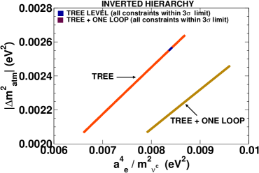
Refer to caption
Refer to caption
Refer to caption
Refer to caption
Refer to caption
Refer to caption
Figure 11: Atmospheric and solar mass squared differences (|Δmatm2|,Δmsolar2)Δsubscriptsuperscript𝑚2𝑎𝑡𝑚Δsubscriptsuperscript𝑚2𝑠𝑜𝑙𝑎𝑟(|\Delta m^{2}_{atm}|,~{}\Delta m^{2}_{solar}) vs ai4/mνc2subscriptsuperscript𝑎4𝑖subscriptsuperscript𝑚2superscript𝜈𝑐a^{4}_{i}/m^{2}_{\nu^{c}} plots for the inverted hierarchical pattern of light neutrino masses with i=e,μ,τ𝑖𝑒𝜇𝜏i=e,\mu,\tau. Colour specification is same as described in the context of figure 4. Choices of other parameters are discussed in the text.

We have also investigated the nature of variation of |Δmatm2|Δsubscriptsuperscript𝑚2𝑎𝑡𝑚|\Delta m^{2}_{atm}| and Δmsolar2Δsubscriptsuperscript𝑚2𝑠𝑜𝑙𝑎𝑟\Delta m^{2}_{solar} with εi2subscriptsuperscript𝜀2𝑖\varepsilon^{2}_{i}, the squared effective bilinear RPsubscript𝑅𝑃R_{P}-violating parameters. |Δmatm2|Δsubscriptsuperscript𝑚2𝑎𝑡𝑚|\Delta m^{2}_{atm}| was found to increase with εi2subscriptsuperscript𝜀2𝑖\varepsilon^{2}_{i} (the increase is sharper for ε12subscriptsuperscript𝜀21\varepsilon^{2}_{1}), whereas Δmsolar2Δsubscriptsuperscript𝑚2𝑠𝑜𝑙𝑎𝑟\Delta m^{2}_{solar} initially increases very sharply with εi2subscriptsuperscript𝜀2𝑖\varepsilon^{2}_{i} (particularly for ε12subscriptsuperscript𝜀21\varepsilon^{2}_{1} and ε22subscriptsuperscript𝜀22\varepsilon^{2}_{2}) and then becomes flat. In the one-loop corrected results we do not find any range of values for parameters where the neutrino data are satisfied.

The variation of mass squared differences with λ𝜆\lambda and κ𝜅\kappa have also been analyzed. The variation of |Δmatm2|Δsubscriptsuperscript𝑚2𝑎𝑡𝑚|\Delta m^{2}_{atm}| and Δmsolar2Δsubscriptsuperscript𝑚2𝑠𝑜𝑙𝑎𝑟\Delta m^{2}_{solar} with λ𝜆\lambda and κ𝜅\kappa are found to be opposite to those of normal hierarchical scenario. The one-loop corrected results do not show any allowed ranges of λ𝜆\lambda and κ𝜅\kappa (for the chosen values of other parameters) where the neutrino data can be satisfied.
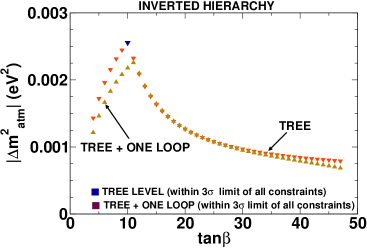
The tanβ𝛽\tan\beta dependence of |Δmatm2|Δsubscriptsuperscript𝑚2𝑎𝑡𝑚|\Delta m^{2}_{atm}| and Δmsolar2Δsubscriptsuperscript𝑚2𝑠𝑜𝑙𝑎𝑟\Delta m^{2}_{solar} is shown in figure12. One can see from these two figures that |Δmatm2|Δsubscriptsuperscript𝑚2𝑎𝑡𝑚|\Delta m^{2}_{atm}| initially increases and then starts decreasing at a value of tanβ𝛽\tan\beta around 101010. On the other hand, Δmsolar2Δsubscriptsuperscript𝑚2𝑠𝑜𝑙𝑎𝑟\Delta m^{2}_{solar} initially decreases and then starts increasing around the same value of tanβ𝛽\tan\beta. Note that the one-loop corrected result for |Δmatm2|Δsubscriptsuperscript𝑚2𝑎𝑡𝑚|\Delta m^{2}_{atm}| is lower than the corresponding tree level result for tanβ<10𝛽10\tan\beta<10 whereas the one-loop corrected result for Δmsolar2Δsubscriptsuperscript𝑚2𝑠𝑜𝑙𝑎𝑟\Delta m^{2}_{solar} is lower than the corresponding tree level result for tanβ>10𝛽10\tan\beta>10. For the chosen values of other parameters we see that the one-loop corrected analysis does not provide any value of tanβ𝛽\tan\beta where the neutrino data can be satisfied.
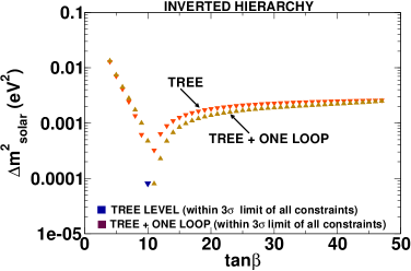
Refer to caption
Refer to caption
Figure 12: |Δmatm2|,Δmsolar2Δsubscriptsuperscript𝑚2𝑎𝑡𝑚Δsubscriptsuperscript𝑚2𝑠𝑜𝑙𝑎𝑟|\Delta m^{2}_{atm}|,~{}\Delta m^{2}_{solar} vs tanβtan𝛽\rm{tan}\beta plots for the inverted hierarchical pattern of light neutrino masses. Choices of other parameters are discussed in the text.

We conclude the discussion on inverted hierarchy by addressing the dependence of neutrino mixing angles with the relevant parameters. In figure13 we show the variation of the neutrino mixing angles with the same set of parameters as chosen for the normal hierarchical scenario. We notice that for inverted hierarchy the quantity sin2θ23superscript2subscript𝜃23\sin^{2}\theta_{23} decreases with increasing cμ2(cμ2+cτ2)subscriptsuperscript𝑐2𝜇subscriptsuperscript𝑐2𝜇subscriptsuperscript𝑐2𝜏\frac{c^{2}_{\mu}}{(c^{2}_{\mu}+c^{2}_{\tau})} which is just opposite to that of the normal hierarchy (see, figure8). Nevertheless, the correlation of sin2θ23superscript2subscript𝜃23\sin^{2}\theta_{23} with cμ2(cμ2+cτ2)subscriptsuperscript𝑐2𝜇subscriptsuperscript𝑐2𝜇subscriptsuperscript𝑐2𝜏\frac{c^{2}_{\mu}}{(c^{2}_{\mu}+c^{2}_{\tau})} is as sharp as in the case of normal hierarchy. A similar feature is obtained for the variation with aμ2(aμ2+aτ2)subscriptsuperscript𝑎2𝜇subscriptsuperscript𝑎2𝜇subscriptsuperscript𝑎2𝜏\frac{a^{2}_{\mu}}{(a^{2}_{\mu}+a^{2}_{\tau})}.

On the other hand, the correlations of sin2θ12superscript2subscript𝜃12\sin^{2}\theta_{12} with ce2cμ2subscriptsuperscript𝑐2𝑒subscriptsuperscript𝑐2𝜇\frac{c^{2}_{e}}{c^{2}_{\mu}} and ae2aμ2subscriptsuperscript𝑎2𝑒subscriptsuperscript𝑎2𝜇\frac{a^{2}_{e}}{a^{2}_{\mu}} and the correlations of sin2θ13superscript2subscript𝜃13\sin^{2}\theta_{13} with ce2(cμ2+cτ2)subscriptsuperscript𝑐2𝑒subscriptsuperscript𝑐2𝜇subscriptsuperscript𝑐2𝜏\frac{c^{2}_{e}}{(c^{2}_{\mu}+c^{2}_{\tau})} and ae2(aμ2+aτ2)subscriptsuperscript𝑎2𝑒subscriptsuperscript𝑎2𝜇subscriptsuperscript𝑎2𝜏\frac{a^{2}_{e}}{(a^{2}_{\mu}+a^{2}_{\tau})} are not very sharp and we do not show them here. There are allowed values of relevant parameters where all neutrino data can be satisfied. Remember that, for the plots with cisubscript𝑐𝑖c_{i}s, we varied all the cisubscript𝑐𝑖c_{i}s simultaneously, keeping the values of aisubscript𝑎𝑖a_{i}s fixed at the ones determined by the parameters in table 2. Similarly, for the variation of aisubscript𝑎𝑖a_{i}s, the quantities cisubscript𝑐𝑖c_{i}s were fixed. The inclusion of one-loop corrections restrict the allowed values of parameter points significantly compared to the tree level results.
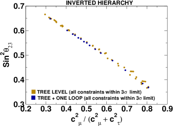
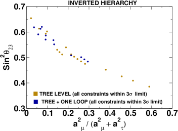
Refer to caption
Refer to caption
Figure 13: Variation of sin2θ23superscript2subscript𝜃23\sin^{2}\theta_{23} with cμ2(cμ2+cτ2)subscriptsuperscript𝑐2𝜇subscriptsuperscript𝑐2𝜇subscriptsuperscript𝑐2𝜏\frac{c^{2}_{\mu}}{(c^{2}_{\mu}+c^{2}_{\tau})} and aμ2(aμ2+aτ2)subscriptsuperscript𝑎2𝜇subscriptsuperscript𝑎2𝜇subscriptsuperscript𝑎2𝜏\frac{a^{2}_{\mu}}{(a^{2}_{\mu}+a^{2}_{\tau})} for inverted hierarchy of light neutrino masses. Choices of other parameters are discussed in the text.

4.3 Quasi-degenerate spectra

The discussion on the light neutrino mass spectrum remains incomplete without a note on the so-called “quasi-degenerate” scenario. A truly degenerate scenario of three light neutrino masses is, however, inconsistent with the oscillation data (see eq.(LABEL:oscillation-data)). Hence, the quasi-degenerate scenario of light neutrino masses is defined in such a way that in this case all the three individual neutrino masses are much larger compared to the atmospheric neutrino mass scale. Mathematically, one writes m1m2m3|Δmatm2|subscript𝑚1subscript𝑚2subscript𝑚3much-greater-thanΔsubscriptsuperscript𝑚2𝑎𝑡𝑚m_{1}\approx m_{2}\approx m_{3}\gg\sqrt{|\Delta m^{2}_{atm}|}. Obviously, the oscillation data suggest that even in such a situation there must be a mild hierarchy among the degenerate neutrinos.

In this section we have shown that the huge parameter space of μν𝜇𝜈\mu\nuSSM always leaves us with enough room to accommodate quasi-degenerate spectrum. For our numerical analysis, we called a set of light neutrino masses to be quasi-degenerate if the lightest among them is greater than 0.1 eV. We choose two sets of sample parameter points which are shown in table 3 (values of other parameters are same as in table 1). For these two sets of neutrino Yukawa couplings (Yνiisuperscriptsubscript𝑌𝜈𝑖𝑖Y_{\nu}^{ii}) and the left-handed sneutrino VEVs (visubscriptsuperscript𝑣𝑖v^{\prime}_{i}) we observe the following patterns of light neutrino masses at the tree level

(i) Quasi-degenerate-I: m3>m2>m1|Δmatm2|,fragmentsfragmentssimilar-tosubscript𝑚3subscript𝑚2fragmentsfragmentssimilar-tosubscript𝑚1much-greater-thanΔsubscriptsuperscript𝑚2𝑎𝑡𝑚m_{3}\mathrel{\mathchoice{\vbox{\offinterlineskip\halign{$\m@th\displaystyle\hfil#\hfil$\cr>\crcr\sim\crcr} }}{\vbox{\offinterlineskip\halign{$\m@th\textstyle\hfil#\hfil$\cr>\crcr\sim\crcr} }}{\vbox{\offinterlineskip\halign{$\m@th\scriptstyle\hfil#\hfil$\cr>\crcr\sim\crcr} }}{\vbox{\offinterlineskip\halign{$\m@th\scriptscriptstyle\hfil#\hfil$\cr>\crcr\sim\crcr} }}}m_{2}\mathrel{\mathchoice{\vbox{\offinterlineskip\halign{$\m@th\displaystyle\hfil#\hfil$\cr>\crcr\sim\crcr} }}{\vbox{\offinterlineskip\halign{$\m@th\textstyle\hfil#\hfil$\cr>\crcr\sim\crcr} }}{\vbox{\offinterlineskip\halign{$\m@th\scriptstyle\hfil#\hfil$\cr>\crcr\sim\crcr} }}{\vbox{\offinterlineskip\halign{$\m@th\scriptscriptstyle\hfil#\hfil$\cr>\crcr\sim\crcr} }}}m_{1}\gg\sqrt{|\Delta m^{2}_{atm}|},
(ii) Quasi-degenerate-II: m2>m1>m3|Δmatm2|.fragmentsfragmentssimilar-tosubscript𝑚2subscript𝑚1fragmentsfragmentssimilar-tosubscript𝑚3much-greater-thanΔsubscriptsuperscript𝑚2𝑎𝑡𝑚m_{2}\mathrel{\mathchoice{\vbox{\offinterlineskip\halign{$\m@th\displaystyle\hfil#\hfil$\cr>\crcr\sim\crcr} }}{\vbox{\offinterlineskip\halign{$\m@th\textstyle\hfil#\hfil$\cr>\crcr\sim\crcr} }}{\vbox{\offinterlineskip\halign{$\m@th\scriptstyle\hfil#\hfil$\cr>\crcr\sim\crcr} }}{\vbox{\offinterlineskip\halign{$\m@th\scriptscriptstyle\hfil#\hfil$\cr>\crcr\sim\crcr} }}}m_{1}\mathrel{\mathchoice{\vbox{\offinterlineskip\halign{$\m@th\displaystyle\hfil#\hfil$\cr>\crcr\sim\crcr} }}{\vbox{\offinterlineskip\halign{$\m@th\textstyle\hfil#\hfil$\cr>\crcr\sim\crcr} }}{\vbox{\offinterlineskip\halign{$\m@th\scriptstyle\hfil#\hfil$\cr>\crcr\sim\crcr} }}{\vbox{\offinterlineskip\halign{$\m@th\scriptscriptstyle\hfil#\hfil$\cr>\crcr\sim\crcr} }}}m_{3}\gg\sqrt{|\Delta m^{2}_{atm}|}.

For case (i), we have varied the parameters around the values in table 3 and identified a few extremely fine-tuned points in the parameter space where either the tree level or the one-loop corrected result is consistent with the three flavour global neutrino data. Two representative spectrum as function of ce4M2subscriptsuperscript𝑐4𝑒superscript𝑀2\frac{c^{4}_{e}}{M^{2}} and ae4mνc2subscriptsuperscript𝑎4𝑒subscriptsuperscript𝑚2superscript𝜈𝑐\frac{a^{4}_{e}}{m^{2}_{\nu^{c}}} are shown in figure 14.

Refer to caption
Refer to caption
Figure 14: Neutrino mass squared values (mi2subscriptsuperscript𝑚2𝑖m^{2}_{i}) vs ce4M2subscriptsuperscript𝑐4𝑒superscript𝑀2\frac{c^{4}_{e}}{M^{2}} (left panel) and vs ae4mνc2subscriptsuperscript𝑎4𝑒subscriptsuperscript𝑚2superscript𝜈𝑐\frac{a^{4}_{e}}{m^{2}_{\nu^{c}}} (right panel) plots for the quasi-degenerate pattern of light neutrino masses.
Yνii×107subscriptsuperscript𝑌𝑖𝑖𝜈superscript107Y^{ii}_{\nu}\times 10^{7} vi×105(GeV)subscriptsuperscript𝑣𝑖superscript105GeVv^{\prime}_{i}\times 10^{5}(\rm{GeV})
Yν11subscriptsuperscript𝑌11𝜈Y^{11}_{\nu} Yν22subscriptsuperscript𝑌22𝜈Y^{22}_{\nu} Yν33subscriptsuperscript𝑌33𝜈Y^{33}_{\nu} v1subscriptsuperscript𝑣1v^{\prime}_{1} v2subscriptsuperscript𝑣2v^{\prime}_{2} v3subscriptsuperscript𝑣3v^{\prime}_{3}
Quasi-degenerate-I 19.60 19.94 19.99 9.75 10.60 11.83
Quasi-degenerate-II 18.50 18.00 18.00 9.85 10.50 10.10
Table 3: Values of neutrino Yukawa couplings and left handed sneutrino VEVs, used as sample parameter points to obtain quasi-degenerate light neutrino spectrum. Around these values, the corresponding parameters were varied for the plots shown in figure 14.

As mentioned earlier, one can play with the model parameters and obtain a spectrum with a different ordering of masses termed as “Quasi-degenerate-II” in table 3. However, for such an ordering of masses, we found that it was rather impossible to find any region of parameter space where the one-loop corrected result satisfies all the constraints on neutrino masses and mixing. Nevertheless, we must emphasize here that it is not a completely generic conclusion and for other choices of soft SUSY breaking and other parameters it could be possible to have a spectrum like that shown in “Quasi degenerate II” with neutrino constraints satisfied even at the one-loop level. On the other hand, there exists regions where neutrino data are satisfied at the tree level with this ordering of masses.

5 Summary and Conclusion

In this paper, we have performed a systematic study of neutrino masses and mixing in a non-minimal extension of the MSSM, known as μν𝜇𝜈\mu\nuSSM, with the complete set of one-loop radiative corrections, over and above the effects from the seesaw mechanism (of Types I and III). A set of right chiral neutrino superfields, introduced in this model provide a solution to the μ𝜇\mu-problem. Lepton number is broken by one ΔLΔ𝐿\Delta L = 1 term comprising the right-chiral neutrinos and the Higgs superfields and another ΔLΔ𝐿\Delta L = 3 term involving only the right chiral neutrinos in the superpotential. The corresponding soft SUSY breaking terms in the scalar potential together with the F-term contribution from the superpotential, induce VEVs of sneutrinos of both right and left chirality. The right chiral neutrinos, together with neutralinos, are instrumental in the generation of light neutrino masses at the tree level.

In [73], where a tree-level analysis of neutrino masses and mixing was carried out, it was shown that tree level masses could be generated in this fashion for all three light neutrinos, even with a flavour diagonal structure of neutrino Yukawa couplings (Yνijsuperscriptsubscript𝑌𝜈𝑖𝑗Y_{\nu}^{ij}). In this work we have improved the analysis with the inclusion of one-loop radiative corrections, for various patterns of light neutrino masses, namely, the normal, inverted and quasi-degenerate spectra, Attempts have been made to identify regions in the SUSY parameter space, which can accommodate the three patterns in turn. Our analysis clearly shows that the multi-dimensional parameter space of μν𝜇𝜈\mu\nuSSM leaves enough room to accommodate all the diverse mass hierarchies of the three active light neutrinos.

As a prerequisite of the loop calculation, we have derived the entire set of Feynman rules necessary for our analytical and numerical studies. The set of rules will be of immense importance, should one want to look for signatures of this model at the Large Hadron Collider (LHC), specifically through decays of the new particles of this model into SM particles. Approximate analytical forms of the entries of the expansion matrix ‘ξ𝜉\xi’ have also been provided including all three generations of right handed neutrinos. A handful of relations within the four-component weak and mass eigenbasis for scalar and fermion fields of μν𝜇𝜈\mu\nuSSM have also been worked out.

The correlation of neutrino mass squared differences and mixing angles with relevant model parameters, consistent with the EWSB conditions, have been studied in detail for different mass hierarchies. The allowed regions of the parameter space are found to be rather seriously affected by the one-loop contributions. We have also observed that the globally fitted neutrino data can be accommodated into the μν𝜇𝜈\mu\nuSSM for various compositions of the Lightest Supersymmetric Particle (LSP), once one starts playing with the parameters of the model. Although for the present study, we adhered to a Bino dominated LSP scheme, we numerically verified the possibility of having a light right-chiral neutrino (i.e. singlino) like LSP, compatible with neutrino data. This, by itself, is an interesting scenario in the sense that the singlino LSP offers a scope to probe the right-handed neutrino mass-scale at the LHC. It would also be interesting to perform an explicit radiative correction to the heavy neutralinos. A dedicated analysis for this is beyond the scope of this paper, and a future publication with comprehensive discussion of all these issues may be well anticipated. In conclusion, one-loop radiative corrections to the neutrino masses and mixing angles for μν𝜇𝜈\mu\nuSSM are capable of substantially altering the tree level analysis.

Acknowledgments

We thank Utpal Chattopadhyay, Debajyoti Choudhury, Debottam Das, Anindya Datta, Aseshkrishna Datta, Dilip Kumar Ghosh, Palash Baran Pal, Subhendu Rakshit and Sreerup Raychaudhuri for helpful discussions. PG would like to thank the Council of Scientific and Industrial Research, Government of India, for a Senior Research Fellowship. PD is supported through the Gottfried Wilhelm Leibniz Program by the Deutsche Forschungsgemeinschaft (DFG). The work of PD and BM was partially supported by funding available from the Department of Atomic Energy, Government of India, for the Regional Centre for Accelerator-based Particle Physics (RECAPP), Harish-Chandra Research Institute. These two authors also acknowledge the hospitality of the Department of Theoretical Physics of the Indian Association for the Cultivation of Science (IACS), while this work was in progress. PG and SR wish to thank RECAPP for hospitality during a part of the investigation. Computational work for this study was carried out using the cluster computing facility at the Department of Theoretical Physics, IACS.

Appendix A Minimization equations

The minimization equations with respect to the VEVs vc,vi,v2,v1superscript𝑣𝑐subscriptsuperscript𝑣𝑖subscript𝑣2subscript𝑣1v^{c},~{}v^{\prime}_{i},~{}v_{2},~{}v_{1} are given below.

2jucijζj+kYνkirckv22+j(mν~c2)jivjc+ρiη+μλiv22+(Axx)i=0,2subscript𝑗subscriptsuperscript𝑢𝑖𝑗𝑐superscript𝜁𝑗subscript𝑘subscriptsuperscript𝑌𝑘𝑖𝜈subscriptsuperscript𝑟𝑘𝑐superscriptsubscript𝑣22subscript𝑗superscriptsubscriptsuperscript𝑚2superscript~𝜈𝑐𝑗𝑖subscriptsuperscript𝑣𝑐𝑗superscript𝜌𝑖𝜂𝜇superscript𝜆𝑖superscriptsubscript𝑣22superscriptsubscript𝐴𝑥𝑥𝑖02{\sum_{j}}{{u^{ij}_{c}}}{\zeta^{j}}+\sum_{k}Y^{ki}_{\nu}{r^{k}_{c}}{v_{2}^{2}}+\sum_{j}(m^{2}_{\widetilde{\nu}^{c}})^{ji}{v^{c}_{j}}+{\rho^{i}\eta}+{\mu}{\lambda^{i}v_{2}^{2}}+(A_{x}x)^{i}=0, (60)
jYνijv2ζj+j(mL~2)jivj+j(AνYν)ijvjcv2+γgξυvi+rciη=0,subscript𝑗superscriptsubscript𝑌𝜈𝑖𝑗subscript𝑣2superscript𝜁𝑗subscript𝑗superscriptsubscriptsuperscript𝑚2~𝐿𝑗𝑖subscriptsuperscript𝑣𝑗subscript𝑗superscriptsubscript𝐴𝜈subscript𝑌𝜈𝑖𝑗subscriptsuperscript𝑣𝑐𝑗subscript𝑣2subscript𝛾𝑔subscript𝜉𝜐subscriptsuperscript𝑣𝑖subscriptsuperscript𝑟𝑖𝑐𝜂0{\sum_{j}}{Y_{\nu}}^{ij}{v_{2}}{\zeta^{j}}+\sum_{j}(m^{2}_{\widetilde{L}})^{ji}{v^{\prime}_{j}}+\sum_{j}(A_{\nu}Y_{\nu})^{ij}{v^{c}_{j}}v_{2}+{\gamma_{g}}{\xi_{\upsilon}}{v^{\prime}_{i}}+{r^{i}_{c}}{\eta}=0, (61)
jρjζj+irci2v2+i(AνYν)ijvivjci(Aλλ)ivicv1+mH22v2+μ2v2γgξυv2=0,subscript𝑗superscript𝜌𝑗superscript𝜁𝑗subscript𝑖superscriptsubscriptsuperscript𝑟𝑖𝑐2subscript𝑣2subscript𝑖superscriptsubscript𝐴𝜈subscript𝑌𝜈𝑖𝑗subscriptsuperscript𝑣𝑖subscriptsuperscript𝑣𝑐𝑗subscript𝑖superscriptsubscript𝐴𝜆𝜆𝑖subscriptsuperscript𝑣𝑐𝑖subscript𝑣1subscriptsuperscript𝑚2subscript𝐻2subscript𝑣2superscript𝜇2subscript𝑣2subscript𝛾𝑔subscript𝜉𝜐subscript𝑣20{\sum_{j}}{\rho^{j}}{\zeta^{j}}+{{\sum_{i}}{r^{i}_{c}}^{2}v_{2}}+{\sum_{i}}({A_{\nu}Y_{\nu}})^{ij}{v^{\prime}_{i}}{v^{c}_{j}}-\sum_{i}({A_{\lambda}{\lambda}})^{i}{v^{c}_{i}}v_{1}+{m^{2}_{H_{2}}}v_{2}+{\mu^{2}}v_{2}-{\gamma_{g}}{\xi_{\upsilon}}{v_{2}}=0, (62)
jλjv2ζjμjrcjvji(Aλλ)ivicv2+mH12v1+γgξυv1+μ2v1=0,subscript𝑗superscript𝜆𝑗subscript𝑣2superscript𝜁𝑗𝜇subscript𝑗subscriptsuperscript𝑟𝑗𝑐subscriptsuperscript𝑣𝑗subscript𝑖superscriptsubscript𝐴𝜆𝜆𝑖subscriptsuperscript𝑣𝑐𝑖subscript𝑣2subscriptsuperscript𝑚2subscript𝐻1subscript𝑣1subscript𝛾𝑔subscript𝜉𝜐subscript𝑣1superscript𝜇2subscript𝑣10-{\sum_{j}}{\lambda^{j}}v_{2}{\zeta^{j}}-{\mu}{\sum_{j}}{r^{j}_{c}}{v^{\prime}_{j}}-\sum_{i}({A_{\lambda}{\lambda}})^{i}{v^{c}_{i}}v_{2}+{m^{2}_{H_{1}}}v_{1}+{\gamma_{g}}{\xi_{\upsilon}}{v_{1}}+{\mu^{2}}v_{1}=0, (63)

where

(Axx)isuperscriptsubscript𝐴𝑥𝑥𝑖\displaystyle(A_{x}x)^{i} =\displaystyle= j(AνYν)jivjv2+j,k(Aκκ)ijkvjcvkc(Aλλ)iv1v2,subscript𝑗superscriptsubscript𝐴𝜈subscript𝑌𝜈𝑗𝑖subscriptsuperscript𝑣𝑗subscript𝑣2subscript𝑗𝑘superscriptsubscript𝐴𝜅𝜅𝑖𝑗𝑘subscriptsuperscript𝑣𝑐𝑗subscriptsuperscript𝑣𝑐𝑘superscriptsubscript𝐴𝜆𝜆𝑖subscript𝑣1subscript𝑣2\displaystyle\sum_{j}(A_{\nu}Y_{\nu})^{ji}{v^{\prime}_{j}}v_{2}+\sum_{j,k}({A_{\kappa}}{\kappa})^{ijk}{v^{c}_{j}}{v^{c}_{k}}-(A_{\lambda}{\lambda})^{i}v_{1}v_{2},
rcisubscriptsuperscript𝑟𝑖𝑐\displaystyle{r^{i}_{c}} =\displaystyle= εi=jYνijvjc,ri=jYνijvj,ucij=kκijkvkc,formulae-sequencesuperscript𝜀𝑖subscript𝑗subscriptsuperscript𝑌𝑖𝑗𝜈subscriptsuperscript𝑣𝑐𝑗formulae-sequencesuperscript𝑟𝑖subscript𝑗subscriptsuperscript𝑌𝑖𝑗𝜈subscriptsuperscript𝑣𝑗subscriptsuperscript𝑢𝑖𝑗𝑐subscript𝑘superscript𝜅𝑖𝑗𝑘subscriptsuperscript𝑣𝑐𝑘\displaystyle\varepsilon^{i}={\sum_{j}Y^{ij}_{\nu}{v^{c}_{j}}},~{}~{}{r^{i}}={\sum_{j}Y^{ij}_{\nu}{v^{\prime}_{j}}},~{}~{}{u^{ij}_{c}}={\sum_{k}}\kappa^{ijk}{v^{c}_{k}},
ζjsuperscript𝜁𝑗\displaystyle\zeta^{j} =\displaystyle= iucijvic+rjv2λjv1v2,μ=iλivic,subscript𝑖subscriptsuperscript𝑢𝑖𝑗𝑐subscriptsuperscript𝑣𝑐𝑖superscript𝑟𝑗subscript𝑣2superscript𝜆𝑗subscript𝑣1subscript𝑣2𝜇subscript𝑖superscript𝜆𝑖subscriptsuperscript𝑣𝑐𝑖\displaystyle\sum_{i}{u^{ij}_{c}}{v^{c}_{i}}+{r^{j}}v_{2}-{\lambda}^{j}v_{1}v_{2},~{}~{}\mu=\sum_{i}\lambda^{i}{v^{c}_{i}},
η𝜂\displaystyle\eta =\displaystyle= irciviμv1,ρi=riλiv1,subscript𝑖subscriptsuperscript𝑟𝑖𝑐subscriptsuperscript𝑣𝑖𝜇subscript𝑣1superscript𝜌𝑖superscript𝑟𝑖superscript𝜆𝑖subscript𝑣1\displaystyle\sum_{i}{r^{i}_{c}}{v^{\prime}_{i}}-{\mu}v_{1},~{}~{}\rho^{i}={r^{i}}-\lambda^{i}v_{1},
γgsubscript𝛾𝑔\displaystyle\gamma_{g} =\displaystyle= 14(g12+g22),ξυ=ivi2+v12v22.14superscriptsubscript𝑔12superscriptsubscript𝑔22subscript𝜉𝜐subscript𝑖subscriptsuperscript𝑣2𝑖superscriptsubscript𝑣12superscriptsubscript𝑣22\displaystyle\frac{1}{4}({g_{1}^{2}+g_{2}^{2}}),~{}~{}\xi_{\upsilon}={\sum_{i}{v^{\prime 2}_{i}}+v_{1}^{2}-v_{2}^{2}}.

In deriving the above equations, it has been assumed that κijksuperscript𝜅𝑖𝑗𝑘{\kappa}^{ijk}, (Aκκ)ijksuperscriptsubscript𝐴𝜅𝜅𝑖𝑗𝑘({{A_{\kappa}}{\kappa}})^{ijk}, Yνijsubscriptsuperscript𝑌𝑖𝑗𝜈Y^{ij}_{\nu}, (AνYν)ijsuperscriptsubscript𝐴𝜈subscript𝑌𝜈𝑖𝑗(A_{\nu}Y_{\nu})^{ij}, (mν~c2)ijsuperscriptsubscriptsuperscript𝑚2superscript~𝜈𝑐𝑖𝑗(m^{2}_{\widetilde{\nu}^{c}})^{ij}, (mL~2)ijsuperscriptsubscriptsuperscript𝑚2~𝐿𝑖𝑗(m^{2}_{\widetilde{L}})^{ij} are all symmetric in i,j,k𝑖𝑗𝑘i,j,k.

Appendix B Details of expansion matrix ξ𝜉\xi

In this appendix the entries of the expansion matrix ξ𝜉\xi are given in details

ξi12g1μmνc2M2A12Dbi,subscript𝜉𝑖12subscript𝑔1𝜇subscriptsuperscript𝑚2superscript𝜈𝑐subscript𝑀2𝐴12𝐷subscript𝑏𝑖\displaystyle\xi_{i1}\approx\frac{\sqrt{2}g_{1}\mu m^{2}_{\nu^{c}}M_{2}A}{12D}b_{i}, (65)
ξi22g2μmνc2M1A12Dbi,subscript𝜉𝑖22subscript𝑔2𝜇subscriptsuperscript𝑚2superscript𝜈𝑐subscript𝑀1𝐴12𝐷subscript𝑏𝑖\displaystyle\xi_{i2}\approx-\frac{\sqrt{2}g_{2}\mu m^{2}_{\nu^{c}}M_{1}A}{12D}b_{i},
ξi3mνc2M2D{(λv2v24μAMv2)ai+mνcv2vcbi3λ(λv1v22mνcvcv2)ci},subscript𝜉𝑖3subscriptsuperscript𝑚2superscript𝜈𝑐superscript𝑀2𝐷𝜆subscript𝑣2superscript𝑣24𝜇𝐴𝑀subscript𝑣2subscript𝑎𝑖subscript𝑚superscript𝜈𝑐subscript𝑣2superscript𝑣𝑐subscript𝑏𝑖3𝜆𝜆subscript𝑣1superscript𝑣22subscript𝑚superscript𝜈𝑐superscript𝑣𝑐subscript𝑣2subscript𝑐𝑖\displaystyle\xi_{i3}\approx-\frac{m^{2}_{\nu^{c}}M^{\prime}}{2D}\left\{{\left(\lambda v_{2}v^{2}-4\mu A{\frac{M}{v_{2}}}\right)}a_{i}+{m_{\nu^{c}}v_{2}v^{c}}b_{i}-{3\lambda\left(\lambda v_{1}v^{2}-2m_{\nu^{c}}v^{c}v_{2}\right)}c_{i}\right\},
ξi4mνc2M2D{λv1v2ai+mνcv1vcbi+3λ2v2v2ci},subscript𝜉𝑖4subscriptsuperscript𝑚2superscript𝜈𝑐superscript𝑀2𝐷𝜆subscript𝑣1superscript𝑣2subscript𝑎𝑖subscript𝑚superscript𝜈𝑐subscript𝑣1superscript𝑣𝑐subscript𝑏𝑖3superscript𝜆2subscript𝑣2superscript𝑣2subscript𝑐𝑖\displaystyle\xi_{i4}\approx-\frac{m^{2}_{\nu^{c}}M^{\prime}}{2D}\left\{{\lambda v_{1}v^{2}}a_{i}+{m_{\nu^{c}}v_{1}v^{c}}b_{i}+{3\lambda^{2}v_{2}v^{2}}c_{i}\right\},
ξi,4+imνcM2D{2λ(λv4(112sin22β)+mνc2vcv2sin2β+Av2sin2β4μMA)aiμmνcv2cos2βbi},subscript𝜉𝑖4𝑖subscript𝑚superscript𝜈𝑐superscript𝑀2𝐷2𝜆𝜆superscript𝑣4112superscriptsin22𝛽subscript𝑚superscript𝜈𝑐2superscript𝑣𝑐superscript𝑣2sin2𝛽𝐴superscript𝑣2sin2𝛽4𝜇𝑀𝐴subscript𝑎𝑖𝜇subscript𝑚superscript𝜈𝑐superscript𝑣2cos2𝛽subscript𝑏𝑖\displaystyle\xi_{i,4+i}\approx\frac{m_{\nu^{c}}M^{\prime}}{2D}\left\{{2\lambda\left(\lambda v^{4}(1-\frac{1}{2}{\rm{sin}^{2}{2\beta}})+\frac{m_{\nu^{c}}}{2}v^{c}v^{2}{\rm{sin}{2\beta}}+Av^{2}{\rm{sin}{2\beta}}-4\mu MA\right)}a_{i}-{\mu m_{\nu^{c}}v^{2}{\rm{cos}{2\beta}}}b_{i}\right\},
ξ16ξ17mνcM2D{λ(λv44μMA)a1+μmνcv23b12λμmνcv22c1},subscript𝜉16subscript𝜉17subscript𝑚superscript𝜈𝑐superscript𝑀2𝐷𝜆𝜆superscript𝑣44𝜇𝑀𝐴subscript𝑎1𝜇subscript𝑚superscript𝜈𝑐superscript𝑣23subscript𝑏12𝜆𝜇subscript𝑚superscript𝜈𝑐subscriptsuperscript𝑣22subscript𝑐1\displaystyle\xi_{16}\approx\xi_{17}\approx-\frac{m_{\nu^{c}}M^{\prime}}{2D}\left\{{\lambda\left(\lambda{v^{4}}-4\mu MA\right)}a_{1}+\frac{\mu m_{\nu^{c}}v^{2}}{3}b_{1}-{2\lambda\mu m_{\nu^{c}}v^{2}_{2}}c_{1}\right\},
ξ25ξ27mνcM2D{λ(λv44μMA)a2+μmνcv23b22λμmνcv22c2},subscript𝜉25subscript𝜉27subscript𝑚superscript𝜈𝑐superscript𝑀2𝐷𝜆𝜆superscript𝑣44𝜇𝑀𝐴subscript𝑎2𝜇subscript𝑚superscript𝜈𝑐superscript𝑣23subscript𝑏22𝜆𝜇subscript𝑚superscript𝜈𝑐subscriptsuperscript𝑣22subscript𝑐2\displaystyle\xi_{25}\approx\xi_{27}\approx-\frac{m_{\nu^{c}}M^{\prime}}{2D}\left\{{\lambda\left(\lambda{v^{4}}-4\mu MA\right)}a_{2}+\frac{\mu m_{\nu^{c}}v^{2}}{3}b_{2}-{2\lambda\mu m_{\nu^{c}}v^{2}_{2}}c_{2}\right\},
ξ35ξ36mνcM2D{λ(λv44μMA)a3+μmνcv23b32λμmνcv2c3},subscript𝜉35subscript𝜉36subscript𝑚superscript𝜈𝑐superscript𝑀2𝐷𝜆𝜆superscript𝑣44𝜇𝑀𝐴subscript𝑎3𝜇subscript𝑚superscript𝜈𝑐superscript𝑣23subscript𝑏32𝜆𝜇subscript𝑚superscript𝜈𝑐superscript𝑣2subscript𝑐3\displaystyle\xi_{35}\approx\xi_{36}\approx-\frac{m_{\nu^{c}}M^{\prime}}{2D}\left\{{\lambda\left(\lambda{v^{4}}-4\mu MA\right)}a_{3}+\frac{\mu m_{\nu^{c}}v^{2}}{3}b_{3}-{2\lambda\mu m_{\nu^{c}}v^{2}}c_{3}\right\},

where

ai=Yνiiv2,bi=(Yνiiv1+3λvi),ci=vi,formulae-sequencesubscript𝑎𝑖superscriptsubscript𝑌𝜈𝑖𝑖subscript𝑣2formulae-sequencesubscript𝑏𝑖superscriptsubscript𝑌𝜈𝑖𝑖subscript𝑣13𝜆subscriptsuperscript𝑣𝑖subscript𝑐𝑖subscriptsuperscript𝑣𝑖\displaystyle a_{i}=Y_{\nu}^{ii}v_{2},~{}b_{i}=(Y_{\nu}^{ii}v_{1}+3{\lambda}{v^{\prime}_{i}}),~{}c_{i}={v^{\prime}_{i}},
mνc=2κvc,μ=3λvc,A=(κvc2+λv1v2),formulae-sequencesubscript𝑚superscript𝜈𝑐2𝜅superscript𝑣𝑐formulae-sequence𝜇3𝜆superscript𝑣𝑐𝐴𝜅superscriptsuperscript𝑣𝑐2𝜆subscript𝑣1subscript𝑣2\displaystyle m_{\nu^{c}}=2\kappa v^{c},~{}\mu=3\lambda v^{c},~{}A=({\kappa}{v^{c}}^{2}+{\lambda}v_{1}v_{2}),
v2=vsinβ,v1=vcosβ,D=Det[M7×7],formulae-sequencesubscript𝑣2𝑣sin𝛽formulae-sequencesubscript𝑣1𝑣cos𝛽DDetdelimited-[]subscriptM77\displaystyle v_{2}=v{\rm{sin}{\beta}},~{}v_{1}=v\rm{cos}{\beta},~{}D=Det\left[M_{7\times 7}\right],
1M=g12M1+g22M2,M=M1M2M,formulae-sequence1𝑀subscriptsuperscript𝑔21subscript𝑀1subscriptsuperscript𝑔22subscript𝑀2superscript𝑀subscript𝑀1subscript𝑀2𝑀\displaystyle\frac{1}{M}=\frac{g^{2}_{1}}{M_{1}}+\frac{g^{2}_{2}}{M_{2}},~{}M^{\prime}=\frac{M_{1}M_{2}}{M}, (66)

with i=e,μ,τ1,2,3formulae-sequence𝑖𝑒𝜇𝜏123{i}={e,\mu,\tau}~{}\equiv{1,2,3}.

Appendix C Scalar mass squared matrices

The superpotential of the μν𝜇𝜈\mu\nuSSM violates RPsubscript𝑅𝑃R_{P} through lepton(L𝐿L) number violation. This allows the Higgses (having zero lepton number) to mix with the sleptons (having non-zero lepton number). Hence, the neutral (both CP𝐶𝑃CP-odd and CP𝐶𝑃CP-even) and charged Higgs mass squared matrices are enlarged to 8×8888\times 8, considering all three slepton generation. The independent entries of the CP𝐶𝑃CP-odd, CP𝐶𝑃CP-even and the charged scalar mass squared matrices were derived using eqs.(62), (63), and eq.(LABEL:Abbrevations). Details of each of these matrix elements were given in ref. [73], hence we do not repeat them here. However, we give the expressions for scalar quark (squark) mass squared matrices.

In this appendix we present the relevant details of various scalar mass squared matrices required for the Feynman rules. The scalar sector of this model have also been addressed in ref.[72, 73, 79, 80].

C.1 CP-odd neutral mass squared matrix

In the weak interaction basis ΦPT=(H10,H20,ν~nc,ν~n)subscriptsuperscriptΦ𝑇𝑃subscriptsuperscript𝐻01subscriptsuperscript𝐻02subscriptsuperscript~𝜈𝑐𝑛subscript~𝜈𝑛\Phi^{T}_{P}=(H^{0}_{1{\mathcal{I}}},H^{0}_{2{\mathcal{I}}},{\widetilde{\nu}}^{c}_{n{\mathcal{I}}},{\widetilde{\nu}}_{n{\mathcal{I}}}), the pseudoscalar mass term in the Lagrangian is of the form

pseudoscalarmass=ΦPTMP2ΦP,superscriptsubscript𝑝𝑠𝑒𝑢𝑑𝑜𝑠𝑐𝑎𝑙𝑎𝑟𝑚𝑎𝑠𝑠superscriptsubscriptΦ𝑃𝑇subscriptsuperscript𝑀2𝑃subscriptΦ𝑃{\mathcal{L}_{pseudoscalar}^{mass}}={\Phi_{P}^{T}}{M}^{2}_{P}{\Phi_{P}}, (67)

where MP2subscriptsuperscript𝑀2𝑃{M}^{2}_{P} is an 8×8888\times 8 symmetric matrix. The mass eigenvectors are defined as

Pα0=RαβP0ΦPβ,subscriptsuperscript𝑃0𝛼subscriptsuperscript𝑅superscript𝑃0𝛼𝛽subscriptΦsubscript𝑃𝛽\displaystyle P^{0}_{\alpha}=R^{P^{0}}_{\alpha\beta}\Phi_{P_{\beta}}, (68)

with the diagonal mass matrix

(Pdiag)αβ2=RαγP0MPγδ2RβδP0.subscriptsuperscriptsubscriptsuperscript𝑑𝑖𝑎𝑔𝑃2𝛼𝛽subscriptsuperscript𝑅superscript𝑃0𝛼𝛾subscriptsuperscript𝑀2subscript𝑃𝛾𝛿subscriptsuperscript𝑅superscript𝑃0𝛽𝛿\displaystyle(\mathcal{M}^{diag}_{P})^{2}_{\alpha\beta}=R^{P^{0}}_{\alpha\gamma}{M}^{2}_{P_{\gamma\delta}}R^{P^{0}}_{\beta\delta}. (69)

C.2 CP-even neutral mass squared matrix

In the flavour basis or weak interaction basis ΦST=(H10,H20,ν~nc,ν~n)subscriptsuperscriptΦ𝑇𝑆subscriptsuperscript𝐻01subscriptsuperscript𝐻02subscriptsuperscript~𝜈𝑐𝑛subscript~𝜈𝑛\Phi^{T}_{S}=({H^{0}_{1{\mathcal{R}}}},{H^{0}_{2{\mathcal{R}}}},{{\widetilde{\nu}}^{c}_{n{\mathcal{R}}}},{{\widetilde{\nu}_{n{\mathcal{R}}}}}), the scalar mass term in the Lagrangian is of the form

scalarmass=ΦSTMS2ΦS,superscriptsubscript𝑠𝑐𝑎𝑙𝑎𝑟𝑚𝑎𝑠𝑠superscriptsubscriptΦ𝑆𝑇subscriptsuperscript𝑀2𝑆subscriptΦ𝑆{\mathcal{L}_{scalar}^{mass}}={\Phi_{S}^{T}}{M}^{2}_{S}{\Phi_{S}}, (70)

where MS2subscriptsuperscript𝑀2𝑆{M}^{2}_{S} is an 8×8888\times 8 symmetric matrix. The mass eigenvectors are

Sα0=RαβS0ΦSβ,subscriptsuperscript𝑆0𝛼subscriptsuperscript𝑅superscript𝑆0𝛼𝛽subscriptΦsubscript𝑆𝛽S^{0}_{\alpha}=R^{S^{0}}_{\alpha\beta}\Phi_{S_{\beta}}, (71)

with the diagonal mass matrix

(Sdiag)αβ2=RαγS0MSγδ2RβδS0.subscriptsuperscriptsubscriptsuperscript𝑑𝑖𝑎𝑔𝑆2𝛼𝛽subscriptsuperscript𝑅superscript𝑆0𝛼𝛾subscriptsuperscript𝑀2subscript𝑆𝛾𝛿subscriptsuperscript𝑅superscript𝑆0𝛽𝛿(\mathcal{M}^{diag}_{S})^{2}_{\alpha\beta}=R^{S^{0}}_{\alpha\gamma}{M}^{2}_{S_{\gamma\delta}}R^{S^{0}}_{\beta\delta}. (72)

C.3 Charged scalar mass squared matrix

In the weak basis ΦC+T=(H1+,H2+,e~Rn+,e~Ln+),subscriptsuperscriptΦsuperscript𝑇𝐶subscriptsuperscript𝐻1subscriptsuperscript𝐻2subscriptsuperscript~𝑒𝑅𝑛subscriptsuperscript~𝑒𝐿𝑛\Phi^{+^{T}}_{C}=({H^{+}_{1}},{H^{+}_{2}},{{\widetilde{e}}^{+}_{Rn}},{{\widetilde{e}}^{+}_{Ln}}), basis the charged scalar mass term in the Lagrangian is of the form

chargedscalarmass=ΦCTMC±2ΦC+,superscriptsubscript𝑐𝑎𝑟𝑔𝑒𝑑𝑠𝑐𝑎𝑙𝑎𝑟𝑚𝑎𝑠𝑠superscriptsubscriptΦ𝐶superscript𝑇subscriptsuperscript𝑀2superscript𝐶plus-or-minussuperscriptsubscriptΦ𝐶{\mathcal{L}_{charged~{}scalar}^{mass}}={\Phi_{C}^{-^{T}}}{M}^{2}_{C^{\pm}}{\Phi_{C}^{+}}, (73)

where MC±2subscriptsuperscript𝑀2superscript𝐶plus-or-minus{M}^{2}_{C^{\pm}} is an 8×8888\times 8 symmetric matrix. The mass eigenvectors are

Sα±=RαβS±ΦCβ±,subscriptsuperscript𝑆plus-or-minus𝛼subscriptsuperscript𝑅superscript𝑆plus-or-minus𝛼𝛽subscriptsuperscriptΦplus-or-minussubscript𝐶𝛽\displaystyle S^{\pm}_{\alpha}=R^{S^{\pm}}_{\alpha\beta}\Phi^{\pm}_{C_{\beta}}, (74)

with the diagonal mass matrix

(C±diag)αβ2=RαγS±MCγδ±2RβδS±.subscriptsuperscriptsubscriptsuperscript𝑑𝑖𝑎𝑔superscript𝐶plus-or-minus2𝛼𝛽subscriptsuperscript𝑅superscript𝑆plus-or-minus𝛼𝛾subscriptsuperscript𝑀2subscriptsuperscript𝐶plus-or-minus𝛾𝛿subscriptsuperscript𝑅superscript𝑆plus-or-minus𝛽𝛿\displaystyle(\mathcal{M}^{diag}_{C^{\pm}})^{2}_{\alpha\beta}=R^{S^{\pm}}_{\alpha\gamma}{M}^{2}_{C^{\pm}_{\gamma\delta}}R^{S^{\pm}}_{\beta\delta}. (75)

One of the eight eigenvalues of the CP-odd scalar and the charged scalar mass squared matrix is zero and corresponds to the neutral and the charged Goldstone boson, respectively. We reiterate that explicit expressions for the independent entries of MP2,MS2andMC±2subscriptsuperscript𝑀2𝑃subscriptsuperscript𝑀2𝑆andsubscriptsuperscript𝑀2superscript𝐶plus-or-minus{M}^{2}_{P},~{}{M}^{2}_{S}~{}{\rm{and}}~{}{M}^{2}_{C^{\pm}} are given in ref. [73].

C.4 Scalar quark mass squared matrix

In the weak basis, u~i=(u~Li,u~Ri)subscript~superscript𝑢𝑖subscript~𝑢subscript𝐿𝑖subscriptsuperscript~𝑢subscript𝑅𝑖\widetilde{u^{\prime}}_{i}=(\widetilde{u}_{L_{i}},\widetilde{u}^{*}_{R_{i}}) and d~i=(d~Li,d~Ri)subscript~superscript𝑑𝑖subscript~𝑑subscript𝐿𝑖subscriptsuperscript~𝑑subscript𝑅𝑖\widetilde{d^{\prime}}_{i}=(\widetilde{d}_{L_{i}},\widetilde{d}^{*}_{R_{i}}), we get

squarkmass=12ui~Muij~2uj~+12di~Mdij~2dj~,subscriptsuperscript𝑚𝑎𝑠𝑠𝑠𝑞𝑢𝑎𝑟𝑘12superscript~subscriptsuperscript𝑢𝑖superscriptsubscript𝑀~subscript𝑢𝑖𝑗2~subscriptsuperscript𝑢𝑗12superscript~subscriptsuperscript𝑑𝑖superscriptsubscript𝑀~subscript𝑑𝑖𝑗2~subscriptsuperscript𝑑𝑗\mathcal{L}^{mass}_{squark}=\frac{1}{2}\widetilde{u^{\prime}_{i}}^{\dagger}M_{\widetilde{u_{ij}}}^{2}\ \widetilde{u^{\prime}_{j}}+\frac{1}{2}\widetilde{d^{\prime}_{i}}^{{\dagger}}M_{\widetilde{d_{ij}}}^{2}\ \widetilde{d^{\prime}_{j}}\ , (76)

where q~=(u~,d~)~𝑞~superscript𝑢~superscript𝑑\widetilde{q}=(\widetilde{u^{\prime}},\widetilde{d^{\prime}}). Explicitly for up and down type squarks (u~,d~)~𝑢~𝑑(\widetilde{u},\widetilde{d}), using eq.(LABEL:Abbrevations) the entries are

(Mu~2)LiLjsuperscriptsubscriptsuperscript𝑀2~𝑢subscript𝐿𝑖subscript𝐿𝑗\displaystyle(M^{2}_{\widetilde{u}})^{L_{i}L_{j}} =\displaystyle= (mQ~2)ij+16(3g222g122)ξυδij+nYuinYujnv22,superscriptsubscriptsuperscript𝑚2~𝑄𝑖𝑗163subscriptsuperscript𝑔222superscriptsubscript𝑔122subscript𝜉𝜐superscript𝛿𝑖𝑗subscript𝑛superscriptsubscript𝑌𝑢𝑖𝑛superscriptsubscript𝑌𝑢𝑗𝑛superscriptsubscript𝑣22\displaystyle(m^{2}_{\widetilde{Q}})^{ij}+\frac{1}{6}(\frac{3g^{2}_{2}}{2}-\frac{g_{1}^{2}}{2}){\xi_{\upsilon}}{\delta^{ij}}+\sum_{n}{Y_{u}^{in}Y_{u}^{jn}v_{2}^{2}}\ ,
(Mu~2)RiRjsuperscriptsubscriptsuperscript𝑀2~𝑢subscript𝑅𝑖subscript𝑅𝑗\displaystyle(M^{2}_{\widetilde{u}})^{R_{i}R_{j}} =\displaystyle= (mu~c2)ij+g123ξυδij+nYuniYunjv22,superscriptsubscriptsuperscript𝑚2superscript~𝑢𝑐𝑖𝑗subscriptsuperscript𝑔213subscript𝜉𝜐superscript𝛿𝑖𝑗subscript𝑛superscriptsubscript𝑌𝑢𝑛𝑖superscriptsubscript𝑌𝑢𝑛𝑗superscriptsubscript𝑣22\displaystyle(m^{2}_{\widetilde{u}^{c}})^{ij}+\frac{g^{2}_{1}}{3}{\xi_{\upsilon}}{\delta^{ij}}+\sum_{n}{Y_{u}^{ni}Y_{u}^{nj}v_{2}^{2}}\ ,
(Mu~2)LiRjsuperscriptsubscriptsuperscript𝑀2~𝑢subscript𝐿𝑖subscript𝑅𝑗\displaystyle(M^{2}_{\widetilde{u}})^{L_{i}R_{j}} =\displaystyle= (AuYu)ijv2Yuijv1μ+Yuijlrclvl,superscriptsubscript𝐴𝑢subscript𝑌𝑢𝑖𝑗subscript𝑣2superscriptsubscript𝑌𝑢𝑖𝑗subscript𝑣1𝜇superscriptsubscript𝑌𝑢𝑖𝑗subscript𝑙subscriptsuperscript𝑟𝑙𝑐subscriptsuperscript𝑣𝑙\displaystyle(A_{u}Y_{u})^{ij}v_{2}-Y_{u}^{ij}v_{1}\mu+Y_{u}^{ij}\sum_{l}{r^{l}_{c}v^{\prime}_{l}}\ ,
(Mu~2)RiLjsuperscriptsubscriptsuperscript𝑀2~𝑢subscript𝑅𝑖subscript𝐿𝑗\displaystyle(M^{2}_{\widetilde{u}})^{R_{i}L_{j}} =\displaystyle= (Mu~2)LjRi,superscriptsubscriptsuperscript𝑀2~𝑢subscript𝐿𝑗subscript𝑅𝑖\displaystyle(M^{2}_{\widetilde{u}})^{L_{j}R_{i}}\ , (77)

and

(Md~2)LiLjsuperscriptsubscriptsuperscript𝑀2~𝑑subscript𝐿𝑖subscript𝐿𝑗\displaystyle(M^{2}_{\widetilde{d}})^{L_{i}L_{j}} =\displaystyle= (mQ~2)ij16(3g222+g122)ξυδij+nYdinYdjnv12,superscriptsubscriptsuperscript𝑚2~𝑄𝑖𝑗163subscriptsuperscript𝑔222superscriptsubscript𝑔122subscript𝜉𝜐superscript𝛿𝑖𝑗subscript𝑛superscriptsubscript𝑌𝑑𝑖𝑛superscriptsubscript𝑌𝑑𝑗𝑛superscriptsubscript𝑣12\displaystyle(m^{2}_{\widetilde{Q}})^{ij}-\frac{1}{6}(\frac{3g^{2}_{2}}{2}+\frac{g_{1}^{2}}{2}){\xi_{\upsilon}}{\delta^{ij}}+\sum_{n}{Y_{d}^{in}Y_{d}^{jn}v_{1}^{2}}\ ,
(Md~2)RiRjsuperscriptsubscriptsuperscript𝑀2~𝑑subscript𝑅𝑖subscript𝑅𝑗\displaystyle(M^{2}_{\widetilde{d}})^{R_{i}R_{j}} =\displaystyle= (md~c2)ijg126ξυδij+nYdniYdnjv12,superscriptsubscriptsuperscript𝑚2superscript~𝑑𝑐𝑖𝑗subscriptsuperscript𝑔216subscript𝜉𝜐superscript𝛿𝑖𝑗subscript𝑛superscriptsubscript𝑌𝑑𝑛𝑖superscriptsubscript𝑌𝑑𝑛𝑗superscriptsubscript𝑣12\displaystyle(m^{2}_{\widetilde{d}^{c}})^{ij}-\frac{g^{2}_{1}}{6}{\xi_{\upsilon}}{\delta^{ij}}+\sum_{n}{Y_{d}^{ni}Y_{d}^{nj}v_{1}^{2}}\ ,
(Md~2)LiRjsuperscriptsubscriptsuperscript𝑀2~𝑑subscript𝐿𝑖subscript𝑅𝑗\displaystyle(M^{2}_{\widetilde{d}})^{L_{i}R_{j}} =\displaystyle= (AdYd)ijv1Ydijv2μ,superscriptsubscript𝐴𝑑subscript𝑌𝑑𝑖𝑗subscript𝑣1superscriptsubscript𝑌𝑑𝑖𝑗subscript𝑣2𝜇\displaystyle(A_{d}Y_{d})^{ij}v_{1}-Y_{d}^{ij}v_{2}\mu\ ,
(Md~2)RiLjsuperscriptsubscriptsuperscript𝑀2~𝑑subscript𝑅𝑖subscript𝐿𝑗\displaystyle(M^{2}_{\widetilde{d}})^{R_{i}L_{j}} =\displaystyle= (Md~2)LjRi.superscriptsubscriptsuperscript𝑀2~𝑑subscript𝐿𝑗subscript𝑅𝑖\displaystyle(M^{2}_{\widetilde{d}})^{L_{j}R_{i}}\ . (78)

For the mass eigenstate 𝐪~isubscript~𝐪𝑖\widetilde{\mathbf{q}}_{i} we have

𝐪~i=Rijq~q~j,subscript~𝐪𝑖subscriptsuperscript𝑅~𝑞𝑖𝑗subscript~𝑞𝑗\widetilde{\mathbf{q}}_{i}=R^{\widetilde{q}}_{ij}\widetilde{q}_{j}\ , (79)

with the diagonal mass matrix

(q~diag)ij2=Rilq~Mq~lk2Rjkq~.subscriptsuperscriptsubscriptsuperscriptdiag~𝑞2𝑖𝑗subscriptsuperscript𝑅~𝑞𝑖𝑙subscriptsuperscript𝑀2subscript~𝑞𝑙𝑘subscriptsuperscript𝑅~𝑞𝑗𝑘(\mathcal{M}^{\text{diag}}_{\widetilde{q}})^{2}_{ij}=R^{\widetilde{q}}_{il}M^{2}_{\widetilde{q}_{lk}}R^{\widetilde{q}}_{jk}\ . (80)

Appendix D Charged fermion mass matrix

D.1 Chargino mass matrix

The lepton number (L)𝐿(L) violation allows mixing between the MSSM charginos with the charged leptons and thus the chargino mass matrices enhances to 5×5555\times 5. The mixing between MSSM charginos and charged leptons are governed by the left handed sneutrino VEVs(visubscriptsuperscript𝑣𝑖v^{\prime}_{i}) and neutrino Yukawa couplings. Both of which has to be small in order to satisfy the global neutrino data, thus this RPsubscript𝑅𝑃R_{P} violating mixing are very small. The chargino mass matrix for the μν𝜇𝜈\mu\nuSSM have been addressed in ref.[72, 73, 79]. In the weak interaction basis defined by

Ψ+T=(iλ~2+,H~2+,eR+,μR+,τR+),superscriptΨ𝑇𝑖subscriptsuperscript~𝜆2superscriptsubscript~𝐻2superscriptsubscript𝑒𝑅superscriptsubscript𝜇𝑅superscriptsubscript𝜏𝑅\displaystyle{\Psi^{+T}}=(-i\widetilde{\lambda}^{+}_{2},\widetilde{H}_{2}^{+},e_{R}^{+},\mu_{R}^{+},\tau_{R}^{+}),
ΨT=(iλ~2,H~1,eL,μL,τL),superscriptΨ𝑇𝑖superscriptsubscript~𝜆2superscriptsubscript~𝐻1superscriptsubscript𝑒𝐿superscriptsubscript𝜇𝐿superscriptsubscript𝜏𝐿\displaystyle{\Psi^{-T}}=(-i\widetilde{\lambda}_{2}^{-},\widetilde{H}_{1}^{-},e_{L}^{-},\mu_{L}^{-},\tau_{L}^{-}), (81)

the charged fermion mass term in the Lagrangian is of the form

chargedmass=12(Ψ+TΨT)(05×5m5×5Tm5×505×5)(Ψ+Ψ).superscriptsubscript𝑐𝑎𝑟𝑔𝑒𝑑𝑚𝑎𝑠𝑠12superscriptΨsuperscript𝑇superscriptΨsuperscript𝑇subscript055superscriptsubscript𝑚55𝑇missing-subexpressionmissing-subexpressionsubscript𝑚55subscript055superscriptΨmissing-subexpressionsuperscriptΨ{\mathcal{L}_{charged}^{mass}}=-\frac{1}{2}\left(\begin{array}[]{cc}\Psi^{+^{T}}&\Psi^{-^{T}}\end{array}\right)\left(\begin{array}[]{cc}0_{5\times 5}&m_{5\times 5}^{T}\\ \\ m_{5\times 5}&0_{5\times 5}\end{array}\right)\left(\begin{array}[]{c}\Psi^{+}\\ \\ \Psi^{-}\end{array}\right). (82)

Here for simplicity we assume diagonal form of the charged Yukawa couplings. The matrix m5×5subscript𝑚55m_{5\times 5} is given by (using eq.(LABEL:Abbrevations))

m5×5=(M2g2v2000g2v1μYeeeveYeμμvμYeττvτg2verceYeeev100g2vμrcμ0Yeμμv10g2vτrcτ00Yeττv1).subscript𝑚55subscript𝑀2subscript𝑔2subscript𝑣2000missing-subexpressionmissing-subexpressionmissing-subexpressionmissing-subexpressionmissing-subexpressionsubscript𝑔2subscript𝑣1𝜇superscriptsubscript𝑌𝑒𝑒𝑒subscriptsuperscript𝑣𝑒superscriptsubscript𝑌𝑒𝜇𝜇subscriptsuperscript𝑣𝜇superscriptsubscript𝑌𝑒𝜏𝜏subscriptsuperscript𝑣𝜏missing-subexpressionmissing-subexpressionmissing-subexpressionmissing-subexpressionmissing-subexpressionsubscript𝑔2subscriptsuperscript𝑣𝑒subscriptsuperscript𝑟𝑒𝑐superscriptsubscript𝑌𝑒𝑒𝑒subscript𝑣100missing-subexpressionmissing-subexpressionmissing-subexpressionmissing-subexpressionmissing-subexpressionsubscript𝑔2subscriptsuperscript𝑣𝜇subscriptsuperscript𝑟𝜇𝑐0superscriptsubscript𝑌𝑒𝜇𝜇subscript𝑣10missing-subexpressionmissing-subexpressionmissing-subexpressionmissing-subexpressionmissing-subexpressionsubscript𝑔2subscriptsuperscript𝑣𝜏subscriptsuperscript𝑟𝜏𝑐00superscriptsubscript𝑌𝑒𝜏𝜏subscript𝑣1m_{5\times 5}=\left(\begin{array}[]{ccccc}M_{2}&{g_{2}}{v_{2}}&0&0&0\\ \\ {g_{2}}{v_{1}}&{\mu}&-{Y_{e}^{ee}}{v^{\prime}_{e}}&-{Y_{e}^{{\mu}{\mu}}}{v^{\prime}_{\mu}}&-{Y_{e}^{{\tau}{\tau}}}{v^{\prime}_{\tau}}\\ \\ {g_{2}}{v^{\prime}_{e}}&-{r^{e}_{c}}&{Y_{e}^{ee}}{v_{1}}&0&0\\ \\ {g_{2}}{v^{\prime}_{\mu}}&-{r^{\mu}_{c}}&0&{Y_{e}^{{\mu}{\mu}}}{v_{1}}&0\\ \\ {g_{2}}{v^{\prime}_{\tau}}&-{r^{\tau}_{c}}&0&0&{Y_{e}^{{\tau}{\tau}}}{v_{1}}\end{array}\right). (83)

The charged fermion masses are obtained by applying a bi-unitary transformation such that

Um5×5V1=D±,superscript𝑈subscript𝑚55superscript𝑉1subscriptsuperscriptplus-or-minus𝐷U^{*}m_{5\times 5}V^{-1}=\mathcal{M}^{\pm}_{D}, (84)

where Usuperscript𝑈U^{*} and V𝑉V are two unitary matrices and D±subscriptsuperscriptplus-or-minus𝐷\mathcal{M}^{\pm}_{D} is the diagonal matrix with non-negative entries corresponding to the physical fermion masses. The two-component mass eigenstates are defined by

χi+=VijΨj+,subscriptsuperscript𝜒𝑖subscript𝑉𝑖𝑗subscriptsuperscriptΨ𝑗\displaystyle\chi^{+}_{i}=V_{ij}\Psi^{+}_{j},
χi=UijΨj,i,j=1,,5.formulae-sequencesubscriptsuperscript𝜒𝑖subscript𝑈𝑖𝑗subscriptsuperscriptΨ𝑗𝑖𝑗15\displaystyle\chi^{-}_{i}=U_{ij}\Psi^{-}_{j},\quad i,j=1,...,5. (85)

Nevertheless, we notice that the 13, 14, and 15 elements of the chargino mass matrix (eq. (83)) are vanishing and given the orders of magnitude of various parameters, we also see that the values of the other off-diagonal entries (except for 12 and 21 elements) are very small. This indicates that the physical charged lepton eigenstates will have a very small admixture of charged higgsino and charged gaugino states. So we can very well assume (also verified numerically) that this mixing has very little effect on the mass eigenstates of the charged leptons. Thus, while writing down the neutrino mixing matrix, it will be justified to assume that one is working in the basis where the charged lepton mass matrix is already in the diagonal form.

D.2 Quark mass matrix

The mixing matrices for up and down quarks are 3×3333\times 3 and they are diagonalized using bi-unitary transformation. Entries of up and down quark mass matrices m3×3uandm3×3dsubscriptsuperscript𝑚𝑢33andsubscriptsuperscriptmd33m^{u}_{3\times 3}~{}\rm{and}~{}m^{d}_{3\times 3} are given below

(m3×3u)ijsubscriptsubscriptsuperscript𝑚𝑢33𝑖𝑗\displaystyle(m^{u}_{3\times 3})_{ij} =\displaystyle= Yuijv2,superscriptsubscript𝑌𝑢𝑖𝑗subscript𝑣2\displaystyle Y_{u}^{ij}v_{2},
(m3×3d)ijsubscriptsubscriptsuperscript𝑚𝑑33𝑖𝑗\displaystyle(m^{d}_{3\times 3})_{ij} =\displaystyle= Ydijv1.superscriptsubscript𝑌𝑑𝑖𝑗subscript𝑣1\displaystyle Y_{d}^{ij}v_{1}. (86)

The quark mass matrices are diagonalized as follows

RLum3×3uRRu1superscriptsubscriptsuperscript𝑅𝑢𝐿subscriptsuperscript𝑚𝑢33superscriptsubscriptsuperscript𝑅𝑢𝑅1\displaystyle{R^{u}_{L}}^{*}m^{u}_{3\times 3}{R^{u}_{R}}^{-1} =\displaystyle= Udiag,subscriptsuperscript𝑑𝑖𝑎𝑔𝑈\displaystyle\mathcal{M}^{diag}_{U},
RLdm3×3dRRd1superscriptsubscriptsuperscript𝑅𝑑𝐿subscriptsuperscript𝑚𝑑33superscriptsubscriptsuperscript𝑅𝑑𝑅1\displaystyle{R^{d}_{L}}^{*}m^{d}_{3\times 3}{R^{d}_{R}}^{-1} =\displaystyle= Ddiag.subscriptsuperscript𝑑𝑖𝑎𝑔𝐷\displaystyle\mathcal{M}^{diag}_{D}. (87)

Appendix E Feynman rules

In this appendix we will study the relevant Feynman rules required for the calculations of the one-loop contributions to the neutralino masses. Some of the Feynman rules for this model have been derived in ref.[73]. Feynman rules for MSSM are given in ref.[113, 114] and in ref.[115, 116] for MSSM with singlet superfields. Feynman rules for RPsubscript𝑅𝑃R_{P}-violating MSSM were studied in ref.[42]. The required Feynman rules are (using relations of appendix H, shown later) of the form neutralino-fermion-scalar/gauge boson and they are listed below.

Neutralino-neutralino-neutral scalar

The Lagrangian using four component spinor notation can be written as

nnh=g~2χ~i0¯(OLijknnhPL+ORijknnhPR)χ~j0Sk0,superscript𝑛𝑛~𝑔2¯subscriptsuperscript~𝜒0𝑖subscriptsuperscript𝑂𝑛𝑛𝐿𝑖𝑗𝑘subscript𝑃𝐿subscriptsuperscript𝑂𝑛𝑛𝑅𝑖𝑗𝑘subscript𝑃𝑅subscriptsuperscript~𝜒0𝑗subscriptsuperscript𝑆0𝑘\mathcal{L}^{nnh}=-\frac{\widetilde{g}}{\sqrt{2}}\overline{{\widetilde{\chi}}^{0}_{i}}(O^{nnh}_{Lijk}P_{L}+O^{nnh}_{Rijk}P_{R}){{\widetilde{\chi}}^{0}_{j}}S^{0}_{k}, (88)

where

g~OLijknnh=~𝑔subscriptsuperscript𝑂𝑛𝑛𝐿𝑖𝑗𝑘absent\displaystyle{\widetilde{g}}O^{nnh}_{Lijk}= ηj12[𝐑k1S0(g22𝐍i2𝐍j3g12𝐍i1𝐍j3λm𝐍i4𝐍j,m+4)\displaystyle\eta_{j}\frac{1}{2}\left[\mathbf{R}^{S^{0}}_{k1}\left(\frac{g_{2}}{\sqrt{2}}{\mathbf{N}}^{*}_{i2}\mathbf{N}^{*}_{j3}-\frac{g_{1}}{\sqrt{2}}\mathbf{N}^{*}_{i1}\mathbf{N}^{*}_{j3}-\lambda^{m}\mathbf{N}^{*}_{i4}\mathbf{N}^{*}_{j,m+4}\right)\right.
+𝐑k2S0(g22𝐍i2𝐍j4+g12𝐍i1𝐍j4λm𝐍i3𝐍j,m+4+Yνmn𝐍i,n+4𝐍j,m+7)subscriptsuperscript𝐑superscript𝑆0𝑘2subscript𝑔22subscriptsuperscript𝐍𝑖2subscriptsuperscript𝐍𝑗4subscript𝑔12subscriptsuperscript𝐍𝑖1subscriptsuperscript𝐍𝑗4superscript𝜆𝑚subscriptsuperscript𝐍𝑖3subscriptsuperscript𝐍𝑗𝑚4subscriptsuperscript𝑌𝑚𝑛𝜈subscriptsuperscript𝐍𝑖𝑛4subscriptsuperscript𝐍𝑗𝑚7\displaystyle+\mathbf{R}^{S^{0}}_{k2}\left(-\frac{g_{2}}{\sqrt{2}}{\mathbf{N}}^{*}_{i2}\mathbf{N}^{*}_{j4}+\frac{g_{1}}{\sqrt{2}}\mathbf{N}^{*}_{i1}\mathbf{N}^{*}_{j4}-\lambda^{m}\mathbf{N}^{*}_{i3}\mathbf{N}^{*}_{j,m+4}+Y^{mn}_{\nu}\mathbf{N}^{*}_{i,n+4}\mathbf{N}^{*}_{j,m+7}\right)
+𝐑k,m+2S0(Yνmn𝐍i4𝐍j,n+7λm𝐍i3𝐍j4+κmnp𝐍i,n+4𝐍j,p+4)subscriptsuperscript𝐑superscript𝑆0𝑘𝑚2subscriptsuperscript𝑌𝑚𝑛𝜈subscriptsuperscript𝐍𝑖4subscriptsuperscript𝐍𝑗𝑛7superscript𝜆𝑚subscriptsuperscript𝐍𝑖3subscriptsuperscript𝐍𝑗4superscript𝜅𝑚𝑛𝑝subscriptsuperscript𝐍𝑖𝑛4subscriptsuperscript𝐍𝑗𝑝4\displaystyle+\mathbf{R}^{S^{0}}_{k,m+2}\left(Y^{mn}_{\nu}\mathbf{N}^{*}_{i4}\mathbf{N}^{*}_{j,n+7}-\lambda^{m}\mathbf{N}^{*}_{i3}\mathbf{N}^{*}_{j4}+\kappa^{mnp}\mathbf{N}^{*}_{i,n+4}\mathbf{N}^{*}_{j,p+4}\right)
+𝐑k,m+5S0(g22𝐍i2𝐍j,m+7g12𝐍i1𝐍j,m+7+Yνmn𝐍i4𝐍j,n+4)+(ij)],\displaystyle+\left.\mathbf{R}^{S^{0}}_{k,m+5}\left(\frac{g_{2}}{\sqrt{2}}{\mathbf{N}}^{*}_{i2}\mathbf{N}^{*}_{j,m+7}-\frac{g_{1}}{\sqrt{2}}\mathbf{N}^{*}_{i1}\mathbf{N}^{*}_{j,m+7}+Y^{mn}_{\nu}\mathbf{N}^{*}_{i4}\mathbf{N}^{*}_{j,n+4}\right)+(i\leftrightarrow j)\right],

and

ORijknnh=(OLijknnh).subscriptsuperscript𝑂𝑛𝑛𝑅𝑖𝑗𝑘superscriptsubscriptsuperscript𝑂𝑛𝑛𝐿𝑖𝑗𝑘O^{nnh}_{Rijk}=(O^{nnh}_{Lijk})^{*}. (90)

Neutralino-neutralino-neutral pseudoscalar

The Lagrangian using four component spinor notation can be written as

nna=ig~2χ~i0¯(OLijknnaPL+ORijknnaPR)χ~j0Pk0,superscript𝑛𝑛𝑎𝑖~𝑔2¯subscriptsuperscript~𝜒0𝑖subscriptsuperscript𝑂𝑛𝑛𝑎𝐿𝑖𝑗𝑘subscript𝑃𝐿subscriptsuperscript𝑂𝑛𝑛𝑎𝑅𝑖𝑗𝑘subscript𝑃𝑅subscriptsuperscript~𝜒0𝑗subscriptsuperscript𝑃0𝑘\mathcal{L}^{nna}=-i\frac{\widetilde{g}}{\sqrt{2}}\overline{{\widetilde{\chi}}^{0}_{i}}(O^{nna}_{Lijk}P_{L}+O^{nna}_{Rijk}P_{R}){{\widetilde{\chi}}^{0}_{j}}P^{0}_{k}, (91)

where

g~OLijknna=~𝑔subscriptsuperscript𝑂𝑛𝑛𝑎𝐿𝑖𝑗𝑘absent\displaystyle{\widetilde{g}}O^{nna}_{Lijk}= ηj12[𝐑k1P0(g22𝐍i2𝐍j3+g12𝐍i1𝐍j3λm𝐍i4𝐍j,m+4)\displaystyle\eta_{j}\frac{1}{2}\left[\mathbf{R}^{P^{0}}_{k1}\left(-\frac{g_{2}}{\sqrt{2}}{\mathbf{N}}^{*}_{i2}\mathbf{N}^{*}_{j3}+\frac{g_{1}}{\sqrt{2}}\mathbf{N}^{*}_{i1}\mathbf{N}^{*}_{j3}-\lambda^{m}\mathbf{N}^{*}_{i4}\mathbf{N}^{*}_{j,m+4}\right)\right.
+𝐑k2P0(g22𝐍i2𝐍j4g12𝐍i1𝐍j4λm𝐍i3𝐍j,m+4+Yνmn𝐍i,n+4𝐍j,m+7)subscriptsuperscript𝐑superscript𝑃0𝑘2subscript𝑔22subscriptsuperscript𝐍𝑖2subscriptsuperscript𝐍𝑗4subscript𝑔12subscriptsuperscript𝐍𝑖1subscriptsuperscript𝐍𝑗4superscript𝜆𝑚subscriptsuperscript𝐍𝑖3subscriptsuperscript𝐍𝑗𝑚4subscriptsuperscript𝑌𝑚𝑛𝜈subscriptsuperscript𝐍𝑖𝑛4subscriptsuperscript𝐍𝑗𝑚7\displaystyle+\mathbf{R}^{P^{0}}_{k2}\left(\frac{g_{2}}{\sqrt{2}}{\mathbf{N}}^{*}_{i2}\mathbf{N}^{*}_{j4}-\frac{g_{1}}{\sqrt{2}}\mathbf{N}^{*}_{i1}\mathbf{N}^{*}_{j4}-\lambda^{m}\mathbf{N}^{*}_{i3}\mathbf{N}^{*}_{j,m+4}+Y^{mn}_{\nu}\mathbf{N}^{*}_{i,n+4}\mathbf{N}^{*}_{j,m+7}\right)
+𝐑k,m+2P0(Yνmn𝐍i4𝐍j,n+7λm𝐍i3𝐍j4+κmnp𝐍i,n+4𝐍j,p+4)subscriptsuperscript𝐑superscript𝑃0𝑘𝑚2subscriptsuperscript𝑌𝑚𝑛𝜈subscriptsuperscript𝐍𝑖4subscriptsuperscript𝐍𝑗𝑛7superscript𝜆𝑚subscriptsuperscript𝐍𝑖3subscriptsuperscript𝐍𝑗4superscript𝜅𝑚𝑛𝑝subscriptsuperscript𝐍𝑖𝑛4subscriptsuperscript𝐍𝑗𝑝4\displaystyle+\mathbf{R}^{P^{0}}_{k,m+2}\left(Y^{mn}_{\nu}\mathbf{N}^{*}_{i4}\mathbf{N}^{*}_{j,n+7}-\lambda^{m}\mathbf{N}^{*}_{i3}\mathbf{N}^{*}_{j4}+\kappa^{mnp}\mathbf{N}^{*}_{i,n+4}\mathbf{N}^{*}_{j,p+4}\right)
+𝐑k,m+5P0(g22𝐍i2𝐍j,m+7+g12𝐍i1𝐍j,m+7+Yνmn𝐍i4𝐍j,n+4)+(ij)],\displaystyle+\left.\mathbf{R}^{P^{0}}_{k,m+5}\left(-\frac{g_{2}}{\sqrt{2}}{\mathbf{N}}^{*}_{i2}\mathbf{N}^{*}_{j,m+7}+\frac{g_{1}}{\sqrt{2}}\mathbf{N}^{*}_{i1}\mathbf{N}^{*}_{j,m+7}+Y^{mn}_{\nu}\mathbf{N}^{*}_{i4}\mathbf{N}^{*}_{j,n+4}\right)+(i\leftrightarrow j)\right],

and

ORijknna=(OLijknna).subscriptsuperscript𝑂𝑛𝑛𝑎𝑅𝑖𝑗𝑘superscriptsubscriptsuperscript𝑂𝑛𝑛𝑎𝐿𝑖𝑗𝑘O^{nna}_{Rijk}=-(O^{nna}_{Lijk})^{*}. (93)

Neutralino-neutralino-Z0superscript𝑍0Z^{0}

The Lagrangian using four component spinor notation can be written as

nnz=g22χ~i0¯γμ(OLijnnzPL+ORijnnzPR)χ~j0Zμ0,superscript𝑛𝑛𝑧subscript𝑔22¯subscriptsuperscript~𝜒0𝑖superscript𝛾𝜇subscriptsuperscript𝑂𝑛𝑛𝑧𝐿𝑖𝑗subscript𝑃𝐿subscriptsuperscript𝑂𝑛𝑛𝑧𝑅𝑖𝑗subscript𝑃𝑅subscriptsuperscript~𝜒0𝑗subscriptsuperscript𝑍0𝜇\mathcal{L}^{nnz}=-\frac{g_{2}}{2}\overline{{\widetilde{\chi}}^{0}_{i}}\gamma^{\mu}(O^{nnz}_{Lij}P_{L}+O^{nnz}_{Rij}P_{R}){{\widetilde{\chi}}^{0}_{j}}Z^{0}_{\mu}, (94)

where

OLijnnz=subscriptsuperscript𝑂𝑛𝑛𝑧𝐿𝑖𝑗absent\displaystyle O^{nnz}_{Lij}= ηiηj12cosθW(𝐍i3𝐍j3𝐍i4𝐍j4+𝐍i,m+7𝐍j,m+7),subscript𝜂𝑖subscript𝜂𝑗12subscriptsubscript𝜃𝑊subscript𝐍𝑖3subscriptsuperscript𝐍𝑗3subscript𝐍𝑖4subscriptsuperscript𝐍𝑗4subscript𝐍𝑖𝑚7subscriptsuperscript𝐍𝑗𝑚7\displaystyle\eta_{i}\eta_{j}\frac{1}{2\cos_{\theta_{W}}}\left(\mathbf{N}_{i3}\mathbf{N}^{*}_{j3}-\mathbf{N}_{i4}\mathbf{N}^{*}_{j4}+\mathbf{N}_{i,m+7}\mathbf{N}^{*}_{j,m+7}\right),
ORijnnz=subscriptsuperscript𝑂𝑛𝑛𝑧𝑅𝑖𝑗absent\displaystyle O^{nnz}_{Rij}= 12cosθW(𝐍i3𝐍j3+𝐍i4𝐍j4𝐍i,m+7𝐍j,m+7).12subscriptsubscript𝜃𝑊subscriptsuperscript𝐍𝑖3subscript𝐍𝑗3subscriptsuperscript𝐍𝑖4subscript𝐍𝑗4subscriptsuperscript𝐍𝑖𝑚7subscript𝐍𝑗𝑚7\displaystyle\frac{1}{2\cos_{\theta_{W}}}\left(-\mathbf{N}^{*}_{i3}\mathbf{N}_{j3}+\mathbf{N}^{*}_{i4}\mathbf{N}_{j4}-\mathbf{N}^{*}_{i,m+7}\mathbf{N}_{j,m+7}\right). (95)

Neutralino-chargino-charged scalar

The Lagrangian using four component spinor notation can be written as

ncs=g~χ~i¯(OLijkcnsPL+ORijkcnsPR)χ~j0Sk+g~χ~i0¯(OLijkncsPL+ORijkncsPR)χ~jSk,superscript𝑛𝑐𝑠~𝑔¯subscript~𝜒𝑖subscriptsuperscript𝑂𝑐𝑛𝑠𝐿𝑖𝑗𝑘subscript𝑃𝐿subscriptsuperscript𝑂𝑐𝑛𝑠𝑅𝑖𝑗𝑘subscript𝑃𝑅subscriptsuperscript~𝜒0𝑗subscriptsuperscript𝑆𝑘~𝑔¯subscriptsuperscript~𝜒0𝑖subscriptsuperscript𝑂𝑛𝑐𝑠𝐿𝑖𝑗𝑘subscript𝑃𝐿subscriptsuperscript𝑂𝑛𝑐𝑠𝑅𝑖𝑗𝑘subscript𝑃𝑅subscript~𝜒𝑗subscriptsuperscript𝑆𝑘\mathcal{L}^{ncs}=-{\widetilde{g}}\overline{{\widetilde{\chi}}_{i}}(O^{cns}_{Lijk}P_{L}+O^{cns}_{Rijk}P_{R}){{\widetilde{\chi}}^{0}_{j}}S^{+}_{k}-{\widetilde{g}}\overline{{\widetilde{\chi}}^{0}_{i}}(O^{ncs}_{Lijk}P_{L}+O^{ncs}_{Rijk}P_{R}){{\widetilde{\chi}}_{j}}S^{-}_{k}, (96)

where

g~OLijkcns=~𝑔subscriptsuperscript𝑂𝑐𝑛𝑠𝐿𝑖𝑗𝑘absent\displaystyle{\widetilde{g}}O^{cns}_{Lijk}= ηj[𝐑k1S±(g22𝐔i2𝐍j2g12𝐔i2𝐍j1+g2𝐔i1𝐍j3)\displaystyle\eta_{j}\left[\mathbf{R}^{S^{\pm}}_{k1}\left(-\frac{g_{2}}{\sqrt{2}}{\mathbf{U}}^{*}_{i2}\mathbf{N}^{*}_{j2}-\frac{g_{1}}{\sqrt{2}}\mathbf{U}^{*}_{i2}\mathbf{N}^{*}_{j1}+{g_{2}}\mathbf{U}^{*}_{i1}\mathbf{N}^{*}_{j3}\right)\right.
+𝐑k2S±(λm𝐔i2𝐍j,m+4Yνmn𝐔i,m+2𝐍j,n+4)subscriptsuperscript𝐑superscript𝑆plus-or-minus𝑘2superscript𝜆𝑚subscriptsuperscript𝐔𝑖2subscriptsuperscript𝐍𝑗𝑚4subscriptsuperscript𝑌𝑚𝑛𝜈subscriptsuperscript𝐔𝑖𝑚2subscriptsuperscript𝐍𝑗𝑛4\displaystyle+\mathbf{R}^{S^{\pm}}_{k2}\left(\lambda^{m}\mathbf{U}^{*}_{i2}\mathbf{N}^{*}_{j,m+4}-Y^{mn}_{\nu}\mathbf{U}^{*}_{i,m+2}\mathbf{N}^{*}_{j,n+4}\right)
+𝐑k,m+2S±(Yemn𝐔i,n+2𝐍j3Yemn𝐔i2𝐍j,n+7)subscriptsuperscript𝐑superscript𝑆plus-or-minus𝑘𝑚2subscriptsuperscript𝑌𝑚𝑛𝑒subscriptsuperscript𝐔𝑖𝑛2subscriptsuperscript𝐍𝑗3subscriptsuperscript𝑌𝑚𝑛𝑒subscriptsuperscript𝐔𝑖2subscriptsuperscript𝐍𝑗𝑛7\displaystyle+\mathbf{R}^{S^{\pm}}_{k,m+2}\left(Y^{mn}_{e}\mathbf{U}^{*}_{i,n+2}\mathbf{N}^{*}_{j3}-Y^{mn}_{e}\mathbf{U}^{*}_{i2}\mathbf{N}^{*}_{j,n+7}\right)
+𝐑k,m+5S±(g2𝐔i1𝐍j,m+7g22𝐔i,m+2𝐍j2g12𝐔i,m+2𝐍j1)],\displaystyle+\left.\mathbf{R}^{S^{\pm}}_{k,m+5}\left({g_{2}}{\mathbf{U}}^{*}_{i1}\mathbf{N}^{*}_{j,m+7}-\frac{g_{2}}{\sqrt{2}}\mathbf{U}^{*}_{i,m+2}\mathbf{N}^{*}_{j2}-\frac{g_{1}}{\sqrt{2}}\mathbf{U}^{*}_{i,m+2}\mathbf{N}^{*}_{j1}\right)\right],
g~ORijkcns=~𝑔subscriptsuperscript𝑂𝑐𝑛𝑠𝑅𝑖𝑗𝑘absent\displaystyle{\widetilde{g}}O^{cns}_{Rijk}= ϵi[𝐑k1S±(λm𝐕i2𝐍j,m+4Yemn𝐕i,n+2𝐍j,m+7)\displaystyle\epsilon_{i}\left[\mathbf{R}^{S^{\pm}}_{k1}\left(\lambda^{m}\mathbf{V}_{i2}\mathbf{N}_{j,m+4}-Y^{mn}_{e}\mathbf{V}_{i,n+2}\mathbf{N}_{j,m+7}\right)\right.
+𝐑k2S±(g22𝐕i2𝐍j2+g12𝐕i2𝐍j1+g2𝐕i1𝐍j4)subscriptsuperscript𝐑superscript𝑆plus-or-minus𝑘2subscript𝑔22subscript𝐕𝑖2subscript𝐍𝑗2subscript𝑔12subscript𝐕𝑖2subscript𝐍𝑗1subscript𝑔2subscript𝐕𝑖1subscript𝐍𝑗4\displaystyle+\mathbf{R}^{S^{\pm}}_{k2}\left(\frac{g_{2}}{\sqrt{2}}{\mathbf{V}}_{i2}\mathbf{N}_{j2}+\frac{g_{1}}{\sqrt{2}}\mathbf{V}_{i2}\mathbf{N}_{j1}+{g_{2}}\mathbf{V}_{i1}\mathbf{N}_{j4}\right)
+2g1𝐑k,m+2S±𝐕i,m+2𝐍j12subscript𝑔1subscriptsuperscript𝐑superscript𝑆plus-or-minus𝑘𝑚2subscript𝐕𝑖𝑚2subscript𝐍𝑗1\displaystyle+\sqrt{2}{g_{1}}\mathbf{R}^{S^{\pm}}_{k,m+2}\mathbf{V}_{i,m+2}\mathbf{N}_{j1}
+𝐑k,m+5S±(Yemn𝐕i,n+2𝐍j3Yνmn𝐕i2𝐍j,n+4)],\displaystyle+\left.\mathbf{R}^{S^{\pm}}_{k,m+5}\left(Y^{mn}_{e}\mathbf{V}_{i,n+2}\mathbf{N}_{j3}-Y^{mn}_{\nu}\mathbf{V}_{i2}\mathbf{N}_{j,n+4}\right)\right],

and

OLijkncs=(ORjikcns),ORijkncs=(OLjikcns).formulae-sequencesubscriptsuperscript𝑂𝑛𝑐𝑠𝐿𝑖𝑗𝑘superscriptsubscriptsuperscript𝑂𝑐𝑛𝑠𝑅𝑗𝑖𝑘subscriptsuperscript𝑂𝑛𝑐𝑠𝑅𝑖𝑗𝑘superscriptsubscriptsuperscript𝑂𝑐𝑛𝑠𝐿𝑗𝑖𝑘O^{ncs}_{Lijk}=(O^{cns}_{Rjik})^{*},\quad O^{ncs}_{Rijk}=(O^{cns}_{Ljik})^{*}. (98)

Neutralino-chargino-W𝑊W

The Lagrangian using four component spinor notation can be written as

ncw=g2χ~i¯γμ(OLijcnwPL+ORijcnwPR)χ~j0Wμ+g2χ~i0¯γμ(OLijncwPL+ORijncwPR)χ~jWμ.superscript𝑛𝑐𝑤subscript𝑔2¯subscript~𝜒𝑖superscript𝛾𝜇subscriptsuperscript𝑂𝑐𝑛𝑤𝐿𝑖𝑗subscript𝑃𝐿subscriptsuperscript𝑂𝑐𝑛𝑤𝑅𝑖𝑗subscript𝑃𝑅subscriptsuperscript~𝜒0𝑗subscriptsuperscript𝑊𝜇subscript𝑔2¯subscriptsuperscript~𝜒0𝑖superscript𝛾𝜇subscriptsuperscript𝑂𝑛𝑐𝑤𝐿𝑖𝑗subscript𝑃𝐿subscriptsuperscript𝑂𝑛𝑐𝑤𝑅𝑖𝑗subscript𝑃𝑅subscript~𝜒𝑗subscriptsuperscript𝑊𝜇\mathcal{L}^{ncw}=-{g_{2}}\overline{{\widetilde{\chi}}_{i}}\gamma^{\mu}(O^{cnw}_{Lij}P_{L}+O^{cnw}_{Rij}P_{R}){{\widetilde{\chi}}^{0}_{j}}W^{+}_{\mu}-{g_{2}}\overline{{\widetilde{\chi}}^{0}_{i}}\gamma^{\mu}(O^{ncw}_{Lij}P_{L}+O^{ncw}_{Rij}P_{R}){{\widetilde{\chi}}_{j}}W^{-}_{\mu}. (99)

where

OLijcnw=subscriptsuperscript𝑂𝑐𝑛𝑤𝐿𝑖𝑗absent\displaystyle{}O^{cnw}_{Lij}= ϵiηj(𝐕i1𝐍j212𝐕i2𝐍j4),subscriptitalic-ϵ𝑖subscript𝜂𝑗subscript𝐕𝑖1subscriptsuperscript𝐍𝑗212subscript𝐕𝑖2subscriptsuperscript𝐍𝑗4\displaystyle-\epsilon_{i}\eta_{j}\left(\mathbf{V}_{i1}\mathbf{N}^{*}_{j2}-\frac{1}{\sqrt{2}}\mathbf{V}_{i2}\mathbf{N}^{*}_{j4}\right),
ORijcnw=subscriptsuperscript𝑂𝑐𝑛𝑤𝑅𝑖𝑗absent\displaystyle O^{cnw}_{Rij}= 𝐔i1𝐍j212𝐔i2𝐍j312𝐔i,n+2𝐍j,n+7,subscriptsuperscript𝐔𝑖1subscript𝐍𝑗212subscriptsuperscript𝐔𝑖2subscript𝐍𝑗312subscriptsuperscript𝐔𝑖𝑛2subscript𝐍𝑗𝑛7\displaystyle-\mathbf{U}^{*}_{i1}\mathbf{N}_{j2}-\frac{1}{\sqrt{2}}\mathbf{U}^{*}_{i2}\mathbf{N}_{j3}-\frac{1}{\sqrt{2}}\mathbf{U}^{*}_{i,n+2}\mathbf{N}_{j,n+7}, (100)

and

OLijncw=(OLjicnw),ORijncw=(ORjicnw).formulae-sequencesubscriptsuperscript𝑂𝑛𝑐𝑤𝐿𝑖𝑗superscriptsubscriptsuperscript𝑂𝑐𝑛𝑤𝐿𝑗𝑖subscriptsuperscript𝑂𝑛𝑐𝑤𝑅𝑖𝑗superscriptsubscriptsuperscript𝑂𝑐𝑛𝑤𝑅𝑗𝑖O^{ncw}_{Lij}=(O^{cnw}_{Lji})^{*},\quad O^{ncw}_{Rij}=(O^{cnw}_{Rji})^{*}. (101)

The factors ηjsubscript𝜂𝑗\eta_{j} and ϵisubscriptitalic-ϵ𝑖\epsilon_{i} are the proper signs of neutralino and chargino masses [115]. They have values ±1plus-or-minus1\pm{1}.

Neutralino-quark-squark

The Lagrangian using four component spinor notation can be written as

nqq~=g~qi¯(OLijkqnq~PL+ORijkqnq~PR)χ~j0q~kg~χ~i0¯(OLijknqq~PL+ORijknqq~PR)qjq~k.superscript𝑛𝑞~𝑞~𝑔¯subscript𝑞𝑖subscriptsuperscript𝑂𝑞𝑛~𝑞𝐿𝑖𝑗𝑘subscript𝑃𝐿subscriptsuperscript𝑂𝑞𝑛~𝑞𝑅𝑖𝑗𝑘subscript𝑃𝑅subscriptsuperscript~𝜒0𝑗subscript~𝑞𝑘~𝑔¯subscriptsuperscript~𝜒0𝑖subscriptsuperscript𝑂𝑛𝑞~𝑞𝐿𝑖𝑗𝑘subscript𝑃𝐿subscriptsuperscript𝑂𝑛𝑞~𝑞𝑅𝑖𝑗𝑘subscript𝑃𝑅subscript𝑞𝑗subscriptsuperscript~𝑞𝑘\mathcal{L}^{nq\widetilde{q}}=-{\widetilde{g}}\overline{q_{i}}(O^{qn\widetilde{q}}_{Lijk}P_{L}+O^{qn\widetilde{q}}_{Rijk}P_{R}){{\widetilde{\chi}}^{0}_{j}}\widetilde{q}_{k}-{\widetilde{g}}\overline{{\widetilde{\chi}}^{0}_{i}}(O^{nq\widetilde{q}}_{Lijk}P_{L}+O^{nq\widetilde{q}}_{Rijk}P_{R})q_{j}\widetilde{q}^{*}_{k}. (102)

where

OLijkqnq~=(ORjiknqq~),ORijkqnq~=(OLjiknqq~),formulae-sequencesubscriptsuperscript𝑂𝑞𝑛~𝑞𝐿𝑖𝑗𝑘superscriptsubscriptsuperscript𝑂𝑛𝑞~𝑞𝑅𝑗𝑖𝑘subscriptsuperscript𝑂𝑞𝑛~𝑞𝑅𝑖𝑗𝑘superscriptsubscriptsuperscript𝑂𝑛𝑞~𝑞𝐿𝑗𝑖𝑘O^{qn\widetilde{q}}_{Lijk}=(O^{nq\widetilde{q}}_{Rjik})^{*},\quad O^{qn\widetilde{q}}_{Rijk}=(O^{nq\widetilde{q}}_{Ljik})^{*}, (103)

and

g~OLijknuu~=~𝑔subscriptsuperscript𝑂𝑛𝑢~𝑢𝐿𝑖𝑗𝑘absent\displaystyle{\widetilde{g}}O^{nu\widetilde{u}}_{Lijk}= 𝐑kmu~(g22𝐍i2𝐑Ljmu+g132𝐍i1𝐑Ljmu)+Yunm𝐑k,m+3u~𝐍i4𝐑Ljnu,subscriptsuperscript𝐑~𝑢𝑘𝑚subscript𝑔22subscriptsuperscript𝐍𝑖2subscriptsuperscript𝐑𝑢subscript𝐿𝑗𝑚subscript𝑔132subscriptsuperscript𝐍𝑖1subscriptsuperscript𝐑𝑢subscript𝐿𝑗𝑚subscriptsuperscript𝑌𝑛𝑚𝑢subscriptsuperscript𝐑~𝑢𝑘𝑚3subscriptsuperscript𝐍𝑖4subscriptsuperscript𝐑𝑢subscript𝐿𝑗𝑛\displaystyle\mathbf{R}^{\widetilde{u}}_{km}\left(\frac{g_{2}}{\sqrt{2}}\mathbf{N}^{*}_{i2}\mathbf{R}^{u}_{L_{jm}}+\frac{g_{1}}{3\sqrt{2}}\mathbf{N}^{*}_{i1}\mathbf{R}^{u}_{L_{jm}}\right)+Y^{nm}_{u}\mathbf{R}^{\widetilde{u}}_{k,m+3}\mathbf{N}^{*}_{i4}\mathbf{R}^{u}_{L_{jn}},
g~ORijknuu~=~𝑔subscriptsuperscript𝑂𝑛𝑢~𝑢𝑅𝑖𝑗𝑘absent\displaystyle{\widetilde{g}}O^{nu\widetilde{u}}_{Rijk}= Yumn𝐑kmu~𝐍i4RRjnu4g132𝐑k,m+3u~𝐍i1RRjmu,subscriptsuperscript𝑌𝑚superscript𝑛𝑢subscriptsuperscript𝐑~𝑢𝑘𝑚subscript𝐍𝑖4subscriptsuperscript𝑅superscript𝑢subscript𝑅𝑗𝑛4subscript𝑔132subscriptsuperscript𝐑~𝑢𝑘𝑚3subscript𝐍𝑖1subscriptsuperscript𝑅superscript𝑢subscript𝑅𝑗𝑚\displaystyle Y^{{mn}^{*}}_{u}\mathbf{R}^{\widetilde{u}}_{km}\mathbf{N}_{i4}R^{u^{*}}_{R_{jn}}-\frac{4{g_{1}}}{3\sqrt{2}}\mathbf{R}^{\widetilde{u}}_{k,m+3}\mathbf{N}_{i1}R^{u^{*}}_{R_{jm}},
g~OLijkndd~=~𝑔subscriptsuperscript𝑂𝑛𝑑~𝑑𝐿𝑖𝑗𝑘absent\displaystyle{\widetilde{g}}O^{nd\widetilde{d}}_{Lijk}= 𝐑kmd~(g22𝐍i2𝐑Ljmd+g132𝐍i1𝐑Ljmd)+Ydnm𝐑k,m+3d~𝐍i3𝐑Ljnd,subscriptsuperscript𝐑~𝑑𝑘𝑚subscript𝑔22subscriptsuperscript𝐍𝑖2subscriptsuperscript𝐑𝑑subscript𝐿𝑗𝑚subscript𝑔132subscriptsuperscript𝐍𝑖1subscriptsuperscript𝐑𝑑subscript𝐿𝑗𝑚subscriptsuperscript𝑌𝑛𝑚𝑑subscriptsuperscript𝐑~𝑑𝑘𝑚3subscriptsuperscript𝐍𝑖3subscriptsuperscript𝐑𝑑subscript𝐿𝑗𝑛\displaystyle\mathbf{R}^{\widetilde{d}}_{km}\left(-\frac{g_{2}}{\sqrt{2}}\mathbf{N}^{*}_{i2}\mathbf{R}^{d}_{L_{jm}}+\frac{g_{1}}{3\sqrt{2}}\mathbf{N}^{*}_{i1}\mathbf{R}^{d}_{L_{jm}}\right)+Y^{nm}_{d}\mathbf{R}^{\widetilde{d}}_{k,m+3}\mathbf{N}^{*}_{i3}\mathbf{R}^{d}_{L_{jn}},
g~ORijkndd~=~𝑔subscriptsuperscript𝑂𝑛𝑑~𝑑𝑅𝑖𝑗𝑘absent\displaystyle{\widetilde{g}}O^{nd\widetilde{d}}_{Rijk}= Ydmn𝐑kmd~𝐍i3RRjnd+2g132𝐑k,m+3d~𝐍i1RRjmd.subscriptsuperscript𝑌𝑚superscript𝑛𝑑subscriptsuperscript𝐑~𝑑𝑘𝑚subscript𝐍𝑖3subscriptsuperscript𝑅superscript𝑑subscript𝑅𝑗𝑛2subscript𝑔132subscriptsuperscript𝐑~𝑑𝑘𝑚3subscript𝐍𝑖1subscriptsuperscript𝑅superscript𝑑subscript𝑅𝑗𝑚\displaystyle Y^{{mn}^{*}}_{d}\mathbf{R}^{\widetilde{d}}_{km}\mathbf{N}_{i3}R^{d^{*}}_{R_{jn}}+\frac{2{g_{1}}}{3\sqrt{2}}\mathbf{R}^{\widetilde{d}}_{k,m+3}\mathbf{N}_{i1}R^{d^{*}}_{R_{jm}}. (104)

Appendix F The Σ~ijVsubscriptsuperscript~Σ𝑉𝑖𝑗{\widetilde{\Sigma}}^{V}_{ij} and Π~ijVsubscriptsuperscript~Π𝑉𝑖𝑗{\widetilde{\Pi}}^{V}_{ij} function

In this appendix we give the detail expressions for the renormalized self energy functions Σ~ijVsubscriptsuperscript~Σ𝑉𝑖𝑗{\widetilde{\Sigma}}^{V}_{ij} and Π~ijVsubscriptsuperscript~Π𝑉𝑖𝑗{\widetilde{\Pi}}^{V}_{ij}. The net result is

Σ~ijV=116π2subscriptsuperscript~Σ𝑉𝑖𝑗116superscript𝜋2\displaystyle{\widetilde{\Sigma}}^{V}_{ij}=-\frac{1}{16\pi^{2}} [g~22r=18k=110(OLkirnnhORjkrnnh+OLjkrnnhORkirnnh)B1(p2,mχ~k02,mSr02)\displaystyle\left[\frac{{\widetilde{g}}^{2}}{2}\sum_{r=1}^{8}\sum_{k=1}^{10}\left(O^{nnh}_{Lkir}O^{nnh}_{Rjkr}+O^{nnh}_{Ljkr}O^{nnh}_{Rkir}\right)B_{1}(p^{2},m^{2}_{{\widetilde{\chi}}^{0}_{k}},m^{2}_{S^{0}_{r}})\right.
\displaystyle- g~22r=17k=110(OLkirnnaORjkrnna+OLjkrnnaORkirnna)B1(p2,mχ~k02,mPr02)superscript~𝑔22superscriptsubscript𝑟17superscriptsubscript𝑘110subscriptsuperscript𝑂𝑛𝑛𝑎𝐿𝑘𝑖𝑟subscriptsuperscript𝑂𝑛𝑛𝑎𝑅𝑗𝑘𝑟subscriptsuperscript𝑂𝑛𝑛𝑎𝐿𝑗𝑘𝑟subscriptsuperscript𝑂𝑛𝑛𝑎𝑅𝑘𝑖𝑟subscript𝐵1superscript𝑝2subscriptsuperscript𝑚2subscriptsuperscript~𝜒0𝑘subscriptsuperscript𝑚2subscriptsuperscript𝑃0𝑟\displaystyle\frac{{\widetilde{g}}^{2}}{2}\sum_{r=1}^{7}\sum_{k=1}^{10}\left(O^{nna}_{Lkir}O^{nna}_{Rjkr}+O^{nna}_{Ljkr}O^{nna}_{Rkir}\right)B_{1}(p^{2},m^{2}_{{\widetilde{\chi}}^{0}_{k}},m^{2}_{P^{0}_{r}})
+\displaystyle+ g22k=110(OLkinnzOLjknnz+ORkinnzORjknnz)B1(p2,mχ~k02,mZμ02)subscriptsuperscript𝑔22superscriptsubscript𝑘110subscriptsuperscript𝑂𝑛𝑛𝑧𝐿𝑘𝑖subscriptsuperscript𝑂𝑛𝑛𝑧𝐿𝑗𝑘subscriptsuperscript𝑂𝑛𝑛𝑧𝑅𝑘𝑖subscriptsuperscript𝑂𝑛𝑛𝑧𝑅𝑗𝑘subscript𝐵1superscript𝑝2subscriptsuperscript𝑚2subscriptsuperscript~𝜒0𝑘subscriptsuperscript𝑚2subscriptsuperscript𝑍0𝜇\displaystyle{g^{2}_{2}}\sum_{k=1}^{10}\left(O^{nnz}_{Lki}O^{nnz}_{Ljk}+O^{nnz}_{Rki}O^{nnz}_{Rjk}\right){B_{1}(p^{2},m^{2}_{{\widetilde{\chi}}^{0}_{k}},m^{2}_{Z^{0}_{\mu}})}
+\displaystyle+ 2g22k=15(OLkicnwOLjkncw+ORkicnwORjkncw)B1(p2,mχ~k2,mWμ±2)2subscriptsuperscript𝑔22superscriptsubscript𝑘15subscriptsuperscript𝑂𝑐𝑛𝑤𝐿𝑘𝑖subscriptsuperscript𝑂𝑛𝑐𝑤𝐿𝑗𝑘subscriptsuperscript𝑂𝑐𝑛𝑤𝑅𝑘𝑖subscriptsuperscript𝑂𝑛𝑐𝑤𝑅𝑗𝑘subscript𝐵1superscript𝑝2subscriptsuperscript𝑚2subscriptsuperscript~𝜒minus-or-plus𝑘subscriptsuperscript𝑚2subscriptsuperscript𝑊plus-or-minus𝜇\displaystyle{2g^{2}_{2}}\sum_{k=1}^{5}\left(O^{cnw}_{Lki}O^{ncw}_{Ljk}+O^{cnw}_{Rki}O^{ncw}_{Rjk}\right){B_{1}(p^{2},m^{2}_{{\widetilde{\chi}}^{\mp}_{k}},m^{2}_{W^{\pm}_{\mu}})}
+\displaystyle+ g~2r=17k=15(OLkircnsORjkrncs+OLjkrncsORkircns)B1(p2,mχ~k2,mSr±2)superscript~𝑔2superscriptsubscript𝑟17superscriptsubscript𝑘15subscriptsuperscript𝑂𝑐𝑛𝑠𝐿𝑘𝑖𝑟subscriptsuperscript𝑂𝑛𝑐𝑠𝑅𝑗𝑘𝑟subscriptsuperscript𝑂𝑛𝑐𝑠𝐿𝑗𝑘𝑟subscriptsuperscript𝑂𝑐𝑛𝑠𝑅𝑘𝑖𝑟subscript𝐵1superscript𝑝2subscriptsuperscript𝑚2subscriptsuperscript~𝜒minus-or-plus𝑘subscriptsuperscript𝑚2subscriptsuperscript𝑆plus-or-minus𝑟\displaystyle{{\widetilde{g}}^{2}}\sum_{r=1}^{7}\sum_{k=1}^{5}\left(O^{cns}_{Lkir}O^{ncs}_{Rjkr}+O^{ncs}_{Ljkr}O^{cns}_{Rkir}\right){B_{1}(p^{2},m^{2}_{{\widetilde{\chi}}^{\mp}_{k}},m^{2}_{S^{\pm}_{r}})}
+\displaystyle+ 3g~2r=16k=13(OLkirunu~ORjkrnuu~+OLjkrnuu~ORkirunu~)B1(p2,muk2,mu~r2)3superscript~𝑔2superscriptsubscript𝑟16superscriptsubscript𝑘13subscriptsuperscript𝑂𝑢𝑛~𝑢𝐿𝑘𝑖𝑟subscriptsuperscript𝑂𝑛𝑢~𝑢𝑅𝑗𝑘𝑟subscriptsuperscript𝑂𝑛𝑢~𝑢𝐿𝑗𝑘𝑟subscriptsuperscript𝑂𝑢𝑛~𝑢𝑅𝑘𝑖𝑟subscript𝐵1superscript𝑝2subscriptsuperscript𝑚2subscript𝑢𝑘subscriptsuperscript𝑚2subscript~𝑢𝑟\displaystyle 3{{\widetilde{g}}^{2}}\sum_{r=1}^{6}\sum_{k=1}^{3}\left(O^{un\widetilde{u}}_{Lkir}O^{nu\widetilde{u}}_{Rjkr}+O^{nu\widetilde{u}}_{Ljkr}O^{un\widetilde{u}}_{Rkir}\right){B_{1}(p^{2},m^{2}_{u_{k}},m^{2}_{\widetilde{u}_{r}})}
+\displaystyle+ 3g~2r=16k=13(OLkirdnd~ORjkrndd~+OLjkrndd~ORkirdnd~)B1(p2,mdk2,md~r2)],\displaystyle\left.3{{\widetilde{g}}^{2}}\sum_{r=1}^{6}\sum_{k=1}^{3}\left(O^{dn\widetilde{d}}_{Lkir}O^{nd\widetilde{d}}_{Rjkr}+O^{nd\widetilde{d}}_{Ljkr}O^{dn\widetilde{d}}_{Rkir}\right){B_{1}(p^{2},m^{2}_{d_{k}},m^{2}_{\widetilde{d}_{r}})}\right]\,, (105)
Π~ijV=116π2subscriptsuperscript~Π𝑉𝑖𝑗116superscript𝜋2\displaystyle{\widetilde{\Pi}}^{V}_{ij}=-\frac{1}{16\pi^{2}} [g~2r=18k=110mχ~k02(OLkirnnhOLjkrnnh+ORkirnnhORjkrnnh)B0(p2,mχ~k02,mSr02)\displaystyle\left[{{\widetilde{g}}^{2}}\sum_{r=1}^{8}\sum_{k=1}^{10}\frac{m_{{\widetilde{\chi}}^{0}_{k}}}{2}\left(O^{nnh}_{Lkir}O^{nnh}_{Ljkr}+O^{nnh}_{Rkir}O^{nnh}_{Rjkr}\right)B_{0}(p^{2},m^{2}_{{\widetilde{\chi}}^{0}_{k}},m^{2}_{S^{0}_{r}})\right.
\displaystyle- g~2r=17k=110mχ~k02(OLkirnnaOLjkrnna+ORkirnnaORjkrnna)B0(p2,mχ~k02,mPr02)superscript~𝑔2superscriptsubscript𝑟17superscriptsubscript𝑘110subscript𝑚subscriptsuperscript~𝜒0𝑘2subscriptsuperscript𝑂𝑛𝑛𝑎𝐿𝑘𝑖𝑟subscriptsuperscript𝑂𝑛𝑛𝑎𝐿𝑗𝑘𝑟subscriptsuperscript𝑂𝑛𝑛𝑎𝑅𝑘𝑖𝑟subscriptsuperscript𝑂𝑛𝑛𝑎𝑅𝑗𝑘𝑟subscript𝐵0superscript𝑝2subscriptsuperscript𝑚2subscriptsuperscript~𝜒0𝑘subscriptsuperscript𝑚2subscriptsuperscript𝑃0𝑟\displaystyle{{\widetilde{g}}^{2}}\sum_{r=1}^{7}\sum_{k=1}^{10}\frac{m_{{\widetilde{\chi}}^{0}_{k}}}{2}\left(O^{nna}_{Lkir}O^{nna}_{Ljkr}+O^{nna}_{Rkir}O^{nna}_{Rjkr}\right)B_{0}(p^{2},m^{2}_{{\widetilde{\chi}}^{0}_{k}},m^{2}_{P^{0}_{r}})
\displaystyle- 2g22k=110mχ~k0(OLkinnzORjknnz+OLjknnzORkinnz)B0(p2,mχ~k02,mZμ02)2subscriptsuperscript𝑔22superscriptsubscript𝑘110subscript𝑚subscriptsuperscript~𝜒0𝑘subscriptsuperscript𝑂𝑛𝑛𝑧𝐿𝑘𝑖subscriptsuperscript𝑂𝑛𝑛𝑧𝑅𝑗𝑘subscriptsuperscript𝑂𝑛𝑛𝑧𝐿𝑗𝑘subscriptsuperscript𝑂𝑛𝑛𝑧𝑅𝑘𝑖subscript𝐵0superscript𝑝2subscriptsuperscript𝑚2subscriptsuperscript~𝜒0𝑘subscriptsuperscript𝑚2subscriptsuperscript𝑍0𝜇\displaystyle{2g^{2}_{2}}\sum_{k=1}^{10}{m_{{\widetilde{\chi}}^{0}_{k}}}\left(O^{nnz}_{Lki}O^{nnz}_{Rjk}+O^{nnz}_{Ljk}O^{nnz}_{Rki}\right){B_{0}(p^{2},m^{2}_{{\widetilde{\chi}}^{0}_{k}},m^{2}_{Z^{0}_{\mu}})}
\displaystyle- 4g22k=15mχ~k±(OLkicnwORjkncw+ORkicnwOLjkncw)B0(p2,mχ~k2,mWμ±2)4subscriptsuperscript𝑔22superscriptsubscript𝑘15subscript𝑚subscriptsuperscript~𝜒plus-or-minus𝑘subscriptsuperscript𝑂𝑐𝑛𝑤𝐿𝑘𝑖subscriptsuperscript𝑂𝑛𝑐𝑤𝑅𝑗𝑘subscriptsuperscript𝑂𝑐𝑛𝑤𝑅𝑘𝑖subscriptsuperscript𝑂𝑛𝑐𝑤𝐿𝑗𝑘subscript𝐵0superscript𝑝2subscriptsuperscript𝑚2subscriptsuperscript~𝜒minus-or-plus𝑘subscriptsuperscript𝑚2subscriptsuperscript𝑊plus-or-minus𝜇\displaystyle{4g^{2}_{2}}\sum_{k=1}^{5}{m_{\widetilde{\chi}^{\pm}_{k}}}\left(O^{cnw}_{Lki}O^{ncw}_{Rjk}+O^{cnw}_{Rki}O^{ncw}_{Ljk}\right){B_{0}(p^{2},m^{2}_{{\widetilde{\chi}}^{\mp}_{k}},m^{2}_{W^{\pm}_{\mu}})}
+\displaystyle+ g~2r=17k=15mχ~k±(OLkircnsOLjkrncs+ORjkrncsORkircns)B0(p2,mχ~k2,mSr±2)superscript~𝑔2superscriptsubscript𝑟17superscriptsubscript𝑘15subscript𝑚subscriptsuperscript~𝜒plus-or-minus𝑘subscriptsuperscript𝑂𝑐𝑛𝑠𝐿𝑘𝑖𝑟subscriptsuperscript𝑂𝑛𝑐𝑠𝐿𝑗𝑘𝑟subscriptsuperscript𝑂𝑛𝑐𝑠𝑅𝑗𝑘𝑟subscriptsuperscript𝑂𝑐𝑛𝑠𝑅𝑘𝑖𝑟subscript𝐵0superscript𝑝2subscriptsuperscript𝑚2subscriptsuperscript~𝜒minus-or-plus𝑘subscriptsuperscript𝑚2subscriptsuperscript𝑆plus-or-minus𝑟\displaystyle{{\widetilde{g}}^{2}}\sum_{r=1}^{7}\sum_{k=1}^{5}{m_{\widetilde{\chi}^{\pm}_{k}}}\left(O^{cns}_{Lkir}O^{ncs}_{Ljkr}+O^{ncs}_{Rjkr}O^{cns}_{Rkir}\right){B_{0}(p^{2},m^{2}_{{\widetilde{\chi}}^{\mp}_{k}},m^{2}_{S^{\pm}_{r}})}
+\displaystyle+ 3g~2r=16k=13muk(OLkirunu~OLjkrnuu~+ORkirunu~ORjkrnuu~)B0(p2,muk2,mu~r2)3superscript~𝑔2superscriptsubscript𝑟16superscriptsubscript𝑘13subscript𝑚subscript𝑢𝑘subscriptsuperscript𝑂𝑢𝑛~𝑢𝐿𝑘𝑖𝑟subscriptsuperscript𝑂𝑛𝑢~𝑢𝐿𝑗𝑘𝑟subscriptsuperscript𝑂𝑢𝑛~𝑢𝑅𝑘𝑖𝑟subscriptsuperscript𝑂𝑛𝑢~𝑢𝑅𝑗𝑘𝑟subscript𝐵0superscript𝑝2subscriptsuperscript𝑚2subscript𝑢𝑘subscriptsuperscript𝑚2subscript~𝑢𝑟\displaystyle 3{{\widetilde{g}}^{2}}\sum_{r=1}^{6}\sum_{k=1}^{3}{m_{u_{k}}}\left(O^{un\widetilde{u}}_{Lkir}O^{nu\widetilde{u}}_{Ljkr}+O^{un\widetilde{u}}_{Rkir}O^{nu\widetilde{u}}_{Rjkr}\right){B_{0}(p^{2},m^{2}_{u_{k}},m^{2}_{\widetilde{u}_{r}})}
+\displaystyle+ 3g~2r=16k=13mdk(OLkirdnd~OLjkrndd~+ORkirdnd~ORjkrndd~)B0(p2,mdk2,md~r2)].\displaystyle\left.3{{\widetilde{g}}^{2}}\sum_{r=1}^{6}\sum_{k=1}^{3}{m_{d_{k}}}\left(O^{dn\widetilde{d}}_{Lkir}O^{nd\widetilde{d}}_{Ljkr}+O^{dn\widetilde{d}}_{Rkir}O^{nd\widetilde{d}}_{Rjkr}\right){B_{0}(p^{2},m^{2}_{d_{k}},m^{2}_{\widetilde{d}_{r}})}\right]\,. (106)

Detail expressions for the couplings are given in appendix E. The B0,B1subscript𝐵0subscript𝐵1B_{0},~{}B_{1} functions are given in appendix G. The factor 333 appearing in front of the quark-squark loop contributions signifies three variations of quark colour.

Appendix G The B0subscript𝐵0B_{0} and B1subscript𝐵1B_{1} function

The B0subscript𝐵0B_{0} and B1subscript𝐵1B_{1} functions are Passarino-Veltman [94, 95] functions defined in the notation of [96]

i16π2B0(p2,mfk2,mbr2)𝑖16superscript𝜋2subscript𝐵0superscript𝑝2subscriptsuperscript𝑚2subscriptsuperscript𝑓𝑘subscriptsuperscript𝑚2subscript𝑏𝑟\displaystyle{}\frac{i}{16{\pi}^{2}}{B_{0}(p^{2},m^{2}_{f^{\prime}_{k}},m^{2}_{b_{r}})} =\displaystyle= μ4DdDq(2π)D1(q2mfk2)((q+p)2mbr2),superscript𝜇4𝐷superscript𝑑𝐷𝑞superscript2𝜋𝐷1superscript𝑞2subscriptsuperscript𝑚2subscriptsuperscript𝑓𝑘superscript𝑞𝑝2subscriptsuperscript𝑚2subscript𝑏𝑟\displaystyle{\mu^{4-D}}\int\frac{d^{D}q}{(2\pi)^{D}}\frac{1}{(q^{2}-m^{2}_{f^{\prime}_{k}})((q+p)^{2}-m^{2}_{b_{r}})},
i16π2Bμ(p2,mfk2,mbr2)𝑖16superscript𝜋2subscript𝐵𝜇superscript𝑝2subscriptsuperscript𝑚2subscriptsuperscript𝑓𝑘subscriptsuperscript𝑚2subscript𝑏𝑟\displaystyle\frac{i}{16{\pi}^{2}}{B_{\mu}(p^{2},m^{2}_{f^{\prime}_{k}},m^{2}_{b_{r}})} =\displaystyle= μ4DdDq(2π)Dqμ(q2mfk2)((q+p)2mbr2),superscript𝜇4𝐷superscript𝑑𝐷𝑞superscript2𝜋𝐷subscript𝑞𝜇superscript𝑞2subscriptsuperscript𝑚2subscriptsuperscript𝑓𝑘superscript𝑞𝑝2subscriptsuperscript𝑚2subscript𝑏𝑟\displaystyle{\mu^{4-D}}\int\frac{d^{D}q}{(2\pi)^{D}}\frac{q_{\mu}}{(q^{2}-m^{2}_{f^{\prime}_{k}})((q+p)^{2}-m^{2}_{b_{r}})},
Bμ(p2,mfk2,mbr2)subscript𝐵𝜇superscript𝑝2subscriptsuperscript𝑚2subscriptsuperscript𝑓𝑘subscriptsuperscript𝑚2subscript𝑏𝑟\displaystyle{B_{\mu}(p^{2},m^{2}_{f^{\prime}_{k}},m^{2}_{b_{r}})} =\displaystyle= pμB1(p2,mfk2,mbr2).subscript𝑝𝜇subscript𝐵1superscript𝑝2subscriptsuperscript𝑚2subscriptsuperscript𝑓𝑘subscriptsuperscript𝑚2subscript𝑏𝑟\displaystyle p_{\mu}{B_{1}(p^{2},m^{2}_{f^{\prime}_{k}},m^{2}_{b_{r}})}.

Appendix H Some Useful Relations

Fermionic sector

For neutralinos the following relations between mass and weak eigenstates are very useful

PLB~0=PLNi1χ~i0,PLW~30=PLNi2χ~i0,PLH~j=PLNi,j+2χ~i0,formulae-sequencesubscript𝑃𝐿superscript~𝐵0subscript𝑃𝐿subscriptsuperscript𝑁𝑖1subscriptsuperscript~𝜒0𝑖formulae-sequencesubscript𝑃𝐿subscriptsuperscript~𝑊03subscript𝑃𝐿subscriptsuperscript𝑁𝑖2subscriptsuperscript~𝜒0𝑖subscript𝑃𝐿subscript~𝐻𝑗subscript𝑃𝐿subscriptsuperscript𝑁𝑖𝑗2subscriptsuperscript~𝜒0𝑖\displaystyle{P_{L}}{\widetilde{B}}^{0}=P_{L}N^{*}_{i1}\widetilde{\chi}^{0}_{i},\quad\ {P_{L}}{\widetilde{W}}^{0}_{3}=P_{L}N^{*}_{i2}\widetilde{\chi}^{0}_{i},\quad\ {P_{L}}{\widetilde{H}}_{j}=P_{L}N^{*}_{i,j+2}\widetilde{\chi}^{0}_{i},
PLνk=PLNi,k+7χ~i0,PLνkc=PLNi,k+4χ~i0,formulae-sequencesubscript𝑃𝐿subscript𝜈𝑘subscript𝑃𝐿subscriptsuperscript𝑁𝑖𝑘7subscriptsuperscript~𝜒0𝑖subscript𝑃𝐿subscriptsuperscript𝜈𝑐𝑘subscript𝑃𝐿subscriptsuperscript𝑁𝑖𝑘4subscriptsuperscript~𝜒0𝑖\displaystyle{P_{L}}{\nu}_{k}=P_{L}N^{*}_{i,k+7}\widetilde{\chi}^{0}_{i},\quad\ {P_{L}}{\nu}^{c}_{k}=P_{L}N^{*}_{i,k+4}\widetilde{\chi}^{0}_{i},
PRB~0=PRNi1χ~i0,PRW~30=PRNi2χ~i0,PRH~j=PRNi,j+2,formulae-sequencesubscript𝑃𝑅superscript~𝐵0subscript𝑃𝑅subscript𝑁𝑖1subscriptsuperscript~𝜒0𝑖formulae-sequencesubscript𝑃𝑅subscriptsuperscript~𝑊03subscript𝑃𝑅subscript𝑁𝑖2subscriptsuperscript~𝜒0𝑖subscript𝑃𝑅subscript~𝐻𝑗subscript𝑃𝑅subscript𝑁𝑖𝑗2\displaystyle{P_{R}}{\widetilde{B}}^{0}=P_{R}N_{i1}\widetilde{\chi}^{0}_{i},\quad\ {P_{R}}{\widetilde{W}}^{0}_{3}=P_{R}N_{i2}\widetilde{\chi}^{0}_{i},\quad\ {P_{R}}{\widetilde{H}}_{j}=P_{R}N_{i,j+2},\quad
PRνk=PRNi,k+7χ~i0,PRνkc=PRNi,k+4χ~i0,formulae-sequencesubscript𝑃𝑅subscript𝜈𝑘subscript𝑃𝑅subscript𝑁𝑖𝑘7subscriptsuperscript~𝜒0𝑖subscript𝑃𝑅subscriptsuperscript𝜈𝑐𝑘subscript𝑃𝑅subscript𝑁𝑖𝑘4subscriptsuperscript~𝜒0𝑖\displaystyle{P_{R}}{\nu}_{k}=P_{R}N_{i,k+7}\widetilde{\chi}^{0}_{i},\quad\ {P_{R}}{\nu}^{c}_{k}=P_{R}N_{i,k+4}\widetilde{\chi}^{0}_{i},
wherej=1,2andk=1,2,3,formulae-sequencewhere𝑗12and𝑘123\displaystyle\text{where}\quad j=1,2\quad\text{and}\quad k=1,2,3, (108)

with i varies from 1 to 10 and

PL=(1γ52),PR=(1+γ52).formulae-sequencesubscript𝑃𝐿1superscript𝛾52subscript𝑃𝑅1superscript𝛾52P_{L}=\left(\frac{1-{\gamma^{5}}}{2}\right),\quad P_{R}=\left(\frac{1+{\gamma^{5}}}{2}\right). (109)

In terms of the four component spinors χisubscript𝜒𝑖\chi_{i} for charginos, the following relations between mass and weak eigenstates are very useful.

PLW~=PLVi1χ~i,PLH~=PLVi2χ~i,PLlk=PLUi,k+2χ~ic,formulae-sequencesubscript𝑃𝐿~𝑊subscript𝑃𝐿subscriptsuperscript𝑉𝑖1subscript~𝜒𝑖formulae-sequencesubscript𝑃𝐿~𝐻subscript𝑃𝐿subscriptsuperscript𝑉𝑖2subscript~𝜒𝑖subscript𝑃𝐿subscript𝑙𝑘subscript𝑃𝐿subscriptsuperscript𝑈𝑖𝑘2subscriptsuperscript~𝜒𝑐𝑖\displaystyle{P_{L}}{\widetilde{W}}=P_{L}V^{*}_{i1}\widetilde{\chi}_{i},\quad\ {P_{L}}{\widetilde{H}}=P_{L}V^{*}_{i2}\widetilde{\chi}_{i},\quad\ {P_{L}}{l_{k}}=P_{L}U^{*}_{i,k+2}\widetilde{\chi}^{c}_{i},
PRW~=PRUi1χ~i,PRH~=PRUi2χ~i,PRlk=PRVi,k+2χ~ic,formulae-sequencesubscript𝑃𝑅~𝑊subscript𝑃𝑅subscript𝑈𝑖1subscript~𝜒𝑖formulae-sequencesubscript𝑃𝑅~𝐻subscript𝑃𝑅subscript𝑈𝑖2subscript~𝜒𝑖subscript𝑃𝑅subscript𝑙𝑘subscript𝑃𝑅subscript𝑉𝑖𝑘2subscriptsuperscript~𝜒𝑐𝑖\displaystyle{P_{R}}{\widetilde{W}}=P_{R}U_{i1}\widetilde{\chi}_{i},\quad\ {P_{R}}{\widetilde{H}}=P_{R}U_{i2}\widetilde{\chi}_{i},\quad\ {P_{R}}{l_{k}}=P_{R}V_{i,k+2}\widetilde{\chi}^{c}_{i},
PLW~c=PLUi1χ~ic,PLH~c=PLUi2χ~ic,PLlkc=PLVi,k+2χ~i,formulae-sequencesubscript𝑃𝐿superscript~𝑊𝑐subscript𝑃𝐿subscriptsuperscript𝑈𝑖1subscriptsuperscript~𝜒𝑐𝑖formulae-sequencesubscript𝑃𝐿superscript~𝐻𝑐subscript𝑃𝐿subscriptsuperscript𝑈𝑖2subscriptsuperscript~𝜒𝑐𝑖subscript𝑃𝐿subscriptsuperscript𝑙𝑐𝑘subscript𝑃𝐿subscriptsuperscript𝑉𝑖𝑘2subscript~𝜒𝑖\displaystyle{P_{L}}{\widetilde{W}^{c}}=P_{L}U^{*}_{i1}\widetilde{\chi}^{c}_{i},\quad\ {P_{L}}{\widetilde{H}^{c}}=P_{L}U^{*}_{i2}\widetilde{\chi}^{c}_{i},\quad\ {P_{L}}{l^{c}_{k}}=P_{L}V^{*}_{i,k+2}\widetilde{\chi}_{i},
PRW~c=PRVi1χ~ic,PRH~c=PRVi2χ~ic,PRlkc=PRUi,k+2χ~i,formulae-sequencesubscript𝑃𝑅superscript~𝑊𝑐subscript𝑃𝑅subscript𝑉𝑖1subscriptsuperscript~𝜒𝑐𝑖formulae-sequencesubscript𝑃𝑅superscript~𝐻𝑐subscript𝑃𝑅subscript𝑉𝑖2subscriptsuperscript~𝜒𝑐𝑖subscript𝑃𝑅subscriptsuperscript𝑙𝑐𝑘subscript𝑃𝑅subscript𝑈𝑖𝑘2subscript~𝜒𝑖\displaystyle{P_{R}}{\widetilde{W}^{c}}=P_{R}V_{i1}\widetilde{\chi}^{c}_{i},\quad\ {P_{R}}{\widetilde{H}^{c}}=P_{R}V_{i2}\widetilde{\chi}^{c}_{i},\quad\ {P_{R}}{l^{c}_{k}}=P_{R}U_{i,k+2}\widetilde{\chi}_{i},

where k=1,2,3𝑘123k=1,2,3, and i varies from 1 to 5. The last six relations are for the charge-conjugated fields.

The four component neutralino, chargino and charge conjugated chargino spinors are respectively defined as

χ~i0=(χi0χi0¯),χ~i=(χi+χi¯),χ~ic=(χiχi+¯),formulae-sequencesubscriptsuperscript~𝜒0𝑖subscriptsuperscript𝜒0𝑖¯subscriptsuperscript𝜒0𝑖formulae-sequencesubscript~𝜒𝑖subscriptsuperscript𝜒𝑖¯subscriptsuperscript𝜒𝑖subscriptsuperscript~𝜒𝑐𝑖subscriptsuperscript𝜒𝑖¯subscriptsuperscript𝜒𝑖\displaystyle{\widetilde{\chi}}^{0}_{i}=\left(\begin{array}[]{c}\chi^{0}_{i}\\ \overline{\chi^{0}_{i}}\\ \end{array}\right),\quad{\widetilde{\chi}}_{i}=\left(\begin{array}[]{c}\chi^{+}_{i}\\ \overline{\chi^{-}_{i}}\\ \end{array}\right),\quad{\widetilde{\chi}}^{c}_{i}=\left(\begin{array}[]{c}\chi^{-}_{i}\\ \overline{\chi^{+}_{i}}\\ \end{array}\right), (117)
(118)

where χi0subscriptsuperscript𝜒0𝑖\chi^{0}_{i} and χi±subscriptsuperscript𝜒plus-or-minus𝑖\chi^{\pm}_{i} are two component neutral and charged spinors, respectively.

Scalar sector

The relations between weak and mass eigenstates for neutral scalar, neutral pseudoscalar and charged scalar are given by eqs.(68), (71), and (74).

References