Weak Corrections to Associated Higgs-Bottom Quark Production

Abstract

In models with an enhanced coupling of the Higgs boson to the bottom quark, the dominant production mechanism in hadronic collisions is often the partonic sub-process, $bg\rightarrow bH$. We derive the weak corrections to this process and show that they can be accurately approximated by an “Improved Born Approximation”. At the Tevatron, these corrections are negligible and are dwarfed by PDF and scale uncertainties for $M_{H}<200~{}GeV$. At the LHC, the weak corrections are small for $M_{H}<500~{}GeV$. For large Higgs boson masses, the corrections become significant and are $\sim~{}18\%$ for $M_{H}\sim 1~{}TeV$ at $\sqrt{s}=10~{}TeV$.

I Introduction

The search for the Higgs boson is one of the most important tasks for both the Fermilab Tevatron and the CERN Large Hadron Collider. The Standard Model requires a single scalar Higgs boson, with well defined properties except for its mass. In this case, the Higgs boson will be discovered at either the Tevatron or the LHC, with the discovery channel depending strongly on the Higgs boson mass. In the Standard Model, the production of a Higgs boson in association with $b$ quarks is never a discovery channel due to the small $b$ quark- Higgs boson Yukawa coupling. However, in non-standard models of electroweak symmetry breaking with a light Higgs boson, the coupling of the Higgs boson to the $b$ quark is often enhanced and the channels $b{\overline{b}}\rightarrow H$ and $gb\rightarrow bH$ become important modesDawson:2005vi ; Dawson:2004sh ; Campbell:2004pu ; Dittmaier:2003ej ; Dawson:2003kb ; Campbell:2002zm ; Maltoni:2005wd ; Dicus:1998hs ; Maltoni:2003pn . A familiar example of such a model is the MSSM with large $\tan\beta$ where enhancements by orders of magnitude over the Standard Model prediction are possible in some parameter regionsBrein:2003df ; Field:2003yy ; Carena:1998gk ; Carena:2007aq .

The hadronic production rate for the associated production of a Higgs boson and a $b$ quark is well understoodDawson:2004sh ; Dawson:2005vi ; Campbell:2004pu ; Dittmaier:2003ej ; Dawson:2003kb ; Maltoni:2005wd ; Dicus:1998hs ; Campbell:2002zm ; Maltoni:2003pn . The calculation can be done in either a $4$- flavor or a $5$- flavor number parton distribution function (PDF) scheme, which represent different orderings of perturbation theory. In the $4$- flavor number PDF scheme, the lowest order processes for producing a Higgs boson and a $b$ quark are $gg\rightarrow b{\overline{b}}H$ and $q{\overline{q}}\rightarrow b{\overline{b}}H$. Alternatively, in the $5$- flavor number scheme, the $b$ quark is treated as a parton and large logarithms of the form $\ln({M_{H}\over m_{b}})$ are absorbed into $b$ quark parton distribution functionsBarnett:1987jw ; Olness:1987ep . In this scheme, the lowest order process for producing a Higgs boson in association with $b$ quarks is $b{\overline{b}}\rightarrow H$ when no $b$ quarks are tagged in the final state, and $bg\rightarrow bH$ when a single outgoing $b$ quark is tagged. Within the uncertainties, the $4-$ and $5-$ flavor number schemes give equivalent results for the NLO QCD corrected rate for associated $b$ quark-Higgs productionCampbell:2004pu .

We work in the $5-$ flavor number scheme for simplicity and consider the associated production of a $b$ quark and a Higgs boson. The $b{\overline{b}}\rightarrow H$ rate is known to NNLO QCDHarlander:2003ai , along with the full electroweak and SUSY QCD correctionsDittmaier:2006cz ; Hollik:2006vn . When an outgoing $b$ quark is tagged, the rate is lower, but the background is significantly reduced, making this an important channel. Both the NLO QCDDawson:2005vi ; Dawson:2003kb ; Campbell:2004pu ; Dawson:2004sh ; Dittmaier:2003ej ; Campbell:2002zm and the SUSY QCD (SQCD) corrections from gluino-squark loops in the case of the MSSMDawson:2007ur are known for $bH$ production. Furthermore, the Tevatron experiments have produced limits on $bH$ production in the MSSMAbazov:2008hh ; Abazov:2008zz which can be interpreted in terms of the fundamental properties of the model.

In this paper, we compute the Standard Model weak corrections to the $bg\rightarrow bH$ process and compare them with the scale and PDF uncertainties of the NLO QCD corrected rates. We also compare our results with an approximation where the dominant corrections arise from the on-shell corrections to the ${\overline{b}}bH$ vertex (Improved Born Approximation). Section II contains the theoretical framework for the weak corrections. We retain the effects of a non-zero $b$ quark mass everywhere. Numerical results are given in Section III and conclusions in Section IV.

II Theoretical Framework

In this paper, we consider the Standard Model process of associated $b$ quark- Higgs boson production. Our results can be generalized in a straightforward manner to models with non-standard $b$ quark - Higgs boson couplings. The tree level coupling of a $b$ quark to a Standard Model Higgs boson, $H$, is given by

$$L_{YUK}=-g_{b0}{\overline{b}}_{0}b_{0}H_{0}\,,$$ (1)

where the subscript, ‘0’, denotes the unrenormalized quantity and

$$g_{b_{0}}={m_{b0}\over 2M_{W_{0}}}{e_{0}\over s_{W_{0}}}\,.$$ (2)

We work in an on-shell scheme where the weak mixing angle is a derived quantity and is defined in terms of the physical gauge boson masses,

$$\sin^{2}\theta_{W}\equiv s_{W}^{2}=1-{M_{W}^{2}\over M_{Z}^{2}}\,.$$ (3)

The lowest order Feynman diagrams for the process $b(p_{1})+g(q_{1})\rightarrow b(q_{2})+H(p_{2})$ are shown in Fig. 1. The resulting Born cross section isCampbell:2002zm ,

$${d\sigma(bg\rightarrow bH)(\mu_{R})_{0}\over dt} = {1\over(s-m_{b}^{2})^{2}}{\alpha_{s}(\mu_{R})\over 24}{\overline{g_{b}}(\mu_{R})}^{2}\biggl{\{}-{M_{H}^{4}+u^{2}\over s_{1}t_{1}}+{2m_{b}^{2}\over s_{1}^{2}t_{1}^{2}}\biggl{[}4ut_{1}s_{1}+M_{H}^{2}(M_{H}^{2}-u)^{2}\biggr{]}$$ (4)

$$-8{m_{b}^{4}\over s_{1}^{2}t_{1}^{2}}\biggl{(}M_{H}^{2}-u\biggr{)}^{2}\biggr{\}}\,,$$

where $s_{1}=(p_{1}+q_{1})^{2}-m_{b}^{2}=s-m_{b}^{2}$,  $t_{1}=(p_{1}-p_{2})^{2}-m_{b}^{2},$ and $u=(p_{1}-q_{2})^{2}$, are the usual Mandelstam variables and the scale $\mu_{R}$ is the arbitrary renormalization scale. (The cross section for the charge conjugate process, ${\overline{b}}g\rightarrow{\overline{b}}H$, is identical to Eq. 4.) In the limit $m_{b}\rightarrow 0$, the tree level contribution to $bg\rightarrow bH$ vanishes and the first non-zero contributions are a subset of the $1-$ loop amplitudes computed in this work. The $m_{b}\rightarrow 0$ limit has been considered in Refs. Mrenna:1995cf ; Boudjema:2008zn and we will comment on the numerical effects of this limit in Section III. In this paper, however, we keep $m_{b}$ nonzero everywhere.

In Eq. 4, the Yukawa coupling, ${\overline{g_{b}}(\mu_{R})}$, is expressed in terms of the $1$-loop renormalization group improved running ${\overline{MS}}$ mass for the $b$ quark, ${\overline{m_{b}}(\mu_{R})}$. For the decay $H\rightarrow b{\overline{b}}$, the ${\cal O}(\alpha_{s}\log({m_{b}\over M_{H}}))$ contributions can be absorbed into ${\overline{m_{b}}(M_{H})}$Kniehl:1994ju ; Djouadi:2005gi , motivating our use of the running mass. The ${\cal{O}}(\alpha_{S})$ NLO predictions for the production process, $bg\rightarrow bH$, however, depend sensitively on this choice for $g_{b}$Dawson:2005vi .

Figure 1: Lowest order Feynman diagrams for the process $bg\rightarrow bH$.

II.1 Renormalization

As input parameters in the electroweak sector, we take $\alpha(0)$, $M_{Z}$, and $G_{\mu}$, along with the Higgs boson and fermion masses. The $W$ mass is then a derived quantity. At tree level,

$$M_{W0}^{2}={\pi\alpha_{0}\over\sqrt{2}G_{\mu 0}(1-M_{W0}^{2}/M_{Z0}^{2})}\,.$$ (5)

The gauge boson $2$ -point functions are defined as,

$$\Pi_{XY}^{\mu\nu}(p^{2})=g^{\mu\nu}\Pi_{XY}(p^{2})+p^{\mu}p^{\nu}B_{XY}(p^{2})\,,$$ (6)

where $XY=WW,ZZ,\gamma\gamma$ and $\gamma Z$. Analytic results for the Standard Model gauge boson and Higgs contributions can be found in Refs. Hollik:1988ii ; Bardin:1999ak and for the fermion contributions in the appendix of Ref. Chen:2003fm . The gauge boson mass renormalizations ($M_{V}=M_{W},M_{Z})$ are defined by the on-shell condition,

$$M_{V_{0}}^{2} = M_{V}^{2}\biggl{(}1+{\delta M_{V}^{2}\over M_{V}^{2}}\biggr{)}=M_{V}^{2}\biggl{(}1+{\Pi_{VV}(M_{V}^{2})\over M_{V}^{2}}\biggr{)}\,.$$ (7)

The electromagnetic charge renormalization is determined from Thompson scattering by,

$$\alpha_{0} = \alpha\biggl{(}1+{\delta\alpha\over\alpha}\biggr{)}$$

$${\delta\alpha\over\alpha} = \Pi^{\prime}_{\gamma\gamma}(0)+2{s_{W}\over c_{W}}{\Pi_{\gamma Z}(0)\over M_{Z}^{2}}\,,$$ (8)

where the contribution from gauge bosons, leptons, and the top quark is given by $\Pi^{\prime}_{\gamma\gamma}(0)=\partial\Pi_{\gamma\gamma}(p^{2})/\partial p^{2}\mid_{p^{2}=0}$. The light fermions contribute large logarithms to $\Pi^{\prime}_{\gamma\gamma}(0)$ which we estimate by $\Pi_{\gamma\gamma}^{\prime}(0)\mid_{had}=\Pi_{\gamma\gamma}(M_{Z}^{2})/M_{Z}^{2}+\Delta\alpha^{5}\mid_{had}$, with $\Delta\alpha^{5}\mid_{had}=.02761\pm.0036$Burkhardt:2001xp .

The Fermi constant $G_{\mu}$ is found from muon decay and, by definition, QED corrections are included in the measured valueSirlin:1981yz ; Sirlin:1980nh ,

$$G_{\mu 0}=G_{\mu}\biggl{(}1+{\delta G_{\mu}\over G_{\mu}}\biggr{)}\,,$$ (9)

where,

$${\delta G_{\mu}\over G_{\mu}} = -{\Pi_{WW}(0)\over M_{W}^{2}}+\delta_{V-B}$$

$$\delta_{V-B} = -{\alpha\over 4\pi s_{W}^{2}}\biggl{(}6+{7-4s_{W}^{2}\over 2s_{W}^{2}}\log(c_{W}^{2})\biggr{)}+{2\over s_{W}c_{W}}{\Pi_{\gamma Z}(0)\over M_{Z}^{2}}\,.$$ (10)

In the second line of Eq. 10, $\delta_{V-B}$ is the contribution from vertex and box diagrams. For consistency, the $W$ mass in this equation should be found from the tree level prediction, Eq. 5.

The weak mixing angle renormalization is defined,

$$s_{W0}^{2}=s_{W}^{2}\biggl{(}1+{\delta s_{W}^{2}\over s_{W}^{2}}\biggr{)}\,.$$ (11)

Using the on-shell definition of Eq. 3,

$${\delta s_{W}^{2}\over s_{W}^{2}}={c_{W}^{2}\over s_{W}^{2}}\biggl{(}-{\Pi_{WW}(M_{W}^{2})\over M_{W}^{2}}+{\Pi_{ZZ}(M_{Z}^{2})\over M_{Z}^{2}}\biggr{)}\,.$$ (12)

The fermion renormalization proceeds in the usual manner,

$$m_{b0} = m_{b}+\delta m_{b}$$

$$b_{L,R}^{0} \equiv \sqrt{Z_{L,R}}b_{L,R}=\biggl{(}1+{\delta Z_{L,R}\over 2}\biggr{)}b_{L,R}\,.$$ (13)

The one-loop $b$ quark self- energy is,

$$\Sigma_{b}(k^{2}) \equiv k\biggl{[}P_{L}\biggl{(}\Sigma_{V}^{L}(k^{2})+Re(\delta Z_{L})\biggr{)}+P_{R}\biggl{(}\Sigma_{V}^{R}(k^{2})+Re(\delta Z_{R})\biggr{)}\biggr{]}$$ (14)

$$-m_{b}\biggl{[}{\delta m_{b}\over m_{b}}-\Sigma_{S}(k^{2})+{\delta Z_{L}+\delta Z_{R}^{\dagger}\over 2}P_{L}+{\delta Z_{R}+\delta Z_{L}^{\dagger}\over 2}P_{R}\biggr{]}\,,$$

Imposing the on-shell conditions,

$${\delta m_{b}\over m_{b}} = Re\biggl{\{}\Sigma_{S}(m_{b}^{2})+{\Sigma_{V}^{L}(m_{b}^{2})+\Sigma_{V}^{R}(m_{b}^{2})\over 2}\biggr{\}}$$

$$\delta Z_{L} = -Re\biggl{\{}\Sigma_{V}^{L}(m_{b}^{2})-m_{b}^{2}\biggl{(}\Sigma_{V}^{L}(m_{b}^{2})^{\prime}+\Sigma_{V}^{R}(m_{b}^{2})^{\prime}+2\Sigma_{S}(m_{b}^{2})^{\prime}\biggr{\}}$$

$$\delta Z_{R} = -Re\biggl{\{}\Sigma_{V}^{R}(m_{b}^{2})-m_{b}^{2}\biggl{(}\Sigma_{V}^{L}(m_{b}^{2})^{\prime}+\Sigma_{V}^{R}(m_{b}^{2})^{\prime}+2\Sigma_{S}(m_{b}^{2})^{\prime}\biggr{\}}\,,$$ (15)

where $\Sigma(m^{2})^{\prime}\equiv\partial\Sigma(p^{2})/\partial p^{2}\mid_{p^{2}=m^{2}}$. Analytic results for the expressions in Eq. 13 are given in Refs. Hollik:1988ii ; Bardin:1999ak .

The Yukawa coupling renormalization is defined as,

$$g_{b_{0}}=g_{b}\biggl{(}1+{\delta g_{b}\over g_{b}}\biggr{)}\,.$$ (16)

Combining the above results, the one-loop electroweak counterterm corresponding to Eq. 1 is then,

$$L_{YUK} = -g_{b}\biggl{(}1+\delta_{CT}\biggr{)}{\overline{b}}bH$$

$$\delta_{CT} = {\delta g_{b}\over g_{b}}+{\delta Z_{H}\over 2}+{\delta Z_{L}+\delta Z_{R}\over 2}$$ (17)

where,

$${\delta g_{b}\over g_{b}} = {\delta m_{b}\over m_{b}}+{1\over 2}{\delta G_{\mu}\over G_{\mu}}$$ (18)

$$= {\delta m_{b}\over m_{b}}-{\delta M_{W}\over M_{W}}+{\delta e\over e}-{\delta s_{W}\over s_{W}}\,.$$

Finally, we need the $1$-loop corrected value for the $W$ massMarciano:1983wwa ,

$$M_{W}^{2} = {\pi\alpha\over\sqrt{2}G_{\mu}s_{W}^{2}}{1\over 1-\Delta r}$$ (19)

$$= {M_{Z}^{2}\over 2}\biggl{(}1+\sqrt{1-{4\alpha\over\sqrt{2}G_{\mu}M_{Z}^{2}}(1+\Delta r)}\biggr{)}\,,$$

where,

$$\Delta r = \Pi_{\gamma\gamma}^{\prime}(0)-2{c_{W}\over s_{W}}{\Pi_{\gamma Z}(0)\over M_{Z}^{2}}+{\Pi_{WW}(0)-\Pi_{WW}(M_{W}^{2})\over M_{W}^{2}}$$ (20)

$$-{c_{W}^{2}\over s_{W}^{2}}\biggl{(}{\Pi_{ZZ}(M_{Z}^{2})\over M_{Z}^{2}}-{\Pi_{W}(M_{W}^{2})\over M_{W}^{2}}\biggr{)}+{\alpha\over 4\pi s_{W}^{2}}\biggl{(}6+{7-4s_{W}^{2}\over 2s_{W}^{2}}\log(c_{W}^{2})\biggr{)}\,.$$

II.2 Electroweak corrections to $H\rightarrow b{\overline{b}}$

Figure 2: (a) Virtual QED corrections to the decay $H\rightarrow b{\overline{b}}$, (b) Real photon emission contributions to $H\rightarrow b{\overline{b}}\gamma$, and (c) Feynman diagram contributing to the QED counterterms for $H\rightarrow b{\overline{b}}$.

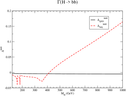
Figure 3: Pure QED (black solid) and weak (red dashed) corrections to the decay $H\rightarrow b{\overline{b}}$ as defined in Eq. 21.

The calculation of the electroweak corrections to $gb\rightarrow bH$ has many common features with that for $H\rightarrow b{\overline{b}}$ and so we review the decay process briefly. This discussion will also serve to make clear our separation of the QED and weak contributions. The electroweak corrections contain both pure QED photonic contributions and the remaining weak corrections and the two contributions are separately gauge invariantKniehl:1991ze .

The corrections to $H\rightarrow b{\overline{b}}$ can be parameterized as,

$$\Gamma(H\rightarrow b{\overline{b}})=\Gamma(H\rightarrow b{\overline{b}})_{0}\biggl{(}1+\Delta_{QCD}^{bbH}+\Delta_{QED}^{bbH}+\Delta_{WK}^{bbH}\biggr{)}\,,$$ (21)

where $\Gamma(H\rightarrow b{\overline{b}})_{0}$ is the tree level result, but evaluated with a running $b$ quark mass as described above. The QCD corrections are known to ${\cal O}(\alpha_{s}^{2})$, including all top quark mass effectsLarin:1995sq ; Chetyrkin:1995pd .

The QED corrections are found from the virtual photon diagram of Fig 2a, the real photon emission diagrams of Fig. 2b, and the counterterms derived from Fig. 2c,

$$\Delta_{QED}^{bbH}=\Delta_{Virt,QED}^{bbH}+\Delta_{CT,QED}^{bbH}+\Delta_{Real,QED}^{bbH}\,.$$ (22)

The virtual photon contribution in $N=4-2\epsilon$ dimensions is,

$$\Delta_{Virt,QED}^{bbH} = {\alpha\over\pi}Q_{b}^{2}\biggl{(}{4\pi\mu^{2}\over m_{b}^{2}}\biggr{)}^{\epsilon}\biggl{\{}{2\over\epsilon}+{1+\beta^{2}\over\beta}\biggl{[}-{1\over 2\epsilon}L-{L^{2}\over 4}+{\pi^{2}\over 3}+$$ (23)

$$Li_{2}\biggl{(}{1-\beta\over 1+\beta}\biggr{)}-L\ln\biggl{(}{1+\beta\over 2\beta}\biggr{)}\biggr{]}-\biggl{(}{1-\beta^{2}\over\beta}\biggr{)}L+3\biggr{\}}\,,$$

where $\beta=\sqrt{1-4m_{b}^{2}/M_{H}^{2}}$ and $L=\log((1-\beta)/(1+\beta))$. This is in agreement with Refs. Braaten:1980yq ; Drees:1990dq with the replacement ${4\over 3}\alpha_{s}\rightarrow Q_{b}^{2}\alpha$ and $Q_{b}=-{1\over 3}$.

To find the counterterms, we need the photonic contributions to Eqs. 17 and 18. By definition, $\delta G_{\mu}$ contains only the weak contributions. Similarly, the Higgs boson self-energy does not receive contributions from diagrams with photons in the internal loops. Thus, we have to separate the QED contributions to $\delta m_{b}$, $\delta Z_{L}$ and $\delta Z_{R}$ which come only from Fig. 2c . The results are well known,

$$\delta Z_{L,QED}=\delta Z_{R,QED} = -{\alpha\over 4\pi}Q_{b}^{2}\biggl{(}{4\pi\mu^{2}\over m_{b}^{2}}\biggr{)}^{\epsilon}\Gamma(1+\epsilon)\biggl{(}{3\over\epsilon}+4\biggr{)}$$

$$\biggl{(}{\delta m_{b}\over m_{b}}\biggr{)}_{QED} = -{\alpha\over 4\pi}Q_{b}^{2}({4\pi\mu^{2}\over m_{b}^{2}}\biggr{)}^{\epsilon}\Gamma(1+\epsilon)\biggl{(}{3\over\epsilon}+4\biggr{)}\,.$$ (24)

The QED counterterm is then,

$$\Delta_{CT,QED} = 2\biggl{\{}{\delta m_{b}\over m_{b}}+{\delta Z_{L}+\delta Z_{R}\over 2}\biggr{\}}$$ (25)

$$= -{\alpha\over\pi}Q_{b}^{2}\biggl{(}{4\pi\mu^{2}\over m_{b}^{2}}\biggr{)}^{\epsilon}\Gamma(1+\epsilon)\biggl{\{}{3\over\epsilon}+4\biggr{\}}\,.$$

Finally, we need the real photon emission contributions from Fig 2b,

$$\Delta_{Real,QED}={\alpha\over\pi}Q_{b}^{2}\biggl{(}{4\pi\mu^{2}\over m_{b}^{2}}\biggr{)}^{\epsilon}\Gamma(1+\epsilon)\biggl{\{}{1\over\epsilon}\biggl{[}1+{1+\beta^{2}\over 2\beta}L\biggr{]}+F(M_{H},\beta)\,,$$ (26)

where $F(M_{H}.\beta)$ is finite and an analytic form can be found in Refs.Drees:1990dq ; Braaten:1980yq ; Kniehl:1991ze ; Dabelstein:1991ky .

The QED contributions enumerated above are recognized by the explicit over-all factors of $Q_{b}^{2}$. The remaining weak corrections to $H\rightarrow b{\overline{b}}$, $\Delta_{WK}^{bbH}$, are given analytically in Refs. Kniehl:1991ze ; Dabelstein:1991ky and are found from diagrams with $W$’s, $Z$’s, and Goldstone bosons, along with top quark contributions. In Fig. 3 we plot the QED and weak contributions to $\Gamma(H\rightarrow b{\overline{b}})$. The QED corrections are always ${\cal O}(10^{-3})$ and can safely be neglected for all practical purposes.

II.3 One-Loop Corrections

The one loop weak corrections to the process $bg\rightarrow bH$ consist of self energy, vertex, and box diagrams (Figs. 4-6), along with the counterterms given explicitly in Eq. 17. Our results can be expressed as,

$$\sigma(bg\rightarrow bH)_{NLO}=\sigma(bg\rightarrow bH)_{0}\biggl{(}1+\Delta_{QCD}+\Delta_{QED}+\Delta_{WK}\biggr{)}\,,$$ (27)

where $\sigma_{0}$ is the Born cross section of Eq. 4 evaluated with the $1-$ loop renormalization group improved value for ${\overline{g_{b}}}$.

The purely photonic QED corrections consist of vertex and box contributions from internal photons along with the corresponding counterterms, real radiation from $bg\rightarrow bH\gamma$, and the process involving photons in the initial state, $\gamma b\rightarrow bgH$. The ${\cal O}(\alpha)$ QED corrections to $bg\rightarrow bH$ can be found from the corresponding QCD corrections by making the substitution ${4\over 3}\alpha_{s}\rightarrow\alpha Q_{b}^{2}$Dawson:2005vi ; Dawson:2003kb ; Campbell:2004pu ; Dawson:2004sh ; Dittmaier:2003ej ; Campbell:2002zm .However, evaluating the process $\gamma b\rightarrow bgH$ requires the use of a PDF set which includes initial state photons. This contribution is expected to be quite small since potentially large logarithms from initial state collinear photon emission are absorbed into the PDFs. We further note that the QED contributions to the $b{\overline{b}}\rightarrow H$ process Dittmaier:2006cz , and to the corresponding decay $H\rightarrow b{\overline{b}}$Kniehl:1991ze ; Dabelstein:1991ky discussed above, are known to be less than $1~{}\%$. As this is considerably smaller than the PDF and scale uncertainties which we present in the next section, we do not provide numerical results for the pure QED corrections to $bg\rightarrow bH$, but evaluate only the weak corrections.

The Feynman diagrams are generated using FeynArtsHahn:2000kx and the interference with the tree level amplitude is evaluated numerically in Feynman gauge using FormCalc and LoopToolsHahn:1998yk . We retain a non-zero bottom quark mass everywhere.

Figure 4: Self energy diagrams contributing to the weak corrections to $bg\rightarrow bH$.

Figure 5: Vertex diagrams contributing to the weak corrections to $bg\rightarrow bH$.

Figure 6: Box diagrams contributing to the weak corrections to $bg\rightarrow bH$.

II.4 Large Higgs Mass Limit

The contributions to the weak corrections in the large Higgs mass limit can be easily found and provide a check of our results. The large Higgs mass limit for the process $bg\rightarrow bH$ is obtained by noting that the triangle and box diagrams shown in Figs. 4 -6 are of ${\cal O}\biggl{(}{m_{b}^{2}\over v^{2}}\biggr{)}$ relative to the tree level amplitude. The only contributions which are enhanced by factors of ${M_{H}^{2}\over v^{2}}$ come from the renormalization of the $b\overline{b}H$ vertex, Eq. 1. In the large $M_{H}$ limit,

$$L_{YUK}\rightarrow{m_{b}e\over 2M_{W}}\biggl{(}{Z_{H}\over 1+\delta M_{W}^{2}/M_{W}^{2}}\biggr{)}{\overline{b}}bH+{\rm terms~{}not~{}enhanced~{}by~{}}{M_{H}^{2}\over v^{2}}\,.$$ (28)

The large $M_{H}$ limit of the Higgs wavefunction renormalization isMarciano:1987un ; Dawson:1989up ,

$$Z_{H}=1+{1\over 16\pi^{2}}{M_{H}^{2}\over v^{2}}\biggl{(}6-\pi\sqrt{3}\biggr{)}\,.$$ (29)

Similarly, the $W$ mass renormalization receives a contribution proportional to $M_{H}^{2}$,

$${\delta M_{W}^{2}\over M_{W}^{2}}=-{1\over 32\pi^{2}}{M_{H}^{2}\over v^{2}}\,.$$ (30)

The leading $M_{H}$ corrections to $bH$ production are thereforeMarciano:1987un ,

$$\sigma(bg\rightarrow bH) \rightarrow {Z_{H}\over 1+{\delta M_{W}^{2}\over M_{W}^{2}}}\sigma(bg\rightarrow bH)_{0}$$ (31)

$$= \biggl{(}1+{1\over 32\pi^{2}}{M_{H}^{2}\over v^{2}}\biggl{[}13-{2\pi\sqrt{3}}\biggr{]}\biggr{)}\sigma(bg\rightarrow bH)_{0}$$

$$\equiv \biggl{(}1+\Delta_{EW}^{M_{H}\rightarrow\infty}\biggr{)}\sigma(bg\rightarrow bH)_{0}\,.$$

III Results

III.1 Numerical Results

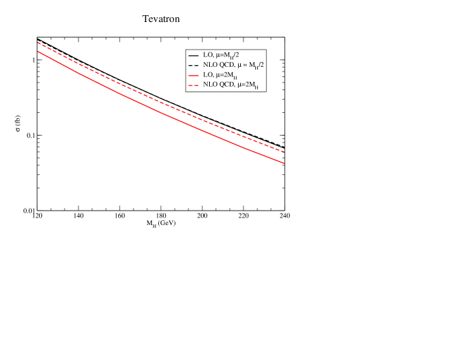
Figure 7: Lowest order and NLO QCD results for $p{\overline{p}}\rightarrow b({\overline{b}})HX$ at the Tevatron with $\sqrt{s}=1.96~{}TeV$ with $\sqrt{s}=1.96~{}GeV$, $p_{T}^{b}>20~{}GeV$, $\mid\eta_{b}\mid<2$, and $\Delta R>.4$. The renormalization/factorization scales are set equal to $\mu$.

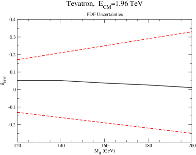
Figure 8: PDF uncertainties for $p{\overline{p}}\rightarrow b({\overline{b}})HX$ at the Tevatron with $\sqrt{s}=1.96~{}TeV$ $p_{T}^{b}>20~{}GeV$, $\mid\eta_{b}\mid<2$, $\Delta R>.4$, and $\mu=M_{H}/2$. The solid line is $\sigma_{NLO}(CTEQ6.6)/\sigma_{NLO}(MRSW)-1$. The dashed curves are the percentage variations from the central prediction between the upper and lower predictions obtained using the CTEQ6.6 PDF error sets.

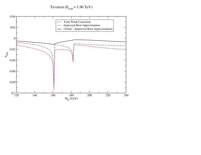
Figure 9: Tevatron results for the weak corrections to $p{\overline{p}}\rightarrow b({\overline{b}})H$ with $\sqrt{s}=1.96~{}GeV$, $p_{T}^{b}>20~{}GeV$, and $\mid\eta_{b}\mid<2$. The solid black curve represents the contributions which cannot be factorized into an effective ${\overline{b}}bH$ vertex contribution and is always less than $1\%$.

For our numerical studies, we use the following inputs:

$$\alpha = 1/137.03599911$$

$$G_{\mu} = 1.16637\times 10^{-5}~{}GeV^{-2}$$

$$M_{Z} = 91.1875~{}GeV$$

$$M_{t} = 173.1~{}GeV\,.$$ (32)

We set the CKM mixing matrix to unity. For the pole mass of the $b$ quark, we take $M_{b}=4.25~{}GeV$. We use CTEQ6.6 PDFsNadolsky:2008zw and vary the renormalization/factorization scales $\mu=\mu_{R}=\mu_{F}$ from $M_{H}/2$ to $2M_{H}$ in the total cross section results.

Our results are expressed as,

$$\sigma(bg\rightarrow bH)_{NLO}(\mu)=\sigma(bg\rightarrow bH)_{0}(\mu)\biggl{(}1+\Delta_{QCD}(\mu)+\Delta_{QED}(\mu)+\Delta_{WK}(\mu)\biggr{)}\,,$$ (33)

where $\sigma_{0}$ is the Born cross section of Eq. 4 evaluated with the $1-$ loop renormalization group improved value for ${\overline{g_{b}}}(\mu)$ and includes the full $m_{b}$ mass dependence of Eq. 4. (Including the $m_{b}$ dependence has almost no numerical effect).

The NLO QCD corrections are parameterized by the factor $\Delta_{QCD}$ and $\sigma_{NLO}$ is evaluated with the $2-$ loop renormalization group improved value for ${\overline{g_{b}}}(\mu)$. The NLO QCD corrections to the $bg\rightarrow bH$ process have been previously found in the S-ACOT scheme, which includes all effects of the finite $b$ mass to ${\cal O}(\alpha_{s})$. In the S-ACOT schemeKramer:2000hn , effects of a non-zero $b$ quark mass in the process $bg\rightarrow bH$ are absorbed into the definition of the PDFs and to ${\cal O}(\alpha_{s})$, we have schematically,

$$\sigma_{NLO,QCD}(pp\rightarrow bH)_{m_{b}\neq 0} \equiv \sigma_{LO}(pp\rightarrow bH)_{m_{b}=0}(1+\delta_{QCD})+{\cal O}(\alpha_{s}^{2})$$

$$\Delta_{QCD} = {\sigma_{LO}(pp\rightarrow bH)_{m_{b}=0}\over\sigma_{LO}(pp\rightarrow bH)_{m_{b}\neq 0}}\delta_{QCD}\,,$$ (34)

where $\delta_{QCD}$ is given in Ref. Campbell:2002zm . Both the CTEQ and MRSW PDF sets employ the S-ACOT scheme and so our inclusion of $b$ mass effects is consistent to ${\cal O}(\alpha_{s})$.

The QED and weak corrections are contained in $\Delta_{QED}$ and $\Delta_{WK}$, respectively. As discussed above, we do not present results for $\Delta_{QED}$, but assume they are negligible. The contribution of $\Delta_{WK}$ results from the interference of the tree level amplitude with the $1$-loop amplitudes shown above, which are generated numerically. We compare our exact results of Eq. 33 with an “Improved Born Approximation”, IBA, which is obtained by replacing the tree level ${\overline{b}}bH$ vertex of Eq. 1 with the on-shell one loop electroweak corrected vertex which can be found from the corrections to the decay $H\rightarrow b{\overline{b}}$Kniehl:1991ze ; Dabelstein:1991ky ,

$$\Gamma(H\rightarrow b{\overline{b}})=\Gamma(H\rightarrow b{\overline{b}})_{0}\biggl{(}1+\Delta_{QCD}^{bbH}+\Delta_{QED}^{bbH}+\Delta_{WK}^{bbH}\biggr{)}\,.$$ (35)

We define the Improved Born Approximation in an obvious fashion as

$$\sigma(bg\rightarrow bH)_{IBA}(\mu)\equiv\sigma(bg\rightarrow bH)_{0}(\mu)\biggl{(}1+\Delta_{QCD}^{bbH}+\Delta_{EM}^{bbH}+\Delta_{WK}^{bbH}\biggr{)}\,.$$ (36)

The IBA approximation assumes that the bulk of the weak corrections modify the ${\overline{b}}bH$ vertex. In the case of the SUSY QCD corrections to $bg\rightarrow bH$ from squarks and gluinos, the Improved Born Approximation is an excellent approximation to the full rateDawson:2007ur .

Results for the Tevatron are shown in Figs. 7, 8, and 9. The Tevatron plots have $\sqrt{s}=1.96~{}TeV$, $\mid\eta_{b}\mid<2.0$ and require $p_{T}^{b}>20~{}GeV$. The NLO QCD corrections combine partons if $\Delta R\equiv\sqrt{(\Delta\phi)^{2}+(\Delta\eta)^{2}}<0.4$. For $M_{H}=160$ GeV, the scale uncertainty at NLO with a variation from $\mu=M_{H}/2$ to $2M_{H}$ is $\sim 10\%$, while for $M_{H}=120~{}GeV$ it is $\sim 8\%$. The PDF uncertainties are estimated in Fig. 8 where we compare the CTEQ6.6 predictions with those obtained using the MRSW2008 NLO PDFsMartin:2009iq , (with $\mu=M_{H}/2$), and find agreement between the $2$ PDF sets to within better than $5\%$. The PDF uncertainties using the CTEQ6 error sets are also shown in Fig. 8 and are quite large, varying between $15\%$ and $20\%$ for the masses considered here.

Fig. 9 shows the size of the weak corrections as defined by Eq. 33. We note that the $\mu$ dependence of $\Delta_{WK}$ is extremely small. The weak corrections are well approximated by the IBA of Eq. 36 (the dot- dashed line of Fig. 9), with the remaining corrections (the solid line in Fig. 9 ) always less than $1\%$. Except near the $W^{+}W$ and $ZZ$ resonances, $\Delta_{WK}$ in the Standard Model is significantly smaller than the uncertainties from the QCD scale variation and the PDF uncertainties.

At the LHC, we consider $\sqrt{s}=7~{}TeV$ and $\sqrt{s}=10~{}TeV$, with $\mid\eta_{b}\mid<2.5$, $p_{T}^{b}>25~{}GeV$ and $\Delta R>0.4$. The NLO QCD corrected cross sections are shown in Figs. 10 and 13. The NLO cross section is reduced by a factor of $\sim 2.2$ for $M_{H}=150~{}GeV$ (with $\mu=M_{H}/2$) when going from $\sqrt{s}=10~{}TeV$ to $7~{}TeV$. At $\sqrt{s}=7~{}TeV$, and $M_{H}=150$ GeV, the scale uncertainty at NLO with a variation from $\mu=M_{H}/2$ to $2M_{H}$ is $\sim 5\%$, while for $M_{H}=300~{}GeV$ it is $\sim 9\%$. The PDF uncertainties for $\sqrt{s}=10~{}TeV$ are estimated in Fig. 14 where we compare the CTEQ6.6 predictions with those obtained using the MRSW2008 NLO PDFsMartin:2009iq , (with $\mu=M_{H}/2$), and find agreement between the $2$ PDF sets to within better than $3\%$. The PDF uncertainties using the CTEQ6 error sets are also shown in Fig. 14 and are smaller than at the Tevatron, varying between $4\%$ and $6\%$ for the masses considered here. The PDF uncertainties are similar for $\sqrt{s}=7~{}TeV$.

The weak corrections are shown in Figs. 11 and 15 for $M_{H}<500~{}GeV$. The IBA (Eq. 36) encapsulates the total weak corrections to better than $1\%$ for $M_{H}<500~{}GeV$. We show the weak effects for $M_{H}>500~{}GeV$, along with the large $M_{H}$ limit of Eq. 31, in Figs. 12 and 16. For $M_{H}=1~{}TeV$, the IBA underestimates the total weak corrections by about $3\%$ at $\sqrt{s}=10~{}TeV$. For large $M_{H}$ ($M_{H}>2M_{t}$), the weak corrections are significant and are greater than $18\%$ for $M_{H}\sim 1~{}TeV$. We note that the large $M_{H}$ limit underestimates the weak corrections by about $5\%$ at $M_{H}=1~{}TeV$, implying that the $\log(M_{H})$ terms are numerically important. For heavy Higgs bosons, $M_{H}>500~{}GeV$, the weak corrections are larger than uncertainties from PDFs and the scale choice, and it is meanful to include them in precision calculations.

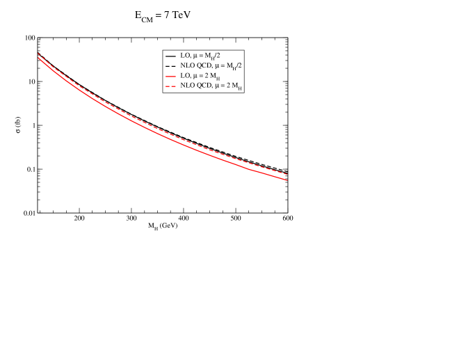
Figure 10: Lowest order and NLO QCD results for $pp\rightarrow b({\overline{b}})HX$ at the LHC with $\sqrt{s}=7~{}TeV$, $p_{T}^{b}>25~{}GeV$, $\mid\eta_{b}\mid<2.5$, and $\Delta r>.4$. The renormalization/factorization scales are set equal to $\mu$.

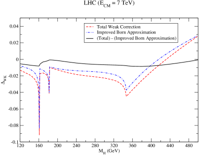
Figure 11: LHC results for the weak corrections to $pp\rightarrow b({\overline{b}})H$ with $\sqrt{s}=7~{}TeV$, $p_{T}^{b}>25~{}GeV$, and $\mid\eta_{b}\mid<2.5$. The solid black curve represents the contributions which cannot be factorized into an effective ${\overline{b}}bH$ vertex contribution and is less than $1\%$ for $M_{H}<500~{}GeV$.

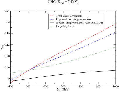
Figure 12: LHC results for the weak corrections to $pp\rightarrow b({\overline{b}})H$ with $\sqrt{s}=7~{}TeV$, $p_{T}^{b}>25~{}GeV$, and $\mid\eta_{b}\mid<2.5$. The solid black curve represents the contributions which cannot be factorized into an effective ${\overline{b}}bH$ vertex contribution. The dotted line is the large Higgs mass limit of Eq. 31.

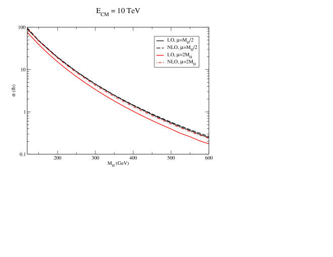
Figure 13: Lowest order and NLO QCD results for $pp\rightarrow b({\overline{b}})HX$ at the LHC with $\sqrt{s}=10~{}TeV$, $p_{T}^{b}>25~{}GeV$, $\mid\eta_{b}\mid<2.5$, and $\Delta r>.4$. The renormalization/factorization scales are set equal to $\mu$.

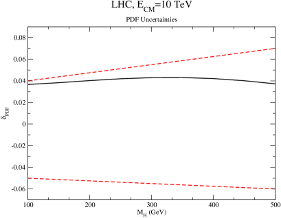
Figure 14: PDF uncertainties for $pp\rightarrow b({\overline{b}})H$ at the LHC with $\sqrt{s}=10~{}TeV$, $p_{T}^{b}>25~{}GeV$, $\mid\eta_{b}\mid<2.5$, $\Delta R>.4$, and $\mu=M_{H}/2$. The solid line is $\sigma_{NLO}(CTEQ6.6)/\sigma_{NLO}(MRSW)-1$. The dashed curves are the percentage variations from the central prediction between the upper and lower predictions obtained using the CTEQ6.6 PDF error sets.

Figure 15: LHC results for the weak corrections to $pp\rightarrow b({\overline{b}})H$ with $\sqrt{s}=10~{}TeV$, $p_{T}^{b}>25~{}GeV$, and $\mid\eta_{b}\mid<2.5$. The solid black curve represents the contributions which cannot be factorized into an effective ${\overline{b}}bH$ vertex contribution and is less than $1\%$ for $M_{H}<500~{}GeV$.

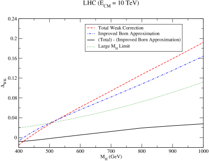
Figure 16: LHC results for the weak corrections to $pp\rightarrow b({\overline{b}})H$ with $\sqrt{s}=10~{}TeV$, $p_{T}^{b}>25~{}GeV$, and $\mid\eta_{b}\mid<2.5$. The solid black curve represents the contributions which cannot be factorized into an effective ${\overline{b}}bH$ vertex contribution. The dotted line is the large Higgs mass limit of Eq. 31.

III.2 The $m_{b}=0$ Limit

It is interesting to consider the $m_{b}\rightarrow 0$ limit of the $bg\rightarrow bH$ amplitude. In this limit, the $b$-Higgs Yukawa coupling vanishes, $g_{b}=m_{b}/v\rightarrow 0$, and the tree level amplitude shown in Fig. 1 is identically zero. The first non-zero contributions to $bg\rightarrow bH$ with $m_{b}=0$ arise from the squares of a subset of the $1-$ loop amplitudes shown in Figs. 5 and 6 and are ${\cal O}(\alpha_{s}G_{F}^{3})$. The contributions which are non-zero in the $m_{b}\rightarrow 0$ limit involve the coupling of the Higgs to either a top quark or a pair of gauge bosons (and the corresponding Goldstone bosons). These contributions have been calculated in Ref. Mrenna:1995cf and we have checked that the squares of our $1-$ loop amplitudes reproduce their results in the $m_{b}=0$ limit. Since these diagrams are not suppressed by a small $b$ quark Yukawa coupling, they give a comparatively large contribution. At $\sqrt{s}=7~{}TeV$ and $M_{H}=120~{}GeV$, we find that the ${\cal O}(\alpha_{s}G_{F}^{3})$ contribution with $m_{b}=0$ is around $8\%$ of the Born cross section shown in Fig.10 with our cuts.

Although our calculations are purely Standard Model, we are, however, motivated by a very different scenario than the authors of Ref. Mrenna:1995cf . In models with an enhanced coupling of the $b$ quark to a Higgs boson, the tree level amplitude can be significantly larger than in the Standard Model. In such models, it is important to understand the numerical effect of the interference of the tree level amplitude with the one-loop weak corrections. Future work will explore the role of the electroweak corrections in models with non-standard $b$ quark Higgs Yukawa couplings, in particular the MSSM with large $\tan\beta$.

IV Conclusion

We have computed the Standard Model weak corrections to the processes $pp\rightarrow b({\overline{b}})H$ at the LHC and $p{\overline{p}}\rightarrow b({\overline{b}})H$ at the Tevatron. In both cases, the results are well approximated by including only the on-shell ${\overline{b}}bH$ vertex corrections, with the remaining weak corrections less than $1-2\%$ for $M_{H}<500~{}GeV$. This observation makes it straightforward to estimate the weak effects of non-Standard Model $b$ quark Yukawa couplings on the $bH$ production process.

At the Tevatron, the weak effects are always much smaller than scale and PDF uncertainties and so can be neglected in the Standard Model. At the LHC, for large $M_{H}$ the weak corrections can become significant and can be larger than scale and PDF uncertainties. At the LHC with $\sqrt{s}=10~{}TeV$, the corrections of ${\cal O}\biggl{(}{M_{H}^{2}\over v^{2}}\biggr{)}$ are $\sim 18\%$ for $M_{H}=1~{}TeV$.

References

• (1) S. Dawson, C. B. Jackson, L. Reina, and D. Wackeroth. Higgs production in association with bottom quarks at hadron colliders. Mod. Phys. Lett., A21:89–110, 2006.
• (2) S. Dawson, C. B. Jackson, L. Reina, and D. Wackeroth. Higgs boson production with one bottom quark jet at hadron colliders. Phys. Rev. Lett., 94:031802, 2005.
• (3) J. Campbell et al. Higgs boson production in association with bottom quarks. 2004.
• (4) Stefan Dittmaier, Michael Kramer, and Michael Spira. Higgs radiation off bottom quarks at the tevatron and the lhc. Phys. Rev., D70:074010, 2004.
• (5) S. Dawson, C. B. Jackson, L. Reina, and D. Wackeroth. Exclusive higgs boson production with bottom quarks at hadron colliders. Phys. Rev., D69:074027, 2004.
• (6) John M. Campbell, R. Keith Ellis, F. Maltoni, and S. Willenbrock. Higgs boson production in association with a single bottom quark. Phys. Rev., D67:095002, 2003.
• (7) Fabio Maltoni, Thomas McElmurry, and Scott Willenbrock. Inclusive production of a higgs or z boson in association with heavy quarks. Phys. Rev., D72:074024, 2005.
• (8) D. Dicus, T. Stelzer, Z. Sullivan, and S. Willenbrock. Higgs boson production in association with bottom quarks at next-to-leading order. Phys. Rev., D59:094016, 1999.
• (9) F. Maltoni, Z. Sullivan, and S. Willenbrock. Higgs-boson production via bottom-quark fusion. Phys. Rev., D67:093005, 2003.
• (10) Oliver Brein and Wolfgang Hollik. Mssm higgs bosons associated with high-p(t) jets at hadron colliders. Phys. Rev., D68:095006, 2003.
• (11) B. Field, S. Dawson, and J. Smith. Scalar and pseudoscalar Higgs boson plus one jet production at the LHC and Tevatron. Phys. Rev., D69:074013, 2004.
• (12) Marcela S. Carena, S. Mrenna, and C. E. M. Wagner. Mssm higgs boson phenomenology at the tevatron collider. Phys. Rev., D60:075010, 1999.
• (13) Marcela S. Carena, A. Menon, and C. E. M. Wagner. Challenges for mssm higgs searches at hadron colliders. Phys. Rev., D76:035004, 2007.
• (14) R. Michael Barnett, Howard E. Haber, and Davison E. Soper. Ultraheavy particle production from heavy partons at hadron colliders. Nucl. Phys., B306:697, 1988.
• (15) Fredrick I. Olness and Wu-Ki Tung. When is a heavy quark not a parton? charged higgs production and heavy quark mass effects in the qcd based parton model. Nucl. Phys., B308:813, 1988.
• (16) Robert V. Harlander and William B. Kilgore. Higgs boson production in bottom quark fusion at next-to- next-to-leading order. Phys. Rev., D68:013001, 2003.
• (17) Stefan Dittmaier, Michael Kramer, 1, Alexander Muck, and Tobias Schluter. MSSM Higgs-boson production in bottom-quark fusion: Electroweak radiative corrections. JHEP, 03:114, 2007.
• (18) Wolfgang Hollik and Michael Rauch. Higgs-Boson Production in Association with Heavy Quarks. AIP Conf. Proc., 903:117–120, 2007.
• (19) S. Dawson and C. B. Jackson. SUSY QCD Corrections to Associated Higgs-bottom Quark Production. Phys. Rev., D77:015019, 2008.
• (20) V. M. Abazov et al. Search for neutral Higgs bosons in multi-b-jet events in $p\bar{p}$ collisions at $\sqrt{s}$ = 1.96-TeV. Phys. Rev. Lett., 101:221802, 2008.
• (21) V. M. Abazov et al. Search for neutral Higgs bosons $tan\beta$ in the b(h/H/A) $\to b\tau\tau$ channel . Phys. Rev. Lett., 102:051804, 2009.
• (22) Fawzi Boudjema and Le Duc Ninh. b anti-b Higgs production at the LHC: Yukawa corrections and the leading Landau singularity. Phys. Rev., D78:093005, 2008.
• (23) S. Mrenna and C. P. Yuan. High $p_{T}$ Higgs boson production at hadron colliders to O (alpha-s G(F) (3) ). Phys. Rev., D53:3547–3554, 1996.
• (24) Bernd A. Kniehl and Michael Spira. Two loop O (alpha-s G(F) $m($t$)^{2}$ correction to the $H\to b\bar{b}$ decay rate. Nucl. Phys., B432:39–48, 1994.
• (25) Abdelhak Djouadi. The Anatomy of electro-weak symmetry breaking. I: The Higgs boson in the standard model. Phys. Rept., 457:1–216, 2008.
• (26) W. F. L. Hollik. Radiative Corrections in the Standard Model and their Role for Precision Tests of the Electroweak Theory. Fortschr. Phys., 38:165–260, 1990.
• (27) Dmitri Yu. Bardin and G. Passarino. The standard model in the making: Precision study of the electroweak interactions. Oxford, UK: Clarendon (1999) 685 p.
• (28) Mu-Chun Chen, Sally Dawson, and C. B. Jackson. Higgs Triplets, Decoupling, and Precision Measurements. Phys. Rev., D78:093001, 2008.
• (29) Mu-Chun Chen and Sally Dawson. One-loop radiative corrections to the rho parameter in the littlest Higgs model. Phys. Rev., D70:015003, 2004.
• (30) H. Burkhardt and B. Pietrzyk. Update of the hadronic contribution to the QED vacuum polarization. Phys. Lett., B513:46–52, 2001.
• (31) A. Sirlin and W. J. Marciano. Radiative Corrections to Muon-neutrino N $\to$ mu- X and their Effect on the Determination of rho**2 and sin**2- Theta(W). Nucl. Phys., B189:442, 1981.
• (32) A. Sirlin. Radiative Corrections in the SU(2)-L x U(1) Theory: A Simple Renormalization Framework. Phys. Rev., D22:971–981, 1980.
• (33) William J. Marciano and A. Sirlin. Testing the Standard Model by Precise Determinations of W+- and Z Masses. Phys. Rev., D29:945, 1984.
• (34) Bernd A. Kniehl. Radiative corrections for $H\to$ f anti-f ($\gamma$) in the standard model. Nucl. Phys., B376:3–28, 1992.
• (35) S. A. Larin, T. van Ritbergen, and J. A. M. Vermaseren. The Large top quark mass expansion for Higgs boson decays into bottom quarks and into gluons. Phys. Lett., B362:134–140, 1995.
• (36) K. G. Chetyrkin and A. Kwiatkowski. Second order QCD corrections to scalar and pseudoscalar Higgs decays into massive bottom quarks. Nucl. Phys., B461:3–18, 1996.
• (37) Manuel Drees and Ken-ichi Hikasa. NOTE ON QCD CORRECTIONS TO HADRONIC HIGGS DECAY. Phys. Lett., B240:455, 1990.
• (38) E. Braaten and J. P. Leveille. Higgs Boson Decay and the Running Mass. Phys. Rev., D22:715, 1980.
• (39) A. Dabelstein and W. Hollik. Electroweak corrections to the fermionic decay width of the standard Higgs boson. Z. Phys., C53:507–516, 1992.
• (40) Ansgar Denner, S. Dittmaier, M. Roth, and L. H. Wieders. Electroweak corrections to charged-current e+ e- –¿ 4 fermion processes: Technical details and further results. Nucl. Phys., B724:247–294, 2005.
• (41) Giampiero Passarino, Christian Sturm, and Sandro Uccirati. Higgs Pseudo-Observables, Second Riemann Sheet and All That. 2010.
• (42) A. D. Martin, R. G. Roberts, W. J. Stirling, and R. S. Thorne. Parton distributions incorporating QED contributions. Eur. Phys. J., C39:155–161, 2005.
• (43) Thomas Hahn. Generating Feynman diagrams and amplitudes with FeynArts 3. Comput. Phys. Commun., 140:418–431, 2001.
• (44) T. Hahn and M. Perez-Victoria. Automatized one-loop calculations in four and D dimensions. Comput. Phys. Commun., 118:153–165, 1999.
• (45) William J. Marciano and Scott S. D. Willenbrock. RADIATIVE CORRECTIONS TO HEAVY HIGGS SCALAR PRODUCTION AND DECAY. Phys. Rev., D37:2509, 1988.
• (46) Sally Dawson and Scott Willenbrock. RADIATIVE CORRECTIONS TO LONGITUDINAL VECTOR BOSON SCATTERING. Phys. Rev., D40:2880, 1989.
• (47) Pavel M. Nadolsky et al. Implications of CTEQ global analysis for collider observables. Phys. Rev., D78:013004, 2008.
• (48) http://mcfm.fnal.gov.
• (49) Michael Kramer, 1, Fredrick I. Olness, and Davison E. Soper. Treatment of heavy quarks in deeply inelastic scattering. Phys. Rev., D62:096007, 2000.
• (50) A. D. Martin, W. J. Stirling, R. S. Thorne, and G. Watt. Parton distributions for the LHC. Eur. Phys. J., C63:189–285, 2009.