Derivation of Stochastic Acceleration Model Characteristics for Solar Flares From RHESSI Hard X-Ray Observations

Abstract

The model of stochastic acceleration of particles by turbulence has been successful in explaining many observed features of solar flares. Here we demonstrate a new method to obtain the accelerated electron spectrum and important acceleration model parameters from the high resolution hard X-ray observations provided by the Reuven Ramaty High Energy Solar Spectroscopic Imager (RHESSI). In our model, electrons accelerated at or very near the loop top produce thin target bremsstrahlung emission there and then escape downward producing thick target emission at the loop footpoints. Based on the electron flux spectral images obtained by the regularized inversion of the RHESSI count visibilities, we derive several important parameters for the acceleration model. We apply this procedure to the 2003 November 03 solar flare, which shows a loop top source up to 100–150 keV in hard X-ray with a relatively flat spectrum in addition to two footpoint sources. The results imply presence of strong scattering and a high density of turbulence energy with a steep spectrum in the acceleration region.

1. Introduction

It is well established that the impulsive phase hard X-ray (HXR) emission of solar flares is produced by bremsstrahlung of nonthermal electrons spiraling down the flare loop while losing energy primarily via elastic Coulomb collisions (Brown, 1971; Hudson, 1972; Petrosian, 1973). Thus, HXR observations provide the most direct information on the spectrum of the radiating electrons and perhaps on the mechanism responsible for their acceleration. The common practice to extract this information has been to use the parametric forward fitting of HXR spectra to emission by an assumed spectrum, usually a power-law with breaks and cutoffs (or plus a thermal component), of the radiating or accelerated electrons (e.g. Holman et al., 2003). A more direct connection was established between the observations and the acceleration process first by Hamilton & Petrosian (1992), fitting to high spectral resolution but narrow band observations (Lin & Schwartz, 1987), and later by Park et al. (1997), fitting to broad band observations (e.g. Marschhäuser et al., 1994; Dingus et al., 1994). This was done in the framework of stochastic acceleration (SA) by plasma waves or turbulence.

However, it is preferable to obtain the X-ray radiating electron spectrum nonparametrically by some inversion techniques first attempted by Johns & Lin (1992). Recently, Piana et al. (2003) and Kontar et al. (2004) applied regularized inversion techniques to obtain the radiating electron flux spectra from the spatially integrated photon spectra observed by RHESSI (Lin et al., 2002). This is an important advance but it gives the spectrum of the effective radiating electrons summed over the whole flare loop, but not the spectrum of the accelerated electrons. This difference arises because high spatial resolution observations, first from Yohkoh (Masuda et al., 1994; Petrosian et al., 2002) and now from RHESSI (e.g. Liu et al., 2003), have shown that, essentially for all flares, in addition to the emission from the loop footpoints (FPs) (e.g. Hoyng et al., 1981), there is substantial HXR emission from a region near the loop top (LT). Thus, the total radiating electron spectrum is a complex combination of the accelerated electrons at the LT and those present in the FPs after having been modified by transport effects.

It is therefore clear that separate inversion of the LT and FP photon spectra to electron spectra would provide more direct information on the acceleration mechanism. More recently, Piana et al. (2007) have applied the regularized inversion technique to the RHESSI data in the Fourier domain (Hurford et al., 2002) to obtain electron flux spectral images. The goal of this letter is to demonstrate that with the resulting spatially resolved electron flux spectra at the LT and FPs one can begin to constrain the acceleration model parameters directly.

In the next section we present a brief review of the relation between the derived electron flux images and the characteristics of the SA model and in §3 we apply this relation to a flare observed by RHESSI. A brief summary and our conclusion are presented in §4.

2. Acceleration and Radiation

The observations of distinct LT and FP HXR emissions, with little or no emission from the legs of the loop, point to the LT as the acceleration site and require enhanced scattering of electrons in the LT. Petrosian & Donaghy (1999) showed that the most likely scattering agent is turbulence which can also accelerate particles stochastically. In fact SA of the background thermal plasma has been the leading mechanism for acceleration of electrons (e.g. Hamilton & Petrosian, 1992; Miller et al., 1996; Park et al., 1997; Petrosian & Liu, 2004; Grigis & Benz, 2006; Bykov & Fleishman, 2009) and ions (e.g. Ramaty, 1979; Mason et al., 1986; Mazur et al., 1995; Liu et al., 2004, 2006; Petrosian et al., 2009), and is the most developed model in terms of comparing with observations.

2.1. Particle Kinetic Equation

In this model one assumes that turbulence is produced at or near the LT region (with background electron density $n_{\rm LT}$, volume $V$, and size $L$). In presence of a sufficiently high density of turbulence the scattering can result in a mean scattering length or time ($\tau_{\rm scat}$) smaller than $L$ or the crossing time ($\tau_{\rm cross}=L/v$), leading to a nearly isotropic pitch angle distribution (Petrosian & Liu, 2004). The general Fokker-Planck equation for the density spectrum $N(E)$ of the accelerated electrons, averaged over the turbulent acceleration region, simplifies to

$$\frac{\partial N}{\partial t}=\frac{\partial^{2}}{\partial E^{2}}\left[D_{\rm EE}N\right] - \frac{\partial}{\partial E}\left[\left(A(E)-\dot{E}_{\rm L}(E)\right)N\right]$$ (1)

$$- \frac{N}{T_{\rm esc}(E)}+\dot{Q}(E),$$

where $D_{\rm EE}(E)$ and $A(E)$ are the diffusion rate and direct acceleration rate by turbulence, respectively, $\dot{E}_{\rm L}$ is the electron energy loss rate, and $\dot{Q}(E)$ and $N(E)/T_{\rm esc}(E)$ describe the rate of injection of (thermal) particles and escape of the accelerated particles from the acceleration region. For electrons of energies below $\sim$1 MeV, which are of interest here, Coulomb collisions dominate the energy loss rate,

$$\dot{E}_{\rm L}=\dot{E}_{\rm Coul}=4\pi r_{0}^{2}m_{\rm e}c^{3}n_{\rm LT}\ln\Lambda/\beta,$$ (2)

where $\ln\Lambda$ is the Coulomb logarithm taken to be 20 for solar flare conditions. Following Petrosian & Liu (2004), we approximate the escape time as $T_{\rm esc}(E)\simeq\tau_{\rm cross}(1+\tau_{\rm cross}/\tau_{\rm scat})$, which smoothly connects the two limiting cases of $\tau_{\rm cross}/\tau_{\rm scat}\gg 1$ and $\ll 1$. The mean scattering time is related to the pitch angle diffusion rates (Dung & Petrosian, 1994; Pryadko & Petrosian, 1997) due to both Coulomb collisions ($D^{\rm Coul}_{\rm\mu\mu}$ and $\tau^{\rm turb}_{\rm scat}$) and turbulence ($D^{\rm turb}_{\rm\mu\mu}$ and $\tau^{\rm Coul}_{\rm scat}$) as

$$\tau_{\rm scat}(E)=\frac{1}{8}\int_{-1}^{1}\frac{(1-\mu^{2})^{2}}{D_{\mu\mu}^{\rm Coul}(\mu,E)+D_{\mu\mu}^{\rm turb}(\mu,E)}{\rm d}\mu.$$ (3)

Similarly we can define the scattering times $\tau^{\rm Coul}_{\rm scat}$ and $\tau^{\rm turb}_{\rm scat}$ for each process alone. For Coulomb collisions, $D_{\mu\mu}^{\rm Coul}=\frac{2(1-\mu^{2})}{\gamma+1}\frac{\dot{E}_{\rm Coul}}{{E}}$. For turbulence, $D^{\rm turb}_{\mu\mu}$, like $D_{\rm EE}$, depends on the spectrum of turbulence and on the background plasma density, composition, temperature, and magnetic field (see Schlickeiser, 1989; Dung & Petrosian, 1994; Pryadko & Petrosian, 1997, 1998, 1999; Petrosian & Liu, 2004). Since these coefficients determine the spectrum of the accelerated electrons, one can then constrain some aspects of the acceleration mechanism if an accurate spectrum of the electrons can be derived from observations.

2.2. LT and FP Spectra

The accelerated electrons in the (LT) acceleration region with a flux spectrum $F_{\rm LT}(E)=vN(E)$ produce thin target bremsstrahlung emissivity (photons s^-1 keV^-1)

$$J_{\rm LT}(\epsilon)=n_{\rm LT}V\int_{\epsilon}^{\infty}F_{\rm LT}(E)\sigma(\epsilon,E){\rm d}E,$$ (4)

where $\sigma(\epsilon,E)$ is the angle-averaged bremsstrahlung cross section (Koch & Motz, 1959). The escaping electrons with flux $F_{\rm 0}(E)=N(E)L/T_{\rm esc}$ produce thick target bremsstrahlung emissivity (coming mostly from the FPs) (see Petrosian, 1973; Park et al., 1997),

$$J_{\rm FP}(\epsilon)=nV\int_{\epsilon}^{\infty}F_{\rm FP}(E)\sigma(\epsilon,E){\rm d}E,$$ (5)

where $n$ is the density and $F_{\rm FP}$ is the effective radiating electron flux spectrum at the FPs,

$$F_{\rm FP}(E)=vN_{\rm FP}=\frac{v(E)}{\dot{E}_{\rm L}(n)}\int_{E}^{\infty}\frac{N(E^{\prime})}{T_{\rm esc}(E^{\prime})}{\rm d}E^{\prime}.$$ (6)

Since $\dot{E}_{\rm L}\propto n$, the FP photon spectrum is independent of density. In what follows we evaluate equations (5) and (6) using the LT density $n_{\rm LT}$.

2.3. Acceleration Model Parameters

Regularized inversion of RHESSI count visibilities gives the electron visibilities (Piana et al., 2007), which can then be used to construct images of electron flux (multiplied by column density). From these images, we extract the spatially resolved spectra, $F_{\rm LT}(E)$ at the LT and $F_{\rm FP}(E)$ at the FPs. Thus we can obtain the accelerated electron spectrum $N(E)$ at the thin target LT. Also from differentiation of equation (6) we derive the escape time as $T_{\rm esc}=-N(E)/\frac{\rm d}{{\rm d}E}(F_{\rm FP}\dot{E}_{\rm L}/v)$, and by converting the denominator to a logarithm derivative we get

$$T_{\rm esc}(E)=\frac{\tau_{\rm L}(E)(F_{\rm LT}/F_{\rm FP})}{\delta_{\rm FP}(E)+2/(\gamma+\gamma^{2})}\equiv\tau_{\rm L}(E)\xi(E),$$ (7)

where the FP index $\delta_{\rm FP}(E)=-\frac{{\rm d}\ln F_{\rm FP}}{{\rm d}\ln E}$, $1/(\gamma+\gamma^{2})=-\frac{{\rm d}\ln v(E)}{{\rm d}\ln E}$, and $\tau_{\rm L}(E)=E/\dot{E}_{\rm L}$ is the Coulomb loss time at the LT. The function $\xi(E)$ is an observable quantity representing the ratio $T_{\rm esc}/\tau_{\rm L}$. In the above derivation, we have used the relativistic form of electron velocity $v(E)$.

Given $T_{\rm esc}(E)$, from its relation to $\tau_{\rm cross}$ and $\tau_{\rm scat}$, we obtain the mean scattering time as $\tau_{\rm scat}\simeq\tau_{\rm cross}^{2}/(T_{\rm esc}-\tau_{\rm cross})$, which is valid for $T_{\rm esc}>\tau_{\rm cross}$. Disentanglement of $\tau^{\rm turb}_{\rm scat}$ from $\tau_{\rm scat}$ is complicated (eq. [3]) at energies when turbulence and Coulomb collisions contribute equally to $\tau_{\rm scat}$. However, if turbulence dominates the pitch angle diffusion, then to the first order we can write $\tau^{\rm turb}_{\rm scat}\simeq\tau_{\rm scat}(1+\tau_{\rm scat}/\tau^{\rm Coul}_{\rm scat})$, and obtain some average value of $D^{\rm turb}_{\mu\mu}$. Furthermore, given $N(E)$ we can in principle determine the other Fokker-Planck coefficients, namely $A(E)$ and $D_{\rm EE}$ (see eq. [1]). Therefore we can reach a consistent picture of the acceleration process due to turbulence and begin to make inroads into the spectrum and the nature of turbulence itself.

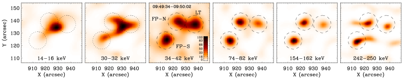
Figure 1.— Electron flux spectral images (with 8 keV bin width above 34 keV and 2 keV bin width at lower energies) up to 250 keV in the 2003 November 03 flare during the nonthermal peak as reconstructed from two sets of the regularized electron visibilities by the MEM_NJIT algorithm (Schmahl et al., 2007). The images show one LT and two FP sources above 34 keV and a loop structure at lower energies. Three circles are used to extract the LT and FP electron flux spectra above 34 keV (see Figure 2).

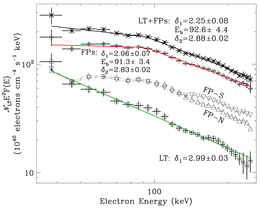
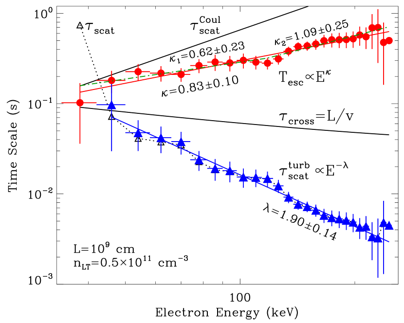
Figure 2.— Top: Electron power spectra ${\cal N}_{\rm LT}E^{2}F(E)$ for the LT (square), the two FPs summed (diamond), and all three sources (LT + FPs, cross) in the 2003 November 03 flare. The LT spectrum can be fitted by a power-law, and the summed FP and total spectra by a broken power-law. Also note that the southern FP spectrum (downward triangular) is flatter than the northern FP spectrum (upward triangular), mostly above $\sim$90 keV by $\sim$0.3 powers of energy, consistent with their asymmetric locations with respect to the LT. Bottom: Escape time (filled circle) and turbulence scattering time (filled triangular) in the (LT) acceleration region. The escape time can be well fitted by either a power-law or a broken power-law (dash dot) increasing with energy, and the turbulence scattering time by a power-law rapidly decreasing with energy. Also shown are the crossing, Coulomb scattering, and the mean scattering (open triangular) times. The reduced chi-squares for all the fittings are below or around 1.

3. Application: The 2003 November 03 Flare

As a first demonstration, we apply our new procedure to the 2003 November 03 solar flare (X3.9 class) during the nonthermal peak, in which we find a hard LT source (extending above 100 keV in HXR) distinct from the thermal loop in addition to two FP sources. In Figure 1 we show the electron flux images up to 250 keV, which also show a loop at low energies and one LT and two FPs at higher energies. In Figure 2 top panel we show the electron spectra ${\cal N}_{\rm LT}E^{2}F(E)$, where ${\cal N}_{\rm LT}=n_{\rm LT}L$ is the LT column density. The LT flux spectrum can be fitted by a power-law with an index $\delta_{\rm LT}=3.0$. The summed FP flux spectrum can be better fitted by a broken power-law with the indexes $\delta_{1}=2.1$ and $\delta_{2}=2.8$ below and above the break energy $E_{\rm b}=91\pm 3$ keV. It is clear that the total radiating electron spectrum differs significantly from the (LT) accelerated electron spectrum.

Given the above LT and FP electron flux spectra we derive the energy dependence of the escape time (eq. [7]). The LT density can be estimated as $n_{\rm LT}\simeq\sqrt{{\rm EM}/L^{3}}\simeq 0.5\times 10^{11}\ {\rm cm}^{-3}$, where the LT size $L\simeq 10^{9}$ cm is obtained from the LT angular size, and the emission measure ${\rm EM}\simeq 0.2\times 10^{49}$ cm^-3 is obtained from spectral fitting of the LT thermal emission. As in Figure 2 bottom panel, the escape time increases slowly with energy and can be fitted by either a power-law,

$$T_{\rm esc}(E)=0.3\ {\rm s}\left(\frac{E}{100\ {\rm keV}}\right)^{\kappa},\,\,\,\kappa=0.83\pm 0.10,$$ (8)

or a broken power-law with a break at $E_{\rm b}=118\pm 37$ keV, and the indexes $\kappa_{1}=0.62\pm 0.23$ and $\kappa_{2}=1.09\pm 0.25$. The fact that the escape time should be longer than the crossing time yields an upper limit on ${\cal N}_{\rm LT}$, which is satisfied by the above LT density and size.

We then calculate the mean scattering time in the LT region. Except at the lowest energy, the Coulomb contribution is small so that the scattering time thus calculated can be attributed to turbulence. The scattering time due to turbulence (see §2.3) can be fitted by a power-law above $\sim$40 keV,

$$\tau^{\rm turb}_{\rm scat}=0.016\ {\rm s}\left(\frac{E}{100\ {\rm keV}}\right)^{-\lambda},\,\,\,\lambda=1.90\pm 0.14.\,\,$$ (9)

4. Summary and Discussion

In this paper we describe a new method to directly obtain the model parameters for stochastic acceleration of particles by turbulence in solar flares from regularized inversion of the high resolution RHESSI HXR data (Piana et al., 2007). We have argued that particle acceleration takes place at or near the LT region. The accelerated electrons produce thin target emission at the LT and then escape downward to the dense FP region undergoing Coulomb collisions and producing thick target emission. In this model the LT and FP electron spectra are connected by the escape process from the LT region (eq. [6]), thus allowing us to determine the energy dependence of the escape time. Our method has the advantage that one can now constrain the model parameters uniquely rather than just satisfying the consistency between the model and the data as commonly done by forward fitting routines. This method can be applied to flares with simultaneous HXR emission from the LT and FP sources.

We have applied our method to the 2003 November 03 flare, in which we can obtain the electron flux images for both the LT and FPs up to 250 keV. The LT accelerated electron flux spectrum can be fitted by a power-law and the effective radiating flux spectrum at the FPs is better fitted by a broken power-law. From these spectra we derive the energy variation of the escape time and the scattering time. As seen in Figure 2, the turbulence scattering time is relatively short and decreases with energy. A short scattering time may arise from a high energy density of turbulence (${\cal E}_{\rm turb}$), with the exact relationship depending also on the magnetic field ($B$), and the spectral index ($q$) and minimum wave number ($k_{\rm min}$) of turbulence. A high level of turbulence also implies efficient acceleration which generally means a flat spectrum for the accelerated electrons, which is the case for the current flare. The energy dependences of $\tau^{\rm turb}_{\rm scat}$ and $D_{\rm EE}$ are also a function of these characteristics of turbulence; at high energies they are determined primarily by the spectral index of turbulence (see Dung & Petrosian, 1994; Pryadko & Petrosian, 1997, 1998, 1999; Liu et al., 2006).

For the usually assumed Kolmogorov ($q=5/3$) or Iroshnikov-Kraichnan ($q=3/2$) turbulence spectra, one expects the scattering time to increase with energy as $E^{2-q}$, which translates into an escape time varying roughly as $T_{\rm esc}\propto 1/\sqrt{E}$ at high (but non-relativistic) energies. The energy dependences of $T_{\rm esc}$ and $\tau^{\rm turb}_{\rm scat}$ obtained here require a steeper turbulence spectrum ($q>3$) at high wave numbers. Such a steep spectrum can be present beyond the inertial range where damping is important (e.g. Jiang et al., 2009). The electron energies and the wave-particle resonance condition determine the wave vector of the accelerating plasma waves. This relation depends primarily on the plasma parameter $\alpha\propto\sqrt{n}/B$ (e.g. Petrosian & Liu, 2004). Thus, given the magnetic field and plasma density we can determine the wave vectors for transition from the inertial to the damping ranges of turbulence.

It should, however, be emphasized that the results obtained here may not be representative of typical flares. More commonly flares have much softer LT emission, which would give an escape time decreasing (and scattering time increasing) with energy, consistent with a low level and a flat spectrum of turbulence.

The exact relation between the derived quantities ($N(E)$, $T_{\rm esc}$, and $\tau^{\rm turb}_{\rm scat}$) and the turbulence characteristics (${\cal E}_{\rm turb},B,q$, etc.) is complicated and depends on the angle of propagation of the plasma waves with respect to magnetic field and other plasma conditions. In future, we will apply these procedures to more flares (Q. Chen & V. Petrosian, 2010b, in preparation) and deal with these relations explicitly.

References

- Brown (1971) Brown, J. C. 1971, Sol. Phys., 18, 489
- Bykov & Fleishman (2009) Bykov, A. M., & Fleishman, G. D. 2009, ApJ, 692, L45
- Dingus et al. (1994) Dingus, B. L., et al. 1994, in AIP Conf. Proc. 294, High-energy Solar Phenomena, ed. J. M. Ryan & W. T. Vestrand (New York: AIP), 177
- Dung & Petrosian (1994) Dung, R., & Petrosian, V. 1994, ApJ, 421, 550
- Grigis & Benz (2006) Grigis, P. C., & Benz, A. O. 2006, A&A, 458, 641
- Hamilton & Petrosian (1992) Hamilton, R. J., & Petrosian, V. 1992, ApJ, 398, 350
- Holman et al. (2003) Holman, G. D., Sui, L., Schwartz, R. A., & Emslie, A. G. 2003, ApJ, 595, L97
- Hoyng et al. (1981) Hoyng, P., et al. 1981, ApJ, 246, L155
- Hudson (1972) Hudson, H. S. 1972, Sol. Phys., 24, 414
- Hurford et al. (2002) Hurford, G. J., et al. 2002, Sol. Phys., 210, 61
- Jiang et al. (2009) Jiang, Y. W., Liu, S., & Petrosian, V. 2009, ApJ, 698, 163
- Johns & Lin (1992) Johns, C. M., & Lin, R. P. 1992, Sol. Phys., 137, 121
- Koch & Motz (1959) Koch, H. W., & Motz, J. W. 1959, Rev. Mod. Phys., 31, 920
- Kontar et al. (2004) Kontar, E. P., Piana, M., Massone, A. M., Emslie, A. G., & Brown, J. C. 2004, Sol. Phys., 225, 293
- Lin & Schwartz (1987) Lin, R. P., & Schwartz, R. A. 1987, ApJ, 312, 462
- Lin et al. (2002) Lin, R. P., et al. 2002, Sol. Phys., 210, 3
- Liu et al. (2004) Liu, S., Petrosian, V., & Mason, G. M. 2004, ApJ, 613, L81
- Liu et al. (2006) Liu, S., Petrosian, V., & Mason, G. M. 2006, ApJ, 636, 462
- Liu et al. (2003) Liu, W., Jiang, Y. W., Petrosian, V., & Metcalf, T. R. 2003, Bulletin of the American Astronomical Society, 35, 839
- Marschhäuser et al. (1994) Marschhäuser, H., Rieger, E., & Kanbach, G. 1994, in AIP Conf. Proc. 294, High-energy Solar Phenomena, ed. J. M. Ryan & W. T. Vestrand (New York: AIP), 171
- Mason et al. (1986) Mason, G. M., Reames, D. V., von Rosenvinge, T. T., Klecker, B., & Hovestadt, D. 1986, ApJ, 303, 849
- Masuda et al. (1994) Masuda, S., Kosugi, T., Hara, H., Tsuneta, S., & Ogawara, Y. 1994, Nature, 371, 495
- Mazur et al. (1995) Mazur, J. E., Mason, G. M., & Klecker, B. 1995, ApJ, 448, L53
- Miller et al. (1996) Miller, J. A., Larosa, T. N., & Moore, R. L. 1996, ApJ, 461, 445
- Park et al. (1997) Park, B. T., Petrosian, V., & Schwartz, R. A. 1997, ApJ, 489, 358
- Petrosian (1973) Petrosian, V. 1973, ApJ, 186, 291
- Petrosian & Donaghy (1999) Petrosian, V., & Donaghy, T. Q. 1999, ApJ, 527, 945
- Petrosian et al. (2002) Petrosian, V., Donaghy, T. Q., & McTiernan, J. M. 2002, ApJ, 569, 459
- Petrosian et al. (2009) Petrosian, V., Jiang, Y. W., Liu, S., Ho, G. C., & Mason, G. M. 2009, ApJ, 701, 1
- Petrosian & Liu (2004) Petrosian, V., & Liu, S. 2004, ApJ, 610, 550
- Piana et al. (2007) Piana, M., Massone, A. M., Hurford, G. J., Prato, M., Emslie, A. G., Kontar, E. P., & Schwartz, R. A. 2007, ApJ, 665, 846
- Piana et al. (2003) Piana, M., Massone, A. M., Kontar, E. P., Emslie, A. G., Brown, J. C., & Schwartz, R. A. 2003, ApJ, 595, L127
- Pryadko & Petrosian (1997) Pryadko, J. M., & Petrosian, V. 1997, ApJ, 482, 774
- Pryadko & Petrosian (1998) Pryadko, J. M., & Petrosian, V. 1998, ApJ, 495, 377
- Pryadko & Petrosian (1999) Pryadko, J. M., & Petrosian, V. 1999, ApJ, 515, 873
- Ramaty (1979) Ramaty, R. 1979, in AIP Conf. Proc. 56, Particle Acceleration Mechanisms in Astrophysics, ed. J. Arons, C. McKee, & C. Max (New York: AIP), 135
- Schlickeiser (1989) Schlickeiser, R. 1989, ApJ, 336, 243
- Schmahl et al. (2007) Schmahl, E. J., Pernak, R. L., Hurford, G. J., Lee, J., & Bong, S. 2007, Sol. Phys., 240, 241