Removing Local Extrema from Imprecise Terrains

Abstract

In this paper we consider imprecise terrains, that is, triangulated terrains with a vertical error interval in the vertices. In particular, we study the problem of removing as many local extrema (minima and maxima) as possible from the terrain. We show that removing only minima or only maxima can be done optimally in $\color[rgb]{0.75,0.30,0.15}O(n\log n)$ time, for a terrain with $\color[rgb]{0.75,0.30,0.15}n$ vertices. Interestingly, however, removing both the minima and maxima simultaneously is NP-hard, and is even hard to approximate within a factor of $\color[rgb]{0.75,0.30,0.15}O(\log\log n)$ unless $\color[rgb]{0.75,0.30,0.15}\mathrm{P}=\mathrm{NP}$. Moreover, we show that even a simplified version of the problem where vertices can have only two different heights is already NP-hard, a result we obtain by proving hardness of a special case of 2-Disjoint Connected Subgraphs, a problem that has lately received considerable attention from the graph-algorithms community.

1 Introduction

Digital terrain analysis is an important part of geographical information science, with applications in hydrology, geomorphology, visualization, and many other fields [wg-tapa-98]. A popular structure for representing terrains is the triangulated irregular network (TIN), also known as polyhedral terrain. In this model, a terrain is represented by a planar triangulation with an additional height associated with each vertex. If we linearly interpolate the heights of the vertices, we also obtain a height at every other point in the plane, resulting in a bivariate, piecewise linear and continuous function, defining the surface of the terrain. A terrain in this model is also often called a 2.5-dimensional (or 2.5D) terrain.

1.1 Imprecision in Terrains

In computational geometry it is usually assumed that the input data for any problem is correct and known exactly. In practice, this is unfortunately not the case. There are many sources of imprecision, the most prominent of which is the data acquisition itself. In terrain modeling, this is particularly relevant, because elevation data is collected by measuring devices that are ultimately error-prone. Often such devices produce heights with a known error bound or return a height interval rather than a fixed height value.

In order to handle the imprecision in terrains, we adopt the model used in [ge-osp-04, gls-smit-10, ke-opsp-07], where the height of each terrain vertex is not precisely known, but only an interval of possible heights is available. This results in considerable freedom in the terrain, since the “real” terrain is unknown and any choice of a height for each vertex—as long as it is within its height interval—leads to a valid realization of the imprecise terrain. The large number of different realizations of an imprecise terrain leads naturally to the problem of finding one that is ‘best’ according to some criterion, or that removes most or many instances of a certain type of unwanted feature (or artifact) from the terrain.

We note that, even though terrain data may contain error also in the $\color[rgb]{0.75,0.30,0.15}x,y$-coordinates, under this model we consider imprecision only in the $\color[rgb]{0.75,0.30,0.15}z$-coordinate. This simplifying assumption is justified by the fact that error in the $\color[rgb]{0.75,0.30,0.15}x,y$-coordinates will most likely produce elevation error. Moreover, often the data provided by commercial terrain data suppliers only reports the elevation error [ft-ccedem-06].

In the remainder of this paper, an imprecise terrain is a set of $\color[rgb]{0.75,0.30,0.15}n$ vertical intervals in $\color[rgb]{0.75,0.30,0.15}\mathbb{R}^{3}$, together with a triangulation of the vertical projection. Figure 1 shows an example. A realization of an imprecise terrain is a triangulated terrain that has the same triangulation in the projection, and exactly one vertex on each interval. An alternative way to view an imprecise terrain is by connecting the tops of all intervals into a terrain, which we call the ceiling, and the bottoms into a second terrain, which we call the floor. Then, a realization is a terrain that lives in the space left open between the floor and the ceiling. Figure 1 shows this in the example.

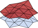
Figure 1: (a) An example of an imprecise terrain. (b) The same terrain, shown by drawing the floor and the ceiling.

1.2 Removing local extrema

A local minimum (or pit) is a location on a terrain that is surrounded by higher points, or that has no lower neighboring point. Similarly, a local maximum (or peak) is as a point surrounded by lower points or without higher neighbors. The term local extrema will be used to refer to both local minima and local maxima.

When terrains are used for land erosion, landscape evolution, or hydrological studies, it is generally accepted that the majority of local extrema in the terrain model are spurious, caused by errors in the data or model production. A terrain model with many pits or peaks does not represent the terrain faithfully, and moreover, in the case of pits, it can create problems because water accumulates at them, affecting water flow routing simulations. For this reason the removal of local minima from terrain models is a standard preprocessing requirement for many uses of terrain models [ztz-edpah-06, tsv-adddl-06]. However, existing preprocessing routines make no attempt to relate the removed minima to knowledge about the imprecision in the terrain model, possibly causing major alterations to the data under study.

In this paper we attempt to solve the problems of removing as many local minima, maxima, or extrema as possible by moving the vertices of an imprecise terrain within their allowed height intervals. The rationale behind this is that if a pit (or peak) can be removed in this way, it is likely to be an artifact of the data, whereas if it cannot, it is more certain to be a ‘real’ pit (or peak). We define the minimizing-minima, the minimizing-maxima, and the minimizing-extrema problems on imprecise terrains, where we attempt to find a realization of an imprecise terrain (by placing the imprecise points within their intervals) that minimizes the number of local minima, local maxima, and local extrema, respectively.

It is important to note that a group of $\color[rgb]{0.75,0.30,0.15}k$ connected vertices at the same height without any lower neighbor is considered to be only one local minimum. This is reasonable from the point of view of the application, and follows the definitions used in previous work [so-fcdd-07]. In Section LABEL:sec:degeneracy we discuss what the implications of this modeling choice are for our results.

Regarding previous work, a lot of research has been devoted to the problem of removing local minima from (precise) terrains, especially in the geographic information science community, but also from more algorithmic points of view; we only provide a few relevant references here. Most of the literature assumes a raster (grid) terrain (e.g. [m-nmg-88, mg-aobat-99, ztz-edpah-06]), and employs methods that are some type of “pit filling” technique, which consist in filling in depressions until they disappear (e.g. [cdp-qafdn-00, m-nmg-88, ztz-edpah-06]). Some of the few exceptions are the methods in [cd-bdgt-10, mg-aobat-99, r-pbauca-98]. A few algorithms have been proposed for triangulated terrains, such as [ls-ftt-04, aay-ioebu-06]. The removal of local extrema has also been studied in the context of optimal higher order Delaunay triangulations [ghk-hodt-02, kkl-grtho-07]. In particular, Gudmundsson et al. [ghk-hodt-02] show that the optimal number of both local minima and local maxima can be removed from first-order Delaunay triangulations in $\color[rgb]{0.75,0.30,0.15}O(n\log n)$ time. More related to this paper, Silveira and Van Oostrum [so-fcdd-07] study moving vertices vertically in order to remove all local minima with a minimum cost, but do not assume bounded intervals.

1.3 Results

In Section 2, we first study the problem of finding a realization of an imprecise terrain that minimizes the number of local minima (or local maxima). We show that all potential local minima (resp. maxima) of the terrain are independent, that is, whether we remove one does not influence whether or not we can remove another. Using this property, we then present a relatively simple algorithm that removes local minima (maxima) optimally in $\color[rgb]{0.75,0.30,0.15}O(n\log n)$ time.

In Section 3, we turn our attention to removing both minima and maxima simultaneously. In this case we no longer have the independence property, and as a consequence the problem becomes much harder. In fact, we show that the problem of minimizing the total number of local extrema is NP-hard, even hard to approximate within a factor $\color[rgb]{0.75,0.30,0.15}O(\log\log n)$ unless $\color[rgb]{0.75,0.30,0.15}\mathrm{P}=\mathrm{NP}$.

All results mentioned above assume general position of the input (that is, all the top and bottom ends of the intervals have different heights), and considers points chosen to be at the same height as a group to be at most one single local extremum. In Section LABEL:sec:degeneracy, we discuss how these assumptions influence the results presented in Section 3.

Finally, in Section LABEL:sec:intermezzo, we consider a simplified version of the problem of removing local extrema, where grobally all vertices of a terrain have only two possible heights. We show that this problem is already NP-hard, and cannot be approximated within a factor $\color[rgb]{0.75,0.30,0.15}3/2$. For this, we prove that the planar version of 2-Disjoint Connected Subgraphs is NP-hard. The latter problem has received quite some attention recently, and we consider the connection this hardness proof to be of independent interest.

2 Removing local minima

We begin with the problem of finding a realization that has the smallest number of local minima, that is, the minimizing-minima problem. We propose an efficient algorithm based on the idea of selectively flooding parts of the terrain. The algorithm begins with all vertices as low as possible, and simulates flooding parts of the terrain.

Algorithm

Conceptually, we raise all local minima as much as possible, that is, we raise each minimum and its neighbors as we meet them, merging minima as we sweep the terrain bottom-up. The process stops when one of the vertices in a local minimum cannot be raised any further. Also, when there is only one local minimum left and no more higher terrain it could merge into, the process stops.

We sweep a horizontal plane vertically, starting at the lowest interval end and moving upwards in the $\color[rgb]{0.75,0.30,0.15}z$ direction. As the plane moves up, it pulls some of the vertices with it, whose height is changing together with the plane. At any moment during the sweep, each vertex is in one of three states:

1. Moving, if it is currently part of a local minimum, and is moving up together with the sweep plane.

2. Fixed, at a height lower than the current one.

3. Unprocessed, if it has not been reached by the sweep plane yet.

As the sweep plane moves vertically up, we distinguish two types of events:

1. The plane reaches the beginning (lowest end) of the interval of a vertex,

2. The plane reaches the end (highest end) of the interval of a vertex.

Let $\color[rgb]{0.75,0.30,0.15}v$ denote the vertex whose interval just began or ended, and let $\color[rgb]{0.75,0.30,0.15}h$ be the current height of the plane. Note that all fixed vertices are fixed at a height lower than $\color[rgb]{0.75,0.30,0.15}h$.

An event of type (i) can create a number of situations.

If $\color[rgb]{0.75,0.30,0.15}v$ has a neighbor that is already fixed, then $\color[rgb]{0.75,0.30,0.15}v$ will never be a local minimum, thus $\color[rgb]{0.75,0.30,0.15}v$ is fixed at its lowest possible height. Moreover, if some other neighbor of $\color[rgb]{0.75,0.30,0.15}v$ is currently part of a local minimum (i.e. is moving), then all the vertices part of that local minimum become fixed at $\color[rgb]{0.75,0.30,0.15}h$, and automatically stop being a minimum. This occurs for each neighbor of $\color[rgb]{0.75,0.30,0.15}v$ that is currently part of a local minimum.

If all neighbors of $\color[rgb]{0.75,0.30,0.15}v$ are currently unprocessed, then $\color[rgb]{0.75,0.30,0.15}v$ becomes a new local minimum, and starts to move up together with the plane.

Finally, if no neighbor is fixed but some neighbor is moving, thus is part of a local minimum, then $\color[rgb]{0.75,0.30,0.15}v$ will join that existing local minimum and also start to move up together with the plane (note that if there is more than one local minimum that is connected to $\color[rgb]{0.75,0.30,0.15}v$, at this step they all merge into one).

Events of type (ii), when an interval ends, are easier to handle. If $\color[rgb]{0.75,0.30,0.15}v$ is fixed, nothing occurs. If $\color[rgb]{0.75,0.30,0.15}v$ was moving, then it becomes fixed at $\color[rgb]{0.75,0.30,0.15}h$, and the same occurs to all the vertices of the local minimum that contains $\color[rgb]{0.75,0.30,0.15}v$. Thus the whole local minimum becomes fixed, and will be present in the final solution.

Correctness

The correctness of the algorithm can be proved by induction on the steps (i.e. events) of the sweep (associated with exactly $\color[rgb]{0.75,0.30,0.15}2n$ height values). Let $\color[rgb]{0.75,0.30,0.15}h_{i}$ denote the height of the plane at the $\color[rgb]{0.75,0.30,0.15}i$th event. Clearly, for $\color[rgb]{0.75,0.30,0.15}h=h_{1}$ the terrain processed has only one local minimum, comprised of the lowest vertex, which is optimal. Now assume that for $\color[rgb]{0.75,0.30,0.15}h=h_{i}$ the solution is optimal. That is, the number of local minima in the imprecise terrain resulting from cropping the original terrain $\color[rgb]{0.75,0.30,0.15}T$ by the plane at height $\color[rgb]{0.75,0.30,0.15}h_{i}$ (that is, $\color[rgb]{0.75,0.30,0.15}T\cap(z\leq h_{i})$) is minimum.

We analyze the type of event that can take place for $\color[rgb]{0.75,0.30,0.15}h=h_{i+1}$. Let $\color[rgb]{0.75,0.30,0.15}v$ be the vertex whose interval is ending or beginning at $\color[rgb]{0.75,0.30,0.15}h=h_{i+1}$.

If the interval of $\color[rgb]{0.75,0.30,0.15}v$ is ending, then $\color[rgb]{0.75,0.30,0.15}v$ is part of a local minimum that will be fixed. Since this local minimum already existed in the previous step, and that solution was optimal by the inductive hypothesis, the current solution is also optimal.

If the interval of $\color[rgb]{0.75,0.30,0.15}v$ is just starting, it is only necessary to argue about the optimality of the connected component (induced by the vertices in the cropped terrain) that contains $\color[rgb]{0.75,0.30,0.15}v$. The other connected components are optimal due to the inductive hypothesis, because they have not changed by this event.

Consider first the case in which $\color[rgb]{0.75,0.30,0.15}v$ is connected to at most one fixed (lower) local minimum in the current cropped terrain. Then the connected component that contains $\color[rgb]{0.75,0.30,0.15}v$ will end up consisting of a single local minimum. Since every connected component has at least one local minimum, this is optimal for the component that contains $\color[rgb]{0.75,0.30,0.15}v$.

In case that $\color[rgb]{0.75,0.30,0.15}v$ is connected to more than one lower local minimum, we note that none of them can be removed by connecting them to $\color[rgb]{0.75,0.30,0.15}v$, because the lowest possible position for $\color[rgb]{0.75,0.30,0.15}v$ is at $\color[rgb]{0.75,0.30,0.15}h_{i+1}$, which is higher than all its neighbors (recall that, by construction, fixed local minima are at their highest possible height). Therefore in this case the number of local minima for the connected component that contains $\color[rgb]{0.75,0.30,0.15}v$ stays the same, leading again to an optimal solution for that component. Therefore the current cropped terrain has the minimum possible number of local minima, and the correctness of the algorithm follows.

Finally, $\color[rgb]{0.75,0.30,0.15}v$ can become connected to one or more vertices that were moving (thus were part of one or more local minima). In this case, they all become one single (moving) connected component, connected through $\color[rgb]{0.75,0.30,0.15}v$, and hence one single local minima. Again, this is optimal for that component.

Running time

Sorting the interval ends for the sweep requires $\color[rgb]{0.75,0.30,0.15}O(n\log n)$ time. We put the ends in an event queue and mark each event as either of type (i) or type (ii). We remove all events of type (ii) that come after the last event of type (i).

The rest of the steps can be implemented in linear time as follows. For every vertex, we simply maintain a label that has a value of either moving, fixed or unprocessed.

At an event of type (i) where the sweep plane reaches the bottom of an unprocessed vertex $\color[rgb]{0.75,0.30,0.15}v$, we first inspect all neighbours of $\color[rgb]{0.75,0.30,0.15}v$ to determine which subcase we are in. This takes time proportional to the number of neighbours, and we charge this cost to the edges connecting $\color[rgb]{0.75,0.30,0.15}v$ to its neighbours. Since we charge each edge at most twice over the whole algorithm, this takes linear time in total. Now, if no neighbour of $\color[rgb]{0.75,0.30,0.15}v$ is fixed, we simply set the label of $\color[rgb]{0.75,0.30,0.15}v$ to moving in constant time. If some neighbour of $\color[rgb]{0.75,0.30,0.15}v$ is fixed, we set the label of $\color[rgb]{0.75,0.30,0.15}v$ to fixed, and we start a floodfill (for example using a depth first search) in the graph induced by the moving vertices to find all vertices connected to $\color[rgb]{0.75,0.30,0.15}v$ that are currently set to moving; we set them to fixed as well, and we set their height to the current height of the sweep plane. This takes time proportional to the number of vertices that are being fixed plus the number of edges connecting these vertices to other vertices. Since each vertex gets fixed only once, this also amounts to linear work in total.

Events of type (ii) are handled similarly. If $\color[rgb]{0.75,0.30,0.15}v$ was moving, we set its label to fixed and also start the floodfill in the same way.

When all events in the queue have been processed, we finally set the remaining moving vertices to fixed as well.

Note that by multiplying all interval ends with $\color[rgb]{0.75,0.30,0.15}-1$, we can solve also the minimizing-maxima problem.

Theorem 1

The minimizing-minima (or minimizing-maxima) problem in an imprecise terrain with $\color[rgb]{0.75,0.30,0.15}n$ vertices can be solved in $\color[rgb]{0.75,0.30,0.15}O(n\log n)$ time.

It is interesting to note that when a group of $\color[rgb]{0.75,0.30,0.15}k$ connected vertices at the same height without any lower neighbors is regarded as $\color[rgb]{0.75,0.30,0.15}k$ different local minima, the problem can be proved NP-hard. More details on this are given in Section LABEL:sec:degeneracy.

3 Removing all local extrema

We now move on to the problem of removing all local extrema at the same time. Although the algorithm in the previous section works for both removing minima and removing maxima, it is not possible to use both height assignments simultaneously. We will show in the next section that we can still use the algorithm twice to narrow down the problem, without changing the value of the solution. Unfortunately, such an approach does not help much to find an optimal realization minimizing the number of maxima. In Section 3.2 we give a proof that shows that minimizing-extrema is NP-hard to approximate within a factor of $\color[rgb]{0.75,0.30,0.15}O(\log\log n)$, using a reduction from Set Cover.

3.1 Canonical form of an imprecise terrain

Recall that the floor $\color[rgb]{0.75,0.30,0.15}F$ is the realization formed by all lower endpoints of the imprecise vertices, and the ceiling $\color[rgb]{0.75,0.30,0.15}C$ is the realization formed by all upper endpoints, as shown in Figure 1.

Given two realizations $\color[rgb]{0.75,0.30,0.15}X$ and $\color[rgb]{0.75,0.30,0.15}Y$ of the same imprecise terrain, we use the notation $\color[rgb]{0.75,0.30,0.15}(X,Y)$ to refer to the imprecise terrain truncated by $\color[rgb]{0.75,0.30,0.15}X$ and $\color[rgb]{0.75,0.30,0.15}Y$: the bottom interval ends are taken from the heights in $\color[rgb]{0.75,0.30,0.15}X$, and the top interval ends from the heights in $\color[rgb]{0.75,0.30,0.15}Y$ (we assume here that $\color[rgb]{0.75,0.30,0.15}X$ is never above $\color[rgb]{0.75,0.30,0.15}Y$).

We are searching for a surface between the floor and the ceiling that optimizes the number of local extrema. We will run the algorithm in Section 2 on $\color[rgb]{0.75,0.30,0.15}(F,C)$ to remove the local minima, and call the result $\color[rgb]{0.75,0.30,0.15}F^{\prime}$, and run it again on $\color[rgb]{0.75,0.30,0.15}(F,C)$ to remove local maxima and call the result $\color[rgb]{0.75,0.30,0.15}C^{\prime}$. We call the imprecise terrain $\color[rgb]{0.75,0.30,0.15}(F^{\prime},C^{\prime})$ the canonical form of $\color[rgb]{0.75,0.30,0.15}(F,C)$.

Lemma 1

The imprecise terrain induced by $\color[rgb]{0.75,0.30,0.15}(F^{\prime},C^{\prime})$ is still a valid imprecise terrain which has the same optimal solution for removing local extrema as the original terrain $\color[rgb]{0.75,0.30,0.15}(F,C)$.

Proof 3.2.

We need to show two things. To show that $\color[rgb]{0.75,0.30,0.15}(F^{\prime},C^{\prime})$ is still a valid imprecise terrain, we need that the height of any vertex in $\color[rgb]{0.75,0.30,0.15}F^{\prime}$ is at least the height of that vertex in $\color[rgb]{0.75,0.30,0.15}C^{\prime}$. If there exists a height $\color[rgb]{0.75,0.30,0.15}h$ such that the entire floor lies below $\color[rgb]{0.75,0.30,0.15}h$ and the entire ceiling lies above $\color[rgb]{0.75,0.30,0.15}h$, then neither of them will ever raise/lower beyond $\color[rgb]{0.75,0.30,0.15}h$, because of the stop condition when there are no new interval events anymore. Otherwise, if a vertex $\color[rgb]{0.75,0.30,0.15}v$ does not rise higher this is because its plateau hits a point of the ceiling; clearly a plateau lowering $\color[rgb]{0.75,0.30,0.15}v$ will never move past this point. In both cases, a plateau rising the floor and one lowering the ceiling of the same vertex never cross each other.

To show that $\color[rgb]{0.75,0.30,0.15}(F^{\prime},C^{\prime})$ has the same optimal solution as $\color[rgb]{0.75,0.30,0.15}(F,C)$, we need to show that there exists an optimal terrain $\color[rgb]{0.75,0.30,0.15}T^{*}$ between $\color[rgb]{0.75,0.30,0.15}F$ and $\color[rgb]{0.75,0.30,0.15}C$ that in fact also lies between $\color[rgb]{0.75,0.30,0.15}F^{\prime}$ and $\color[rgb]{0.75,0.30,0.15}C^{\prime}$. This is true because if a terrain would have a local minimum below $\color[rgb]{0.75,0.30,0.15}F^{\prime}$, we could freely lift it together with its neighbors until it coincides with $\color[rgb]{0.75,0.30,0.15}F^{\prime}$. By the construction of $\color[rgb]{0.75,0.30,0.15}F^{\prime}$, we never hit the ceiling during this process, so we never increase the number of minima or maxima. The converse is true for local maxima above $\color[rgb]{0.75,0.30,0.15}C^{\prime}$.

Lemma 1 implies that we can run the algorithm of Section 2 as a preprocessing step, while still allowing a solution as good as in the original problem. Furthermore, the canonical terrain has more structure than the original one. Every remaining local minimum of the floor touches the ceiling, and every remaining local maximum of the ceiling touches the floor. We can show the following:

Lemma 3.3.

The total number of extrema in the optimal solution $\color[rgb]{0.75,0.30,0.15}T^{*}$ is never greater than the number of local maxima of the floor $\color[rgb]{0.75,0.30,0.15}F^{\prime}$ + the number of local minima of the ceiling $\color[rgb]{0.75,0.30,0.15}C^{\prime}$.

Proof 3.4.

Consider the solution $\color[rgb]{0.75,0.30,0.15}T=C^{\prime}$. Any local maximum of $\color[rgb]{0.75,0.30,0.15}T$ must touch a unique local maximum of $\color[rgb]{0.75,0.30,0.15}F^{\prime}$ because when lowering the maxima of $\color[rgb]{0.75,0.30,0.15}C$ this was exactly the condition on which we stopped. Therefore, the number of local maxima of $\color[rgb]{0.75,0.30,0.15}T$ is smaller than the number of local maxima of $\color[rgb]{0.75,0.30,0.15}F^{\prime}$. Thus, the number of local extrema in $\color[rgb]{0.75,0.30,0.15}T$ is at most the number of local maxima of $\color[rgb]{0.75,0.30,0.15}F^{\prime}$ + the number of local minima of $\color[rgb]{0.75,0.30,0.15}C^{\prime}$ (which is $\color[rgb]{0.75,0.30,0.15}T$ itself). Clearly, the number of local extrema in the optimal solution $\color[rgb]{0.75,0.30,0.15}T^{*}$ can only be even smaller.

If we denote by $\color[rgb]{0.75,0.30,0.15}\mathrm{lmin}(T)$ the number of local minima in a terrain $\color[rgb]{0.75,0.30,0.15}T$ and by $\color[rgb]{0.75,0.30,0.15}\mathrm{lmax}(T)$ the number of local maxima in $\color[rgb]{0.75,0.30,0.15}T$, and we denote by $\color[rgb]{0.75,0.30,0.15}T^{*}$ the optimal solution of our problem $\color[rgb]{0.75,0.30,0.15}(F,C)$, then we can summarize these observations as follows:

$$\mathrm{lmin}(F^{\prime})+\mathrm{lmax}(C^{\prime})\leq\mathrm{lmin}(T^{*})+\mathrm{lmax}(T^{*})\leq\mathrm{lmin}(C^{\prime})+\mathrm{lmax}(F^{\prime})$$ (1)

This formula gives a bound on the values of a particular instance. In theory, the gap may still be arbitrarily large. For example, consider an instance where the floor is more or less flat except for a number of “stalagmites” that reach all the way to the ceiling, and the ceiling is more or less flat except for a number of “stalactites” that reach all the way to the floor. Figure 2 show such a situation.

Remark 3.5.

MaartensaysI liked the old spikes figure a little better than this one, but I don’t mind too much either way. (Which one is ”correct” depends on whether we look at the surface as being smooth or having a sharp angle at the base of the cones. I was originally going for the smooth look.) In this case, the number of maxima of the floor and minima of the ceiling is large, while the floor has only a single minimum and the ceiling has only a single maximum, and the preprocessing step will not make a difference. We see in the next section that this makes the problem very hard to solve.

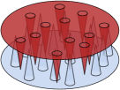
Figure 2: An imprecise terrain that has many maxima on the floor and many minima on the ceiling.

On the other hand, such terrains seem unlikely to appear in real applications. It may be likely that in practice, the gap in Equation 1 is quite small. Under which properties of terrains this is the case remains an interesting open question.

3.2 Hardness of approximation

In this section we show by a direct reduction from the Set Cover problem that we cannot approximate the number of local extrema on $\color[rgb]{0.75,0.30,0.15}n$-vertex graphs within any factor better than $\color[rgb]{0.75,0.30,0.15}O(\log\log n)$ unless $\color[rgb]{0.75,0.30,0.15}\mathrm{P}=\mathrm{NP}$.

Given a tuple $\color[rgb]{0.75,0.30,0.15}(U,C)$, where $\color[rgb]{0.75,0.30,0.15}U$ is a finite set called universe and $\color[rgb]{0.75,0.30,0.15}C$ is a collection of subsets of $\color[rgb]{0.75,0.30,0.15}U$ with $\color[rgb]{0.75,0.30,0.15}\bigcup_{S\in C}S=U$, a set cover for $\color[rgb]{0.75,0.30,0.15}(U,C)$ is a collection $\color[rgb]{0.75,0.30,0.15}C^{\prime}\subseteq C$ such that the union of all sets in $\color[rgb]{0.75,0.30,0.15}C^{\prime}$ is equal to $\color[rgb]{0.75,0.30,0.15}U$. The size of $\color[rgb]{0.75,0.30,0.15}C^{\prime}$ is its cardinality. The Set Cover problem is to find a set cover of minimal size.

Let $\color[rgb]{0.75,0.30,0.15}(U,C)$ be an instance of the Set Cover problem. We start by defining a graph $\color[rgb]{0.75,0.30,0.15}G$ with colored vertices. We then construct a terrain by embedding $\color[rgb]{0.75,0.30,0.15}G$ in the plane, and triangulating its faces with more than 3 incident vertices. Finally, we assign heights to the terrain vertices, where the height of every vertex depends on its color.

In the remainder, we will use the terms west and east to refer to the negative and positive $\color[rgb]{0.75,0.30,0.15}x$-direction, south and north to refer to the negative and positive $\color[rgb]{0.75,0.30,0.15}y$-direction, and down and up to refer to the negative and positive $\color[rgb]{0.75,0.30,0.15}z$-direction.