Bandgaps and band bowing in semiconductor alloys

Abstract

The bandgap and band bowing parameter of semiconductor alloys are calculated with a fast and realistic approach. The method is a dielectric scaling approximation that is based on a scissor approximation. It adds an energy shift to the bandgap provided by the local density approximation (LDA) of the density functional theory (DFT). The energy shift consists of a material-independent constant weighted by the inverse of the high-frequency dielectric constant. The salient feature of the approach is the fast calculation of the dielectric constant of alloys via the Green function (GF) of the TB-LMTO (tight-binding linear muffin-tin orbitals) in the atomic sphere approximation (ASA). When it is applied to highly mismatched semiconductor alloys (HMAs) like Zn Te_x Se_1-x, this method provides a band bowing parameter that is different from the band bowing parameter calculated with the LDA due to the bowing exhibited also by the high-frequency dielectric constant.

1 Introduction

Semiconductor alloying is a very important way of bandgap engineering with applications in tailoring the materials properties like the electronic stucture or optical behaviour. The bandgap of semiconductor alloys can be usually described by a quadratic polynomial in concentration $x$ with the quadratic coefficient being called the bowing coefficient. Accordingly, the bandgap $E_{g}$ of an alloy AB_xC_1-x is described by

$$E_{g}(x)=xE_{g}(AB)+(1-x)E_{g}(AC)-bx(1-x),$$ (1)

where $E_{g}(AB)$ and $E_{g}(AC)$ are the bandgaps of the binary constituents $AB$ and $AC$. The bandgap bowing coefficient $b$ describes the deviation from linearity and is close to a constant for most alloys.

Highly mismatched semiconductor alloys (HMAs) exhibit a large bowing parameter. HMAs are present in III-V systems like Ga N_x As_1-x [1], Ga Bi_x As_1-x, and Ga Sb_x As_1-x [2]; II-VI compounds like Zn S_x Te_1-x [3], Zn Te_x Se_1-x[4], and Zn O_x Te_1-x [5]; and IV-IV alloys like Sn_x Ge_1-x [6]. Lattice relaxation, localization, charge transfer, and huge bandgap bowing are encountered in HMA systems due to large differences in atomic sizes and orbital energies, and large lattice mismatch.

The bandgap bowing of HMAs cannot be described well by simple models like virtual crystal approximation, at least in the mid-alloy regime of concentrations [7]. Other models like the band anticrossing (BAC) model [1], the valence-band anticrossing (VBAC) models [2] or combinations of them [4, 8] are able to explain the strong bandgap change with concentration $x$. These models are applied in the dilute limit of concentrations, in which one constituent is considered as an impurity with composition-dependent coupling to the conduction band minimum or valence band maximum. However, the BAC model and its extensions completely neglect cluster states induced by impurities [9]. Supercell methods overcome this shortcoming but the price is large unit cells [10]. More efficient approaches are based on special quasirandom structures (SQSs) having smaller supercells in which the most relevant atom-atom correlation functions are similar to those of random alloys [11].

Standard first-principles band theory is based on the Kohn-Sham (KS) scheme [12] of the density functional theory (DFT) [13], which is, in principle, exact. The DFT is a total-energy method for calculating the electronic ground state. The local density approximation (LDA) [13] and the generalized gradient approximation (GGA) [14] provide reasonably accurate results for ground-state properties like crystal structure, pressure-induced transformations, phonon spectra, magnetism, etc. Usually the LDA leads to some overbindings. For example, in materials, where narrow bands determined by semi-core states (for instance, Zn 3d states in ZnSe and ZnTe) contribute to the bonding, the LDA predicts these localized semi-core states too high in energy. In addition, the LDA and GGA do not describe well the long-range part of correlations and have the so-called ”bandgap problem”. Even though the LDA often yields good band dispersions for the valence bands, the LDA bandgap energy in semiconductors and insulators is much smaller than the experimental bandgap. The theory that may solve that problem is the Hedin’s GW approximation (GWA: $G=$ Green function and $W=$ screened Coulomb interaction) [15, 16, 17]. The corrections in the GWA are provided by the self-energy that resembles the Hartree-Fock exchange term, which is a non-local operator. Fortunately the eigenvectors obtained with the Hartree-Fock approximation (HFA), the LDA, and the GWA are often very close [18, 19]. Therefore, in many cases one can obtain good results with the GWA by solving first the LDA problem, and then taking the expectation value of the GWA self-energy over the LDA eigenvectors.

The calculations in the GWA are based on the screening of the exchange interaction with the inverse frequency-dependent dielectric matrix as opposed to local exchange-correlation potentials in the LDA. The computational cost, however, is large due to the evaluation of dielectric matrices, their inversion, etc. Thus, the GWA is usually restricted to relatively small systems. One way to circumvent these computational hurdles is to use dielectric function models [20, 21] and dielectric models such as Thomas-Fermi screening in the screened-exchange LDA (SX-LDA) methods [22, 23]. Although these schemes are computationally ”cheaper” than the GWA, only quite recently have SX-LDA methods been used to larger systems [24, 25]. Moreover, despite the fact that these methods provide a much better description of the bandgaps than the LDA, it appears that it is rather difficult to define the screening constants of alloys.

Generally, in the HMA the bandgap bowing coefficient is composition dependent, reflecting the strong wave-function localization at the band edges (see [4] and the references therein). In such materials there is a strong interaction between the band edge states and localized, impurity-like states in alloys. To be explicit, in semiconductor alloys like ZnTe_xSe_1-x there is a strong interaction between the localized Te level and the valence band of the host in the Se-rich limit of concentrations. On the other hand, in the Te-rich limit of concentrations there is a strong coupling between localized Se level and the conduction band. Because the bowing coefficient is calculated as a variation, i.e., a difference that enables some cancellations, the LDA would seem appropriate, at least in a zero-order approximation. In alloys like ZnTe_xSe_1-x, however, the use of the LDA has two major caveats. The first is related to the underestimation of the bandgap and the height of the conduction band. The second comes from the overbinding of the cation d states that mix too much with p states of the valence band maximum and push these p states upward in energy. Thus, in HMA the LDA would rather fail to have realistic assessment of not only the bandgap but also the band bowing over the whole range of alloy composition $x$. Below, we present a fast and simple method that estimates the bandgap and band bowing coefficient with an accuracy approaching that of more demanding methods like the GWA and SX-LDA. The concrete example of ZnTe_xSe_1-x is analyzed and discussed.

2 Method

There is still a simpler method to calculate the semiconductor bandgaps. It is based on the scissor operator [16] and is basically a dielectric scaling approximation (DSA) for correcting the LDA bandgaps [26]. Thus for a wide variety of materials the main correction to the LDA bandgap is [26]

$$\Delta\simeq\frac{\alpha}{\varepsilon_{\infty}},$$ (2)

where $\alpha=9.1$ eV is a universal constant and $\varepsilon_{\infty}$ is the high-frequency dielectric constant of the material. The method is applied not only to usual zinc blende or wurtzite types but also to other structures like technologically interesting high-dielectric materials [27]. Beside the technical arguments presented in the original paper [26] there are other arguments that ensure the success of this method. First, there is the perturbative argument of the GWA with respect the LDA [18]: the GWA corrections are basically the expectation value of the GW self-energy over the LDA eigenvectors. Second, the difference between quasiparticle energies and the LDA eigenvalues is essentially due to the non-local nature of the effective potential [28], which can be expressed with a scissor-like operator [26]. There is also a more physical picture provided by Harrison [29]. The exact non-local exchange operator of the Hartree-Fock theory has a long-range part which is unscreened, and hence overestimated. In the LDA the exchange operator is replaced by a local exchange-correlation operator which neglects the long-range part of the exchange altogether. In semiconductors the long-range part of the exchange is screened by the high-frequency dielectric constant. The LDA uses a fixed one-electron potential for all bands including the unoccupied bands. Thus the LDA neglects the electrostatic energy $U$ needed for the separation of the electron and hole in the excitation that provides the bandgap. Harrison noted that the excitation process is accompanied by a dielectric relaxation around the electron and the hole such that the correction to the bandgap is a rigid shift for the entire conduction band of order $U/\varepsilon_{\infty}$. Finally, a quite similar approach has been reported recently. It starts from the optimized effective potential method with a free parameter, whose value is established by the separation between the short-ranged and long-ranged exchange in the screened hybrid functional [30].

In the present work we calculate the bandgap and band bowing coefficient in semiconductor alloys beyond the LDA by calculating the high-frequency dielectric constant. The equilibrium positions of atoms in the SQS supercells representing the alloy are determined with the Vienna ab initio simulation package (VASP) [31] with the projector augmented-wave method (PAW) [32]. Then the electronic structure is calculated with the tight-binding (TB) linear muffin-tin orbital method (LMTO) in its atomic sphere approximation (ASA) [33, 34, 35] in the LDA. The TB-LMTO-ASA method is one of the most efficient, versatile, and also one of the most physically transparent methods. Other methods use a bigger number of basis functions and they are usually more difficult to interpret physically. Even though it uses the shape approximation (the Wigner-Seitz (WS) cells are replaced by overlapping WS spheres), the TB-LMTO-ASA method is quite successful in the description of closely packed solids, whereas empty spheres are used in the interstitial region to close pack open structures [36]. As a rule, the shape approximation does quite well for closely packed systems, in particular for energy bands, but not that well for total energy calculations. Finally the static polarization $\chi^{0}$ and the high-frequency dielectric constant $\varepsilon_{\infty}$ are calculated with the TB-LMTO-ASA. The procedure is laid out below.

Let us then consider the static screening of a test charge in the random phase approximation [16]. Consider a lattice of points (spheres), with the electron density in equilibrium. We wish to calculate the response (screening) in the electron charge $\delta q_{j}$ at site $j$, induced by the addition of a small external potential $\delta V_{i}$ at site $i$. The electron charge $\delta q_{j}$ is related to $\delta V_{i}$ by the non-interacting response function $\chi_{ij}^{0}$:

$$\delta q_{i}^{0}\equiv\chi_{ij}^{0}\delta V_{j}.$$ (3)

$\chi_{ij}^{0}$ can be calculated in the first-order perturbation theory from the eigenvectors of a non-interacting one-electron Schrödinger equation with the Adler-Wiser formalism [37, 38] or directly via $G^{0}$, the Green function (GF) calculated from the one-electron Hamiltonian of the LDA. By linearizing the Dyson equation for the perturbed GF, i. e. $\delta G=G^{0}\delta VG\approx G^{0}\delta VG^{0}$, one obtains an explicit representation of $\chi_{ij}^{0}$ in terms of $G^{0}$

$$\begin{array}[]{l}\delta q_{i}^{0}=\frac{1}{\pi}\mbox{Im}\sum\limits_{\textbf{k}}{\oint{dz\delta G_{ii}(\textbf{k},z)}}\\ \quad=\frac{1}{2\pi i}\sum\limits_{\textbf{k}}{\oint{dzG_{ij}^{0}(\textbf{k},z)G_{ji}^{0}(\textbf{k},z)}\delta V_{j}^{0}}\\ \quad=\chi_{ij}^{0}\delta V_{j}^{0}.\\ \end{array}$$ (4)

In Eq. (4) the k summation is the summation in the Brillouin zone and the energy-integration contour encloses the occupied states. A large part of the computer resources is allocated to the calculation of $\chi^{0}$. The calculation of $\chi^{0}$ by the Adler-Wiser formula would require the utilization of large computer resources because it needs all the occupied orbitals at once. In contrast, Eq. (4) shows clearly that $\chi^{0}$ can be calculated piecewisely, and hence efficiently once the GF is obtained. Equation (4) is the TB-LMTO-ASA counterpart of the static polarization function defined in real space [16]. Similarly, the dielectric function is

$$\varepsilon=1-V\chi^{0},$$ (5)

where $V$ is the unscreened Coulomb matrix. The macroscopic dielectric constant $\epsilon_{\infty}$ is calculated as [39]

$$\varepsilon_{\infty}=\frac{1}{N_{o}}\sum\limits_{\beta}{\mathop{\mbox{lim }}\limits_{\textbf{k}\to 0}1/[\varepsilon_{\beta,\beta}\left(\textbf{k}\right)}]^{-1}.$$ (6)

In equation (6) $N_{o}$ is the total number of orbitals. The indices $\beta=\left({\textbf{R},l,m}\right)$ denote the lattice sites R and the angular-momentum quantum numbers $l$ and $m$. Nevertheless equation (6) neglects ”local field” effects and it represents the upper bound of $\epsilon_{\infty}$ when ”local field” effects are considered [39].

The GF can be directly calculated within the LDA of the TB-LMTO-ASA by using the potential parameters, $C$, $\Delta$, and $\gamma$ [33, 34, 35]

$$\begin{array}[]{ll}G\left(z\right)=\\ -\frac{1}{2}\frac{\ddot{P}^{\alpha}\left(z\right)}{\dot{P}^{\alpha}\left(z\right)}+\sqrt{\dot{P}^{\alpha}\left(z\right)}\left[{P^{\alpha}\left(z\right)-S^{\alpha}}\right]^{-1}\sqrt{\dot{P}^{\alpha}\left(z\right)}\\ \end{array}$$ (7)

where $\alpha$ is the representation, determined by the screening constants $\alpha_{Rl}$ and

$$P_{Rl}^{\alpha}\left(z\right)=\frac{z-C_{Rl}}{\Delta_{Rl}+\left({\gamma_{Rl}-\alpha_{Rl}}\right)\left({z-C_{Rl}}\right)}$$ (8)

is the potential function. $\dot{P}^{\alpha}$ and $\ddot{P}^{\alpha}$ are, respectively, the first and the second derivatives of the potential function with respect to energy. $S^{\alpha}=S_{\textbf{R}lm,\textbf{R}^{\prime}l^{\prime}m^{\prime}}^{\alpha}$ is the matrix of structure constants in the $\alpha$ representation. In the LMTO-ASA approach, the effective potential is entirely described by the potential parameters: the band center $C$, bandwidth $\Delta$, and the distortion parameter $\gamma$. The potential function provides the boundary conditions for the radial Schrödinger equation inside each WS sphere [33, 34, 40]. The fact that both the charge density and the effective potential are described by a few atomic parameters makes the calculation of the response functions a very simple task.

Figure 1: Macroscopic dielectric constant $\varepsilon_{\infty}$ estimated with the TB-LMTO-ASA. There is an estimated bowing of about $-0.89$

3 Results and Discussions

For illustration we show the calculations of the bandgap corrections in the ZnTe_xSe_1-x alloys. The random zinc blende alloys were modeled as supercells of 54 atoms (27 cations) with special quasirandom structures (SQSs) [11]. The supercells have the lattice vectors $(3\textbf{a}_{1},3\textbf{a}_{2},3\textbf{a}_{3})$ with $(\textbf{a}_{1},\textbf{a}_{2},\textbf{a}_{3})$ the unit cell vectors of the binary constituents. The SQS structures are constructed such that the most relevant atom-atom correlation functions of the SQS structure are similar to those of random alloys [11]. We assumed that the alloy lattice constants are determined by the weighted average of the lattice constants of the constituents (Vegard’s law) [41]. In the ASA, the spherical average of the charge in each sphere makes the TB-LMTO approach less reliable and more cumbersome in calculating the equilibrium positions of the atoms in the SQS cells. For that reason the atomic positions inside the SQS cells were relaxed using VASP with the LDA exchange-correlation potential; at relaxed positions, the quantum-mechanical forces on each atom were less than $0.03$ eV/Å. As we have already mentioned the atomic sphere approximation assumes that the whole space is filled with (overlapping) spheres and that the volume of the interstitial region vanishes. This is achieved by adding empty spheres [36]. The empty spheres must satisfy several criteria: the sum of the volume of all spheres should equal the volume of all space, the average overlap between the spheres should be minimal, and the radii of the spheres should be chosen such that the spheres overlap in the regions close to the local maxima of the electrostatic potential. The positions of the empty spheres are well known in the high-symmetry systems like zinc blende structures. In relaxed SQS cells the positions and the radii of the empty spheres were chosen to satisfy the above criteria starting from the initial positions of the non-relaxed (higher-symmetry) SQS cells. The Brillouin zone integration was performed on a $4\times 4\times 4$ mesh by a Monkhorst-Pack $k$-point sampling scheme [42].

In Fig. 1 we plot the calculated dielectric constant $\epsilon_{\infty}$. The calculated values of $\epsilon_{\infty}$ for the binary constituents are $10-20\%$ larger than the experimental values and $5-15\%$ larger than the time-dependent density functional theory (TD-DFT) calculations [43]. There is a bowing shown also by the macroscopic dielectric constant $\epsilon_{\infty}$, which is $b\approx-0.89$. Equation (2) and the bowing exhibited by $\epsilon_{\infty}$ show us that the DFT-LDA alone cannot reproduce the bowing of the bandgap in ZnTe_xSe_1-x.

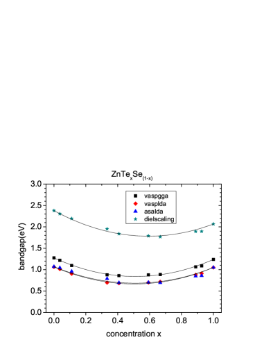
Figure 2: The bandgaps of ZnTe_xSe_1-x calculated with the LDA, the GGA, and Eq. (2) at various compositions $x$ . The squares and the diamonds indicate the GGA-VASP and the LDA-VASP results, respectively; the triangles and the stars represent the values of the LDA-TB-LMTO-ASA and of the DSA, respectively. The continuous lines are the results of the fitting. No spin-orbit coupling was considered.

Fig. 2 shows the bandgaps calculated with GGA-VASP and LDA-VASP, with the TB-LMTO-ASA in the LDA, and with the DSA defined by (2). The TB-LMTO-ASA results were considered with combined corrections [40]. The bandgaps calculated with GGA-VASP are larger than the results of LDA-VASP over entire range of concentrations. The bandgaps of the binary constituents calculated with LDA-VASP are both 1.06 eV. The LDA ASA gives a bandgap value of 1.07 eV for ZnSe and 1.05 eV for ZnTe. The ASA values are pretty close to the LMTO full potential values which are 1.05 eV and 1.03 eV, respectively [17]. Over the whole range of Te concentration $x$, the LDA-ASA results are in quite good agreement with the results obtained with PAW-VASP, which, in principle, is a full potential method with no shape approximation. Fig. 2 also shows the bandgaps calculated with the DSA, which exhibits much larger bandgaps than both the LDA and the GGA. The bandgaps of ZnSe and ZnTe calculated with the DSA are 2.38 eV and 2.07 eV, respectively, being comparable with the results of the GWA, which, in general, underestimates the bandgaps because it generates too much screening due to overestimation of $\chi^{0}$ [17].

As we expected, the bandgaps show a bowing, i.e., the bandgap deviates from linear interpolation with respect to composition $x$. The bowing parameter $b$ is 1.64 eV for the VASP-GGA and 1.57 eV for the VASP-LDA. The LDA of the TB-LMTO-ASA produces a bowing of 1.50 eV, while the DSA estimates the bowing parameter to 1.71 eV. The bowing parameters predicted with methods that go beyond the LDA are larger. The fact that the LDA does not reproduce the entire bowing of the bandgap is rooted not only in the LDA’s inability to predict the bandgap but also in the overbinding produced by the LDA. For ZnTe, ZnSe, and ZnTe_xSe_1-x the LDA overbinding pushes the cation d levels closer to the top of the valence band. Thus the $d$ levels will mix too much with the p states at the maximum of the valence band; therefore additional errors in estimating the band bowing occur. On the other hand it is known that the GWA moves these cation $d$ states in the right direction downwards [17].

Old measurements of the bandgap bowing parameters $b$ with and without spin-orbit interaction are presented in [44]. The authors estimated that the bandgap bowing is $b=1.266$ eV. They also estimated the spin-orbit splitting, which shows a concave bowing. Thus their estimated bandgap bowing without spin-orbit coupling is $b=1.07$ eV. Other measurements estimate a bowing parameter of 1.62 eV (at 5 K) and 1.51 eV (at 300 K) [45]. More recent experiments set the bowing of the bandgap between 1.25 eV and 1.5 eV at 300 K [4, 46] and the bowing of the spin-orbit splitting at -0.33 eV [4]. Other measurements at low temperature, namely at 13 K, indicate a bowing parameter around 2.21 eV [47].

Several general features can be outlined from all experimental data and our calculations. More recent experiments reveal larger band bowing coefficients than the older ones. The bowing is larger at low temperatures. There is also a bowing of the spin-orbit splitting but it is negative. The bandgap bowing calculated with spin-orbit coupling is larger than the bandgap bowing without spin-orbit coupling by one third of the bowing parameter modulus of the spin-orbit splitting. Overall, our results for bandgap bowing are in rather good agreement with recent experimental results.

4 Summary and Conclusions

To summarize, we have presented a computational scheme that realistically estimates the bandgaps and band bowing parameters with applicability to semiconductors and their alloys. The scheme uses the static polarization function $\chi^{0}$ to calculate the high-frequency dielectric constant $\varepsilon_{\infty}$ in the GF-TB-LMTO formalism. The corrections to the LDA bandgaps are made with a dielectric scaling approximation (DSA), which estimates the correction to the LDA bandgap as a universal constant divided by the high-frequency dielectric constant.

The approach inherits its speed from the fact that it works piecewisely to calculate $\chi^{0}$ via GF formalism and its efficiency from the TB-LMTO (the use of the muffin-tin orbitals and a minimal basis).

The limitations of the method were already discussed in [26]. The narrow-bandgap semiconductors are particularly difficult to describe with the DSA because the other corrections of the GWA to the the LDA bandgap become as important as the DSA. Also, often in these semiconductors there might appear a wrong ordering of the LDA levels around the bandgap with poor results in GWA too [17].

We applied the scheme to the ternary alloy ZnTe_xSe_1-x by calculating the bandgap and band bowing in a supercell with 54 atoms that mimics the alloying of ZnTe_xSe_1-x. The ternary alloy ZnTe_xSe_1-x exhibits large bandgap bowing. The bandgap bowing computed with the DSA is in good agreement with the experimental data. It was also shown that the bowing of the bandgap in ZnTe_xSe_1-x cannot be explained by the LDA alone due to inherent bowing shown also by the dielectric constant.

5 Acknowledgments

This work has been supported in part by the Romanian Ministry of Education and Research under the project “Ideas” No.120/2007. The work was also partially supported by the Natural Science and Engineering Research Council of Canada (NSERC) grant and was made possible by the computational resources of the Reseau Québecois de Calcul de Haute Performance (RQCHP).

References

- Shan et al. [1999] W. Shan, W. Walukiewicz, J. W. A. III, E. E. Haller, J. F. Geisz, D. J. Friedman, J. M. Olson, S. R. Kurz, Phys. Rev. Lett. 82 (1999) 1221.
- Alberi et al. [2007] K. Alberi, J. Wu, W. Walukiewicz, K. M. Yu, O. D. Dubon, S. P. Watkins, C. X. Wang, X. Liu, Y.-J. Cho, J. Furdyna, Phys. Rev. B 75 (2007) 045203.
- Walukiewicz et al. [2000] W. Walukiewicz, W. Shan, K. M. Yu, J. W. A. III, E. E. Haller, I. Miotkowski, M. J. Seong, H. Alawadhi, A. K. Ramdas, Phys. Rev. Lett. 85 (2000) 1552.
- Wu et al. [2003a] J. Wu, W. Walukiewicz, K. M. Yu, J. W. A. III, E. E. Haller, I. Miotkowski, A. K. Ramdas, C. H. Su, I. K. Sou, R. C. C. Perera, J. D. Denlinger, Phys. Rev. B 67 (2003a) 035207.
- Yu et al. [2003] K. M. Yu, W. Walukiewicz, J. Wu, W. Shan, J. W. Beeman, M. A. Scarpulla, O. D. Dubon, P. Becla, Phys. Rev. Lett. 91 (2003) 246403.
- Alberi et al. [2008] K. Alberi, J. Blacksberg, L. D. B. S. Nikzad, K. M. Yu, O. D. Dubon, W. Walukiewicz, Phys. Rev. B 77 (2008) 073202.
- Tit et al. [2009] N. Tit, I. M. Obaidat, H. Alawadhi, J. Phys.: Condens. Matter 21 (2009) 075802.
- Sandu and Kirk [2005] T. Sandu, W. P. Kirk, Phys. Rev. B 72 (2005) 073204.
- Kent and Zunger [2001] P. R. C. Kent, A. Zunger, Phys. Rev. B 64 (2001) 115208.
- Lindsay and O’Reilly [2004] A. Lindsay, E. P. O’Reilly, Phys. Rev. Lett. 93 (2004) 196402.
- Zunger et al. [1990] A. Zunger, S. W. Wei, L. G. Ferreira, J. E. Bernard, Phys. Rev. Lett. 65 (1990) 353.
- Kohn and Sham [1965] W. Kohn, L. J. Sham, Phys. Rev. 140 (1965) A1133.
- Hohenberg and Kohn [1964] P. Hohenberg, W. Kohn, Phys. Rev. 136 (1964) B864.
- Perdew et al. [1996] J. P. Perdew, K. Burke, M. Ernzerhof, Phys. Rev. Lett. 77 (1996) 3865.
- Hedin [1965] L. Hedin, Phys. Rev. 139 (1965) A796.
- Aryasetiawan and Gunnarsson [1998] F. Aryasetiawan, O. Gunnarsson, Rep. Prog. Phys. 61 (1998) 237.
- van Schilfgaarde et al. [2006] M. van Schilfgaarde, T. Kotani, S. V. Faleev, Phys. Rev. B 74 (2006) 245125.
- Hedin [1995] L. Hedin, Int. J. Quantum Chem. 56 (1995) 445.
- del Puerto et al. [2008] M. L. del Puerto, M. L. Tiago, J. R. Chelikowsky, Phys. Rev. B 77 (2008) 045404.
- Gygi and Baldereschi [1989] F. Gygi, A. Baldereschi, Phys. Rev. Lett. 62 (1989) 2160.
- Bechstedt et al. [1992] F. Bechstedt, R. D. Sole, G. Cappellini, L.Reining, Solid State Commun. 84 (1992) 765.
- Bylander and Kleinman [1990] D. M. Bylander, L. Kleinman, Phys. Rev. B 41 (1990) 7868.
- Seidl et al. [1996] A. Seidl, A. Gorling, P. Vogl, J. A. Majewski, M. Seidl, Phys. Rev. B 53 (1996) 3764.
- Furthmuller et al. [2002] J. Furthmuller, G. Cappellini, H. C. Weissker, F. Bechstedt, Phys. Rev. B 66 (2002) 045110.
- Lee and Wang [2006] B. Lee, L. W. Wang, Phys. Rev. B 73 (2006) 153309.
- Fiorentini and Baldereschi [1995] V. Fiorentini, A. Baldereschi, Phys. Rev. B 51 (1995) 17196.
- Kersch and Fischer [2008] A. Kersch, D. Fischer, J. Appl. Phys. 106 (2008) 014105.
- Gruning et al. [2006] M. Gruning, A. Marini, A. Rubio, Phys. Rev. B 74 (2006) 161103(R).
- Harrison [1985] W. A. Harrison, Phys. Rev. B 31 (1985) 2121.
- Tran and Blaha [2009] F. Tran, P. Blaha, Phys. Rev. Lett. 102 (2009) 226401.
- Kresse and Furthmüller [1996] G. Kresse, J. Furthmüller, Phys. Rev. B 54 (1996) 11169.
- Kresse and Joubert [1999] G. Kresse, D. Joubert, Phys. Rev. B 59 (1999) 1758.
- Andersen and Jepsen [1984] O. K. Andersen, O. Jepsen, Phys. Rev. Lett. 53 (1984) 2571.
- Andersen et al. [1986] O. K. Andersen, Z. Pawlowska, O. Jepsen, Phys. Rev. B 34 (1986) 5253.
- Turek et al. [1997] I. Turek, V. Drchal, J. Kudrnovsky, M. Sob, P. Weinberger, Electronic Structure of Disordered Alloy, Surfaces, and Interfaces, Kluwer Academic Publishers, Boston, MA, 1997.
- Glotzel et al. [1980] D. Glotzel, B. Segal, O. K. Andersen, Solid State Commun. 36 (1980) 403.
- Adler [1962] S. L. Adler, Phys. Rev. 126 (1962) 413.
- Wiser [1963] N. Wiser, Phys. Rev. 129 (1963) 62.
- Baroni and Resta [1986] S. Baroni, R. Resta, Phys. Rev. B 33 (1986) 7017.
- Skriver [1984] H. L. Skriver, The LMTO Method, Springer-Verlag, Berlin, 1984.
- Vegard [1921] L. Vegard, Z. Phys. 5 (1921) 17.
- Monkhorst and Pack [1976] H. J. Monkhorst, J. D. Pack, Phys. Rev. B 13 (1976) 5188.
- Kootstra et al. [2000] F. Kootstra, P. L. de Boeij, J. G. Snijders, Phys. Rev. B 62 (2000) 7071.
- Ebina et al. [1974] A. Ebina, Y. Sato, T. Takahashi, Phys.Rev. Lett 32 (1974) 1366.
- Brasil et al. [1991] M. S. J. P. Brasil, R. E. Nahory, F. S. Turco-Sandorf, H. L. Gilchrist, R. J. Martin, Appl. Phys. Lett. 58 (1991) 2509.
- Wu et al. [2003b] J. Wu, W. Walukiewicz, K. M. Yu, W. Shan, J. W. Ager, E. E. Haller, I. Miotkowski, A. K. Ramdas, C. H. Su, Phys. Rev. B 68 (2003b) 033206.
- Lin et al. [2008] Y. C. Lin, W. C. Chou, W. C. Fan, J. T. Ku, F. K. Ke, W. J. Wang, S. L. Yang, W. K. Chen, W. H. Chang, C. H. Chia, Appl. Phys.Lett. 93 (2008) 241909.