A Clipping Method to Mitigate the Impact of Catastrophic Photometric Redshift Errors on Weak Lensing Tomography

Abstract

We use the mock catalog of galaxies, constructed based on the COSMOS galaxy catalog including information on photometric redshifts (photo-$z$) and SED types of galaxies, in order to study how to define a galaxy subsample suitable for weak lensing tomography feasible with optical (and NIR) multi-band data. Since most of useful cosmological information arises from the sample variance limited regime for upcoming lensing surveys, a suitable subsample can be obtained by discarding a large fraction of galaxies that have less reliable photo-$z$ estimations. We develop a method to efficiently identify photo-$z$ outliers by monitoring the width of posterior likelihood function of redshift estimation for each galaxies. This clipping method may allow to obtain clean tomographic redshift bins (here three bins considered) that have almost no overlaps between different bins, by discarding more than $\sim 70\%$ galaxies of ill-defined photo-$z$’s corresponding to the number densities of remaining galaxies less than $\sim 20$ per square arcminutes for a Subaru-type deep survey. Restricting the ranges of magnitudes and redshifts and/or adding near infrared data help obtain a cleaner redshift binning. By using the Fisher information matrix formalism, we propagate photo-$z$ errors into biases in the dark energy equation of state parameter $w$. We found that, by discarding most of ill-defined photo-$z$ galaxies, the bias in $w$ can be reduced to the level comparable to the marginalized statistical error, however, the residual, small systematic bias remains due to asymmetric scatters around the relation between photometric and true redshifts. We also use the mock catalog to estimate the cumulative signal-to-noise ($S/N$) ratios for measuring the angular cross-correlations of galaxies between finner photo-$z$ bins, finding the higher $S/N$ values for photo-$z$ bins including photo-$z$ outliers.

1. Introduction

The bending of light by mass, gravitational lensing, causes images of distant galaxies to be distorted (e.g. Bartelmann & Schneider, 2001, for a thorough review). These sheared source galaxies are mostly too weakly distorted to measure the effect in individual galaxies, but requires surveys containing at least millions of galaxies to detect the signal in a statistical way (e.g. see Fu et al., 2008, for the latest measurement result). This cosmic shear is now recognized as one of the most promising probe that allows a direct reconstruction of the dark matter distribution as well as to constrain the properties of dark energy or to test the theory of gravity on cosmological scales (e.g. Hoekstra & Jain, 2008; Massey et al., 2010; Huterer, 2010, for recent reviews). In particular, by adding redshift information of source galaxies the lensing geometrical information as well as the redshift evolution of dark matter clustering can be inferred, thereby allowing to significantly improve its ability of constraining cosmology (e.g. Hu, 1999; Huterer, 2002; Takada & Jain, 2004).

To address questions about the nature of dark energy and/or the properties of gravity on cosmological scales, a number of ambitious wide-field optical and infrared imaging surveys have been proposed: the Panoramic Survey Telescope & Rapid Response System (Pan-STARRS), the Dark Energy Survey (DES), the Large Synoptic Sky Survey (LSST), the space-based Joint Dark Energy Mission (JDEM ), and the EUCLID. However, there are several sources of systematic errors inherent in weak lensing measurements, and understanding the systematic errors is currently the most important issue for achieving the full potential of planned lensing surveys (e.g. Huterer, 2010).

One of the most dangerous systematic errors is the uncertainty in estimating redshifts of source galaxies. Since it is practically infeasible to obtain spectroscopic redshifts for the huge number of imaging galaxies ($10^{8}$–$10^{9}$ galaxies for future surveys), redshifts of galaxies need to be estimated from multi-band photometry – the so-called photometric redshifts (hereafter photo-$z$). Both statistical errors and systematic biases in the relation between photometric and spectroscopic redshifts need to be well controlled (e.g. a sub-percent level for the bias for future surveys) in order not to have any serious biases in cosmological parameters comparable with the apparent statistical errors (Huterer et al., 2006; Ma et al., 2006). Understanding the properties of photo-$z$ errors is also important in exploring an optimal survey design given the goal of achieving the desired level cosmological constraints; depth vs number of filters vs area surveyed. Given these research backgrounds there are recent studies on photo-$z$ requirement studies based on real data (Abdalla et al., 2008; Lima et al., 2008; Cunha et al., 2009).

In this paper we would like to focus on an issue of how to identify and remove catastrophic redshift errors – the case that photometric redshift is grossly misestimated (also see Bernstein & Huterer, 2009, for the similar study). This can be done by monitoring the posterior likelihood function of photo-$z$ estimation for each galaxies. The important fact is that future surveys are planned to use the sample variance limited regime in cosmic shear information rather than the shot noise regime in order to constrain cosmology. Therefore one can discard a large fraction of galaxies whose photo-$z$ estimations are less reliable (Jain et al., 2007). Thus it would be worth addressing how to construct a galaxy subsample suitable for lensing experiments. Having such a subsample of galaxies with reliable photo-$z$ estimates may also relax requirements on a spectroscopic training set to calibrate the residual photo-$z$ errors. In this paper we will address these issues by using the mock catalog of photometric galaxies constructed based on the COSMOS photo-$z$ catalog (Ilbert et al., 2009) that provides the currently most reliable photo-$z$ catalog calibrated with 30 bands data and spectroscopic subsample.

This paper is organized as follow. In Section 2, we briefly overview the theory of weak lensing. In Section 3 we describe the details on how to make our simulated mock catalog of photometric galaxies based on the COSMOS data. In Section 4 we use the simulated catalog to assess the performance of photo-$z$ estimation assuming survey parameters on depth and filter set, which are closely chosen to resemble the Subaru Hyper Suprime-Cam(HSC) Survey. In Section 5 we show the main results: we use the simulated photo-$z$ catalog to implement hypothetical weak lensing experiment, paying particular attention to how to construct a galaxy subsample which is defined such that it has minimal impact of the photo-$z$ errors on cosmological parameters. Section 6 is devoted to summary and discussion. Unless explicitly stated we assume the concordance $\Lambda$CDM model consistent with the WMAP 5-year results (Komatsu et al., 2009).

2. Preliminaries

In this section we briefly review the basics of cosmic shear tomography. Throughout this paper we work in the context of a spatially flat cold dark matter model for structure formation.

2.1. Convergence Power Spectrum

Gravitational shear can be simply related to the lensing convergence: the weighted mass distribution integrated along the line of sight (e.g. see Bartelmann & Schneider, 2001, for a thorough review and references therein). Photometric redshift information on source galaxies allows us to subdivide galaxies into redshift bins, enabling more cosmological information to be extracted, which is referred to as lensing tomography (e.g. Hu, 1999; Huterer, 2002; Takada & Bridle, 2007). In the context of cosmological gravitational lensing, assuming the flat-sky approximation and the Limber’s approximation, the lensing power spectrum of the $i,j$-th tomographic bins can be expressed as

$$P^{\kappa}_{ij}(\ell)=\int_{0}^{\infty}dz\frac{W_{i}(z)W_{j}(z)}{\chi^{2}(z)H(z)}P_{\delta}\!\left(k=\frac{l}{\chi};z\right)$$ (1)

where $H(z)$ is the Hubble expansion rate, $\chi$ is the comoving angular diameter distance up to redshift $z$, and $P_{\delta}(k,z)$ is the three-dimensional matter power spectrum at scale $k$ and at redshift $z$. The lensing weight function $W_{(i)}(\chi)$ in the $i$-th tomographic redshift bin, defined to lie between the redshifts $z_{i}$ and $z_{i+1}$, is given by

$$W_{i}(z)=\frac{3}{2}\Omega_{\rm m0}H^{2}_{0}g_{i}(z)(1+z),$$ (2)

and

$$g_{i}(z) = \left\{\begin{array}[]{ll}{\displaystyle\chi(z)\int_{{\rm max}(z,z_{i})}^{z_{i+1}}\!\!dz^{\prime}\frac{n(z^{\prime})}{\bar{n}_{i}}\left[1-\frac{\chi(z)}{\chi(z^{\prime})}\right]},&z<z_{i+1}\\ 0,&z>z_{i+1}\end{array}\right.$$ (4)

where $n(z)$ is the redshift distribution of galaxies, and $\bar{n}_{i}$ is the average number density of galaxies residing in the $i$-th tomographic bin (or the redshift range $z=[z_{i},z_{i+1}]$): $\bar{n}_{i}=\int_{z_{i}}^{z_{i+1}}dz^{\prime}n(z^{\prime})$.

In practice the power spectrum measured from a galaxy survey has shot noise contamination arising from the finite sampling of galaxy images. Hence the measured power spectrum becomes

$$C_{ij}^{\kappa}(l)=P^{\kappa}_{ij}(l)+\frac{\sigma_{\epsilon}^{2}}{\bar{n}_{i}}\delta^{K}_{ij},$$ (5)

where $\sigma_{\epsilon}$ is the rms intrinsic ellipticities per component and $\delta_{ij}^{K}$ is the Kronecker delta symbols; $\delta^{K}_{ij}=1$ when $i=j$, otherwise $\delta^{K}_{ij}=0$.

Note that the distribution $n(z)$ appearing in Eq. (2) denotes the underlying true redshift distribution of galaxies used in lensing analysis. However, the distribution needs to be inferred from photo-$z$ information of individual galaxies available from multi-color imaging data sets. This generally causes biases in the lensing power spectrum in the presence of photo-$z$ errors. As long as tomographic redshift bins are broad enough, $O(10^{7})$ galaxies are available in each bin for a Subaru-type survey with $\sim$1000 degree² sky coverage. Therefore the statistical errors of photo-$z$ are not problematic: the lensing power spectrum is primarily sensitive to the mean redshift of source galaxies. Instead, a precise knowledge of the mean redshift in each tomographic bin is required not to have any significant biases in best-fit parameters compared to the statistical errors, as studied in Huterer et al. (2006).

To assess the required photo-$z$ accuracies for lensing tomography, an important fact we should keep in mind is the lensing measurement for planned wide-field surveys is not shot noise limited. Hence a significant fraction of galaxies with ill-defined photo-$z$’s can be discarded, without severely degrading parameter accuracies (Jain et al., 2007). With these considerations in mind we will in the following address how to define an adequate subsample of galaxies for a given multi-color data set.

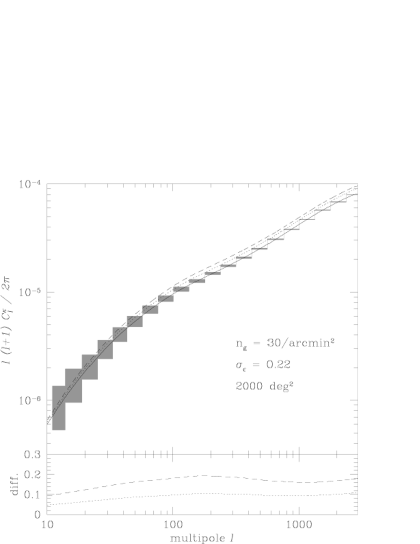
Figure 1.— The solid curve shows the lensing shear power spectrum assuming the concordance $\Lambda$CDM model and the galaxy redshift distribution with mean redshift $\langle z\rangle=1.13$ (see text for the details). The dashed curve shows the resulting spectrum when the mean redshift is shifted by $5\%$, while the dotted curve shows the spectrum when the dark energy equation of state parameter is changed to $w=-1.2$. The shaded boxes around the fiducial power spectrum show the expected $1\sigma$ error at each multipole bins assuming $\Omega_{\rm S}=2000$deg², $\bar{n}_{g}=30$ arcmin^-2, and $\sigma_{\epsilon}=0.22$ for survey area, the average number density of galaxies and the rms intrinsic ellipticities, respectively. The bottom panel shows the relative differences of power spectra with respect to the fiducial spectrum.

Figure 1 gives a quick summary of the impact of redshift uncertainty on the lensing power spectrum for no tomography case, i.e. a single redshift bin. Here for simplicity we assumed the redshift distribution given by the analytical form, $n(z)\propto z^{2}\exp[-(z/z_{0})^{2}]$ with $z_{0}=1$, corresponding to the mean redshift $\langle z\rangle=2z_{0}/\sqrt{\pi}\simeq 1.12$. (Note that the following results are all computed using simulated galaxy catalogs that have different redshift distributions). The plot shows that a $5\%$ change in the mean redshift causes a $10\%$-level change in the power spectrum amplitude, and the amount of the change varies with multipoles due to the projection of the nonlinear matter power spectrum. This change can be compared with the effect of dark energy equation of state and the statistical errors at each multipole bin expected for the power spectrum measurement. Clearly such a bias in the mean redshift is problematic for planned surveys.

3. A Simulation of Photometric Galaxy Catalog

To assess the impact of photo-$z$ errors on cosmic shear tomography, we take the following procedure. First we simulate a mock catalog of galaxies that contain information on true redshifts, magnitudes in each filters and spectral energy distribution (SED) for survey parameters we consider. Then we estimate photometric redshifts (hereafter often photo-$z$) for each simulated galaxies from its colors, yielding the photo-$z$ catalogs.

A quick summary of the procedures used in making the mock photometric catalog is as follows:

1. Based on the results of COSMOS photo-$z$ catalog (Ilbert et al., 2009), we first model the redshift distribution of galaxies as a function of the $i$-band magnitudes down to $i=25.8$ (see § 3.1).

2. Use the synthetic galaxy spectral model, GISSEL98, to generate a set of SED templates for each type of galaxy, where the age and star formation history are randomly varied (see § 3.2).

3. Use the HyperZ code to generate a mock photometric catalog of galaxies in which the spectral energy distribution and redshift are assigned to each galaxy. In doing this the catalog is made by imposing the conditions that the catalog satisfy the redshift-magnitude relation as well as reproduce an appropriate mixture of galaxy SED types which is consistent with the COSMOS galaxy population (see § 3.3).

4. For a given set of filters, compute apparent magnitudes in each filter for each simulated galaxy by taking into account the filter transmission curve and the redshifted spectrum (see § 3.4). The statistical magnitude errors are also added to the magnitude of each filter (see § 3.5).

To make a realistic simulated catalog, we assume survey parameters (depth, filter transmission curves, and so on) that are chosen to well resemble the planned HSC survey. We also consider the external imaging data sets of $u$-band and/or NIR to study how combining the different colors improves photo-$z$ accuracies.

In this paper we use the mock galaxy catalog containing about $10^{5}$ galaxies in the range $20<i<25.8$.

In the following subsections we will describe the details of each procedure above, and a reader who is more interested in the results can skip these subsections and go to § 4.

3.1. Magnitude-Redshift Relation

Figure 2.— The redshift distribution of our simulated galaxies (containing about $10^{5}$ galaxies) as a function of the $i$-band magnitude ranges as indicated by the labels. Note that the mock catalog is constructed so as to reproduce the redshift distribution found in the COSMOS galaxies with $i<25$. The galaxies with $25<i<25.8$ are simulated by extrapolating the COSMOS results down to the fainter magnitudes (see text for the details).

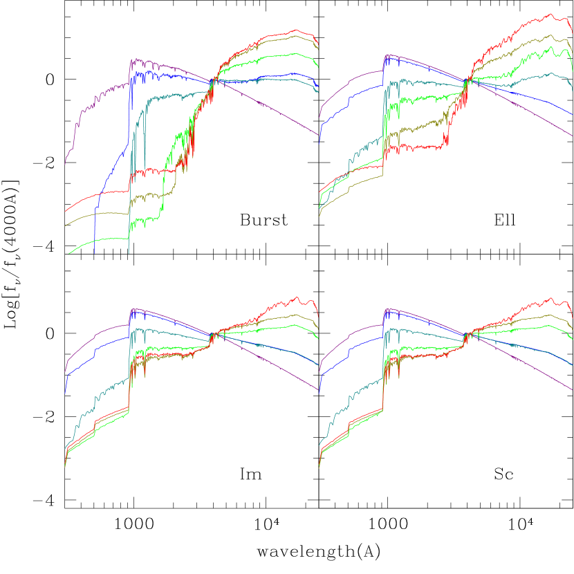
Figure 3.— Plotted are synthetic galaxy spectra, $f_{\nu}=\lambda^{2}f_{\lambda}$ normalized at $\lambda=4000$Å. For each panel, from top to bottom at $10000$Å, galaxy ages are 10Gyr, 5Gyr, 1Gyr, 100Myr, 10Myr and 1Myr, respectively. From the top-left to bottom-right panels, the galaxy SED types are star-burst (SB), elliptical (Ell), irregular (Im), and spiral (Sc), respectively.

To make a mock catalog we need to properly take into account the redshift distribution of galaxies, which varies with the range of magnitudes considered. For example, fainter galaxies are preferentially at higher redshifts. This is the so-called magnitude-redshift relation. We use the magnitude-redshift relation estimated from the COSMOS catalog of galaxies selected by the Subaru $i$-band magnitudes (Ilbert et al., 2009). The COSMOS catalog provides currently the most accurate photometric redshifts because the photo-$z$ are estimated from 30 broad, intermediate, and narrow bands covering from UV, optical to mid infrared. Also the photo-$z$ estimates are calibrated by the spectroscopic sub-sample. Ilbert et al. (2009) studied subsamples of photo-$z$ galaxies for different limiting magnitudes and showed that the resulting redshift distributions are well fitted by the polynomial form:

$$n(z)=A\frac{z^{ab}+z^{a}}{z^{b}+c},$$ (6)

where $A$, $a,b$ and $c$ are the fitting parameters. The best-fit parameters for different magnitudes in the range $i=[22,25]$ are given in Table 2 in Ilbert et al. (2009). The COSMOS data is deep enough in the $i$-band, and safely considered as a magnitude limit sample for $i<25$. The COSMOS catalog also includes information on the angular number counts of galaxies for a given magnitude range as well as on the estimated galaxy SED type for each galaxy. To model a hypothetically deeper survey we are interested in, we extrapolate the fitting parameters to obtain the redshift distribution for fainter galaxies down to $i=25.8$.

We thus generate a mock $i$-band photometric catalog of galaxies such that the resulting catalog satisfies the magnitude and redshift relation for different ranges of $i$-band magnitudes. Figure 2 shows the magnitude-redshift distributions for the simulated catalog containing about $10^{5}$ galaxies.

3.2. Synthetic Spectral Models

For a given simulated galaxy labeled with some $i$-band magnitude and redshift $z$, we need to model the spectral energy distribution from which the apparent magnitudes can be computed for a given set of filters. We use the publicly available library GISSEL98 (Bruzual & Charlot, 1993, 2003; Bolzonella et al., 2000) to model the synthetic galaxy spectrum. The galaxy SEDs are generated to represent from early- to late-type SEDs (elliptical, S0, Sa, Sb, Sc, Sd, Im and starburst). To model these populations – composite stellar populations (CSPs) – the single stellar population (SSP) is convolved with a model star formation history:

$$f_{\rm CSP}(t)=\int_{0}^{t}\psi(t-\tau)f_{\rm SSP}(\tau)d\tau.$$ (7)

Note that the SSP is modeled in Bruzual & Charlot (1993), with the initial stellar mass function given in Miller & Scalo (1979). The function $\psi(t)$ is the star formation rate at galaxy age $t$. We assumed $\psi(t)\propto\exp(-t/\tau)$ with $\tau=1,2,3,5,15,30$ Gyr for elliptical, S0, Sa, Sb, Sc, and Sd galaxies, respectively. For a starburst galaxy, the star formation is instantaneously occurred, while $\psi={\rm constant}$ for an irregular (Im) galaxy. The metalicity is self-consistently evolved with galaxy age, and we checked that different models of metalicity little change the photo-$z$ estimates (also see Bolzonella et al., 2000). We randomly chosen the age of each simulated galaxy from 221 different ages in the range of $t=[0,20]$ Gyr, where the age interval is done according to GISSEL98.

Figure 3 demonstrates simulated SEDs for starburst, elliptical, irregular, and spiral galaxies for 6 different ages. The dust extinction is modeled following Calzetti et al. (2000) with $A_{V}$ in the range [0,2.0].

3.3. Mock Galaxy Catalog

To make a mock galaxy catalog containing various galaxy populations, we used the publicly available code HyperZ. In doing this we need to account for an appropriate mixture of different galaxy SED types. We employed the composition (SB, E, S, Im)=(0.52, 0.035, 0.40, 0.045) over all the redshift range, which is chosen so as to match the composition of best-fit galaxy SED types found from the COSMOS catalog with $i<25$ . For this purpose the command make_catalog in HyperZ was slightly modified in such a way that the resulting catalog satisfies the magnitude-redshift relations for each magnitude range in § 3.1 and the assumed composition of galaxy SED types, because the original make_catalog generates a catalog that redshift, reference magnitude, age, galaxy SED type and the amount of dust extinction are randomly assigned to each galaxy.

3.4. Photometric Magnitudes

Once the spectral energy distribution is specified for each simulated galaxy at redshift $z$, it is straightforward to compute the apparent magnitudes for a given set of filters taking into account the redshifted spectrum at observed wavelengths. The photo-$z$ estimate is sensitive to the details of observational parameters: the wavelength coverage, the transmission curve of a given filter, the exposure time, the limiting magnitude, and so on. We consider the parameters that match those of the planned Subaru HSC survey: our default filter set is $g^{\prime}r^{\prime}i^{\prime}z^{\prime}y^{\prime}$ (hereafter the prime superscripts are sometimes omitted), and the $5\sigma$ limiting magnitudes ($2^{\prime\prime}$ aperture) are set to $g=26.5$, $r=26.4$, $i=25.8$, $z=24.9$, and $y=23.7$, respectively, assuming the exposure time of 15 minutes for each pass-band, 3 days from new moon, and 1.2 airmass at the Subaru Telescope site.

We also study how adding other bands, $u$-band data and NIR data, into the optical data above can improve photo-$z$ accuracies. Having a wider wavelength coverage helps break degeneracies in photo-$z$ estimates, more exactly helps discriminate the Lyman break and 4000 angstrom break, from the multi-color data. We here consider the $u$-band data that can be delivered from CFHT, and also the $J,H,K_{s}$(hereafter $K$) bands of planed VIKING (VISTA Kilo-Degree Infrared Galaxy) survey. The 5$\sigma$ limiting magnitudes are $u=25.0$, $J=22.1$, $H=21.5$ and $K=21.2$, respectively. The set of filters and the depths we consider in this paper are summarized in Table 1.

Detailed study for the optimal filter parameters, for example, the number of filters, filter resolution, in terms of minimizing the outlier fraction or photo-z scatters are found in Jouvel et al. (2010).

Table 1Filters and limiting magnitudes ($5\sigma$)

Filter	Survey	$\lambda_{c}$(Å)	FWHM(Å)	ABmag	Texp(sec)
$u*$	CFHTLS	3752	740	25.0	900
$g^{\prime}$	HSC	4814	1120	26.5	900
$r^{\prime}$	HSC	6279	1370	26.4	900
$i^{\prime}$	HSC	7687	1500	25.8	900
$z^{\prime}$	HSC	9143	1330	24.9	900
$y^{\prime}$	HSC	9923	490	23.7	900
$J$	VIKING	12578	1713	22.1	420
$H$	VIKING	16581	2828	21.5	420
$K$	VIKING	21790	2828	21.2	420

3.5. Magnitude Errors

Finally we include statistical errors in the apparent magnitudes. Assuming the sky noise limit, we simply model this magnitude error as Gaussian fluctuations with width given by

$$\Delta m\simeq 2.5\log\left(1+\frac{1}{SN}\right),$$ (8)

where $SN$ is the signal-to-noise ratio for a given galaxy; $SN$ is computed once its apparent magnitude and the depth in the filter are given. The magnitude error is computed as follows. First, the sky noise is added to the observed flux of a galaxy, causing a deviation from the true flux as $f^{\rm obs}=f_{0}+\Delta f=f_{0}(1+1/SN)$. Then the magnitude error above is computed as $\Delta m=-2.5\log(1+1/SN)$ because $m_{0}+\Delta m=-2.5\log f_{0}(1+1/SN)+{\rm constant}$. Exactly speaking, even for a Gaussian sky noise, the magnitude error does not obey a Gaussian distribution due to the log-mapping. However, the Gaussian approximation on $\Delta m$ holds for galaxies with sufficiently high $SN$ values, which we will assume for the following results.

Note that a galaxy, which has its apparent magnitude near the limiting magnitude, may be excluded from or included in the sample in the presence of the magnitude error. While our simulated galaxies are all $i$-band selected, some galaxies may have apparent magnitudes below the detection limit in other pass-bands. We use such an upper limit on the flux in the photo-$z$ estimate, which improves the photo-$z$’s to some extent. In doing this the flux for such an undetected galaxy in a given filter is set to the magnitude corresponding to the halved limiting flux $f_{\rm lim}/2$. Also we note that the systematic offset of photometry may cause an additional uncertainty on magnitude measurement, which in this paper is ignored. Such a zero-point magnitude offset can be, for example, calibrated by using a spectroscopic redshift subsample (Ilbert et al., 2009).

According to the procedures described above we made a mock photometric catalog containing about $10^{5}$ galaxies down to the magnitude $i=25.8$. Although we tried to make a realistic mock catalog based on the COSMOS catalog, some of our treatments may be still oversimplified: for example, we assumed a single stellar population for galaxy SEDs. The simplified assumptions may make our results somewhat optimistic. A more accurate way to overcome these obstacles is using the real data including spectra for a representative subsample of imaging galaxies. However, such a spectroscopic data especially for faint galaxies of interest is still limited, and this is our future work.

4. Method: Photometric Redshift and Parameter Bias

Now we use the mock photometric catalog of $i$-band selected galaxies to assess the performance of photo-$z$ estimates in the context of weak lensing tomography experiment.

4.1. Photometric Redshift Estimation

By combining multi-passband magnitudes of a given imaging galaxy, its redshift can be estimated without spectroscopic observation – the so-called photo-$z$. There are various techniques that have been developed: the template fitting method (Sawicki et al., 1997; Bolzonella et al., 2000), the template method combined with prior information (magnitude prior and so on) (Benítez, 2000; Mobasher et al., 2004), the method including a self-calibration based on a training spectroscopic set (Collister & Lahav, 2004, and see references therein).

In this paper we use the publicly available code, Le Phare , which is a template fitting method. The photo-$z$ for each galaxy is estimated based on the $\chi^{2}$ fitting:

$$\chi^{2}=\sum_{i}^{N_{f}}\frac{\left[f_{i}^{\rm obs}-\alpha f(T,z,E)\right]^{2}}{\sigma_{i}^{2}},$$ (9)

where $f_{i}^{\rm obs}$ is the observed flux in the $i$-th filter, $f(T,z,E)$ is the model flux which is given as a function of galaxy SED type ($T$), redshift ($z$) and the amount of dust extinction ($E$), and $\sigma_{i}$ is the magnitude error. Note that galaxy SED type is modeled according to the method described in § 3.2. The summation runs over the number of filters considered ($N_{f}$). The extra factor parameter $\alpha$, which is the same in all the filters, is introduced in Eq. (9) because the photo-$z$ is estimated only from colors, the relative amplitudes of fluxes in different filters, not from the absolute fluxes. Therefore there are ($N_{f}$-1) constraints given the data of $N_{f}$ filters. The best-fit redshift parameter, i.e. the best-fit photo-$z$, is obtained by minimizing the $\chi^{2}$ value with varying other model parameters.

If the location of spectral features such as Lyman break and 4000Å  break is captured given the wavelength coverage of observed filters and the magnitude depths taken, the redshift is robustly estimated. On the other hand, a misidentification of the spectral features causes a degeneracy in redshift estimation, often yielding multiple solutions at low and high redshifts. Hence the photo-$z$ method based on broad band photometry generally yields a large fraction of outliers, where the best-fit photo-$z$ can be far from the true redshift. To quantify the photo-$z$ accuracy for each galaxy we will use the following two quantities: (1) the goodness-of-fit parameter for the template fitting, and (2) the width of likelihood function of redshift estimation.

The goodness-of-fit for the template fitting of a given galaxy may be defined as

$$\chi^{2}_{\nu}\equiv\frac{\chi^{2}_{\rm min}(z_{\rm bf})}{N_{f}-1},$$ (10)

where $\chi^{2}_{\rm min}$ is the minimum $\chi^{2}$ value for the best-fit model and redshift, $z_{\rm bf}$ is the best-fit redshift and $N_{f}-1$ is the number of colors available. Note that the quantity above, $\chi^{2}_{\nu}$, is not the same as the reduced $\chi^{2}$, which is defined as the number of constraints minus the number of model parameters. The number of model parameters are equal for all the galaxies, so $\chi^{2}_{\nu}$ gives a measure of the goodness-of-fit.

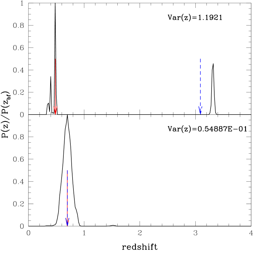
Figure 4.— Examples of the photo-$z$ fitting for two simulated galaxies. The upper panel shows an example of the photo-$z$ outlier, i.e. ill-defined photo-$z$ estimate, while the lower panel shows an example of the reliable photo-$z$ estimate. In each panel, the solid curve shows the likelihood function of redshift parameter, $p(z)\propto\exp[-\chi^{2}/2]$, and the solid (red) and dashed (blue) arrows denote the best-fit redshift and the true redshift, respectively. The width of the likelihood is quantified by ${\rm Var}(z)$, defined by Eq. (11), and the value for each simulated galaxy is denoted in the upper-right corner of each panel.

We also use the width of likelihood function of redshift estimation for each galaxy defined as

$${\rm Var}(z)\equiv\int_{0}^{\infty}\!dz~{}(z-z_{\rm bf})^{2}p(z)\frac{1}{(1+z_{\rm bf})},$$ (11)

where $p(z)$ is the likelihood function given as $p(z)\propto\exp[-\chi^{2}(z)/2]$, which is normalized so as to satisfy $\int\!dz~{}p(z)=1$. We compute the likelihood function $p(z)$ by fixing other model parameters to their best-fit values. The normalization factor $(1+z_{\rm bf})$ is introduced based on the fact that the photo-$z$ accuracy scales with $(1+z)$. Compared to $\sigma(z)$, the local standard deviation of photo-$z$ estimation, which is obtained from $\Delta\chi^{2}\leq 1$, the quantity ${\rm Var}(z)$ is sensitive to the outlier probability with $|z-z_{\rm bf}|\gg 1$ due to the weight $(z-z_{\rm bf})^{2}$. Hence for galaxies whose likelihood function has multiple peaks, i.e. multiple redshift solutions, the quantity ${\rm Var}(z)$ tends to be larger. The similar quantities to ${\rm Var}(z)$ are also used in the previous works (Mobasher et al., 2004; Wolf, 2009), where the primary purpose is to improve the photo-$z$ performance for a majority of galaxies. In this paper we use the figure-of-merit quantity ${\rm Var}(z)$ mainly for identifying photo-$z$ outliers.

Note that we will in the following results use $z_{\rm bf}$ to construct the redshift distribution of galaxies. An alternative method, which may be less sensitive to photo-$z$ outliers, is summing the photo-$z$ posterior likelihood function $p(z)$ over all the sampled galaxies to obtain the overall redshift distribution (Wittman, 2009; Cunha et al., 2009). Calibrating the mean redshift distribution is another important issue to be carefully studied (Ma & Bernstein, 2008; Bordoloi et al., 2009), but is beyond the scope of this paper.

Figure 4 demonstrates examples of the photo-$z$ fitting for two simulated galaxies. It can be found that a galaxy which has the ill-defined photo-$z$ estimate, i.e. the wider likelihood function of redshift estimation, tends to have a larger value of ${\rm Var}(z)$. In particular, even if the likelihood function locally has a narrow peak around the best-fit redshift, therefore even if the photo-$z$ error looks apparently small, the value ${\rm Var}(z)$ becomes larger if the likelihood has multiple peaks (i.e. the case of multiple redshift solutions), as demonstrated in the upper panel. On the other hand a galaxy with reliable photo-$z$ estimate has a small value of ${\rm Var}(z)$.

While the quantity ${\rm Var}(z)$ is rather empirically defined as an indicator of photo-$z$ outliers, Figure 5 gives a quantitative study of how ${\rm Var}(z)$ can characterize the photo-$z$ likelihood function. The figure shows the distributions of simulated galaxies in the ${\rm Var}(z)$–$\Delta z$ plane, where $\Delta z$ is the difference between true and photometric redshifts defined as $\Delta z\equiv(z_{\rm bf}-z_{\rm true})/(1+z_{\rm true})$ for each galaxy. According to the properties of their photo-$z$ likelihood functions, we divide galaxies into two subsamples: one (black-thick line) is defined from galaxies (about 25% fraction of all the galaxies) that have a single peak therefore a reliable photo-$z$ estimate, while the other (gray-thin line) is from galaxies of multiple peaks, respectively. Note that the second and higher-order peaks are defined from local maxima of the likelihood that have heights higher than 10% of the first peak height. One can find from the figure that the quantity ${\rm Var}(z)$ nicely separate galaxies that tend to have have greater photo-$z$ biases and multiple solutions of photo-$z$’s, i.e. degenerate photo-$z$ estimate; most of galaxies having ${\rm Var(z)}\lower 2.15277pt\hbox{$\;\buildrel>\over{\sim}\;$}0.1$ have multiple peaks.

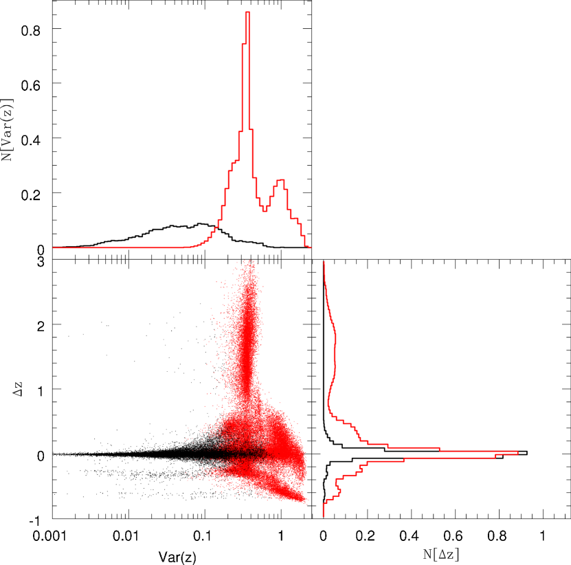
Figure 5.— The probability distributions of simulated galaxies in parameter space of ${\rm Var}(z)$ and $\Delta z$, where ${\rm Var}(z)$ is defined in terms of the photo-$z$ likelihood by Eq. (11) and $\Delta z$ denote the bias between photometric and true redshifts, $\Delta z\equiv(z_{\rm bf}-z_{\rm true})/(1+z_{\rm true})$. In each panel, black-thick dots or lines show galaxies whose photo-$z$ likelihood function has a single peak, while gray-thin dots or lines show galaxies that multiple peaks in their likelihood. It is clear that galaxies, which have greater photo-$z$ biases and have multiple photo-$z$ solutions in their likelihood, tend to have greater values of ${\rm Var}(z)$.

4.2. Fisher matrix formalism

We will use the Fisher matrix formalism to estimate accuracies of estimating parameters given the lensing power spectrum. The Fisher matrix is given by

$$F_{\alpha\beta}=\sum_{\ell=\ell_{\rm min}}^{\ell_{\rm max}}\sum_{i,j,m,n}\frac{\partial C^{\kappa}_{ij}(\ell)}{\partial p_{\alpha}}{\bf C}^{-1}\!\!\left[C^{\kappa}_{ij}(\ell),C^{\kappa}_{mn}(\ell)\right]\frac{\partial C^{\kappa}_{mn}(\ell)}{\partial p_{\beta}},$$ (12)

where $p_{\alpha}$ denotes a set of cosmological parameters, the matrix ${\bf C}$ denotes the covariance matrix, and ${\bf C}^{-1}$ denotes the inverse matrix. In this paper we simply use the covariance matrix given by the first term in Eq. (9) in Takada & Jain (2009) assuming the Gaussian errors on power spectrum measurements. The Gaussian error assumption is adequate for our purpose because the impact of non-Gaussian errors on parameter estimation is not significant as long as a multi-parameter fitting is considered as shown in Takada & Jain (2009). The marginalized $1\sigma$ error on the $\alpha$-th parameter $p_{\alpha}$ is given by $\sigma^{2}(p_{\alpha})=({\bf F}^{-1})_{\alpha\alpha}$, where ${\bf F}^{-1}$ is the inverse of the Fisher matrix. Throughout this paper we set $l_{\rm min}=5$ and $l_{\rm max}=3000$ as for the minimum and maximum multipoles in the summation above. Note that all the parameter forecasts shown below are for the lensing tomography combined with the expected Planck information, which is obtained simply by adding the two Fisher matrices of lensing and CMB: ${\boldsymbol{F}}_{\rm WL+CMB}={\boldsymbol{F}}_{\rm WL}+{\boldsymbol{F}}_{\rm CMB}$.

As explained around Eq. (1), the lensing power spectrum is sensitive to the underlying true redshift distribution of galaxies, $n(z)$. For a multi-color imaging survey, however, the distribution $n(z)$ needs to be estimated from the available photo-$z$ information. In this procedure the photo-$z$ errors affect weak lensing experiments. Most dangerous effect is a systematic bias in parameter estimations: if the inferred redshift distribution has a bias in the mean redshift compared to the true one, the redshift bias may cause significant biases in cosmological parameters. In order to quantify the biases in cosmological parameters caused by photo-$z$ errors, we use the following method based on the Fisher matrix formalism in Huterer & Takada (2005) (also see Appendix B of Joachimi & Schneider, 2009, for the detailed derivation):

$$\delta p_{\alpha} = \sum_{\beta}[{\boldsymbol{F}}_{\rm WL+CMB}^{-1}]_{\alpha\beta}\sum_{\ell}\sum_{i,j,m,n}\frac{\partial C^{\kappa}_{ij}(\ell)}{\partial p_{\beta}}$$

$$\times{\bf C}^{-1}[C^{\kappa}_{ij}(\ell),C^{\kappa}_{mn}(\ell^{\prime})]\left[C^{\kappa}_{mn}(\ell^{\prime})-C^{\kappa,{\rm photo-z}}_{mn}(\ell^{\prime})\right],$$

where ${\boldsymbol{F}}^{-1}_{\rm WL+CMB}$ is the inverse of the Fisher matrix, and $\delta p_{\alpha}$ denotes a bias in the $\alpha$-th parameter, the difference between the best-fit and true values. In the equation above, the spectrum $C_{mn}^{\kappa}(l)$ is the underlying true power spectrum, while $C^{\kappa,{\rm photo-z}}_{mn}(l)$ is the spectrum estimated from the redshift distribution inferred based on the photo-$z$ information. In the presence of the photo-$z$ errors, generally $C^{\kappa}_{ij}\neq C^{\kappa,{\rm photo-z}}_{ij}$, thereby causing a bias in parameter estimation. We can compute both spectra, $C^{\kappa}$ and $C^{\kappa,{\rm photo-z}}$ from a simulated galaxy catalog for a hypothetical lensing survey. Note that in Eq. (LABEL:eq:bias_theta_red), for simplicity, we have not considered any other nuisance parameters that model other systematic effects such as the shape measurement errors (e.g. Huterer et al., 2006) and the inability to make precise model predictions arising from nonlinear clustering and baryonic physics (Huterer & Takada, 2005; Rudd et al., 2008; Zentner et al., 2008).

To compute the parameter forecasts we need to specify a fiducial cosmological model and survey parameters. Our fiducial cosmological model is based on the WMAP 5-year results (Komatsu et al., 2009): the density parameters for dark energy, CDM and baryon are $\Omega_{\rm de}(=0.74)$, $\Omega_{\rm cdm}h^{2}(=0.1078)$, and $\Omega_{\rm b}h^{2}(=0.0196)$ (note that we assume a flat universe); the primordial power spectrum parameters are the spectral tilt, $n_{s}(=1)$, and the normalization parameter of primordial curvature perturbations, $A_{s}\equiv\delta_{\zeta}^{2}(=2.3\times 10^{-9})$ (the values in the parentheses denote the fiducial model); the dark energy equation of state parameter $w_{0}(=-1)$. We used the publicly available code CAMB developed in Lewis & Challinor (2006) (also see Seljak & Zaldarriaga, 1996) to compute the transfer function, and use the fitting formula in Smith et al. (2003) to compute the nonlinear mass power spectrum from which the lensing power spectrum is computed over the relevant range of angular scales.

Our fiducial survey roughly resembles the planned Subaru Hyper-Suprime Cam Survey (Miyazaki et al., 2006). We adopt the set of filters ($grizy$) and the depths in each filter as given in § 3. We will also study how the results change when the hypothetical Subaru survey is combined with other surveys that deliver the $u$-band data or/and the NIR data, which especially help improve the photo-$z$ accuracies. The survey area is throughout assumed to be $\Omega_{\rm s}=2000~{}$deg². The redshift distribution of galaxies is computed for an assumed subsample of galaxies based on the photo-$z$ information.

4.3. Object selection and clipping of photo-$z$ outliers

We may be able to construct a suitable subsample of galaxies in a sense that the impact of photo-$z$ errors are minimized in order not to have more than 100% biases in cosmological parameters compared to the statistical errors. Hence a selection of adequate galaxies is important for weak lensing: for example, this may be attained by discarding galaxies with ill-defined photo-$z$’s. However, the important fact we should keep in mind is that, with discarding more galaxies, the statistical accuracy of parameter estimation is degraded due to the increased shot noise contamination in the power spectrum measurement. Thus there would be a trade-off point in defining a suitable galaxy subsample in terms of the parameter bias versus the statistical error for a given survey.

We throughout this paper work on $i$-band selected galaxies assuming that the $i$-band data is used for the lensing shape measurement as often done in the previous lensing works. For our simulated galaxies, given the limiting magnitude $i=25.8$ at $5\sigma$ significance, a sufficiently number of photometric galaxies are available: the number density for total galaxies is 80 per square arcminutes. However, all the galaxies are not usable of lensing measurements. First, in order to obtain a reliable shape measurement, galaxies used in the lensing analysis need to be well resolved, requiring the galaxies to have sufficient signal-to-noise ratios (say more than $10\sigma$). Secondly, galaxies with ill-defined photo-$z$ estimates are not useful because including such galaxies may cause a significant bias in parameter estimation.

With the considerations above in mind, we will consider the following object selections or their combinations to make parameter forecasts.

• The restrictive range of $i$-band magnitudes: $22.5\leq i\leq 25$. The range is a typical one used in the weak lensing analysis (e.g. Okabe et al., 2009). The faint-end magnitude cut may be imposed such that the selected galaxies have sufficiently high signal-to-noise ratios: $i=25$ corresponds to $S/N\simeq 10$ in our simulations. The bright-end magnitude cut is not important, but usually imposed in practice to avoid galaxies with saturated pixels.

• The photo-$z$ selection. We select only galaxies that have reasonably good photo-$z$ estimates by imposing a threshold on the goodness-of-fit of photo-$z$ estimation, $\chi^{2}_{\nu}\leq 2$ (see Eq. [10]). The clipping threshold $\chi^{2}_{\nu}=2$ is not a unique choice. Rather we selected the value, as one working example.

• The restrictive range of photo-$z$’s: $0.2\leq z_{\rm bf}\leq 1.5$. The spectral features of galaxies in this range of redshifts can be relatively well captured by the wavelength coverage of optical filters. The lower redshift cut is introduced, because there is a strong degeneracy between galaxies at such low redshifts $z\lower 2.15277pt\hbox{$\;\buildrel<\over{\sim}\;$}0.2$ and those at higher redshifts, especially in a case that the $u$-band data is not available or shallower than optical data as considered in this paper.

• Clipping of photo-$z$ outliers. By discarding galaxies with ${\rm Var}(z)$ (see Eq. [11]) greater than a given threshold, which turn out to be mostly photo-$z$ outliers, we define a subsample from the remaining galaxies that have relatively reliable photo-$z$’s. In the following we study the performance of this clipping method by varying the clipping threshold values of ${\rm Var}(z)$.

Table 2Fractions of galaxies included in each subsample

Filters	$\chi^{2}_{\nu}<2$	$\cap 0.2<z_{p}<1.5$	$\cap 22.5<i^{\prime}<25.0$
$grizy$	0.94	0.61	0.50
$ugrizy$	0.94	0.61	0.50
$grizyJHK$	0.89	0.57	0.47
$ugrizyJHK$	0.89	0.58	0.48

Table 2 gives the fraction of remaining galaxies compared to the original sample, where galaxies in each subsample are selected with object selection criteria described above for a given set of filters. The column denoted by “$\chi^{2}_{\nu}\leq 2$” shows the fraction of galaxies selected when imposing the threshold on the goodness-of-fit for each galaxy. It is clear that this clipping discards only a small fraction of galaxies for all the cases of filter combinations. The second and third columns show the fractions when further imposing the restricted ranges of photometric redshifts and magnitudes, respectively.

5. Results

In this section we show the main results of this paper using mock galaxy catalogs.

5.1. Photo-z Accuracy

Figure 6 shows the results using different galaxy catalogs with various combinations of the measured passbands (see Table 1), $grizy$, $ugrizy$, $grizy$+$JHK$ and $ugrizy$+$JHK$ from the left- to right-column panels, respectively. Each panel in the top row shows the photo-$z$ performance for the simulated objects with $i^{\prime}<25.8$ ($>5\sigma$), but selected by imposing the condition on the goodness-of-fit $\chi^{2}_{\nu}<2$ (see Eq. 10). It is clear that, with broadband photometry alone, the photo-$z$ accuracy is limited: a significant contamination of outliers is unavoidable, even with including NIR- and/or $u$-band data.

The middle- and lower-row panels show the results obtained by further discarding photo-$z$ outliers based on the clipping method with a given threshold on the quantity ${\rm Var}(z)$ (Eq. [11]). The thresholds are chosen such that 40% or 70% of the objects in each top-row panels, which tend to have ill-defined photo-$z$’s, are discarded, respectively. It can be found that the clipping method based on the photo-$z$ likelihood function of each galaxy can efficiently discard galaxies with ill-defined photo-$z$’s, especially when combined with the NIR and $u$-band data.

To be more explicit, the upper panel shows how much fraction of galaxies are included in the subsample when discarding galaxies with ${\rm Var}(z)$ greater than a given threshold denoted on the vertical axis. The solid and dotted curves show the results without and with the $JHK$ data in addition to the optical data, $grizy$. Note that including the CFHT-type $u$-band data of the assumed depth, as given in Table 1, little changes the two results. For a given particular value of ${\rm Var}(z)$, the dotted curve has more remaining galaxies than the solid curve, implying that these NIR data help improve the photo-$z$ accuracies on individual galaxy basis, i.e. indicating that the shape of photo-$z$ likelihood function becomes narrowed by adding the NIR data for most of galaxies.

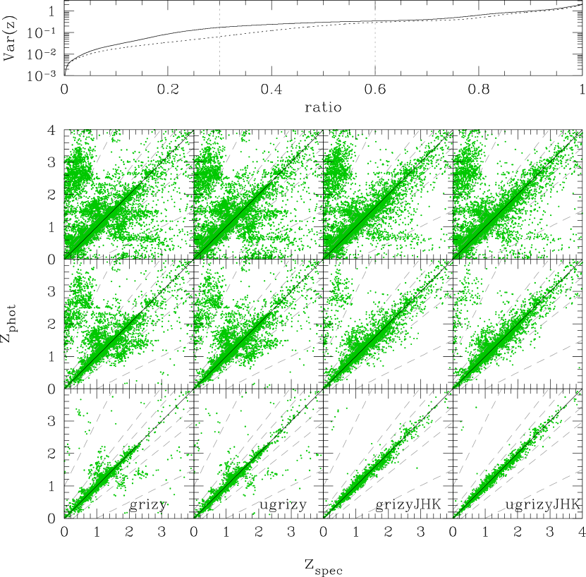
Figure 6.— Lower plot: The scatter plots between photometric and true redshifts for our simulated galaxies. The different columns correspond to the results for different sets of filters as indicated in the bottom panels, while the different rows correspond to different object selections (see § 4.3 for the details). The upper-row panels show the results of samples containing all the galaxies with $i<25.8$ that have their photo-$z$ fits quantified as $\chi^{2}_{\nu}\leq 2$ (see Eq. [10]). The middle- and bottom-row panels show the results of subsamples obtained by discarding 40% and 70% galaxies with ill-defined photo-$z$ estimates, respectively. This is done by choosing the threshold value ${\rm Var}(z)$ (see Eq. [11]) for each galaxy such that the desired fractions of galaxies are remained in the resulting subsamples. Note that, for illustrative purpose, only 5% representative galaxies in each subsample are shown in each plot. Upper panel: The ratio of remaining galaxies that have ${\rm Var}(z)$ values greater than a given threshold denoted on the vertical axis. The solid curve shows the result for the set of filters, $grizy$, while the dotted curve shows the result when the NIR data $JHK$ are added (see Table 1 for the details). Note that the results are almost unchanged by further adding the $u$-band data. The vertical thin dashed lines denote the selections used in the lower plot, the criteria discarding 40% and 70% galaxies with poor photo-$z$’s.

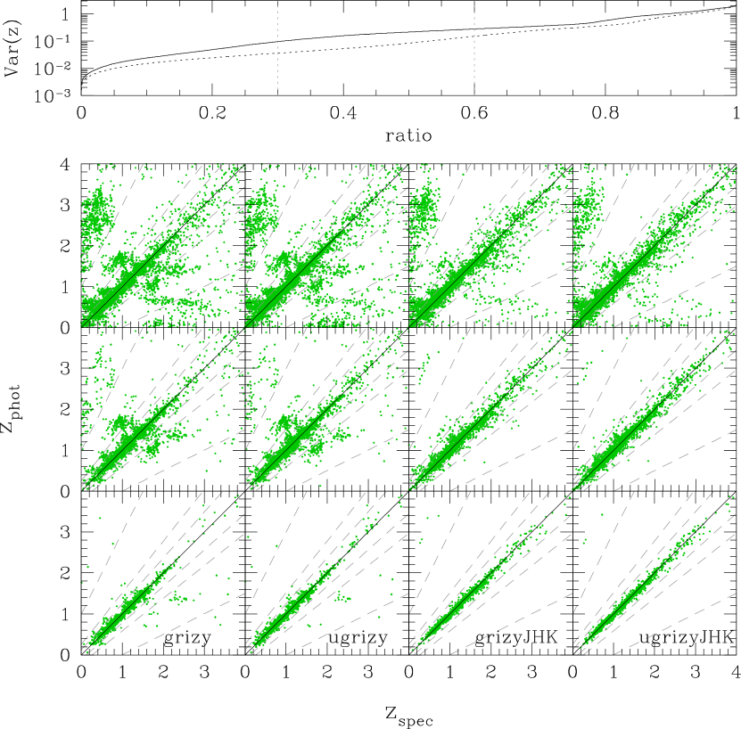
Figure 7.— Similar to Figure 6, but for the different range of $i$-band magnitudes for object selection, $22.5<i<25$.

Figure 7 shows the similar result to the previous figure, but for brighter samples of galaxies, selected with $i<25$ or equivalently with $S/N$ values greater than $10\sigma$ in $i$-band. These brighter galaxies are more suitable for the accurate shape measurement as discussed in § 4.3. One can find that the photo-$z$ accuracy is improved compared to Figure 6.

5.2. Simulating Lensing Tomography: The Impact of Photo-$z$ Errors

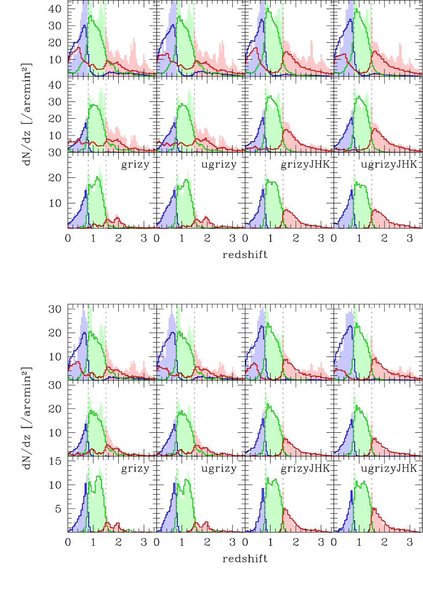
Figure 8.— The shaded histograms are the redshift distributions of galaxies based on their photo-$z$ information, i.e. the sharp cuts imposed on the photo-$z$’s: $0<z_{p}<0.8$, $0.8<z_{p}<1.5$ and $z_{p}>1.5$, indicated on the vertical dashed lines. In this case the horizontal axis denotes photo-$z$ values. The solid-line histograms are the underlying true distributions, therefore the horizontal axis denotes true redshifts in this case. The upper and lower panels are the results using the galaxy catalogs in Figures 6 and 7, respectively. The different panels are for different galaxy selections as in Figures 6 and 7.

We are now in a position to use the photo-$z$ galaxy catalogs, constructed up to the preceding section, to make the trade-off analysis on the number of galaxies within a sample versus how “clean” the tomographic redshift intervals are. Then we study the impact of photo-$z$ errors on parameter estimation assuming the hypothetical lensing tomography experiment.

Figure 8 shows the redshift distributions of each tomographic bin made by subdividing the photo-$z$ galaxies into 3 intervals of photometric redshifts, $z_{p}<0.8$, and $0.8<z_{p}<1.5$ and $z_{p}>1.5$. The redshift intervals are chosen such that each redshift intervals contain similar number densities for the original mock catalog of galaxies. Note that the redshift binning is fixed in the following analysis for simplicity, which helps to compare the results of different galaxy catalogs. Also note that three redshift bins are a minimal choice of lensing tomography for constraining the dark energy equation of state parameter “$w$” to a reasonable accuracy by efficiently breaking parameter degeneracies in the lensing power spectrum (e.g. Takada & Jain, 2004).

The upper plot in Figure 8 shows the tomographic redshift distributions constructed from different photo-$z$ catalogs in Figure 6, where different panels correspond to the different sets of filters and the different clipping thresholds. The shaded regions in each panel show the photometric redshift distributions of galaxies, which have sharp cutoffs in the distributions due to the sharp redshift binning, while the solid line histograms show the underlying true redshift distributions. As can be found from the top-row panels, if all the galaxies are used, the resulting redshift distributions have significant overlaps between different redshift bins due to a significant contamination of photo-$z$ outliers for any combinations of filters. On the other hand, the middle- and bottom-row panels show that, when 40% or 70% of photo-$z$ outliers are discarded by imposing the corresponding thresholds on ${\rm Var}(z)$, respectively, the overlaps can be increasingly reduced. In particular, when the optical data is combined with the NIR data such that those expected from the VIKING survey, the resulting subsamples have almost no overlap, if about $70\%$ of galaxies are discarded. We should note that such a clean redshift binning can greatly reduce a possible contamination of the intrinsic ellipticity alignments arising from the physically close pairs of galaxies in the similar redshifts (Takada & White, 2004).

The lower plot shows the similar results for higher $S/N$ samples with $22.5<i<25$ whose scatter plots are seen in Figure 7. Again, if using the clipping method and having a wider coverage of wavelengths, a clean subsample with almost no overlap between redshift bins can be obtained.

As have been stressed several times, the weak lensing power spectra are, to the zero-th order approximation, sensitive to the mean redshifts of each redshift bins, and less to the statistical errors of photo-$z$’s or the detailed shape of redshift distribution. The level of systematic photo-$z$ errors in each tomographic bins is quantified in Figure 9. The central values and error bars in this plot show the bias in mean redshift and the statistical error of the mean redshift, $\sigma(\langle\Delta z\rangle)$, where $\Delta z$ is defined before (see around Fig. 5) and the average $\langle\cdots\rangle$ denotes the average over all the galaxies in the tomographic redshift bin. Note that, for illustrative purpose, the error bars are scaled for a survey area of $1$ arcmin², and therefore the corresponding errors for our fiducial survey area of 2000 sq. degrees are much smaller than plotted, by a factor of $\sqrt{2000\times 60^{2}}\simeq 2700$.

The middle- and bottom-row panels are the results of subsamples obtained by further imposing the condition $0.2\leq z_{p}\leq 1.5$ or $22.5\leq i\leq 25$, respectively. It is clear that, without clipping ill-defined photo-$z$ galaxies, the bias and errors are significant. Note that the redshift bias for no tomography case sometimes becomes smaller than in some tomographic bins (especially highest redshift bins), because photo-$z$ outliers at low- and high-redshifts cancel out to some extent in no tomography case. As can be seen from the middle-row panels, when the restricted redshift range of $0.2<z<1.5$ is considered, a subsample with most accurate photo-$z$’s is obtained, because spectral features of galaxies, especially the Lyman and 4000 Å  breaks, are well captured by the sets of filters in this redshift range.

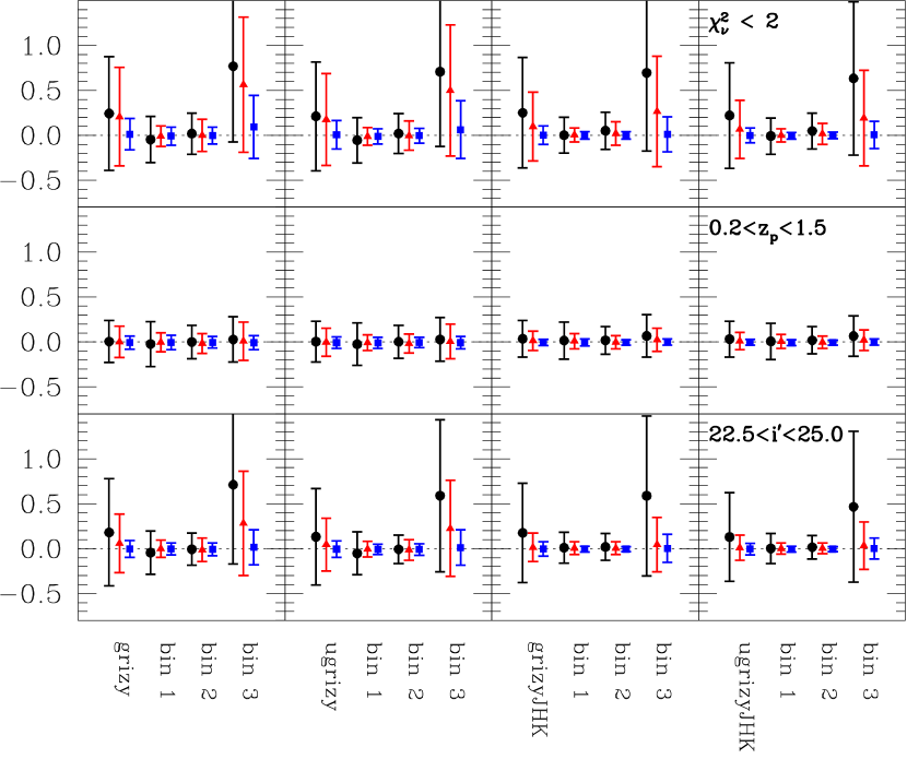
Figure 9.— The bias between photometric and true redshifts, $\langle\Delta z\rangle$, in each tomographic redshift interval. The error around each point is the statistical error of the mean redshift, $\sigma(\langle\Delta z\rangle)$, in each redshift bin. For illustrative purpose, the errors are for a survey area of 1 sq. arcminutes, and the errors are smaller by a factor $\sqrt{2000\times 60^{2}}\simeq 2700$ for our fiducial survey area of 2000 sq. degrees. The panels in different columns show the results for different sets of filters as indicated on the horizontal axis. The upper-row panels are for the subsamples where galaxies with $i<25.8$ are selected only with the condition $\chi^{2}_{\nu}<2$. The middle- and bottom-row panels are for the subsamples where the condition $0.2<z_{p}<1.5$ or $22.5<i<25$ is further imposed for the selection, respectively. The round symbols in each panel show the results for the whole galaxy sample, while the triangle and square symbols are the results for the subsamples discarding 40% and 70% of galaxies with ill-defined photo-$z$’s, respectively, based on our clipping method. In each panel the four symbols are for different redshift intervals: “bin1”, “bin2”, and “bin3” correspond to the lowest, medium and highest redshift bins in Figure 8, and the leftmost symbols are for the case of no tomography, i.e. a single redshift interval.

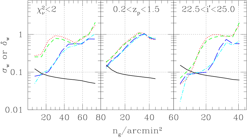
Figure 10.— The forecasted constraints on the dark energy equation of state parameter $w$ as a function of number densities of galaxies included in the corresponding galaxy catalogs, expected for the lensing tomography experiment with survey area of $2000$ deg² in combination with the Planck CMB information. The three redshift bins are considered for each galaxy subsamples as in Figure 8. The solid curve in each panel shows the marginalized error $\sigma(w)$ assuming no photo-$z$ errors. The other curves show the offset bias of the best-fit $w$ from the true value ($w=-1$), computed by using the Fisher matrix formalism (see around Eq. [LABEL:eq:bias_theta_red]): the dotted, dashed, long-dashed and dot-dashed curves are for combinations of filters, $grizy$, $ugrizy$, $grizyJHK$ and $ugrizyJHK$, respectively. The left, middle and right panels are the results for different object selections as in Figure 8.

Figure 11.— As in the previous figure, but the results obtained by artificially discarding photo-$z$ outliers given as $\log(1+z_{p})/(1+z_{s})\geq\pm 0.1$, $0.3$ and $0.5$ (the three dotted curves from top to bottom, respectively). The filter combination $grizy$ is considered in this plot. For comparison the top dashed curve in each panel is the same as the dotted curve in Figure 10.

We next propagate the errors of tomographic redshifts into the dark energy parameter $w$, expected from the lensing power spectrum measurements, based on the Fisher matrix formalism described in § 4.2. To do this we address the following questions:

• The trade-off of dark energy constraint: the statistical accuracy of $w$, $\sigma(w)$, versus the offset of the best-fit value from the true value, $\delta w$.

• Study the dark energy trade-off against different subsamples of galaxies.

These can be studied by using the simulated galaxy catalogs. The statistical error of $w$ can be reduced by including more number of galaxies in the sample for a fixed range of working multipoles ($5\leq\ell\leq 3000$), because the shot noise is more suppressed. On the other hand, a bias in the best-fit $w$ due to the photo-$z$ errors can be reduced by discarding photo-$z$ outliers, leaving a fewer number of galaxies in the subsample. Hence a trad-off point in $\sigma(w)$ versus $\delta w$ may be found by compromising these competing effects.

Figure 10 shows the marginalized error $\sigma(w)$ and the amount of bias $|\delta w|$ as a function of number densities of galaxies included in the corresponding galaxy subsamples. Again note that we considered the lensing tomography with three tomographic bins for a sky coverage of 2000 square degrees. The smaller number densities in the horizontal axis correspond to subsamples of galaxies where more galaxies with ill-defined photo-$z$’s are discarded by imposing more stringent thresholds on ${\rm Var}(z)$, i.e. smaller threshold values of ${\rm Var}(z)$, in the clipping method. The different curves are for different combinations of filters. The error $\sigma(w)$ is computed from the underlying true redshift distribution, i.e. for the case with perfect photo-$z$’s, therefore specified by the number density in the horizontal axis. When $\delta w\geq\sigma(w)$, the best-fit value of $w$ can be away from the true one by more than the $1\sigma$ error; even if the true model has the cosmological constant ($w=-1$), the result of $w\neq-1$ may be falsely inferred. Hence a minimal requirement on photo-$z$ accuracies can be assessed from the condition $\delta w\leq\sigma(w)$.

First, the plot shows that, as the subsample is restricted to galaxies with more accurate photo-$z$’s, i.e. the smaller number densities, the bias in $w$ is reduced to some extent. On the other hand, the error $\sigma(w)$ is only slightly degraded because the constraint comes mainly from the sample variance limited regime for a given range of working multipoles ($5\leq l\leq 3000$).

It is also shown that the bias can be reduced by adding the NIR- and/or u-band data. However, the broadband data alone may not be sufficient to reduce the bias. The optimal range of redshifts needs to be considered, and a brighter subsample whose galaxies have higher $S/N$ values in each filter is preferred to sufficiently reduce the bias, as implied from the middle and right panels. Depending on the available set of filters, the compromising point can be obtained around the number densities $\bar{n}_{g}=[10,30]$ arcmin^-2, i.e. more than 60% of ill-defined photo-$z$ galaxies need to be discarded. It would also be worth noting that combining the lensing constraints with other dark energy probes such as the baryon acoustic oscillation experiment may allow to further calibrate photo-$z$ errors by breaking parameter degeneracies.

We have so far paid special attention to how to eliminate photo-$z$ outliers in order to obtain a subsample of galaxies suitable for tomographic lensing measurements. However, due to the limitation of photo-$z$ accuracies, there may remain a residual bias in the tomographic redshift bins, even if photo-$z$ outliers are completely removed. To study this, Figure 11 shows the results obtained by artificially discarding photo-$z$ outliers according to the clipping criteria

$$\log\frac{1+z_{p}}{1+z_{s}}>\pm t,$$ (14)

with $t=0.1,0.3$ and $0.5$, respectively. The figure shows that a bias in $w$ cannot be fully eliminated even if the outliers are completely discarded. This implies that there remains a residual bias in the mean redshift for each tomographic bins due to asymmetric photo-$z$ errors around $z_{p}=z_{s}$, therefore the residual biases would need to be calibrated, e.g. by using a spectroscopic training subsample (e.g. Ma & Bernstein, 2008).

5.3. Angular cross-correlations of galaxies between different photo-$z$ bins

An alternative way to identify photo-$z$ outliers is using angular cross-correlations of galaxies between different photo-$z$ bins (Newman, 2008; Erben et al., 2009; Zhang et al., 2009; Schulz, 2009). As implied in Fig. 8, photo-$z$ errors cause overlaps of galaxies between different redshift bins. Therefore photo-$z$ errors may cause non-vanishing cross-correlations of galaxies between different photo-$z$ bins, if the galaxies indeed have similar true redshifts, therefore are physically correlated with each other. In other words the cross-correlations can, albeit statistical, be used to monitor a contamination of photo-$z$ outliers. In this subsection we use our simulated photo-$z$ catalogs to estimate the expected signal-to-noise ratios for measuring the cross-correlations assuming the same survey parameters we have considered.

Assuming the Limber approximation, the angular power spectra of galaxies in the $i$- and $j$-th photo-$z$ bins are given as

$$C^{gg}_{ij}(\ell)=\int_{0}^{\infty}\!\!dz\frac{dz}{d\chi}\frac{b_{i}b_{j}}{\chi^{2}}\frac{n_{i}(z)n_{j}(z)}{\bar{n}_{i}\bar{n}_{j}}P_{\delta}\!\!\left(\frac{\ell}{\chi},z\right)+\frac{\delta_{ij}^{K}}{\bar{n}_{i}},$$ (15)

where $n_{i}(z)$ is the underlying true redshift distribution for the $i$-th photo-$z$ bin and $\bar{n}_{i}$ is its mean number density. In the following we consider a sharp redshift binning in photo-$z$ space, however, the underlying true distributions generally have overlaps due to photo-$z$ errors. We here simply assume that the galaxy distribution in the $i$-th bin is related to the matter distribution via constant bias parameter $b_{i}$, which is taken to $b_{i}=1$ for all the photo-$z$ bins for simplicity. To make this assumption reasonable, we restrict the following analysis to a range of low multipoles $l<500$. Notice that the cross power spectra are not affected by shot noise.

The strength of cross-correlations or redshift leakages can be quantified by the cross-correlation coefficients at each multipole:

$$\mu_{ij}(\ell)=\frac{C_{ij}^{gg}(\ell)}{\sqrt{C_{ii}^{gg}(\ell)C_{jj}^{gg}(\ell)}}.$$ (16)

The coefficient $\mu_{ij}\simeq 1$ implies significant cross-correlations between the $i$- and $j$-th bins compared to their auto-spectra, while $\mu_{ij}=0$ means no cross-correlation or no leakage of photo-$z$ outliers into different bins. The total signal-to-noise ratios expected for measuring the cross-correlations can be estimated as

$$\left(\frac{S}{N}\right)^{2}_{ij}\equiv\sum_{\ell=\ell_{\rm min}}^{\ell_{\rm max}}f_{\rm sky}(2\ell+1)\frac{C_{ij}^{2}}{C_{ij}^{2}+C_{ii}C_{jj}}.$$ (17)

Here we simply assume the Gaussian covariances to model the statistical errors in measuring cross power spectra from a survey. Note that the error covariance includes the shot noise contamination via the auto spectra $C_{ii}$ and $C_{jj}$. As for the minimum and maximum multipoles used in the summation, we adopt $\ell_{\rm min}=5$ and $\ell_{\rm max}=500$, respectively.

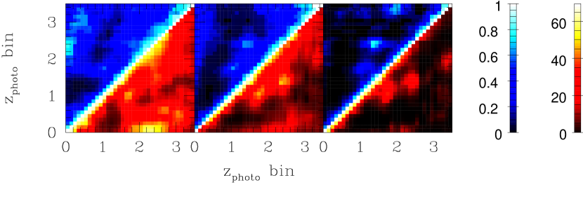
Figure 12.— Angular cross-correlations between galaxies in two photo-$z$ bins, denoted on the horizontal and vertical axes, for our fiducial survey with 2000 square degrees, adopting 35 redshift bins over $0<z_{p}<3.5$ with the bin width $dz=0.1$. As in Fig. 6, the left panel shows the result for galaxy catalog selected with $ugrizy$ and $\chi^{2}_{\nu}<2$, while the middle- and right-panels show the results for the catalogs where 40% and 70% of galaxies with ill-defined photo-$z$’s are discarded. The upper-left off-diagonal components in each panel show the correlation coefficients $\mu_{ij}$ (see Eq. [16]) at multipole $\ell=100$. Compared with Fig. 6, one can find photo-$z$ outliers cause “island” regions with high coefficients $\mu_{ij}\simeq 1$. The lower-right components show the cumulative signal-to-noise ratios $(S/N)$ expected in measuring the cross-power spectrum over a range of multipoles $5\leq\ell\leq 500$. Again the cross-correlations between different bins, caused by photo-$z$ outliers, show high $S/N$ values greater than 10.

Figure 12 studies the angular cross-correlations for our fiducial survey parameters with 2000 square degree coverage. Here we consider the photo-$z$ galaxy catalog selected with $ugrizy$ and $\chi^{2}_{\nu}<2$, and adopt 35 redshift bins over $0<z_{p}<3.5$ with the bin width $dz=0.1$ corresponding to a typical photo-$z$ error on individual galaxy basis. The upper-left triangle in each panel shows the correlation coefficients of cross-power spectra between the two different photo-$z$ bins, $\mu_{ij}$. The coefficients have large values around the diagonal terms, i.e. $z_{pi}\simeq z_{pj}$, because the photo-$z$ errors cause significant overlaps between neighboring redshift bins. Compared with the results in Fig. 6, one can find that photo-$z$ outliers cause some isolated regions with significant correlation coefficients.

The lower-right triangle shows the expected signal-to-noise ratios, $S/N$, for measuring cross-correlations. The sufficiently high $S/N$ values, say greater than 10, can be expected for redshift bins that have high correlation coefficients. Thus monitoring the cross-correlations between different photo-$z$ bins may allow to further identify photo-$z$ outliers, in a statistical sense. However, the genuine power of cross-correlation method for eliminating the outliers or calibrating the photo-$z$ errors needs to be more carefully studied.

Finally we remark on a more quantitative work done in Schulz (2009), which studied, based on mock simulations, the use of cross-correlations of photometric galaxies with an overlapping spectroscopic sample to calibrate the redshift distribution of the photometric galaxies without using the photo-$z$ information. While the main purpose of this paper is not using the cross-correlations to identify photo-$z$ outliers, the promising result shown is that the redshift distribution can be well reconstructed by using a sufficiently large spectroscopic sample. However, one of the limiting factors realized is the reconstruction requires a sufficiently fine binning of spectroscopic redshifts, which tends to make the cross-correlation measurements noisy. Therefore it would be interesting to study how the method can be further refined by combining the cross-correlation method and the photo-$z$ information, and the combined method may relax a requirement on the size of spectroscopic calibration sample. We also note that, as pointed out in Bernstein & Huterer (2009), the cross-correlation method is affected by the lensing magnification bias, which may cause an apparent correlations between foreground and background galaxies even if there is no photo-$z$ errors to cause redshift overlaps. This effect also needs to be included, and mock simulations would be useful for such a study on the cross-correlation method.

6. Summary and Discussion

In this paper we have studied how photo-$z$ errors available from broadband multi-color data affect cosmological parameter estimation obtained from tomographic lensing experiment. To do this, we made the simulated mock galaxy catalog with photo-$z$ information constructed from the COSMOS catalog. Since the photo-$z$ errors are sensitive to survey parameters such as available filters, the depths, and so on, we considered in this paper the survey parameters to resemble the planned Subaru Hyper Suprime-Cam survey, which is characterized by the optical multi-passband data ($grizy$) and the depth $i\lower 2.15277pt\hbox{$\;\buildrel<\over{\sim}\;$}26$. We also studied how the photo-$z$ accuracy can be improved if combining the optical data with the $u$-band data expected from a CFHT-type telescope and the NIR ($JHK$) data from the VIKING-type survey. However, the method developed in this paper can be readily extended to other weak lensing surveys.

We particularly paid our attention to how to construct a galaxy subsample suitable for weak lensing tomography. We showed that photo-$z$ outliers can be efficiently identified by monitoring the posterior likelihood of redshift estimation for each galaxy: more exactly, the width of likelihood function defined by the second moment around the best-fit redshift parameter (see Eq. [11]) was used as an indicator of the photo-$z$ accuracy on individual galaxy basis. It was also shown that the photo-$z$ outliers can be more efficiently removed by restricting the ranges of working magnitudes and/or redshifts, and adding the $u$- and $NIR$ bands (see Figs. 6–9).

Using the Fisher matrix formalism, we estimated how the photo-$z$ errors in a defined galaxy catalog cause biases in cosmological parameters, especially the dark energy equation of state parameter $w$. It was shown how the parameter biases can be reduced with discarding galaxies with ill-defined photo-$z$ estimates. However, with discarding more galaxies, the statistical accuracies of parameters are degraded due to the increased shot noise contamination. We found that the trade-off point, where the parameter bias becomes similar or smaller than the marginalized statistical error, can be achieved if a large fraction of ill-defined photo-$z$ galaxies ($\sim 70\%$) are discarded and if combined with the $u$- and NIR-band data sets (Fig. 10).

However, as demonstrated in Fig. 11, even if photo-$z$ outliers are completely eliminated, there may remain a non-negligible, residual bias in the mean redshift of each tomographic bin because the scatters around the relation between photometric and true redshifts, $z_{p}=z_{s}$, are not necessarily symmetric and therefore not perfectly canceled even after the average of galaxies in each redshift bin. Therefore a careful calibration of the residual photo-$z$ errors will be inevitably needed for any future surveys (Hearin et al., 2010).

A powerful method for the photo-$z$ calibration is using a training spectroscopic subsample. Naively, if a fair, representative spectroscopic subsample of imaging galaxies used in the lensing analysis is available, it allows a calibration of photo-$z$ errors. However, the size of such a spectroscopic sample required for achieving the meaningful dark energy constraint becomes very large; for a lensing survey with sky coverage of more than 1000 sq. degrees, containing more than $10^{8}$ imaging galaxies, a subsample with more than $10^{6}$ spectroscopic redshifts is required (Huterer et al., 2006; Ma et al., 2006). Note that the currently largest redshift sample is given by the COSMOS project containing $10^{4}$ redshifts. Thus a survey collecting $10^{6}$ spectra, which is required for our sample fully calibrated, is observationally very expensive and almost infeasible, especially if redshifts of faint galaxies are needed (but see Bernstein & Huterer, 2009, for relaxing the requirement).

On the other hand, there is a new method recently proposed (Mandelbaum et al., 2008; Lima et al., 2008; Cunha et al., 2009), using a spectroscopic subsample of smaller size, which is not necessarily a fair, representative subsample of imaging galaxies. First spectroscopic galaxies are compared to imaging galaxies in multi-dimensional color space, rather than the photo-$z$ space. Secondly the ratio between number densities of spectroscopic and imaging galaxies is computed at each point in multi-color space. Then the ratio is multiplied to the redshift distribution of spectroscopic subsample to infer the underlying redshift distribution of imaging galaxies. Thus this weighting method may allow the photo-$z$ calibration using a spectroscopic subsample of smaller size. However, there is still an open issue to be carefully investigated in this method. For example, it is unclear how the calibration degrades if the spectroscopic subsample has significant sample variance fluctuations in the redshift distribution, e.g. due to clustering contamination at particular redshifts due to a finite area coverage.

Another calibration method is using cross-correlations of galaxies in photo-$z$ bins, as partly studied in Fig. 12. Again the non-vanishing cross-correlations only arise when the photo-$z$ errors cause leakages into different bins of true redshifts. Or spectroscopic galaxies in the same survey region, if available, can also be used to cross-correlate with imaging galaxies in order to calibrate the photo-$z$ errors over a range of redshifts covered by the spectroscopic sample (Newman, 2008; Schulz, 2009). However spectroscopic galaxies may be correlated with only particular types of galaxies, therefore, this method may have a limitation. Hence it would be interesting to explore how to calibrate the redshift distribution of imaging galaxies down to the required accuracy level by combining various methods, the method developed in this paper and the methods based on spectroscopic subsample or/and cross-correlation measurements.

Finally we comment on another important contaminating effect, the intrinsic alignment in galaxy shapes (e.g. Hirata & Seljak, 2004; Mandelbaum et al., 2006, 2009). As studied in detail in King & Schneider (2003) (also see Heymans & Heavens, 2003; Takada & White, 2004; Bridle & King, 2007), accurate photo-$z$ information is needed to calibrate and/or correct for the intrinsic alignment contamination in weak lensing tomography. A subsample with reliable photo-$z$’s, constructed based on the method in this paper, may be also useful for this purpose.

References

- Abdalla et al. (2008) Abdalla, F. B., Amara, A., Capak, P., Cypriano, E. S., Lahav, O., & Rhodes, J. 2008, MNRAS, 387, 969
- Bartelmann & Schneider (2001) Bartelmann, M., & Schneider, P. 2001, Phys. Rep., 340, 291
- Benítez (2000) Benítez, N. 2000, ApJ, 536, 571
- Bernstein & Huterer (2009) Bernstein, G., & Huterer, D. 2009, MNRAS, 1648
- Bolzonella et al. (2000) Bolzonella, M., Miralles, J.-M., & Pelló, R. 2000, A&A, 363, 476
- Bordoloi et al. (2009) Bordoloi, R., Lilly, S. J., & Amara, A. 2009, ArXiv e-prints
- Bridle & King (2007) Bridle, S., & King, L. 2007, New Journal of Physics, 9, 444
- Bruzual & Charlot (2003) Bruzual, G., & Charlot, S. 2003, MNRAS, 344, 1000
- Bruzual & Charlot (1993) Bruzual, G., A., & Charlot, S. 1993, ApJ, 405, 538
- Calzetti et al. (2000) Calzetti, D., Armus, L., Bohlin, R. C., Kinney, A. L., Koornneef, J., & Storchi-Bergmann, T. 2000, ApJ, 533, 682
- Collister & Lahav (2004) Collister, A. A., & Lahav, O. 2004, PASP, 116, 345
- Cunha et al. (2009) Cunha, C. E., Lima, M., Oyaizu, H., Frieman, J., & Lin, H. 2009, MNRAS, 396, 2379
- Erben et al. (2009) Erben, T., et al. 2009, A&A, 493, 1197
- Fu et al. (2008) Fu, L., et al. 2008, A&A, 479, 9
- Hearin et al. (2010) Hearin, A. P., Zentner, A. R., Ma, Z., & Huterer, D. 2010, ArXiv e-prints
- Heymans & Heavens (2003) Heymans, C., & Heavens, A. 2003, MNRAS, 339, 711
- Hirata & Seljak (2004) Hirata, C. M., & Seljak, U. 2004, Phys. Rev. D, 70, 063526
- Hoekstra & Jain (2008) Hoekstra, H., & Jain, B. 2008, Annual Review of Nuclear and Particle Science, 58, 99
- Hu (1999) Hu, W. 1999, ApJ, 522, L21
- Huterer (2002) Huterer, D. 2002, Phys. Rev. D, 65, 063001
- Huterer (2010) Huterer, D. 2010, ArXiv e-prints
- Huterer & Takada (2005) Huterer, D., & Takada, M. 2005, Astroparticle Physics, 23, 369
- Huterer et al. (2006) Huterer, D., Takada, M., Bernstein, G., & Jain, B. 2006, MNRAS, 366, 101
- Ilbert et al. (2009) Ilbert, O., et al. 2009, ApJ, 690, 1236
- Jain et al. (2007) Jain, B., Connolly, A., & Takada, M. 2007, Journal of Cosmology and Astro-Particle Physics, 3, 13
- Joachimi & Schneider (2009) Joachimi, B., & Schneider, P. 2009, ArXiv e-prints
- Jouvel et al. (2010) Jouvel, S., et al. 2010, ArXiv e-prints
- King & Schneider (2003) King, L. J., & Schneider, P. 2003, A&A, 398, 23
- Komatsu et al. (2009) Komatsu, E., et al. 2009, ApJS, 180, 330
- Lewis & Challinor (2006) Lewis, A., & Challinor, A. 2006, Phys. Rep., 429, 1
- Lima et al. (2008) Lima, M., Cunha, C. E., Oyaizu, H., Frieman, J., Lin, H., & Sheldon, E. S. 2008, MNRAS, 390, 118
- Ma & Bernstein (2008) Ma, Z., & Bernstein, G. 2008, ApJ, 682, 39
- Ma et al. (2006) Ma, Z., Hu, W., & Huterer, D. 2006, ApJ, 636, 21
- Mandelbaum et al. (2009) Mandelbaum, R., et al. 2009, ArXiv e-prints
- Mandelbaum et al. (2006) Mandelbaum, R., Hirata, C. M., Ishak, M., Seljak, U., & Brinkmann, J. 2006, MNRAS, 367, 611
- Mandelbaum et al. (2008) Mandelbaum, R., et al. 2008, MNRAS, 386, 781
- Massey et al. (2010) Massey, R., Kitching, T., & Richard, J. 2010, ArXiv e-prints
- Miller & Scalo (1979) Miller, G. E., & Scalo, J. M. 1979, ApJS, 41, 513
- Miyazaki et al. (2006) Miyazaki, S., et al. 2006, in Presented at the Society of Photo-Optical Instrumentation Engineers (SPIE) Conference, Vol. 6269, Society of Photo-Optical Instrumentation Engineers (SPIE) Conference Series
- Miyazaki et al. (2002) Miyazaki, S., et al. 2002, PASJ, 54, 833
- Mobasher et al. (2004) Mobasher, B., et al. 2004, ApJ, 600, L167
- Newman (2008) Newman, J. A. 2008, ApJ, 684, 88
- Okabe et al. (2009) Okabe, N., Takada, M., Umetsu, K., Futamase, T., & Smith, G. P. 2009, ArXiv e-prints
- Rudd et al. (2008) Rudd, D. H., Zentner, A. R., & Kravtsov, A. V. 2008, ApJ, 672, 19
- Sawicki et al. (1997) Sawicki, M. J., Lin, H., & Yee, H. K. C. 1997, AJ, 113, 1
- Schulz (2009) Schulz, A. E. 2009, ArXiv e-prints
- Seljak & Zaldarriaga (1996) Seljak, U., & Zaldarriaga, M. 1996, ApJ, 469, 437
- Smith et al. (2003) Smith, R. E., et al. 2003, MNRAS, 341, 1311
- Takada & Bridle (2007) Takada, M., & Bridle, S. 2007, New Journal of Physics, 9, 446
- Takada & Jain (2004) Takada, M., & Jain, B. 2004, MNRAS, 348, 897
- Takada & Jain (2009) Takada, M., & Jain, B. 2009, MNRAS, 395, 2065
- Takada & White (2004) Takada, M., & White, M. 2004, ApJ, 601, L1
- Wittman (2009) Wittman, D. 2009, ApJ, 700, L174
- Wolf (2009) Wolf, C. 2009, MNRAS, 397, 520
- Zentner et al. (2008) Zentner, A. R., Rudd, D. H., & Hu, W. 2008, Phys. Rev. D, 77, 043507
- Zhang et al. (2009) Zhang, P., Pen, U., & Bernstein, G. 2009, ArXiv e-prints