Telling time with an intrinsically noisy clock

Abstract

Intracellular transmission of information via chemical and transcriptional networks is thwarted by a physical limitation: the finite copy number of the constituent chemical species introduces unavoidable intrinsic noise. Here we provide a method for solving for the complete probabilistic description of intrinsically noisy oscillatory driving. We derive and numerically verify a number of simple scaling laws. Unlike in the case of measuring a static quantity, response to an oscillatory driving can exhibit a resonant frequency which maximizes information transmission. Further, we show that the optimal regulatory design is dependent on the biophysical constraints (i.e., the allowed copy number and response time). The resulting phase diagram illustrates under what conditions threshold regulation outperforms linear regulation.

It has long been recognized Berg and Purcell (1977) that the ability to measure biochemical quantities, e.g., concentrations, is intrinsically thwarted by the small copy numbers present at the scale of the cell. This observation has launched considerable experimental investigations as to how high-fidelity signal transmission can occur within single cells Mettetal et al. (2008); Elowitz and Leibler (2000), along with an associated literature in mathematical and computational techniques for modeling such noisy information transmission Tostevin and ten Wolde (2009); Tănase-Nicola et al. (2006); Tkacik et al. (2008). From the perspective of biological design – either to understand the mechanisms which lead to observed biology or to create synthetic systems with desirable properties – these works investigate how regulatory elements which comprise biological systems function in the presence of intrinsic noise Bialek and Setayeshgar (2005).

In earlier work we showed how the ‘spectral method’ leads to an efficient and accurate numerical technique, which permits optimization to reveal the information-optimal design of a transcriptional cascade in the presence of intrinsic noise in the statistical steady-state Walczak et al. (2009); Mugler et al. (2009). We here turn our attention to the simplest model of the dynamic case, illustrated in Fig. 1(a), in which a single transcription factor (the ‘parent’) with copy number $n$ is driven by an oscillatory creation rate $f(t)=g+\alpha\cos\omega t$ and regulates the expression of a second species (the ‘child’) with copy number $m$; the regulation is modeled via the child’s creation rate $q_{n}$. This model captures the noisy downstream response to oscillation, e.g., the cell cycle, without limiting the results to a particular mechanism for generating oscillations (e.g., via cell division Csikász-Nagy et al. (2006), repressive cycles Elowitz and Leibler (2000), or activation-repression circuits Cookson et al. (2009)). We show how the optimal design – i.e., the choice of linear-vs.-cooperative and up-vs.-down regulation – is determined by the physical demands in terms of allowed copy number and response time. Further, while our intuition from understanding how best to measure static signals suggests that slower response time is always more accurate Berg and Purcell (1977), we illustrate how oscillatory driving leads to an information-optimal driving frequency, and compute how this frequency depends on copy number.

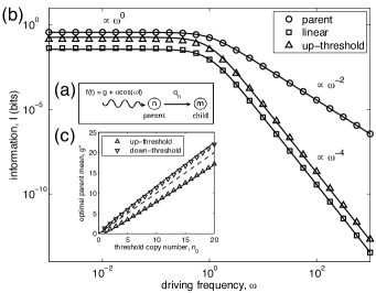
Figure 1: (a) A transcription factor (the ‘parent’) with copy number $n$ is driven by an oscillatory creation rate $f(t)=g+\alpha\cos\omega t$ and regulates via $q_{n}$ the expression of a second species (the ‘child’) with copy number $m$. (b, c) Numerical confirmations (data points) of analytic expressions (lines) derived in the small-information limit: Eqns.  9 (circles) and 13 top line (squares) and bottom line (triangles) in (b), and Eqn. 14 for both up- (up-triangles) and down-regulation (down-triangles) in (c). Parameters are $g=n_{0}=1$ and $c=0.1$ for (b), $\omega=1$ for (c), and $\alpha=\rho=\Delta=1$ and $q_{0}=0$ for both, yielding small parameters $|\nu_{1}|\leq 0.5$ (Eqn. 5), $|\mu_{1}|\leq 0.05$ (linear;  Eqn. 12) and $|\mu_{1}|\leq 0.184$ (threshold;  Eqn. 12).

In the spectral method Walczak et al. (2009) we exploit the linearity of the master equation ${\dot{p}}_{nm}=-\left({\cal L}_{n}[f(t)]+\rho{\cal L}_{m}[q_{n}]\right)p_{nm}$, the equation of motion for the joint probability of observing $n$ and $m$ copies of the parent and child, respectively, and expand its solution in terms of the natural eigenfunctions of the birth-death process with constant creation and decay. For a birth-death process expressed in terms of an arbitrary creation rate $h$ on species $s$ the positive semidefinite operator ${\cal L}_{s}$ acts as ${\cal L}_{s}[h]p_{s}=sp_{s}-(s+1)p_{s+1}+hp_{s}-hp_{s-1}$; time is normalized via the parent decay rate (in these units $\rho$ is the child decay rate). To study dynamics we also Fourier transform in harmonics of the driving frequency $\omega$,

$${p}_{nm}(t)=\sum_{j=0}^{\infty}\sum_{k=0}^{\infty}\sum_{z=-\infty}^{\infty}p_{jk}^{z}\langle n|j\rangle\langle m|k\rangle{\rm e}^{-iz\omega t},$$ (1)

where the parent and child eigenfunctions (or ‘spectral modes’) enjoy ${\cal L}_{n}[g]\langle n|j\rangle=j\langle n|j\rangle$ and ${\cal L}_{m}[{\bar{q}}]\langle m|k\rangle=k\langle m|k\rangle$, respectively. Just as in Mugler et al. (2009); Walczak et al. (2009), we introduce a gauge ${\bar{q}}$ to define the basis; the analytic results below are independent of this choice.

The master equation then becomes an algebraic relation among the expansion coefficients $p_{jk}^{z}$:

$$-i\omega zp_{jk}^{z}=-(j+\rho k)p_{jk}^{z}+\frac{\alpha}{2}\sum_{\pm}p_{j-1,k}^{z\pm 1}-\rho\sum_{j^{\prime}}\Delta_{jj^{\prime}}p_{j^{\prime},k-1}^{z},$$ (2)

where $\Delta_{jj^{\prime}}=\sum_{n}\langle j|n\rangle(\bar{q}-q_{n})\langle n|j^{\prime}\rangle$. Algorithmically we (i) initialize with $G_{00}^{z}=\delta_{z0}$ (set by normalization), (ii) exploit the subdiagonality in $k$, and (iii) for each $k$, exploit the subdiagonality in $j$; no matrices need be inverted.

Efficient computation of $p_{nm}(t)$ allows optimization of the mutual information $I(\phi,n)$ between the input variable—the phase $\phi=\omega t$ of the driving oscillation—and the output variable—the copy number of either the parent or the child:

$$I(\phi,n)=\int_{0}^{2\pi}d\phi\,\sum_{n}p(n|\phi)p(\phi)\log\frac{p(n|\phi)}{p_{n}^{0}},$$ (3)

where $p(n|\phi)\equiv p_{n}(t)$, $p(\phi)=1/2\pi$, and $p_{n}^{0}=\int_{0}^{2\pi}d\phi\,p(n|\phi)p(\phi)$ is the time-averaged distribution Shannon (1949). Eqn. 3 is integrated numerically during optimization.

In parallel with the numerical efficiency afforded by the spectral method, considerable progress can be made analytically. The dynamics of the parent, for example, can be found exactly: the equation for $p_{n}(t)$ (obtained by summing the master equation over $m$) is easily solved using either the method of characteristics (Sec. A.1) or spectral decomposition (Sec. A.2). The solution is a Poisson distribution with time-dependent mean $\nu(t)=\nu_{0}+2|\nu_{1}|\cos(\omega t-\gamma)$, where

$$\nu_{0} = g,$$ (4)

$$|\nu_{1}| = \frac{\alpha}{2\sqrt{1+\omega^{2}}},$$ (5)

and $\gamma=\tan^{-1}\omega$. Since the full dynamics are known, the Fourier transform coefficients $p_{n}^{z}=\int_{0}^{2\pi}d\phi\,e^{iz\phi}p(n|\phi)/(2\pi)$ are computed by expanding the exponential in $p(n|\phi)$ and identifying the modes (Sec. B):

$$p_{n}^{z}=e^{iz\gamma}\sum_{j}\frac{|\nu_{1}|^{2j+|z|}}{j!(j+|z|)!}\left\langle n\big{|}2j+|z|\right\rangle.$$ (6)

In the limit of weak ($\alpha\ll 1$) or fast ($\omega\gg 1$) driving, an approximation for $I(\phi,n)$ may be obtained by expanding in the small parameter $|\nu_{1}|$. We first express Eqn. 3 in terms of the Fourier transform $p(n|\phi)=\sum_{z}p_{n}^{z}e^{-iz\phi}$:

$$I(\phi,n)=\sum_{n,z}p_{n}^{z}\int_{0}^{2\pi}\frac{d\phi}{2\pi}e^{-iz\phi}\log\left(1+\sum_{z^{\prime}\neq 0}\frac{p_{n}^{z^{\prime}}}{p_{n}^{0}}e^{-iz^{\prime}\phi}\right).$$ (7)

Then we note that for small $|\nu_{1}|$, Eqn. 6 is dominated by the $j=0$ term, i.e. $p_{n}^{z}\approx e^{iz\gamma}|\nu_{1}|^{|z|}\left\langle n\big{|}|z|\right\rangle/{|z|!}$. Since this is itself small for $z\neq 0$, we expand the log in Eqn. 7 as $\log(1+x)=x-x^{2}/2+\dots$ for small $x$. The first two terms in the log expansion (Sec. C) contain the leading-order behavior in $p_{n}^{z}$ (proportional to $p_{n}^{1}p_{n}^{-1}=|p_{n}^{1}|^{2}$); employing $\int_{0}^{2\pi}d\phi\,e^{i(z-z^{\prime})\phi}=2\pi\delta_{zz^{\prime}}$ one obtains

$$I(\phi,n) \approx \sum_{n}\frac{|p_{n}^{1}|^{2}}{p_{n}^{0}}\approx|\nu_{1}|^{2}\sum_{n}\frac{\langle n|1\rangle^{2}}{\langle n|0\rangle}=\frac{|\nu_{1}|^{2}}{\nu_{0}}$$ (8)

$$= \frac{\alpha^{2}}{4g}\frac{1}{1+\omega^{2}},$$ (9)

where the second to last step uses $\langle n|0\rangle=e^{-g}g^{n}/n!$ and $\langle n|1\rangle=\langle n|0\rangle(n-g)/g$ Mugler et al. (2009) to evaluate the sum. Eqn. 8 shows that mutual information asymptotes to the square of the amplitude of the oscillation over the mean. Eqn. 9 scales like $\omega^{0}$ at low frequency and $\omega^{-2}$ at high frequency, demonstrating that the parent acts as a low-pass filter of information; it is numerically verified in Fig. 1(b).

Although the child distribution $p_{m}(t)$ is not analytically accessible in general, its mean $\mu(t)$ is exactly calculable: summing the master equation over both indices against $m$ and Fourier transforming yields $\mu(t)=\sum_{z}\mu_{z}e^{-iz\omega t}$, where

$$\mu_{z}=\frac{1}{1-iz\omega/\rho}\sum_{n}q_{n}p_{n}^{z}.$$ (10)

In the limit of weak regulation, then, (i.e. when $q_{n}$ is near constant) we may approximate $p_{m}(t)$ as a Poisson distribution with oscillatory mean parameterized by the first and second Fourier mode of the exact mean, i.e. $\mu(t)\approx\mu_{0}\pm 2|\mu_{1}|\cos(\omega t-\theta)$ for up- (down-) regulation, where $\theta={\rm phase}(\mu_{1})=\tan^{-1}\omega/\rho+\tan^{-1}\omega$. Under this approximation, as in Eqn. 8, the information between the phase of the driving oscillation and the copy number of the child is the oscillation amplitude squared over the mean, i.e. $I(\phi,m)=|\mu_{1}|^{2}/\mu_{0}$ for small $|\mu_{1}|$.

To compare the transmission properties of both non- and highly-cooperative regulation, we study both the linear function $q_{n}=q_{0}+cn$ and the threshold function $q_{n}=q_{0}+\Delta\chi(n\in\Omega_{\pm})$, respectively, where $\chi$ is a characteristic function equal to $1$ when $n$ is in the set $\Omega_{+}=\{n>n_{0}\}$ (up-regulation) or $\Omega_{-}=\{n\leq n_{0}\}$ (down-regulation), and $0$ otherwise. In these cases, the mean of the child distribution oscillates about the point

$$\mu_{0}=\sum_{n}q_{n}p_{n}^{0}=q_{0}+\begin{cases}cg&{\rm linear}\\ \Delta p^{0}_{\pm}&{\rm threshold.}\end{cases}$$ (11)

Here the linear result exploits the fact that the mean of the time-averaged parent distribution $p_{n}^{0}$ is $g$ (which can be seen from the relationship between distribution moments and spectral modes, Sec. D.1). In the threshold result we define $p_{\pm}^{0}\equiv\sum_{n\in\Omega_{\pm}}p_{n}^{0}=\pi_{\pm}\pm\sum_{j>0}|\nu_{1}|^{2j}\langle n_{0}|2j-1\rangle/(j!)^{2}\approx\pi_{\pm}$, where $\pi_{\pm}\equiv\sum_{n\in\Omega_{\pm}}\langle n|0\rangle$; the second to last step exploits the result $\sum_{n\in\Omega_{\pm}}\langle n|j\rangle=\pm\langle n_{0}|j-1\rangle$ for $j>0$ (Sec. D.2) and the last step takes $j=0$ in the small $|\nu_{1}|$ limit. The amplitude of the oscillation of the child mean is

$$|\mu_{1}|=\frac{\sum_{n}q_{n}|p_{n}^{1}|}{\sqrt{1+(\omega/\rho)^{2}}}=\frac{1}{\sqrt{1+(\omega/\rho)^{2}}}\times\begin{cases}c|\nu_{1}|\\ \Delta|p^{1}_{\pm}|,\end{cases}$$ (12)

where once more the linear result (top) uses the relationship between moments and modes (Sec. D.1) and in the threshold result (bottom) we define and approximate $|p_{\pm}^{1}|\equiv\sum_{n\in\Omega_{\pm}}|p_{n}^{1}|=\sum_{j}|\nu_{1}|^{2j+1}\langle n_{0}|2j\rangle/[j!(j+1)!]\approx|\nu_{1}|\langle n_{0}|0\rangle$ (Sec. D.2). Eqns. 11 and 12 yield the following approximations for linear (top) and threshold (bottom) regulation:

$$I(\phi,m)\approx\frac{gI(\phi,n)}{1+(\omega/\rho)^{2}}\times\begin{cases}c^{2}/(q_{0}+cg)\\ \Delta^{2}\langle n_{0}|0\rangle^{2}/(q_{0}+\Delta\pi_{\pm}),\end{cases}$$ (13)

where $I(\phi,n)$ is as in Eqn. 9. Eqn. 13 shows that the child $I(\phi,m)$ is a sharper low-pass filter than the parent $I(\phi,n)$, falling off like $\omega^{-4}$ at high frequency instead of $\omega^{-2}$; it is verified numerically in Fig. 1(b). We note that since $t$, $n$, and $m$ are not Markov related, i.e. $p(m|t)\neq\sum_{n}p(m|n)p(n|t)$, Eqn. 13 is not bound by the data-processing inequality Cover and Thomas (1991), and it is possible to have $I(\phi,m)>I(\phi,n)$ (e.g. for linear regulation with $\omega\rightarrow 0$, $q_{0}=0$, and $c>1$), which we have confirmed numerically (Sec. E).

Eqn. 13 also offers analytic intuition about the optimal placement of the parent distribution with respect to a threshold regulation function. The derivative of Eqn. 13 (bottom) with respect to $g$ vanishes at $g^{*}$, the information-optimal mean of the parent distribution,

$$g^{*}=\frac{n_{0}}{1\pm\Delta\langle n_{0}|0\rangle/[2(q_{0}+\Delta\pi_{\pm})]}$$ (14)

(recall that dependence on $g$ is contained within $\langle n_{0}|0\rangle$ and $\pi_{\pm}$; Eqn. 14 is transcendental and solved iteratively). As verified in Fig. 1(c), Eqn. 14 shows that the parent distribution is shifted below the threshold for up-regulation and above the threshold for down-regulation. These shifts account for the ability of up-regulation to outperform down-regulation when copy number is highly constrained (see Fig. 3 and discussion below), an effect we observed previously Walczak et al. (2009) when numerically optimizing steady-state information between the first and last species in a regulatory cascade.

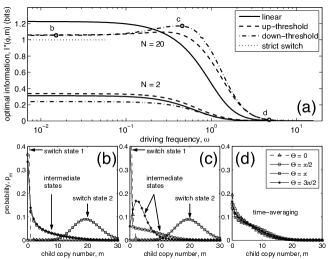
Figure 2: (a) At high copy number ($N=20$, top curves) the optimal information $I^{*}(\phi,m)$ exhibits a resonant driving frequency (point c) for up- (dashed) and down-threshold (dot-dashed) regulation, but not for linear (solid) regulation; at low copy number ($N=2$, bottom curves), there is no resonant frequency, and slowest ($\omega\rightarrow$ 0) is best. Panels (b-d) correspond to marked points in (a) and show the optimal child distribution for down-threshold regulation at phases $\Theta\equiv\omega t-\theta=0$, $\pi/2$, $\pi$, and $3\pi/2$ [legend in (d) applies to (b-d)]: (b) slow driving produces switch-like behavior, with long-lived high- ($\Theta=0$) and low-copy number ($\Theta=\pi$) states and brief intermediates ($\Theta=\pi/2,3\pi/2$) in between; (c) moderate driving produces switch-like behavior with distinguishable intermediates, transmitting the most information; and (d) fast driving time-averages the parent, and thus the child, distribution.

The above analytic approximations offer guidance during a full numerical optimization of $I(\phi,m)$ via the spectral method. As suggested by Eqn. 13, numerical optimization confirms that $I(\phi,m)$ increases when (i) the amplitude of the driving oscillation is maximal ($\alpha=g$) and (ii) the dynamic range is maximal ($q_{0}=0$ and $c\rightarrow\infty$ or $\Delta\rightarrow\infty$). The slope $c$ or discontinuity $\Delta$, however, is constrained by the average copy number of the child $\mu_{0}$ (Eqn. 11). Therefore for a fixed driving frequency and fixed total average copy number $N=\langle{n}\rangle+\langle{m}\rangle=g+\mu_{0}$, we optimize over the single parameter $g$ by setting $\alpha=g$, $q_{0}=0$, and $c=\mu_{0}/g=(N-g)/g$ or $\Delta=\mu_{0}/p^{0}_{\pm}=(N-g)/p_{\pm}^{0}$; additionally we set $\rho=1$ for equal decay rates (as is typical when decay rates are dominated by cell division Walczak et al. (2009)). For threshold regulation, an optimization over $g$ is done at each of a set of values of the (discrete) parameter $n_{0}$, and the global optimum is selected.

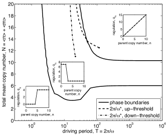
Figure 3: Phase diagram showing best optimal information $I^{*}(\phi,m)$ among linear, up-threshold, and down-threshold regulation in the space of driving period and copy number. Phases are separated by solid lines and marked by sample regulation functions (insets). Also shown is ($2\pi$ over) resonant frequency $\omega^{*}$ [see point c in Fig. 2(a)] as a function of copy number for both up- (dashed) and down-regulation (dot-dashed).

At low copy number, optimal information $I^{*}(\phi,m)$ behaves as one might expect from the small-oscillation limit (Eqn. 13): it decreases monotonically with frequency [Fig. 2(a), bottom curves]. At high copy number, $I^{*}(\phi,m)$ decreases monotonically with frequency for linear regulation but for threshold regulation exhibits a maximum at a resonant frequency [Fig. 2(a), top curves]. Careful examination of the child distribution at different phases [Fig. 2(b-d)] (or simply its mean, Sec. F) reveals the origin of this maximum as follows. As the parent oscillates about the threshold, the child distribution is switch-like, with two long-lived switch states centered at the threshold’s low and high rates, and brief intermediate states in between. At high copy number, the threshold rates are far apart (one is zero and the other is large), making the switch states well separated and transmitting (slightly more than, due to the intermediate states) the strict switch limit Walczak et al. (2009) of $I^{*}(\phi,m)\sim 1$ bit. For slow oscillations the intermediate states are symmetric [Fig. 2(b)], but for faster oscillations there is a lag in transitioning from one switch state to the other, making the intermediate states distinguishable [Fig. 2(c)], and transmitting more information about phase. Thus the resonant frequency $\omega^{*}$ balances the slowness required to avoid time-averaging [Fig. 2(d)] with the speed required for distinguishable intermediate states. As seen in Fig. 3, the onset of $\omega^{*}$ occurs above a critical copy number of $N^{*}\sim 10$.

Fig. 2(a) contains examples in which the most optimal regulation function is up-threshold (at low $N$), down-threshold (at high $N$ and high $\omega$) or linear (at high $N$ and low $\omega$). The phase diagram (Fig. 3) shows the results of this competition across a range of copy numbers $N$ and periods $T=2\pi/\omega$. Linear regulation is best when both $N$ and $T$ are large, ultimately surpassing threshold regulation’s limit of $\sim$$1$ bit. Down-threshold regulation is best at values of $T$ near $2\pi/\omega^{*}$ because its intermediate states are more distinguishable (i.e. have a larger Jensen-Shannon divergence) than those of a similarly parameterized up-threshold. Up-threshold regulation is best at low $N$ due to its tendency, as discussed above (Eqn. 14) and in Walczak et al. (2009), to require fewer proteins to match the transmission across a similarly parameterized down-threshold.

The low-pass behavior revealed in Eqns. 9 and 13 is consistent with our intuition from measuring static quantities in the presence of intrinsic noise Berg and Purcell (1977): the longer we wait, the more accurate is our estimate. However, in the presence of oscillatory driving, we find that threshold regulation can lead to an information-optimal frequency, and waiting longer is not necessarily the optimal strategy. Further, we have shown that, at a fixed allowed copy number and allowed integration time, one may find that a different regulation strategy (linear, threshold up-regulation, or threshold down-regulation) is optimal for responding to oscillatory driving. Absent from this analysis are intriguing questions such as whether the diversity of other network topologies observed in nature — including cascades and feedback circuits — are consistent with these observations. We anticipate the spectral method will continue to be useful in addressing these challenges.

Appendix A The parent distribution is a Poisson with oscillating mean

In this study we model two transcription factors — the ‘parent’ with copy number $n$ and the ‘child’ with copy number $m$ — each undergoing a birth-death process, with the parent’s birth rate an oscillatory function of time $f(t)=g+\alpha\cos\omega t$ and the child’s birth rate an arbitrary function $q_{n}$ of the parent copy number. The master equation,

$$\dot{p}_{nm} = f(t)p_{n-1,m}-f(t)p_{nm}$$ (15)

$$+(n+1)p_{n+1,m}-np_{nm}$$

$$+\rho[q_{n}p_{n,m-1}-q_{n}p_{nm}$$

$$+(m+1)p_{n,m+1}-mp_{nm}],$$

describes the time evolution of the joint probability of observing $n$ and $m$ copies of the parent and child, respectively. Here time is normalized via the parent decay rate (in these units $\rho$ is the child decay rate).

The equation for the parent distribution $p_{n}(t)$ is obtained by summing the master equation over $m$:

$$\dot{p}_{n} = f(t)p_{n-1}-f(t)p_{n}$$ (16)

$$+(n+1)p_{n+1}-np_{n}.$$

Since the parent is not regulated, Eqn. 16 simply describes a one-dimensional birth-death process with time-dependent birth rate $f(t)$. The solution can be found, regardless of the form of $f(t)$, using either (i) the method of characteristics, or (ii) the spectral method; for completeness we present both.

A.1 Method of characteristics

We begin the solution of Eqn. 16 by defining the generating function $G(x,t)=\sum_{n}p_{n}(t)x^{n}$ van Kampen (1992) over complex variable $x$ (writing $x=e^{ik}$ makes clear that the generating function is the Fourier transform in copy number). The utility of the generating function is that by summing Eqn. 16, which describes an infinite set of ordinary differential equations in $p_{n}$, over $n$ against $x^{n}$, it becomes a single partial differential equation in $G$,

$$\dot{G}=-(x-1)[\partial_{x}-f(t)]G.$$ (17)

The distribution is recovered by inverse transform, $p_{n}(t)=\partial^{n}_{x}\left[G(x,t)\right]_{x=0}/n!$.

We solve Eqn. 17 by the method of characteristics, in which we demand that $x$ and $t$ lie along a characteristic line $(x(s),t(s))$ parameterized by $s$, and we seek $G(s)$. Expressing Eqn. 17 as

$$(x-1)f(t)G=\frac{\partial G}{\partial t}+\frac{\partial G}{\partial x}(x-1),$$ (18)

it is clear that its consistency with the chain rule

$$\frac{dG}{ds}=\frac{\partial G}{\partial t}\frac{dt}{ds}+\frac{\partial G}{\partial x}\frac{dx}{ds}$$ (19)

requires

$$\frac{dt}{ds}=1 \Rightarrow t-t_{0}=s-s_{0},$$ (20)

$$\frac{dx}{ds}=x-1 \Rightarrow y=y_{0}e^{s-s_{0}}=y_{0}e^{t-t_{0}},\qquad$$ (21)

$$\frac{dG}{ds}=(x-1)f(t)G \Rightarrow \frac{dG}{dt}=y_{0}e^{t-t_{0}}f(t)G,$$ (22)

where $y\equiv x-1$, the last step of Eqn. 21 uses Eqn. 20, and the last step of Eqn. 22 uses Eqns. 20 and 21. We integrate Eqn. 22,

$$G(y,t)=G_{0}\exp\left[y_{0}e^{-t_{0}}\int_{t_{0}}^{t}dt^{\prime}\,e^{t^{\prime}}f(t^{\prime})\right],$$ (23)

and recognize that the initial condition $G_{0}$ is an arbitrary function of $y_{0}$; we may therefore expand as $G_{0}=\sum_{j}c_{j}y_{0}^{j}$ for some $c_{j}$. Inserting the characteristic equation $y_{0}=ye^{-(t-t_{0})}$ (Eqn. 21), Eqn. 23 becomes

$$G(y,t)=\sum_{j}c_{j}y^{j}e^{-j(t-t_{0})}e^{\nu(t)y}\rightarrow c_{0}e^{\nu(t)y},$$ (24)

where

$$\nu(t)\equiv e^{-t}\int_{t_{0}}^{t}dt^{\prime}\,e^{t^{\prime}}f(t^{\prime}),$$ (25)

and the last step in Eqn. 24 takes $t_{0}\rightarrow-\infty$ to give the post-transient behavior, upon which only the $j=0$ mode survives. Inverse transforming we find

$$p_{n}(t)=\frac{1}{n!}\partial^{n}_{x}\left[c_{0}e^{\nu(t)(x-1)}\right]_{0}=e^{-\nu(t)}\frac{\nu(t)^{n}}{n!}$$ (26)

(where $c_{0}=1$ by normalization), a Poisson distribution with time-dependent mean $\nu(t)$.

For oscillatory driving $f(t)=g+\alpha\cos\omega t$, the mean evaluates to

$$\nu(t) = g+\frac{\alpha}{1+\omega^{2}}\left(\cos\omega t+\omega\sin\omega t\right)$$ (27)

$$= \nu_{0}+2|\nu_{1}|\cos(\omega t-\gamma),$$ (28)

where $\nu_{0}=g$, $2|\nu_{1}|=\alpha/\sqrt{1+\omega^{2}}$, and $\gamma=\tan^{-1}\omega$. Eqn. 28 shows that the parent oscillates about the same point and with the same frequency as the driving birth rate, but that the oscillation is damped and phase-shifted at high frequency.

A.2 Spectral method

Eqn. 16 can also be solved using the spectral method Walczak et al. (2009); Mugler et al. (2009). Again we employ the generating function, this time expanding in a state space $|{n}\rangle{}$ indexed by copy number $n$: $|{G(t)}\rangle{}=\sum_{n}p_{n}(t)|{n}\rangle{}$. (Projecting onto the position space $\langle{x}|$ recovers the previous form with $\langle x|G(t)\rangle=G(x,t)$ and $\langle x|n\rangle=x^{n}$.) Summing Eqn. 16 against $|{n}\rangle{}$ gives

$$|{\dot{G}}\rangle{}=-(\hat{a}^{+}-1)[\hat{a}^{-}-f(t)]|{G}\rangle{}=-\hat{b}^{+}\hat{b}^{-}(t)|{G}\rangle{},$$ (29)

where the operators $\hat{a}^{+}$ and $\hat{a}^{-}$ raise and lower copy number, respectively, i.e. $\hat{a}^{+}|{n}\rangle{}=|{n+1}\rangle{}$ and $\hat{a}^{-}|{n}\rangle{}=n|{n-1}\rangle{}$ Doi (1976); Zel’Dovich and Ovchinnikov (1978); Peliti (1986); Mattis and Glasser (1998), and we define $\hat{b}^{+}\equiv\hat{a}^{+}-1$ and $\hat{b}^{-}(t)\equiv\hat{a}^{-}-f(t)$. (Note $\hat{a}^{+}\leftrightarrow x$ and $\hat{a}^{-}\leftrightarrow\partial_{x}$, as is clear from Eqns. 29 and 17.)

The spectral method exploits the linearity of the master equation by expanding $|{G}\rangle{}$ in the eigenfunctions $|{j}\rangle{}$ of a birth-death process Walczak et al. (2009); Mugler et al. (2009). Since here the birth rate $f(t)$ is time-dependent, we expand as

$$|{G}\rangle{}=\sum_{j}c_{j}|{j(t)}\rangle{}$$ (30)

where the time-dependent functions $\langle x|j(t)\rangle=(x-1)^{j}e^{\nu(t)(x-1)}$ are parameterized by the (as yet unknown) function $\nu(t)$. Noting that $\partial_{t}\langle x|j\rangle=\dot{\nu}\langle x|j+1\rangle$, the left-hand side of Eqn. 29 becomes $|{\dot{G}}\rangle{}=\sum_{j}\left[\dot{c}_{j}|{j}\rangle{}+\dot{\nu}c_{j}|{j+1}\rangle{}\right]$. Defining $\bar{b}^{-}(t)\equiv\hat{a}^{-}-\nu(t)=\hat{b}^{-}+f(t)-\nu(t)$ such that the $|{j(t)}\rangle{}$ are the eigenstates of $\hat{b}^{+}\bar{b}^{-}$, i.e.

$$\hat{b}^{+}\bar{b}^{-}|{j(t)}\rangle{}=j|{j(t)}\rangle{}$$ (31)

($\hat{b}^{+}$ and $\bar{b}^{-}$ raise and lower $|{j}\rangle{}$ as $\hat{a}^{+}$ and $\hat{a}^{-}$ do $|{n}\rangle{}$, respectively), the right-hand side of Eqn. 29 becomes $\sum_{j}c_{j}\left\{-j|{j}\rangle{}+[f(t)-\nu(t)]|{j+1}\rangle{}\right\}$. Therefore projecting $\langle{j^{\prime}}|$ onto Eqn. 29 gives the following equation for the expansion coefficients $c_{j}$:

$$\dot{c}_{j}+\dot{\nu}c_{j-1}=-jc_{j}+[f(t)-\nu(t)]c_{j-1}.$$ (32)

The dynamics are trivial if $\dot{\nu}=-\nu+f(t)$, an equation whose solution is Eqn. 25. In this case Eqn. 32 is solved by $c_{j}=e^{-j(t-t_{0})}$, which becomes $\delta_{j0}$ as $t_{0}\rightarrow-\infty$ (for post-transient behavior). The probability distribution is obtained by inverse transform,

$$p_{n}(t)=\langle n|G\rangle=\sum_{j}c_{j}\langle n|j\rangle=\langle n|0\rangle=e^{-\nu(t)}\frac{\nu(t)^{n}}{n!},$$ (33)

where the last step uses the fact the the zero mode $\langle n|0\rangle$ is a Poisson distribution at the eigenfunction parameter (or gauge) $\nu(t)$ Walczak et al. (2009); Mugler et al. (2009). Eqn. 33 reproduces the result from the method of characteristics, Eqn. 26.

Appendix B Fourier transform of the parent distribution

The Fourier coefficients of a Poisson distribution with oscillating mean are here found analytically in terms of spectral modes. We begin by representing the distribution as

$$p(n|\phi)=e^{-\nu(\phi)}\frac{\nu(\phi)^{n}}{n!}=\frac{1}{n!}\partial^{n}_{x}\left[e^{\nu(\phi)(x-1)}\right]_{0},$$ (34)

where $\phi=\omega t$, and

$$\nu(\phi)=\nu_{0}+2|\nu_{1}|\cos(\phi-\gamma)=\nu_{0}+|\nu_{1}|\sum_{\pm}e^{\pm i(\phi-\gamma)}.$$ (35)

The Fourier transform will have support only at harmonics $z$ of the driving frequency, i.e.

$$p_{n}^{z} = \int_{0}^{2\pi}\frac{d\phi}{2\pi}e^{iz\phi}p(n|\phi)$$ (37)

$$= \int_{0}^{2\pi}\frac{d\phi}{2\pi}e^{iz\phi}\frac{1}{n!}\partial^{n}_{x}\Biggl{[}e^{\nu_{0}(x-1)}$$

$$\left.\times\exp\left\{(x-1)|\nu_{1}|\sum_{\pm}e^{\pm i(\phi-\gamma)}\right\}\right]_{0}.$$

Expanding the exponential and then invoking the binomial expansion on the $\pm$ sum,

$$p_{n}^{z} = \int_{0}^{2\pi}\frac{d\phi}{2\pi}e^{iz\phi}\frac{1}{n!}\partial^{n}_{x}\Biggl{[}e^{\nu_{0}(x-1)}$$ (38)

$$\times\sum_{j=0}^{\infty}\frac{(x-1)^{j}|\nu_{1}|^{j}}{j!}$$

$$\left.\times\sum_{\ell=0}^{j}\frac{j!}{\ell!(j-\ell)!}e^{i(\phi-\gamma)(j-\ell)}e^{-i(\phi-\gamma)\ell}\right]_{0}.$$

Reordering terms,

$$p_{n}^{z} = \sum_{j=0}^{\infty}|\nu_{1}|^{j}$$ (39)

$$\times\frac{1}{n!}\partial^{n}_{x}\left[e^{\nu_{0}(x-1)}(x-1)^{j}\right]_{0}$$

$$\times\sum_{\ell=0}^{j}\frac{e^{-i(j-2\ell)\gamma}}{\ell!(j-\ell)!}$$

$$\times\int_{0}^{2\pi}\frac{d\phi}{2\pi}e^{i(j-2\ell+z)\phi}.$$

The second line in Eqn. 39 is the derivative representation of the spectral mode $\langle n|j\rangle$ Walczak et al. (2009); Mugler et al. (2009), with parameter (or gauge) $\nu_{0}$. The fourth line in Eqn. 39 evaluates to $\delta_{0,j-2\ell+z}$, which collapses the $\ell$ sum nonvanishingly provided $z+j$ is an even number from $0$ to $2j$, or $z\in\{-j,-j+2,\dots,j-2,j\}$. This criterion can be equivalently be expressed as a condition on $j$ in terms of $z$: $j\in\{|z|,|z|+2,|z|+4,\dots,\infty\}\equiv\Omega$, making Eqn. 39

$$p_{n}^{z}=e^{iz\gamma}\sum_{j\in\Omega}\frac{|\nu_{1}|^{j}\langle n|j\rangle}{[(j+z)/2]![(j-z)/2]!}$$ (40)

Defining $j^{\prime}\equiv(j-|z|)/2$ allows the sum to run from $0$ to $\infty$ and yields the simplification $[(j+z)/2]![(j-z)/2]!=j^{\prime}!(j^{\prime}+|z|)!$ for all integer $z$, making Eqn. 40

$$p_{n}^{z}=e^{iz\gamma}\sum_{j^{\prime}=0}^{\infty}\frac{|\nu_{1}|^{2j^{\prime}+|z|}}{j^{\prime}!(j^{\prime}+|z|)!}\left\langle n\big{|}2j^{\prime}+|z|\right\rangle,$$ (41)

as in Eqn. 6.

Appendix C Expansion in the small-information limit

Here we explicitly expand the log in Eqn. 7 and show that the first two terms contribute to the leading-order behavior in $p_{n}^{z}$. Eqn. 7 reads

$$I(\phi,n)=\sum_{n,z}p_{n}^{z}\int_{0}^{2\pi}\frac{d\phi}{2\pi}e^{-iz\phi}\log\left(1+\sum_{z^{\prime}\neq 0}\frac{p_{n}^{z^{\prime}}}{p_{n}^{0}}e^{-iz^{\prime}\phi}\right).$$ (42)

Since, for small $|\nu_{1}|$, Eqn. 41 is dominated by the $j^{\prime}=0$ term, i.e.

$$p_{n}^{z}\approx e^{iz\gamma}\frac{|\nu_{1}|^{|z|}}{|z|!}\left\langle n\big{|}|z|\right\rangle,$$ (43)

which is small for $z\neq 0$, we expand the log:

$$I = \sum_{n,z}p_{n}^{z}\int_{0}^{2\pi}\frac{d\phi}{2\pi}e^{-iz\phi}$$ (44)

$$\times\sum_{\ell=1}^{\infty}\frac{(-1)^{\ell+1}}{\ell}\left(\sum_{z^{\prime}\neq 0}\frac{p_{n}^{z^{\prime}}}{p_{n}^{0}}e^{-iz^{\prime}\omega t}\right)^{\ell},$$

or, explicitly writing out the $\ell$ sums,

$$I = \sum_{n,z}p_{n}^{z}\int_{0}^{2\pi}\frac{d\phi}{2\pi}e^{-iz\phi}\sum_{\ell=1}^{\infty}\frac{(-1)^{\ell+1}}{\ell(p_{n}^{0})^{\ell}}$$ (45)

$$\times\sum_{z_{1}\neq 0}p_{n}^{z_{1}}e^{-iz_{1}\phi}\sum_{z_{2}\neq 0}p_{n}^{z_{2}}e^{-iz_{2}\phi}\dots$$

$$\times\sum_{z_{\ell}\neq 0}p_{n}^{z_{\ell}}e^{-iz_{\ell}\phi}.$$

Reordering terms as

$$I = \sum_{\ell=1}^{\infty}\frac{(-1)^{\ell+1}}{\ell}\sum_{n}\frac{1}{(p_{n}^{0})^{\ell}}$$ (46)

$$\times\sum_{z_{1}\neq 0}p_{n}^{z_{1}}\sum_{z_{2}\neq 0}p_{n}^{z_{2}}\dots\sum_{z_{\ell}\neq 0}p_{n}^{z_{\ell}}\sum_{z}p_{n}^{z}$$

$$\times\int_{0}^{2\pi}\frac{d\phi}{2\pi}e^{-i(z+z_{1}+z_{2}+\dots+z_{\ell})\phi},$$

and employing $\int_{0}^{2\pi}d\phi\,e^{is\phi}=2\pi\delta_{s0}$ for integer $s$ allows us to collapse the $z$ sum,

$$I = \sum_{\ell=1}^{\infty}\frac{(-1)^{\ell+1}}{\ell}\sum_{n}\frac{1}{(p_{n}^{0})^{\ell}}$$ (47)

$$\times\sum_{z_{1}\neq 0}p_{n}^{z_{1}}\sum_{z_{2}\neq 0}p_{n}^{z_{2}}\dots\sum_{z_{\ell}\neq 0}p_{n}^{z_{\ell}}$$

$$\times p_{n}^{-(z_{1}+z_{2}+\dots+z_{\ell})}.$$

Now, since $p_{n}^{z}\propto|\nu_{1}|^{|z|}$ for small $|\nu_{1}|$ (Eqn. 43), $I(\phi,n)$ will be dominated by the leading-order term in $|z|$. Writing out the first few terms in Eqn. 47 explicitly,

$$I = \sum_{n}\frac{1}{p_{n}^{0}}\sum_{z\neq 0}p_{n}^{z}p_{n}^{-z}$$ (48)

$$-\frac{1}{2}\sum_{n}\frac{1}{(p_{n}^{0})^{2}}\sum_{x\neq 0}p_{n}^{x}\sum_{y\neq 0}p_{n}^{y}p_{n}^{-(x+y)}$$

$$+\frac{1}{3}\sum_{n}\frac{1}{(p_{n}^{0})^{3}}\sum_{u\neq 0}p_{n}^{u}\sum_{v\neq 0}p_{n}^{v}\sum_{w\neq 0}p_{n}^{w}p_{n}^{-(u+v+w)}$$

$$+\dots,$$

we see that the leading-order term is proportional to $p_{n}^{1}p_{n}^{-1}=|p_{n}^{1}|^{2}$ and has contributions from both the first ($z=\pm 1$) and the second ($(x,y)=(\pm 1,\mp 1)$) term in the log expansion. To leading order, then,

$$I\approx\left[1+1-\frac{1}{2}(1+1)\right]\sum_{n}\frac{|p_{n}^{1}|^{2}}{p_{n}^{0}}=\sum_{n}\frac{|p_{n}^{1}|^{2}}{p_{n}^{0}},$$ (49)

as in Eqn. 8.

Appendix D Useful properties of the spectral modes

D.1 Relating spectral modes to distribution moments

The eigenfunctions of a birth-death process, or ‘spectral modes,’ define a complete basis in which any distribution $p_{n}$ can be expanded, i.e.

$$p_{n}=\sum_{j}c_{j}\langle n|j\rangle$$ (50)

(where the expansion coefficients are computed by inverse transform: $c_{j}=\sum_{n}p_{n}\langle j|n\rangle$). The goal of this section is to relate the spectral modes to the distribution moments $\langle{n^{\ell}}\rangle=\sum_{n}n^{\ell}p_{n}$.

The $\ell$th moment is $\langle{n^{\ell}}\rangle=\sum_{j}c_{j}\eta^{\ell}_{j}$, where

$$\eta^{\ell}_{j}\equiv\sum_{n}n^{\ell}\langle n|j\rangle=\sum_{n}n^{\ell}\oint\frac{dx}{2\pi i}\frac{(x-1)^{j}e^{g(x-1)}}{x^{n+1}}.$$ (51)

The last step uses the integral representation of $\langle n|j\rangle$ over complex variable $x$ Mugler et al. (2009). Isolating the $n$-dependence, we may write

$$\eta^{\ell}_{j}=\oint\frac{dx}{2\pi i}(x-1)^{j}e^{g(x-1)}\frac{1}{x}S_{\ell},$$ (52)

where for $w\equiv 1/x$,

$$S_{\ell}\equiv\sum_{n}n^{\ell}w^{n}=\sum_{n}\left(w\partial_{w}\right)^{\ell}w^{n}=\left(w\partial_{w}\right)^{\ell}\frac{1}{1-w},$$ (53)

and the last step sums the geometric series. Computing the first few derivatives in Eqn. 53 reveals the pattern

$$S_{\ell}=\frac{\sum_{u=0}^{\ell}A_{\ell u}w^{\ell-u}}{(1-w)^{\ell+1}}=\frac{\sum_{u=0}^{\ell}A_{\ell u}x^{u+1}}{(x-1)^{\ell+1}},$$ (54)

in terms of the Eulerian numbers

$$A_{\ell u}=\sum_{v=0}^{u}(-1)^{v}\begin{pmatrix}\ell+1\\ v\end{pmatrix}(u+1-v)^{\ell},$$ (55)

making Eqn. 52

$$\eta^{\ell}_{j}=\sum_{u=0}^{\ell}A_{\ell u}\oint\frac{dx}{2\pi i}\frac{x^{u}}{(x-1)^{\ell-j+1}e^{-g(x-1)}}.$$ (56)

The integral is recognized as a representation of the conjugate mode $\langle j^{\prime}|n^{\prime}\rangle$ with $j^{\prime}=\ell-j\geq 0$, $n^{\prime}=u\geq 0$, and parameter (or gauge) $-g$ Mugler et al. (2009). Modes and conjugate modes can be evaluated either recursively using selection rules or explicitly using Cauchy’s theorem Mugler et al. (2009). Conjugate modes $\langle j^{\prime}|n^{\prime}\rangle$ with gauge $g^{\prime}$ are $j^{\prime}$th order polynomials in $n^{\prime}$; the first few are

$$\langle j^{\prime}=0|n^{\prime}\rangle = 1,$$ (57)

$$\langle j^{\prime}=1|n^{\prime}\rangle = n^{\prime}-g^{\prime},$$ (58)

$$\langle j^{\prime}=2|n^{\prime}\rangle = \frac{1}{2}n^{\prime 2}-\left(g^{\prime}+\frac{1}{2}\right)n^{\prime}+\frac{g^{\prime 2}}{2}.$$ (59)

Thus the first few $\eta^{\ell}_{j}$ are (Eqn. 56)

$$\sum_{n}\langle n|j\rangle = \eta^{\ell=0}_{j}=\delta_{j0},$$ (60)

$$\sum_{n}n\langle n|j\rangle = \eta^{\ell=1}_{j}=g\delta_{j0}+\delta_{j1},$$ (61)

$$\sum_{n}n^{2}\langle n|j\rangle = \eta^{\ell=2}_{j}$$ (62)

$$= g(g+1)\delta_{j0}+(2g+1)\delta_{j1}+2\delta_{j2},\qquad$$

and in general the $\ell$th moment is calculated $\langle{n^{\ell}}\rangle=\sum_{j}c_{j}\eta^{\ell}_{j}$.

Eqns. 60 and 61 are useful in describing the mean properties of a child species regulated by the linear function $q_{n}=q_{0}+cn$. As described in Eqn. 11, the mean of the child distribution oscillates about the point

$$\mu_{0}=\sum_{n}q_{n}p_{n}^{0}=\sum_{n}(q_{0}+cn)\sum_{j}\frac{|\nu_{1}|^{2j}}{(j!)^{2}}\langle n|2j\rangle,$$ (63)

where the last step uses the Fourier transform of the parent distribution, Eqn. 41. Evaluating the $n$ sum using Eqns. 60 and 61 gives

$$\mu_{0} = \sum_{j}\frac{|\nu_{1}|^{2j}}{(j!)^{2}}\left[q_{0}\delta_{2j,0}+c(g\delta_{2j,0}+\delta_{2j,1})\right]$$ (64)

$$= q_{0}+cg,$$ (65)

(since only the first and second Kronecker delta have support for integer $j$), as in Eqn. 11 (top).

Similarly, as described in Eqn. 12, the amplitude of the oscillation of the child mean is

$$|\mu_{1}| = \frac{\sum_{n}q_{n}|p_{n}^{1}|}{\sqrt{1+(\omega/\rho)^{2}}}=\frac{1}{\sqrt{1+(\omega/\rho)^{2}}}$$ (66)

$$\times\sum_{n}(q_{0}+cn)\sum_{j}\frac{|\nu_{1}|^{2j+1}}{j!(j+1)!}\langle n|2j+1\rangle.\qquad$$

Again employing Eqns. 60 and 61,

$$|\mu_{1}| = \frac{1}{\sqrt{1+(\omega/\rho)^{2}}}\sum_{j}\frac{|\nu_{1}|^{2j+1}}{j!(j+1)!}$$ (67)

$$\times\left[q_{0}\delta_{2j+1,0}+c(g\delta_{2j+1,0}+\delta_{2j+1,1})\right]$$

$$= \frac{c|\nu_{1}|}{\sqrt{1+(\omega/\rho)^{2}}}$$ (68)

(since only the last Kronecker delta has support for integer $j$), as in Eqn. 12 (top).

D.2 Sums of differences

The zero mode (i.e. the steady-state solution) of the birth-death process with birth rate (or gauge) $g$ is the Poisson distribution,

$$\langle n|j=0\rangle=e^{-g}\frac{g^{n}}{n!}$$ (69)

(recall that time is normalized by the decay rate). Each higher mode is related to the previous mode by discrete derivative Mugler et al. (2009):

$$\langle n|j+1\rangle=-\partial_{n}^{-}\langle n|j\rangle=\langle n-1|j\rangle-\langle n|j\rangle.$$ (70)

This property is especially useful when performing a finite sum, since only the boundary terms survive:

$$\sum_{n=a}^{b}\langle n|j+1\rangle=\langle a-1|j\rangle-\langle b|j\rangle.$$ (71)

We make use of Eqn. 71 in arriving at Eqns. 11 (bottom) and 12 (bottom), describing the mean properties of a child species regulated by the threshold function $q_{n}=q_{0}+\Delta\chi(n\in\Omega_{\pm})$. Here $\chi$ is a characteristic function equal to $1$ when $n$ is in the set $\Omega_{+}=\{n>n_{0}\}=\{n_{0}+1,\dots,\infty\}$ (for up-regulation) or $\Omega_{-}=\{n\leq n_{0}\}=\{0,\dots,n_{0}\}$ (for down-regulation), and $0$ otherwise. In Eqn. 11 (bottom),

$$\mu_{0} = \sum_{n}q_{n}p_{n}^{0}$$ (72)

$$= \sum_{n}[q_{0}+\Delta\chi(n\in\Omega_{\pm})]\sum_{j}\frac{|\nu_{1}|^{2j}}{(j!)^{2}}\langle n|2j\rangle,$$ (73)

$$= q_{0}+\Delta\sum_{j}\frac{|\nu_{1}|^{2j}}{(j!)^{2}}\sum_{n\in\Omega_{\pm}}\langle n|2j\rangle,$$ (74)

where the $q_{0}$ term collapses as in Eqn. 65. The $j=0$ term reduces explicitly to $\Delta\pi_{\pm}$, where $\pi_{\pm}\equiv\sum_{n\in\Omega_{\pm}}\langle n|0\rangle$. For any $j^{\prime}>0$ we may employ Eqn. 71,

$$\sum_{n=n_{0}+1}^{\infty}\langle n|j^{\prime}\rangle = \langle n_{0}|j^{\prime}-1\rangle,$$ (75)

$$\sum_{n=0}^{n_{0}}\langle n|j^{\prime}\rangle = -\langle n_{0}|j^{\prime}-1\rangle,$$ (76)

(since the boundary terms at $n=-1$ and $\infty$ vanish), making Eqn. 74

$$\mu_{0}=q_{0}+\Delta\left[\pi_{\pm}\pm\sum_{j>0}\frac{|\nu_{1}|^{2j}}{(j!)^{2}}\langle n_{0}|2j-1\rangle\right],$$ (77)

as in Eqn. 11 (bottom). In Eqn. 12 (bottom),

$$|\mu_{1}| = \frac{\sum_{n}q_{n}|p_{n}^{1}|}{\sqrt{1+(\omega/\rho)^{2}}}$$ (79)

$$= \frac{1}{\sqrt{1+(\omega/\rho)^{2}}}\sum_{n}[q_{0}+\Delta\chi(n\in\Omega_{\pm})]$$

$$\times\sum_{j}\frac{|\nu_{1}|^{2j+1}}{j!(j+1)!}\langle n|2j+1\rangle$$

$$= \frac{\Delta}{\sqrt{1+(\omega/\rho)^{2}}}\sum_{j}\frac{|\nu_{1}|^{2j+1}}{j!(j+1)!}\sum_{n\in\Omega_{\pm}}\langle n|2j+1\rangle,\qquad$$ (80)

where the $q_{0}$ term vanishes as in Eqn. 68. Again using Eqns. 75 and 76,

$$|\mu_{1}|=\Delta\sum_{j}\frac{|\nu_{1}|^{2j+1}}{j!(j+1)!}\langle n_{0}|2j\rangle,$$ (81)

as in Eqn. 12 (bottom), where for the down-threshold the negative sign is absorbed into the definition $\mu(t)\approx\mu_{0}\pm 2|\mu_{1}|\cos(\omega t-\theta)$.

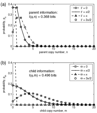
Figure 4: The child can tell better time than the parent. Parent (a) and child (b) distributions are plotted at phases $\Gamma\equiv\omega t-\gamma$ and $\Theta\equiv\omega t-\theta$ equal to $0$, $\pi/2$, $\pi$, and $3\pi/2$, where $\gamma$ and $\theta$ are the phase shifts of the parent and child means, respectively. Regulation is linear and steep (slope $c=3$); other parameters are $g=\alpha=\rho=1$ and $\omega=q_{0}=0$.

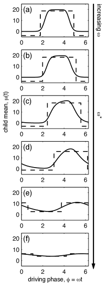
Figure 5: Information-optimal child distribution mean $\mu(t)=\sum_{m}p_{m}(t)$ (solid) as a function of phase $\phi=\omega t$ for threshold down-regulation and fixed copy number $N=20$ and driving frequency $\omega=$ (a) $0.10$, (b) $0.21$, (c) $0.46$, (d) $0.91$, (e) $1.91$, and (f) $3.98$. Panel (c) corresponds to resonant frequency $\omega^{*}$ at which optimal information $I^{*}(\phi,m)$ is greatest. For comparison, dashed lines show square waves centered at $\mu_{0}$ with amplitude $2|\mu_{1}|$ and phase shift $\theta={\rm phase}(\mu_{1})$.

D.3 Differentiation with respect to gauge

The derivative of spectral mode $\langle n|j\rangle$ with respect to its gauge $g$ is

$$\partial_{g}\langle n|j\rangle=\langle n|j+1\rangle,$$ (82)

a property that can be seen most readily from the integral representation of $\langle n|j\rangle$ (Eqn. 51). This property is useful in expediting derivative calculations, for example Eqn. 14, which uses

$$\partial_{g}\langle n_{0}|0\rangle = \langle n_{0}|1\rangle=\langle n_{0}|0\rangle\left(\frac{n_{0}}{g}-1\right),$$ (83)

$$\partial_{g}\pi_{\pm} = \partial_{g}\sum_{n\in\Omega_{\pm}}\langle n|0\rangle=\sum_{n\in\Omega_{\pm}}\langle n|1\rangle=\pm\langle n_{0}|0\rangle,\qquad$$ (84)

where the last step in Eqn. 83 uses Eqn. 70, and the last step in Eqn. 84 uses Eqns. 75 and 76.

Appendix E The child can tell better time than the parent

Although the master equation (Eqn. 15) is Markovian in time (i.e. the probability of making a transition at time $t$ is independent of previous transitions), it is not explicitly Markovian in the variables $t$, $n$, and $m$: $p(m|t)\neq\sum_{n}p(m|n)p(n|t)$. As such, information transmission is not bound by the data-processing inequality Cover and Thomas (1991), and it is possible for the child to transmit more information than the parent about the driving phase, $I(\phi,m)>I(\phi,n)$. This possibility is explicitly apparent in the small-oscillation limit with linear regulation, Eqn. 13 (top),

$$I(\phi,m)=\frac{gc^{2}}{(q_{0}+cg)[1+(\omega/\rho)^{2}]}I(\phi,n),$$ (85)

for example if $\omega\rightarrow 0$, $q_{0}=0$, and $c>1$. However, because these are the very parameter settings that strain the approximations under which Eqn. 85 is derived (i.e. weak or fast oscillation and near-constant regulation), it is useful to also demonstrate numerically via the spectral method a case in which $I(\phi,m)>I(\phi,n)$. Fig. 4 shows clearly that if the regulation is sufficiently steep, the oscillation is sufficiently amplified and the child tells better time than the parent does, i.e. $I(\phi,m)>I(\phi,n)$.

Appendix F Threshold regulation can exhibit a resonant frequency

When the regulation function is a threshold and the total copy number $N$ is sufficiently high, the optimal information $I^{*}(\phi,m)$ exhibits a maximum at a resonant frequency $\omega^{*}$. In Fig. 2 it is shown that $\omega^{*}$ is the frequency at which the driving oscillation is slow enough for the output to be switch-like (and avoid time-averaging), but fast enough for the brief states in between the switch states to be distinguishable from each other.

Fig. 5 here plots the mean $\mu(t)$ of the child distribution against phase for a range of driving frequencies. At low frequency [Fig. 5(a)], the output is switch-like, and $\mu(t)$ is well approximated by a square wave. At the resonant frequency [Fig. 5(c)], the output is still switch-like but no longer symmetric in time, the asymmetry arising from a lag in transitioning from one switch state to the other (the lag allows the transitions to be distinguished from each other, maximizing transmission of information about phase). At high frequency, [Fig. 5(f)] the driving is faster than the parent decay rate, and both parent and child distributions are time-averaged.

References

Berg and Purcell (1977)
H. C. Berg and
E. M. Purcell,
Biophys. J 20,
193 (1977).
Mettetal et al. (2008)
J. Mettetal,
D. Muzzey,
C. Gomez-Uribe,
and A. van
Oudenaarden, Science 319,
482 (2008).
Elowitz and Leibler (2000)
M. B. Elowitz and
S. Leibler,
Nature 403,
335 (2000).
Tostevin and ten Wolde (2009)
F. Tostevin and
P. R. ten Wolde,
Phys. Rev. Lett. 102,
218101 (2009).
Tănase-Nicola et al. (2006)
S. Tănase-Nicola,
P. B. Warren,
and P. R. ten
Wolde, Phys Rev Lett 97,
68102 (2006).
Tkacik et al. (2008)
G. Tkacik,
C. G. Callan,
and W. Bialek,
Proc Natl Acad Sci USA 105,
12265 (2008).
Bialek and Setayeshgar (2005)
W. Bialek and
S. Setayeshgar,
Proc Natl Acad Sci USA 102,
10040 (2005).
Walczak et al. (2009)
A. M. Walczak,
A. Mugler, and
C. H. Wiggins,
Proc Natl Acad Sci USA 106,
6529 (2009).
Mugler et al. (2009)
A. Mugler,
A. M. Walczak,
and C. H.
Wiggins, Phys. Rev. E
80, 41921 (2009).
Csikász-Nagy
et al. (2006)
A. Csikász-Nagy,
D. Battogtokh,
K. C. Chen,
B. Novák,
and J. J. Tyson,
Biophys. J 90,
4361 (2006).
Cookson et al. (2009)
N. Cookson,
L. Tsimring, and
J. Hasty,
FEBS letters (2009).
Shannon (1949)
C. E. Shannon,
Proc IRE 37,
10 (1949).
Cover and Thomas (1991)
T. M. Cover and
J. A. Thomas,
Elements of Information Theory
(New York, NY: John Wiley and Sons,
1991).
van Kampen (1992)
N. G. van Kampen,
Stochastic processes in physics and chemistry
(Amsterdam: North-Holland, 1992).
Doi (1976)
M. Doi,
Journal of Physics A: Mathematical and General
9, 1465 (1976).
Zel’Dovich and Ovchinnikov (1978)
Y. B. Zel’Dovich
and A. A.
Ovchinnikov, Soviet Journal of
Experimental and Theoretical Physics 47,
829 (1978).
Peliti (1986)
L. Peliti,
Journal of Physics A: Mathematical and General
19, L365 (1986).
Mattis and Glasser (1998)
D. C. Mattis and
M. L. Glasser,
Reviews of Modern Physics 70,
979 (1998).