Kramers escape driven by fractional Brownian motion

Abstract

We investigate the Kramers escape from a potential well of a test particle driven by fractional Gaussian noise with Hurst exponent $0<H<1$. From a numerical analysis we demonstrate the exponential distribution of escape times from the well and analyze in detail the dependence of the mean escape time as function of $H$ and the particle diffusivity $D$. We observe different behavior for the subdiffusive (antipersistent) and superdiffusive (persistent) domains. In particular we find that the escape becomes increasingly faster for decreasing values of $H$, consistent with previous findings on the first passage behavior. Approximate analytical calculations are shown to support the numerically observed dependencies.

I Introduction

Anomalous diffusion is characterized by a deviation from the classical linear time dependence $\langle x^{2}(t)\rangle\simeq t$ of the mean squared displacement. Such anomalies range from ultraslow transport $\langle x^{2}\rangle\simeq\log^{\beta}t$ as discovered in Sinai diffusion or in iterated maps sinai ; julia , up to cubic diffusion $\langle x(t)\rangle\simeq t^{3}$ in random walk processes with correlated jump lengths vincent1 or the relative coordinate of two particles encountered in turbulent Richardson flow richardson ; boffetta . Here we are interested in anomalous diffusion of the power-law type bouchaud ; report

$$\langle x^{2}(t)\rangle=2Dt^{2H},$$ (1)

where $H$ is the Hurst exponent and $D$ the generalized diffusion coefficient of dimension $[D]=\mathrm{cm}^{2}/\mathrm{sec}^{2H}$. Depending on the magnitude of $H$ we observe subdiffusion ($0<H<1/2$) or superdiffusion ($1/2<H<1$). The limits $H=1/2$ and $H=1$ correspond to ordinary Brownian diffusion or ballistic motion, respectively. For one-particle motion ballistic transport is the upper limit of spreading when the particle has a finite maximum velocity.

Anomalous diffusion of the power law form (1) is observed in a multitude of systems. In particular, subdiffusion was found for the motion of charge carriers in amorphous semiconductors scher ; pfister , the spreading of tracer molecules in subsurface hydrology scher_grl , diffusion on random site percolation clusters klemm as well as the motion of tracers in the crowded environment of biological cells bio or in reconstituted biological systems alabio , among many others. Examples for superdiffusion include active motion in biological cells caspi , tracer spreading in layered velocity fields matheron , turbulent rotating flows swinney , or in bulk mediated surface exchange stapf .

Apart from numerical approaches there exist two prominent analytical models for such anomalous diffusion: One is the continuous time random walk (CTRW) model scher ; klablushle in which each jump is characterized by a variable jump length and waiting time drawn from associated probability densities. CTRW theory includes (i) subdiffusion when the variance of jump lengths is finite but the waiting times have an infinite characteristic time; (ii) Lévy flights when the mean waiting time is finite but the jump length variance diverges; and (iii) Lévy walks in which waiting times and jump lengths are coupled, producing sub-ballistic superdiffusion with finite variance. The escape over a potential barrier for subdiffusion and Lévy flights was studied recently mekla ; levykramers ; imkeller ; ditlevsen .

The second model is fractional Brownian motion (FBM). It was originally described by Kolmogorov kolmogorov and reintroduced by Mandelbrot and van Ness mandelbrot . FBM is a self-similar Gaussian process with stationary increments Yaglom ; Qian . The FBM mean squared displacement follows Eq. (1), and the Hurst exponent $H$ of the fractional Gaussian noise varies in the full range $0<H<1$. Uncorrelated, regular Brownian motion corresponds to $H=1/2$. For $0<H<1/2$ the prefactor in the noise autocorrelation is negative, rendering the associated antipersistent process subdiffusive. That means that a step in one direction is likely followed by a step in the other direction. Conversely, in the case $1/2<H<1$ the motion is persistent, effecting sub-ballistic superdiffusion in which successive steps tend to point in the same direction. FBM is used to model a variety of processes including monomer diffusion in a polymer chain gleb , single file diffusion tobias , diffusion of biopolymers in the crowded environment inside biological cells guigas , long term storage capacity in reservoirs hurst , climate fluctuations palmer , econophysics mandelbrot1 , and teletraffic mikosch .

Despite its wide use FBM is not completely understood. Thus the general incorporation of non-trivial boundary conditions is unattained, in particular, the first passage behavior is solved analytically solely on a semi-infinite domain Molchan . Notably the method of images does not apply to solve boundary value problems for FBM. Similarly the associated fractional Langevin equation driven by fractional Gaussian noise was recently discovered to exhibit critical dynamical behavior stas .

Here we study the generalization for FBM of the Kramers escape from a potential well across a finite barrier, as illustrated in Fig. 1. This problem is relevant, for instance, for single file diffusion in external potentials eli , the dissociation dynamics of biopolymers from a bound state in FBM models for particle diffusion under molecular crowding conditions guigas or bulk chemical reactions of larger particles under superdense conditions. We note that a similar problem was treated for correlated Gaussian noise katja and for fractional Langevin equation motion in the case when the fluctuation dissipation theorem applies goychuk . We here study the important case of external fluctuations, that is, for systems which do not obey the fluctuation dissipation theorem klimontovich .

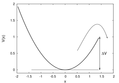
Figure 1: Harmonic potential $V(x)=x^{2}/2$ with cutoff at $x=\sqrt{2}$ used in the numerical analysis of the FBM Kramers escape. The potential barrier height is $\Delta V=1$. Dimensionless units.

In the regular Kramers theory kramers ; chandrasekhar ; risken for the escape of a Brownian particle across a potential barrier in the high barrier limit $\Delta V\gg k_{B}\theta$, where $k_{B}\theta$ denotes thermal energy, the probability density of the first escape from the well follows an exponential decay,

$$p(t)\simeq\exp\left(-\frac{t}{T}\right).$$ (2)

This corresponds to the relaxation mode of the lowest eigenvalue kramers ; chandrasekhar ; risken . In Eq. (2) the characteristic escape time $T$ is proportional to the Arrhenius factor of the barrier height $\Delta V$,

$$T\propto\exp\left(\frac{\Delta V}{k_{B}\theta}\right).$$ (3)

In what follows we demonstrate from simulations and analytical considerations that the exponential decay (2) is preserved in FBM processes due to the stationary nature of FBM, while the activation pattern (3) becomes explicitly dependent on the Hurst exponent. This $H$-dependence is different for the antipersistent and persistent cases. Remarkably slow diffusion leads to fast escape, that is, the lower the value of $H$ is chosen the faster the escape from the potential well becomes. This observation is consistent with the first passage behavior of FBM that is known analytically, and analysed numerically in the Appendix.

We first investigate FBM driven Kramers escape by numerical integration of the Langevin equation subject to fractional Gaussian noise in Sec. II. In particular, we analyze the distribution of escape times and the dependence of the mean escape time on the Hurst exponent $H$ and the noise strength $D$. In Sec. III we develop an approximate analytical approach to the barrier crossing for FBM, before drawing our conclusions in Sec. IV. In the Appendices we describe the numerical algorithms used to generate antipersistent and persistent FBM, and we validate in detail that these truthfully produce FBM. We also briefly discuss the consistency of our results for the case of a potential well, that is finite on both sides.

II Numerical analysis

In this Section we set up the Langevin description of FBM for external Gaussian noise and present extensive simulations results for the barrier crossing behavior.

II.1 Langevin equation with fractional Gaussian noise

We employ the overdamped Langevin equation for the position variable $x(t)$ in the presence of an external potential $V(x)$,

$$\frac{dx(t)}{dt}=-\frac{1}{m\gamma}\frac{dV(x)}{dx}+\sqrt{D}\xi_{H}(t),$$ (4)

where $m$ is the particle mass, $\gamma$ the friction constant, $\xi_{H}(t)$ is the fractional Gaussian noise, and $D$ is its intensity. The chosen initial condition is $x(0)=0$. To study the activated escape from a potential well, in what follows we use an harmonic potential of the form

$$V(x)=\left\{\begin{array}[]{ll}\frac{a}{2}x^{2},&-\infty<x\leq\sqrt{2}\\ -\infty,&x>\sqrt{2}\end{array}\right..$$ (5)

with a truncation at positive $x=\sqrt{2}$, compare Fig. 1. We note that we compared our simulations for the potential (5) to the escape from an harmonic potential with symmetric truncation,

$$V(x)=\left\{\begin{array}[]{ll}\infty,&-\infty<x<-\sqrt{2}\\ \frac{a}{2}x^{2},&-\sqrt{2}\leq x\leq\sqrt{2}\\ -\infty,&x>\sqrt{2}\end{array}\right.,$$ (6)

finding qualitative agreement with the results reported herein with respect to the dependence of the distribution of escape times and the dependence of the mean escape time on Hurst exponent and noise strength, see the Appendix.

In continuous time the fractional Gaussian noise $\xi_{H}(t)$ is understood as a derivative of the FBM mandelbrot ; Qian . This is a stationary Gaussian process with an autocorrelation function that in the long time limit decays as

$$\left\langle\xi_{H}(0)\xi_{H}(t)\right\rangle\sim 2H(2H-1)t^{2H-2},$$ (7)

for $0<H<1$, $H\neq 1/2$. Note that in the antipersistent case, $0<H<1/2$, the autocorrelation function of the fractional Gaussian noise is negative at long times. At $H=1/2$ we have a delta-correlated white noise. In a discrete time approximation used in numerical simulations below the autocorrelation function of the noise reads Qian

$$\left\langle\xi_{H}(0)\xi_{H}(n)\right\rangle=\left[(n+1)^{2H}-2n^{2H}+(n-1)^{2H}\right].$$ (8)

The continuum approximation (7) is obtained from Eq. (8) in the limit of large $n$ and identifying $n\rightarrow t$. In what follows in analytical calculations and numerical simulations we use the PDF of the fractional Gaussian noise

$$\phi(\xi_{H})=\frac{1}{\sqrt{4\pi}}\exp\left(-\frac{\xi_{H}^{2}}{4}\right)$$ (9)

with variance 2.

Replacing $x\rightarrow\left(m\gamma/a\right)^{H+1}x$ and $t\rightarrow\left(m\gamma/a\right)t$ we pass to reduced variables:

$$\frac{dx(t)}{dt}=-x+\sqrt{D}\xi_{H}(t).$$ (10)

The time-discretized version of Eq. (10) acquires the form

$$x_{n+1}-x_{n}=-x_{n}\delta t+\sqrt{D}\delta t\xi_{H}(n),$$ (11)

where $\delta t$ is a finite time step.

We applied the methods described in Refs. fGnAlg1 and fGnAlg2 for simulating fractional Gaussian noise with $H<1/2$ and $H>1/2$, respectively, as detailed in Appendix A. In the simulations the Hurst index $H$ was varied within the range $[0.1,0.85]$, whereas the noise intensity $D$ covered values from 1/6 to 1/2. Correspondingly, the escape time was varying in a range covering three orders of magnitude.

II.2 Numerical results for FBM Kramers escape

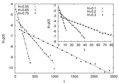
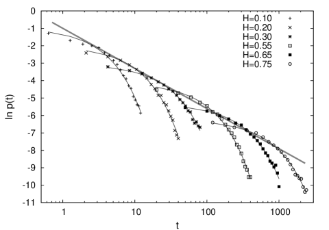
Figure 2: Top panel: Probability density function (PDF) of the escape time nicely demonstrating the exponential decay given by Eq. (2). The main plot depicts the persistent case ($H=0.55$, 0.65, 0.75), while in the inset we show the anti-persistent case ($H=0.1$, 0.2, and 0.3). Here we used the following simulations parameters: in the antipersistent case the time increment is $\delta t=0.001$, the number of samples $N_{\mathrm{stat}}=10^{5}$, the number of data points per sample $N_{\mathrm{max}}$ varied from $2^{13}\approx 8.2\times 10^{3}$ to $2^{21}\approx 2.1\times 10^{6}$, and finally the noise strength $D=0.25$; in the persistent case we used $\delta t=0.001$, $N_{\mathrm{stat}}=20000$, $N_{\mathrm{max}}=2^{20}\approx 10^{6}$, and $D=0.25$. Bottom panel: PDF of the escape time in a log-log representation. The decay curves have a common envelope $1/(et)$ depicted by the straight grey line, see text.

In our simulations we follow the motion of the test particle governed by the discrete Langevin equation (11) in the harmonic potential with one-sided truncation, Eq. (5). Once the particle crosses the point $x=\sqrt{2}$ it is removed, and the next particle started. This setup is depicted in Fig. 1.

We first focus on the probability density function (PDF) of the first escape time from the potential well. In Fig. 2 we demonstrate that, in analogy to the classical case ($H=1/2$) the probability density function (PDF) of the first escape time decays exponentially with time, see Eq. (2). This exponential decay is observed nicely in the simulations data over the entire range of the Hurst exponent. In the double-logarithmic plot in the bottom panel of Fig. 2 one can see a common envelope of the curves for all values of $H$. Indeed the shoulders of the individual exponential PDFs are located at points in time where $t=T$, i.e., where the value of the PDFs is exactly $1/(eT)$. This is the straight line plotted in Fig. 2, showing good agreement, with a slight underestimation for persistent Hurst exponents.

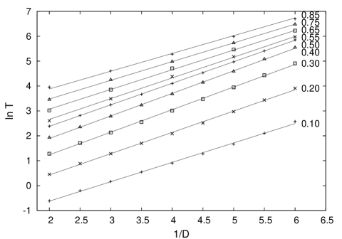
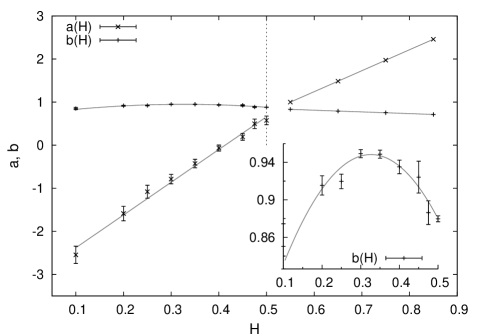
Figure 3: Top panel: Mean escape time $T$ as function of inverse noise intensity $1/D$ in logarithmic scale. The simulations results are shown for Hurst exponents $H=0.85$, 0.75, 0.65, 0.55, 0.5, 0.4, 0.3, 0.2, and 0.1 (top to bottom). The solid lines represent a linear fit. Bottom panel: Fitting coefficients $a(H)$ and $b(H)$ from Eq. (12). The inset shows $b(H)$ for the antipersistent case at higher resolution. The symbols represent the values of $a$ and $b$ from the simulations, while the solid lines show the respective fits with Eqs. (13) to (16). Simulations parameters: in the antipersistent case we used the time increment $\delta t=0.001$, number of samples $N_{\mathrm{stat}}=10^{5}$, and the data points per sample $N_{\mathrm{max}}$ varied from $2^{13}\approx 8.2\times 10^{3}$ to $2^{21}\approx 2.1\times 10^{6}$; in the persistent case $\delta t$ ranges from 0.01 to 0.001, $N_{\mathrm{stat}}=10^{6}$, and $N_{\mathrm{max}}$ varied from $2^{13}\approx 8.2\times 10^{3}$ to $2^{18}\approx 2.6\times 10^{5}$.

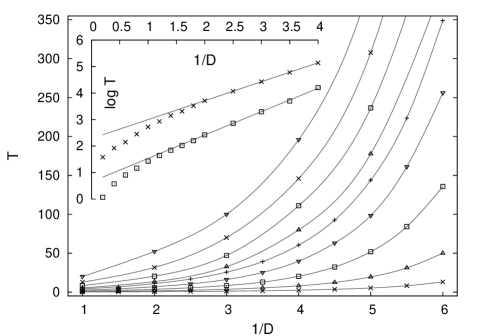
Figure 4: Mean escape time $T$ as function of inverse noise intensity $1/D$ in linear scale. Data points are the same as in Fig. 3. Again, the dots represent the simulations data, and the solid lines depict the exponential fit with the global fitting coefficients according to Eqs. (13) to (16). From top to bottom: Hurst exponent $H=0.85$ ($\triangledown$), $H=0.75$ ($\times$), $H=0.65$ ($\square$), $H=0.55$ ($\triangle$), $H=0.50$ ($+$), $H=0.40$ ($\triangledown$), $H=0.30$ (($\square$), $H=0.20$ ($\triangle$), $H=0.10$ ($\times$). Inset: Too high noise intensity violating the high barrier assumption leads to deviations from the exponential behavior. Hurst exponent $H=0.5$ ($\square$) and $H=0.8$ ($\times$).

In Fig. 3 we demonstrate that the mean escape time $T$ follows an exponential behavior as function of the inverse noise intensity, $1/D$, in analogy to the classical Kramers case. We observe that in both persistent and antipersistent cases this functional dependence may be approximated by a linear fit of the form

$$\ln T\left(D;H\right)=a(H)+\frac{b(H)}{D},$$ (12)

where both fitting coefficients $a$ and $b$ are functions of the Hurst exponent $H$. These, in turn, show different behavior for antipersitence and persistence of the motion:

(i) In the persistent case $1/2\leq H<1$ both coefficients are linear functions of the Hurst exponent. We found empirically from best fits that

$$a\left(H\geq 1/2\right) = a_{1}+a_{2}H,$$ (13)

$$b\left(H\geq 1/2\right) = b_{1}+b_{2}H,$$ (14)

where $a_{1}=-1.680$, $a_{2}=4.869$, $b_{1}=1.051$, and $b_{2}=-0.399$. The good quality of this linear description is seen in the bottom panel of Fig. 3.

(ii) Contrasting this behavior, in the antipersistent case the coefficient $a\left(H\right)$ is still well described by a linear $H$-dependence, while $b\left(H\right)$ is well represented by a parabolic dependence:

$$a\left(H\leq 1/2\right) = \tilde{a}_{1}+\tilde{a}_{2}H,$$ (15)

$$b\left(H\leq 1/2\right) = \tilde{b}_{1}+\tilde{b}_{2}H+\tilde{b}_{3}H^{2}.$$ (16)

The best fit parameters are determined as $\tilde{a}_{1}=-3.019$, $\tilde{a}_{2}=7.296$, $\tilde{b}_{1}=0.705$, $\tilde{b}_{2}=1.490$ and $\tilde{b}_{3}=-2.281$. Again, Fig. 3 demonstrates good agreement with this chosen $H$-dependence. In Fig. 4 we show the quality of these fits (solid curves) on a linear scale. Note the deviations from the exponential behavior when the noise intensity becomes too large [in our simulation for values $D>1$]. In that case the high barrier limit is violated and the results obtained herein are no more applicable, in correspondence to regular Brownian barrier crossing behavior.

The general agreement with the law (12) is excellent, keeping in mind that the error of the simulations data is of the magnitude of the points. Remarkably the characteristic escape time increases from low to high Hurst exponent. In other words, the less persistent motion shows the faster escape. This observation is consistent throughout our simulations. In particular this behavior is not qualitatively changed for a parabolic potential of the type (6) with symmetric cutoff.

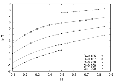
Figure 5: Mean escape time as a function of the Hurst exponent for different noise intensities $D$. The solid lines correspond to the fits used in Fig. 3, converted according to Eqs. (17) and (18).

In Fig. 5 the mean escape time is reanalyzed as a function of the Hurst exponent. In accordance with the results presented in Fig. 3, there is a parabolic dependence of $\ln T$ versus $H$ in the antipersistent case ($0<H<1/2$),

$$\ln T=\tilde{c}_{1}+\tilde{c}_{2}H+\tilde{c}_{3}H^{2},$$ (17)

where $\tilde{c}_{1}=\tilde{a}_{1}+\tilde{b}_{1}/D$, $\tilde{c}_{2}=\tilde{a}_{2}+\tilde{b}_{2}/D$, and $\tilde{c}_{3}=\tilde{b}_{3}/D$. In the persistent case $1/2<H<1$ the relation is linear, corresponding to

$$\ln T={c}_{1}+{c}_{2}H,$$ (18)

where $c_{1}=a_{1}+b_{1}/D$ and $c_{2}=a_{2}+b_{2}/D$. The agreement with the fit function is favorable, and the continuation between antipersistent and persistent cases appears relatively smooth. The latter supports the good convergence of the simulations algorithms used in the antipersistent and persistent regimes (see Appendix A). At the same time the difference between the behaviors in the two regimes (persistent versus antipersistent) is quite distinct.

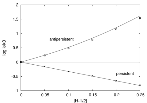
Figure 6: Relative escape rate $k\left(H\right)/k\left(H=1/2\right)$ as a function of $\left|H-1/2\right|$ for the persistent and antipersistent cases for $D=0.25$. The solid parabolic and straight lines are obtained from fits to the numerical data according to Eqs. (17) and (18), respectively. A fine coincidence is observed.

Fig. 6 shows an alternative way to represent the behavior from Figs. 3 and 5, namely, in terms of the ratio $k\left(H\right)/k\left(H=1/2\right)$ of the escape rates (that is, the inverse mean escape times) as function of the deviation $\left|H-1/2\right|$ from normal diffusion at $H=1/2$. The rates increase with decreasing Hurst exponent, i.e., the less persistent the motion is the higher becomes the corresponding rate. One can also see the difference between the parabolic dependence in the antipersistent case and the linear relation for persistent motion.

Finally in Fig. 7 we explore the distribution of the results for the mean escape time between different samples of only 60 trajectories. Again we see the increased escape time at higher Hurst exponent. We also clearly observe that the variation around the average values increases significantly for higher Hurst exponent. In particular the noise for the plotted case $H=0.3$ is consistently smaller than for the Brownian limit $H=1/2$.

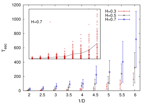
Figure 7: (Color online) Results for the mean escape time. Main graph: for three different values of the Hurst exponents ($H=0.3$, 0.5, and 0.7) we show the average value and the standard deviation around that value for different inverse noise intensities $1/D$. Note that $T_{esc}$ is evaluated at $1/D=2$, 2.5, $3,\ldots$. at each $H$ value. In the figure the results for different $H$ at each given value of $1/D$ are slightly shifted with respect to each other for illustrative purposes. Inset: values of the escape times for each individual out of 60 trajectories for $H=0.7$. The grey line connects the averages. In the simulations we used the time increment $\delta t=0.001$ and the number of points per trajectory $N_{\mathrm{max}}$ varied from $2^{11}\approx 2\times 10^{3}$ to $2^{20}\approx 10^{6}$.

III Analytical approach to FBM driven Kramers escape

In this Section we derive analytical results for the escape behavior driven by fractional Gaussian noise. In particular we concentrate on the mean escape time and the autocorrelation function for FBM in an harmonic potential. We compare the results to the numerical findings from the preceding Section.

III.1 Wilemski-Fixmann approximation

The investigation of first passage times for non-Markovian processes has a long history in mathematical literature, for instance, see Refs. Slepian ; Molchan ; Rice ; stratonovich , and appears in different fields of science, including chemical physics haenggi , polymer physics willemski ; szabo and neuroscience Igor-Tatiana . However, no general theory exists for such processes, and different approximations are used depending on whether the process is Gaussian or not, whether its trajectories are differentiable or not, etc. Our analytical approach to the escape problem considered herein is based on a special case of the Wilemski-Fixmann approximation (WFA)willemski used in polymer physics szabo . As shown in Ref. Igor_PRL the application of the WFA to a first passage problem corresponds to a renewal approximation redner ; hughes in which, however, the correct Green’s functions of the original non-renewal processes are used. The WFA is essentially a first approximation in the perturbative series derived by Likthman and Marques Marques , while higher approximations lead to quite involved expressions.

Our theoretical approach starts from the relation

$$G(x,t|x_{0},0) = \delta(x-x_{0})\delta(t)$$ (19)

$$+\int_{0}^{t}F(x,t^{\prime},x_{0},0)G(x,t|x,t^{\prime})dt^{\prime},$$

where $G(x,t|x_{0},0)$ is the conditional probability to find the particle at position $x$ at time $t$, provided that it started at $x_{0}$ at time $t=0$. Moreover $F(x,t,x_{0},0)$ represents the first passage time PDF to cross the distance $|x-x_{0}|$ during the time interval $t$, and $G\left(x,t|x,t^{\prime}\right)$ is the conditional probability to be at $x$ at time $t$, provided $x$ was visited earlier at time $t^{\prime}$. If the inequality $x_{0}\neq x$ holds the $\delta$-term can be omitted. For a continuous Markovian process Eq. (19) is exact. Its meaning is that a particle, having started at $x_{0}$ at time 0 and being at a site $x$ at time $t$, might have visited $x$ at some time $t^{\prime}$ before, departed from $x$, and returned redner ; hughes . For the non-Markovian case Eq. (19) neglects the correlations in the motion of the particle before and after the first passage through the point $x$. Such correlations lead to the dependence of the return probability (expressed through $G(x,t|x,t^{\prime})$) on the pre-history Igor_PRL , and can be taken into account systematically in higher order approximations involving multi-point distribution functions Marques . The approximation given by Eq. (19) may become incorrect in the case of strongly correlated (persistent) processes. In that case our numerical results still show exponential first passage time behavior corresponding to a finite mean first passage time, while the WFA breaks down, as will be shown below.

To proceed recall that according to Bayes’ formula, $G(x,t|x_{0},0)=P(x,t;x_{0},0)/P(x_{0},0)$ and $G(x,t|x,t^{\prime})=P(x,t;x,t^{\prime})/P(x,t^{\prime})$. Here $P(x,t;x,0)$ and $P(x,t)$ are the corresponding two- and one-point probability densities. Eq. (19) can therefore be rewritten in the form

$$P(x,t;x_{0},0) = P(x_{0},0)$$ (20)

$$\times\int_{0}^{t}F(x,t^{\prime},x_{0},0)\frac{P(x,t;x,t^{\prime})}{P(x,t^{\prime})}dt^{\prime}.$$

Integration with respect to $x_{0}$ in Eq. (20) leads to the expression

$$P(x,t)=\int_{0}^{t}F(x,t^{\prime})\frac{P(x,t;x,t^{\prime})}{P(x,t^{\prime})}dt^{\prime},$$ (21)

where

$$F(x,t^{\prime})=\int_{-\infty}^{\infty}P(x_{0},0)F(x,t^{\prime},x_{0},t)dx_{0}.$$ (22)

Thus, the first escape PDF $F$ is obtained as an average over the initial distribution.

In what follows we make use of the fact that in our numerical simulations the typical relaxation times for a particle in an harmonic potential well are much shorter than the typical mean escape times. Therefore the random process $x(t)$ can be considered as stationary, that is, $P(x,t)=P_{st}(x)$ and $P(x,t;x,t^{\prime})=P(x,x,t-t^{\prime})$. Transferring $P$ from the left hand side to the right of Eq. (21) we find

$$1=\int_{0}^{t}F(x,t^{\prime})\frac{P(x,x,t-t^{\prime})}{P_{st}^{2}(x)}dt^{\prime}.$$ (23)

This relation converts to an algebraic equation after Laplace transformation,

$$\frac{1}{s}=\tilde{F}(x,s)\frac{\tilde{P}(x,x,s)}{P_{st}^{2}(x)}.$$ (24)

Here we express the Laplace transform of a function $f(t)$ as $\tilde{f}(s)=\int_{0}^{\infty}f(t)\exp(-st)dt$. Since $P(x,x,t\to\infty)\to P_{st}^{2}(x)$, we see that $\tilde{P}(x,x,s\to 0)\to P_{st}^{2}(x)/s$, and for small $s$ we may expand $\tilde{P}(x,x,s)$ in the form

$$\tilde{P}(x,x,s)\approx\frac{P_{st}^{2}(x)}{s}+A(x)+O(s),$$ (25)

where we use the abbreviation

$$A(x) = \lim_{s\to 0}\left[\tilde{P}(x,x,s)-\frac{P_{st}^{2}(x)}{s}\right]$$ (26)

$$= \int_{0}^{\infty}\Big{[}P(x,x,t)-P_{st}^{2}(x)\Big{]}dt.$$

After inserting Eq. (25) into Eq. (24) we get

$$\tilde{F}(x,s)=\frac{P_{st}^{2}(x)}{s\tilde{P}(x,x,s)} \approx \frac{P_{st}^{2}(x)}{P_{st}^{2}(x)+A(x)s}$$ (27)

$$\approx 1-\frac{A(x)}{P_{st}^{2}(x)}s+\ldots.$$

Thus, with the use of Eq. (26), we find

$$T(x) = -\left.\frac{d}{ds}\tilde{F}(x,s)\right|_{s=0}$$ (28)

$$= \frac{A(x)}{P_{st}^{2}(x)}=\int_{0}^{\infty}\left[\frac{P(x,x,t)}{P_{st}^{2}(x)}-1\right]dt.$$

We will use this result below.

Before proceeding two remarks are in order: First, we note that in the theory developed here we use the ensemble average over initial values $x_{0}$, while in the simulations we use $x_{0}=0$ for all trajectories. Nevertheless, we can employ Eq. (27) since typically the relaxation time is much shorter than the mean escape time and, therefore, the system quickly converges to the stationary state, which is independent of the initial condition. And second, when writing Eq. (25) we implicitly assume that the mean escape time exists. This is in accordance with the numerical observation that the escape time PDF has the simple exponential form (2).

III.2 Mean escape time for Gaussian processes

To proceed we exploit the Gaussian property of FBM processes. We recall the expressions for one- and two-point Gaussian PDFs, namely,

$$P_{st}(x)=\frac{1}{\sqrt{2\pi\sigma^{2}}}\exp\left(-\frac{x^{2}}{2\sigma^{2}}\right),$$ (29)

where $\sigma^{2}=\left\langle x^{2}\right\rangle_{st}$ is the variance in the stationary state of a particle in an harmonic potential well. Moreover

$$P(x,y,t) = \frac{1}{2\pi\sigma_{x}\sigma_{y}\sqrt{1-g^{2}(t)}}$$ (30)

$$\times\exp\left\{-\frac{1}{2(1-g^{2})}\left(\frac{x^{2}}{\sigma_{x}^{2}}+\frac{y^{2}}{\sigma_{y}^{2}}-\frac{2gxy}{\sigma_{x}\sigma_{y}}\right)\right\},$$

where $g(t)$ is the normalized autocorrelation function in the stationary state,

$$g(x,y,\tau)=\frac{\left\langle x(t)y(t+\tau)\right\rangle_{st}}{\sigma_{x}\sigma_{y}}.$$ (31)

Thus, within our approximation

$$P(x,x,t)=\frac{1}{2\pi\sigma^{2}\sqrt{1-g^{2}}}\exp\left\{-\frac{x^{2}}{\sigma^{2}\left(1+g\right)}\right\},$$ (32)

and we obtain the mean time

$$T=\int_{0}^{\infty}\left\{\frac{1}{\sqrt{1-g^{2}(\tau)}}\exp\left[\frac{x^{2}}{\left\langle x^{2}\right\rangle_{st}}\frac{g(\tau)}{1+g(\tau)}\right]-1\right\}d\tau.$$ (33)

Here we identified

$$g(\tau)=\frac{\left\langle x(t)x(t+\tau)\right\rangle_{st}}{\left\langle x^{2}\right\rangle_{st}}.$$ (34)

Expressions $\langle x(t)x(t+\tau)\rangle_{st}$ and $\langle x^{2}\rangle_{st}$ are calculated in App. C.

III.3 Persistent and antipersistent cases

Consider now the asymptotic behavior of the integrand in expression (33) at $\tau\rightarrow\infty$,

$$\left\{...\right\} \mathop{\approx}\limits_{\tau\to\infty} \left[1+g^{2}(\tau)\right]\left[1+\frac{x_{esc}^{2}}{\left\langle x^{2}\right\rangle_{st}}\frac{g(\tau)}{1+g(\tau)}\right]-1$$ (35)

$$\approx \frac{x_{esc}^{2}}{\left\langle x^{2}\right\rangle_{st}}g(\tau).$$

Since $g(\tau)\sim\tau^{2H-2}$, the integrand decays slowly; the integral in Eq. (33) itself converges for $H<1/2$ and diverges for $H>1/2$.

Focusing at first on the antipersistent case we notice that according to Eq. (33) the main contribution comes from the integrand estimated at $g(\tau)\sim 1$, which immediately leads to

$$T\simeq\exp\left(\frac{1}{\left\langle x^{2}\right\rangle_{st}}\right),$$ (36)

being a kind of generalization of the standard transition-state arguments to the FBM case. Recalling that for our harmonic potential, $\left\langle x^{2}\right\rangle_{st}=D\Gamma(2H+1)$, we obtain an estimate for the coefficient $b(H)$ in the empirical formula for the escape time, Eq. (12). Namely, we find

$$b(H)=\frac{1}{\Gamma(2H+1)}.$$ (37)

Eq. (37) provides a surprisingly good approximation to the behavior of $b(H)$ obtained from the simulations, as shown in Fig. 8. In particular, approximation (37) shows the nontrivial maximum for intermediate $H$-values. Fig. 9 shows the values for the mean escape time obtained from our simulations of the antipersistent process with $0<H<1/2$, along with the behavior predicted by Eqs. (33) and (34).

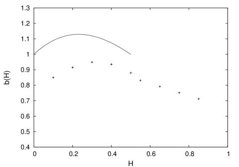
Figure 8: Coefficient $b(H)$ occurring in the empirical formula (12) for the mean escape time. Symbols: Values obtained from best fit. Solid line: Theoretical behavior described by Eq. (37).

In the persistent case the integral in expression (33) diverges. We show that a suitable truncation at some upper bound $\tau_{cut}$ leads to a quite good agreement with the behavior recovered from simulations. Physically such a truncation always exists due to the finiteness of the slow power-law decay of the autocorrelation function of fractional Gaussian noise. Thus, we would always expect finite mean escape times also in the persistent range. Because of the slow divergence of the integral for $T$, we may expect a weak dependence of the integral on the cutoff parameter $\tau_{cut}$ if only it is chosen large enough. Indeed, we found in our numerical simulations that the value $\tau_{cut}=18$ already gives good agreement with the numerical simulation, see Fig. 9 bottom.

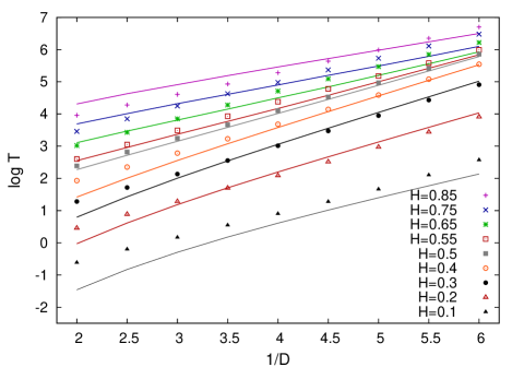
Figure 9: (Color online.) Mean escape time $T$ as function of inverse noise intensity, $1/D$. Symbols: simulations results. The solid lines show the analytical result given by Eqs. (33) and (34) in the antipersistent case $0<H<1/2$. For persistent motion $1/2<H<1$ the solid lines represent a fit by Eqs. (33) and (34) based on numerical truncation of the integral in Eq. (33) with cutoff time $\tau_{cut}=18$.

IV Summary

In this work we present an extensive analysis of the generalized Kramers escape from a potential well for a particle subject to fractional Brownian motion. Specifically we considered a particle whose motion is governed by the Langevin equation driven by external fractional Gaussian noise. The motion we consider is thus not subject to the fluctuation dissipation theorem. Potential applications for such behavior may, for instance, include geo- and astrophysical fluctuations, stock market pricing, or teletraffic.

Based on simulations and analytical derivations we showed that, despite the driving fractional Gaussian noise, the escape dynamics preserved the classical exponential shape of the distribution of escape times. Deviations from the behavior for regular Gaussian white noise are found in the activation dependence of the mean escape time on the noise intensity at different values of the Hurst exponent $H$.

The escape turns out to slow down for increasing value of the Hurst exponent. Thus in the persistent case $1/2<H<1$ the escape is slower than in the antipersistent case $0<H<1/2$, and the latter is faster than for ordinary Brownian case. This somewhat surprising result is in accordance with previous results for the first passage time Molchan , where the scaling exponent of the first passage time distribution decreases for increasing $H$. We note that this observation is not restricted to the asymmetrically truncated harmonic potential used in this work, but also occurs for a symmetric truncation of the harmonic potential at $x=\pm\sqrt{2}$.

Analyzing the detailed behavior of the mean escape time we find that the logarithm, $\log T$ in the entire simulations range $H=0.1,\ldots,0.85$ depends linearly on the inverse noise intensity, $1/D$. This activation dependence is thus preserved for both antipersistent and persistent cases. Conversely, the behavior of $\log T$ on the Hurst exponent shows a linear dependence in the persistent case, while in the antipersistent case we find a nonlinear dependence.

We note that fractional Brownian motion is an ergodic process in the sense that time and ensemble averages coincide, albeit the convergence to ergodicity is algebraically slow with the measurement time deng . For sufficiently long averaging times the dynamic behavior of time and ensemble averages of individual trajectories should therefore be identical. This contrasts the behavior for continuous time random walk processes with diverging characteristic waiting times web or with correlations in waiting times or jump lengths vincent1 .

The understanding of fractional Brownian motion in several aspects remains formidable. We expect that this work contributes toward the demystification of this seemingly simple stochastic process.

Appendix A Description of FBM generators

Here we briefly describe the generators with which we simulated FBM. It should be noted that the generators provide best results for either the antipersistent case $0<H<1/2$ or for the persistent case $1/2<H<1$.

A fast and precise (see the tests in Appendix B) generator for fractional Gaussian noise in the anti-persistent case is described in Ref. fGnAlg1 . In brief, the idea is as follows.

First, we define a function

$$R_{x}(n)=\left\{\begin{array}[]{ll}2^{-1}\left[1-(n/N_{\mathrm{max}})^{2H}\right],&0\leq n\leq N_{\mathrm{max}}\\[5.69046pt] R_{x}(2N_{\mathrm{max}}-n),&N_{\mathrm{max}}<n<2N_{\mathrm{max}}\end{array}\right.$$ (38)

where $H$ is the Hurst parameter ($0<H<1/2$), $n$ is the number of steps corresponding to time in the continuous time limit, and $N_{\mathrm{max}}$ is the length of the random sample. Second, we perform a discrete Fourier transformation of Eq. (38), with $S_{x}(k)=F\{R_{x}(n)\}.$

We then define

$$X(k)=\left\{\begin{array}[]{ll}0,&k=0\\[5.69046pt] \exp(i\theta_{k})\xi(k)\sqrt{S_{x}(k)},&0<k<N_{\mathrm{max}}\\[5.69046pt] \xi(k)\sqrt{S_{x}(k)},&k=N_{\mathrm{max}}\\[5.69046pt] X^{*}(2N_{\mathrm{max}}-k),&N_{\mathrm{max}}<k<2N_{\mathrm{max}},\end{array}\right.$$ (39)

where the symbol $*$ stands for complex conjugation, $\theta_{k}$ are uniform random numbers from $[0,2\pi)$, and $\xi(k)$ are Gaussian random variables with zero mean and variance equal to 2. All random variables are independent of each other.

Finally, we set $y(n)=x(n)-x(0),$ where $x(n)=F^{-1}\left\{X(k)\right\}$ is the inverse Fourier transformation of Eq. (39). The quantity $y(n)$ represents a free [i.e., in absence of an external force] fractional Brownian trajectory which is to be differentiated with respect to time, to obtain fractional Gaussian random numbers. Since the variance $\left\langle\xi^{2}\right\rangle$ depends on the number of steps $N_{\mathrm{max}}$, it is normalized such that $\left\langle\xi^{2}\right\rangle=2$.

Despite the availability of several exact simulation methods, for the persistent case we chose an approximate but efficient simulation method. This generator exploits the spectral properties of fractional Gaussian noise fGnAlg2 . The method uses the following steps:

(i) Take white Gaussian noise $\xi(t)$, where $t$ is an integer.

(ii) Calculate the spectral density of this Gaussian noise and perform a Fourier transformation, $S(k)=F\{\xi(t)\}$.

(iii) Introduce correlations multiplying it by $1/k^{H-1/2}$, where $1/2<H<1$.

(iv) Inverse Fourier transform $\xi_{H}(t)=F^{-1}\{S(k)k^{1/2-H}\}$, to obtain approximate fractional Gaussian noise with the index $H$.

(v) Normalize the noise.

In Appendix B we demonstrate that this method reliably produces FBM.

We note that since we approximate the integral representation, this creates two types of errors, a ‘low frequency’ one due to the truncation of the limit of integration and a ‘high frequency’ one caused by replacing the integral by a sum. By using various tests, we estimated the best discretization parameters. We used the maximum sample length of $2^{24}\approx 1.7\times 10^{7}$ steps, the time increment varying within the interval $[0.001,0.01]$.

Appendix B Testing the numerical algorithm

To check our simulations algorithm based on numerical integration of the Langevin equation (11) we performed a number of tests to validate the FBM we create with the generators sketched in Appendix A.

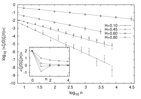
Figure 10: Absolute value of the autocorrelation function of fractional Gaussian noise for the entire range of the Hurst exponent $H$ in a log-log scale as function of the number of time steps $n$. Inset: autocorrelation functions with the same Hurst indices for small numbers of steps $n$ on a linear scale. The numerical results are shown for $H=0.10$, 0.45, 0.60, and 0.80. The solid lines in the main graph correspond to the analytical solution (8). Simulations parameters: number of simulated samples $N_{\mathrm{stat}}=20,000$, each of length $N_{\mathrm{max}}=2^{13}\approx 8.2\times 10^{3}$ for the antipersistent case, and $2^{15}\approx 3.3\times 10^{4}$ for the persistent case, respectively.

First, we calculated the autocorrelation function of the fractional Gaussian noise. As shown in Fig. 10, the simulated data show excellent agreement with the analyical result (solid lines) given by Eq. (8) for discrete time steps.

Second, we calculated the position mean squared displacement

$$\langle x_{H}(t)^{2}\rangle=2Dt^{2H}.$$ (40)

and two-point correlation function

$$\langle x_{H}(t_{1})x_{H}(t_{2})\rangle=D(t_{1}^{2H}+t_{2}^{2H}-|t_{1}-t_{2}|^{2H}).$$ (41)

of free FBM, and compare with the analytical expressions for FBM in discrete time $n$ with time increments $\delta t=1$,

$$\langle x_{H}(n)^{2}\rangle = 2Dn^{2H},$$ (42)

$$\langle x_{H}(n)x_{H}(1)\rangle = D\left(1+n^{2H}-|n-1|^{2H}\right).$$ (43)

As demonstrated in Figs. 11 and 12, respectively, the agreement is excellent.

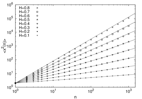
Figure 11: Mean squared displacement for free FBM in log-log representation. The solid lines show the analytical expression (42) while the symbols depict the simulations for different Hurst parameters ranging from $H=0.1$ (lowest curve) to $H=0.8$ (uppermost curve). Here, $D$ was taken to be equal to $1$, the time step $\delta t=1$, $N_{\mathrm{stat}}=20,000$, and $N_{\mathrm{max}}=2^{10}\approx 10^{3}$.

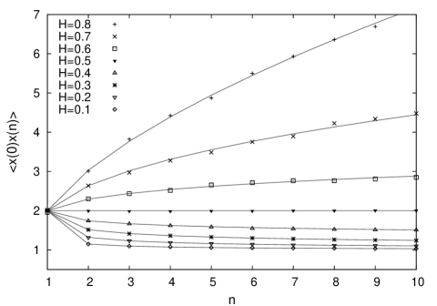
Figure 12: Position autocorelation function of free fBm. The solid lines show the analytical expression (43) while the symbols depict the simulations for different Hurst parameters ranging from $H=0.1$ (lowest curve) to $H=0.8$ (uppermost curve). Again, $D$ was taken to be equal to $1$, the time increment $\delta t=1$, $N_{\mathrm{stat}}=2\times 10^{6}$, and $N_{\mathrm{max}}=64$.

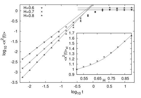
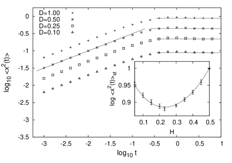
Figure 13: Mean squared displacement of FBM in an harmonic potential. Top panel: mean squared displacement for fixed $D=1.0$ and varying Hurst index. Bottom panel: mean squared displacement for fixed Hurst index $H=0.25$ and four different values of the noise intensity. The solid lines show the asymptotes of free FBM ($t^{2H}$ power-laws corresponding to straight lines in the log-log scale) and stationary states (horizontal lines). Insets: stationary values of the mean squared displacements as functions of $H$ for fixed $D=1.0$. The points in all graphs represent the simulations results for the following parameters: time increment $\delta t=0.01$, number of samples $N_{\mathrm{stat}}=10^{6}$, and number of steps per sample $N_{\mathrm{max}}=2^{10}\approx 10^{3}$ for both persistent and antipersistent cases.

Third, solving Eq. (11) we calculated the mean squared displacement for a particle in an infinite harmonic potential well, as shown in Fig. 13. The initial condition was $x=0$, at the bottom of the potential well. The asymptotic analytical behaviors are represented by the initial free behavior $\langle x^{2}(t)\rangle\simeq t^{2H}$ and the terminal saturation value $\left\langle x^{2}(t)\right\rangle_{\mathrm{st}}=D\Gamma(1+2H)$ at $t\rightarrow\infty$ (for details, see Appendix C). This demonstrates that our generators also produce reliable behavior in an external potential.

Finally, we performed a simulation of a free particle escaping from a semi-infinite axis with absorbing boundary under the influence of fractional Gaussian noise, see Fig. 14. The observed scaling of the first passage time PDF $p\left(t\right)$ compares very favourably with the analytical result from Refs. Molchan :

$$p(t)\simeq t^{-2+H}.$$ (44)

Note that this relation cannot be obtained by the method of images, despite the fact that FBM is a Gaussian process. Also note that the slope of this power-law becomes flatter for increasing Hurst coefficient: the escape is slower for a more persistent FBM, i.e., a motion whose mean squared displacement grows faster. This a priori surprising behavior is also seen for the escape from the potential well studied herein.

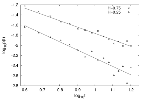
Figure 14: First passage time PDF of FBM on a semi-infinite axis with absorbing boundary condition. The solid lines demonstrate the respective analytical slopes. Parameters in the antipersistent case: $H=0.25$, time increment $\delta t=0.001$, number of samples $N_{\mathrm{stat}}=100,000$ and number of steps per sample $N_{\mathrm{max}}=2^{17}\approx 1.3\times 10^{5}$. In the persistent case we used $H=0.75$, $\delta t=0.001$, $N_{\mathrm{stat}}=20,000$, and $N_{\mathrm{max}}=2^{13}\approx 8.2\times 10^{3}$.

Appendix C Variance and autocorrelation function for FBM in a harmonic potential well.

We now consider FBM in a harmonic potential, as described by the Langevin equation (compare with Eq. (10))

$$\frac{dx(t)}{dt}=-ax+D^{1/2}\xi_{H}(t),$$ (45)

where we introduce the prefactor $a$ which allows us to consider the harmonic potential ($a=1$) and a free FBM ($a=0$) as well. The solution of Eq. (45) with the initial condition $x(t=0)=0$ is

$$x(t)=D^{1/2}\int_{0}^{t}e^{-a(t-t^{\prime})}\xi_{H}(t^{\prime})dt^{\prime}.$$ (46)

Then, the ACF function

$$\left\langle x(t_{1})x(t_{2})\right\rangle=De^{-2at}\int\limits_{0}^{t_{1}}{dt^{\prime}\int\limits_{0}^{t_{2}}{dt^{\prime\prime}e^{a(t^{\prime}+t^{\prime\prime})}\left\langle\xi(t^{\prime})\xi(t^{\prime\prime})\right\rangle}}$$

$$=-De^{-2at}\int\limits_{0}^{t_{1}}{dt^{\prime}\int\limits_{0}^{t_{2}}{dt^{\prime\prime}e^{a(t^{\prime}+t^{\prime\prime})}\frac{{\partial^{2}}}{{\partial t^{\prime}\partial t^{\prime\prime}}}\left|{t^{\prime}-t^{\prime\prime}}\right|^{2H}}}.$$ (47)

Now, if $t_{2}-t_{1}=\tau$, $\tau>0$, after some lengthy calculations we get Eq. (C):

$$\left\langle x(t)x(t+\tau)\right\rangle = D\Bigg{\{}e^{-a(t+\tau)}t^{2H}+e^{-at}(t+\tau)^{2H}-\tau^{2H}$$

$$- \frac{2a^{2}-1}{2a(2H+1)}\Big{[}t^{2H+1}e^{-a(2t+\tau)}M(2H+1;2H+2;at)$$

$$+ (t+\tau)^{2H+1}e^{-a(2t+\tau)}M(2H+1;2H+2;a(t+\tau))$$

$$- \ \tau^{2H+1}e^{-a\tau}M(2H+1;2H+2;a\tau)\Big{]}$$

$$- \frac{1}{2}a^{-2(H+1)}\left(2a^{2}-1\right)\Big{[}e^{a\tau}(\Gamma(2H+1;a(t+\tau))-\Gamma(2H+1;a\tau))$$

$$+ e^{-a\tau}(\Gamma(2H+1;at)-\Gamma(2H+1))\Big{]}\Bigg{\}}.$$

Assuming $a=1$,

$$\left\langle x(t)x(t+\tau)\right\rangle = D\Bigg{\{}e^{-(t+\tau)}t^{2H}-\tau^{2H}+e^{-t}(t+\tau)^{2H}$$

$$+ \frac{1}{2}e^{-\tau}\left[\Gamma(2H+1)-\Gamma(2H+1;t)+\frac{\tau^{2H+1}}{2H+1}M(2H+1;2H+2;\tau)\right]$$

$$- \frac{1}{2}e^{-2t-\tau}\left[\frac{t^{2H+1}}{2H+1}M(2H+1;2H+2;t)+\frac{(t+\tau)^{2H+1}}{2H+1}M(2H+1;2H+2;t+\tau)\right]$$

$$+ \frac{1}{2}e^{\tau}\left[\Gamma(2H+1;\tau)-\Gamma(2H+1;t+\tau)\right]\Bigg{\}}.$$

Here, $\Gamma(a,b)$ is the incomplete $\Gamma$-function, and $M$ denotes the Kummer function Abramowitz . In the stationary state ($t\to\infty$) the autocorrelation function Eq. (C) yields

$$\left\langle x(t)x(t+\tau)\right\rangle_{st}=D\Bigg{\{}\left[e^{-\tau}\Gamma(2H+1)+e^{\tau}\Gamma(2H+1,\tau)\right]$$

$$+\frac{\tau^{2H+1}e^{-\tau}}{2(2H+1)}M(2H+1;2H+2,\tau)-\tau^{2H}\Bigg{\}}.$$ (50)

In order to obtain the variance we take $\tau=0$ in Eq. (C):

$$\left\langle{x^{2}\left(t\right)}\right\rangle = D\Bigg{\{}2t^{2H}e^{-t}+\left[\Gamma\left(1+2H\right)-\Gamma\left(1+2H,t\right)\right]$$

$$- \frac{t^{2H+1}}{2H+1}e^{-2t}M(2H+1;2H+2;t)\Bigg{\}}.$$

Now, the stationary variance is:

$$\left\langle x^{2}\right\rangle_{st}=D\Gamma(2H+1).$$ (51)

Note that at $\tau=0$ Eq. (50) reduces to Eq. (51), whereas for $H=1/2$ it gives $\left\langle x(t)x(t+\tau)\right\rangle_{st}=De^{-\tau}$, the autocorrelation function of the Ornstein-Uhlenbeck process. Taking the asymptotics of the incomplete $\Gamma$-function and the Kummer function, one may easily see that $\left\langle x(t)x(t+\tau)\right\rangle_{st}\approx 2DH(2H-1)\tau^{2H-2}$ at $\tau\to\infty$.

The autocorrelation function of free fBm can be naturally obtained by placing $a=0$ in Eq. (C):

$$\left\langle x(t)x(t+\tau)\right\rangle=D\left\{t^{2h}+(t+\tau)^{2h}-\tau^{2h}\right\},$$ (52)

that matches the well-known relation Qian .

Appendix D Mean escape time and first escape time PDF for harmonic potential truncated from both sides

In this Appendix we consider the Kramers problem for an harmonic potential, but this time we introduce a cutoff on both sides, that is, at $x=\pm\sqrt{2}$, and evaluate the same dependencies (see Figures 15 and 16).

One can observe that qualitatively there is no difference in behaviour with the case of the one-side truncated potential. Indeed, the escape is faster when lowering the Hurst parameter; the escape time PDF remains exponential and so does the mean escape time. Again, the MET may be fitted with the following function:

$$T(H\leq 0.5) = \exp(ax^{2}+bx+c)$$

$$T(H>0.5) = \exp(b^{\prime}x+c^{\prime}),$$ (53)

where $a,b,c,b^{\prime},c^{\prime}$ are some constants depending on $D$.

Figure 15: First escape time PDF for harmonic potential truncated from both sides. Points are the simulation data, solid lines stand for linear fitting. Simulation details are the following: for the antipersistent case $D=0.25$, $\delta t=0.001$, $N_{\mathrm{max}}=131072$, $N_{\mathrm{stat}}=10^{5}$; for the persistent case $D=0.25,\delta t=0.002,N_{\mathrm{max}}=131072,N_{\mathrm{stat}}=10^{5}$.

Figure 16: Mean escape time as function of the Hurst parameter for harmonic potential truncated from both sides. Points are the simulation data, solid lines stand for fitting with Eq. (D). Simulation details are the following: for both antipersistent and persistent cases $\delta t$ varied from $0.001$ to $0.005$, $N_{\mathrm{stat}}=10^{5}$, $N_{\mathrm{max}}=2^{13}\ldots 2^{21}\approx 8\times 10^{3}\ldots 2\times 10^{6}$.

References

- (1) Y. Sinai, Theor. Prob. Appl. 27, 256 (1982).
- (2) J. Dräger and J. Klafter, Phys. Rev. Lett. 84, 5998 (2000).
- (3) V. Tejedor and R. Metzler, J. Phys. A 43, 082002 (2010).
- (4) L. F. Richardson, Proc. Roy. Soc. London A 110, 709 (1926).
- (5) G. Boffetta and I. M. Sokolov, Phys. Rev. Lett. 88, 094501 (2002).
- (6) J.-P. Bouchaud and A. Georges, Phys. Rep. 195, 127 (1990).
- (7) R. Metzler and J. Klafter, Phys. Rep. 339, 1 (2000); J. Phys. A 37, R161 (2004).
- (8) H. Scher and E. W. Montroll, Phys. Rev. B 12, 2455 (1975);
- (9) G. Pfister and H. Scher, Adv. Phys. 27, 747 (1978); Q. Gu, E. A. Schiff, S. Grebner, and R. Schwartz, Phys. Rev. Lett. 76, 3196 (1996).
- (10) H. Scher, G. Margolin, R. Metzler, J. Klafter, and B. Berkowitz, Geophys. Res. Lett. 29, 1061 (2002); B. Berkowitz, A. Cortis, M. Dentz and H. Scher, Reviews of Geophysics, 44, RG2003 (2006).
- (11) A. Klemm, R. Metzler, and R. Kimmich, Phys. Rev. E 65, 021112 (2002); S. Havlin and D. ben-Avraham, Adv. Phys. 36, 695 (1987).
- (12) A. Caspi, R. Granek, and M. Elbaum, Phys. Rev. Lett. 85, 5655 (2000); I. M. Tolić-Nørrelykke et al., ibid. 93, 078102 (2004); I. Golding and E. C. Cox, ibid. 96, 098102 (2006); H. Yang et al., Science 302, 262 (2003); M. Weiss, M. Elsner, F. Kartberg, and T. Nilsson, Biophys. J. 87, 3518 (2004); G. Seisenberger et al., Science 294, 1929 (2001).
- (13) I. Y. Wong et al., Phys. Rev. Lett. 92, 178101(2004); W. Pan et al., ibid. 102, 058101 (2009); D. Banks and C. Fradin, ibid. 89, 2960 (2005).
- (14) A. Caspi, R. Granek, and M. Elbaum, Phys. Rev. E 66, 011916 (2002).
- (15) G. Matheron and G. de Marsily, Water Res. Res. 16, 901 (1980).
- (16) T. H. Solomon, E. R. Weeks, and H. L. Swinney, Phys. Rev. Lett. 71, 3975 (1993).
- (17) S. Stapf, R. Kimmich, and R.-O. Seitter, Phys. Rev. Lett. 75, 2855 (1995); O. V. Bychuk and B. O’Shaugnessy, J. Chem. Phys. 101, 772 (1994); A. V. Chechkin, I. M. Zaid, M. A. Lomholt, I. M. Sokolov, and R. Metzler, Phys. Rev. E 79, 040105(R) (2009).
- (18) J. Klafter, A. Blumen and M. F. Shlesinger, Phys. Rev. A 35, 3081 (1987).
- (19) R. Metzler and J. Klafter, Chem. Phys. Lett. 321, 238 (2000).
- (20) P. D. Ditlevsen, Phys. Rev. E 60, 172 (1999).
- (21) A. V. Chechkin, V. Yu. Gonchar, J. Klafter, and R. Metzler, Europhys. Lett. 72, 348 (2005); A. V. Chechkin, O. Yu. Sliusarenko, J. Klafter, and R. Metzler, Phys. Rev. E. 75, 041101 (2007).
- (22) P. Imkeller and I. Pavlyukevich, J. Phys. A 39, L237 (2006).
- (23) A. N. Kolmogorov, Dokl. Acad. Sci. USSR 26, 115 (1940).
- (24) B. B. Mandelbrot and J. W. van Ness, SIAM Rev. 1, 422 (1968). Compare also B. B. Mandelbrot, Physica Scripta 32, 257 (1985).
- (25) A. Yaglom, Correlation theory of stationary and related random functions (Springer, Berlin, 1987).
- (26) H. Qian, Fractional Brownian Motion and Fractional Gaussian Noise. In G. Rangarajan and M.Z. Ding (eds), Processes with Long-Range Correlations (Springer, Lecture Notes in Physics, Vol.621), pp.22-33.
- (27) D. Panja, E-print arXiv:0912.2331.
- (28) L. Lizana and T. Ambjörnsson, Phys. Rev. Lett. 100, 200601 (2008); Phys. Rev. E 80, 051103 (2009).
- (29) G. Guigas and M. Weiss, Biophys. J. 94, 90 (2008); J. Szymanski and M. Weiss, Phys. Rev. Lett. 103, 038102 (2009); V. Tejedor et al, Biophys J. (at press).
- (30) H. E. Hurst, Trans. Amer. Soc. Civil Eng. 116, 400 (1951).
- (31) T. N. Palmer, G. J. Shutts, R. Hagedorn, F. J. Doblas-Reyes, T. Jung, and M. Leutbecher, Ann. Rev. Earth Planet. Sci. 33, 163 (2005).
- (32) I. Simonsen, Physica A 322, 597 (2003); N. E. Frangos, S. D. Vrontos, and A. N. Yannacopoulos, Appl. Stochast. Models in Business and Industry 23, 403 (2007).
- (33) T. Mikosch, S. Rednick, H. Rootzén, and A. Stegemann, Ann. Appl. Prob. 12, 23 (2002).
- (34) M. Ding and W. Yang, Phys. Rev. E 52, 207 (1995); J. Krug et al. Phys. Rev. E 56, 2702 (1997); G.M. Molchan. Commun. Math. Phys. 205 97 (1999).
- (35) S. Burov and E. Barkai, Phys. Rev. Lett. 100, 070601 (2008).
- (36) E. Barkai and R. Silbey, Phys. Rev. Lett. 102, 050602 (2009).
- (37) A. Romero, J. M. Sancho, and K. Lindenberg, Fluct. and Noise Lett. 2, L79 (2002).
- (38) I. Goychuk and P. Hänggi, Phys. Rev. Lett. 99, 200601 (2007); compare also I. Goychuk E-print arXiv:0905.082.
- (39) Yu. L. Klimontovich, Turbulent motion and the structure of chaos: a new approach to the statistical theory of open systems (Kluwer, Dordrecht, The Netherlands, 1992).
- (40) H. A. Kramers, Physica A 7, 284 (1940).
- (41) S. Chandrasekhar, Rev. Mod. Phys. 15 1 (1943).
- (42) H. Risken, The Fokker-Planck equation (Springer-Verlag, Berlin, 1989).
- (43) B.S. Lowen Methodology and Computing in Applied Probability 1:4, 445 (1999).
- (44) A.V. Chechkin and V.Yu. Gonchar, Chaos, Solitons and Fractals 12, 391 (2000).
- (45) D. Slepian, Bell Syst. Tech. J. 41, 463 (1962).
- (46) S. O. Rice, Bell Syst. Tech. J. 23, 282 (1944); ibid. 24, 46 (1945), reproduced in Noise and Stochastic Processes, edited by N. Wax (Dover, New York, NY, 1954).
- (47) R. L. Stratonovich, Topics in the theory if random noise, Vol. II (Gordon and Breach, New York, NY, 1967).
- (48) P. Hänggi and P. Jung, Adv. Chem. Phys. 89, 239 (1995).
- (49) G. Wilemski and M. Fixman, J. Chem. Phys. 60, 866 (1974); ibid., 878 (1974).
- (50) A. Szabo, K. Schulten, Z. Schulten, J. Chem. Phys. 72, 4350 (1980).
- (51) T. Verechtchaguina, I.M. Sokolov, and L. Schimansky-Geier, Phys. Rev. E 73, 031108 (2006).
- (52) I. M. Sokolov, Phys. Rev. Lett. 90, 080601 (2003).
- (53) S. Redner, A guide to first passage processes (Cambridge University Press, Cambridge, UK, 2001).
- (54) B. D. Hughes, Random walks and random environments. Vol. 1: Random Walks (Clarendon Press, Oxford, UK, 1995). Cf. chapter 3.2.
- (55) A.E. Likthman, C.M. Marques, Europhys. Lett. 75, 971 (2006).
- (56) W. H. Deng and E. Barkai, Phys. Rev. E 79, 011112 (2009); J.-H. Jeon and R. Metzler, Phys. Rev. E (at press).
- (57) A. Lubelski, I. M. Sokolov, and J. Klafter, Phys. Rev. Lett. 100, 250602 (2008); Y. He, S. Burov, R. Metzler, and E. Barkai, ibid. 101, 058101 (2008); R. Metzler, V. Tejedor, J.-H. Jeon, Y. He, W. Deng, S. Burov, and E. Barkai, Acta Phys. Polonica B 40, 1315 (2009); T. Neusius, I. M. Sokolov, and J. C. Smith, Phys. Rev. E 80, 011109 (2009); S. Burov, R. Metzler, and E. Barkai (unpublished).
- (58) M. Abramowitz, I.A. Stegun, Handbook of Mathematical Functions (National Bureau of Standards, Tenth Printing, USA, 1972).