Galactic electrons and positrons at the Earth:
new estimate of the primary and secondary fluxes
Abstract
Context. The so-called excess of cosmic ray (CR) positrons observed by the PAMELA satellite up to 100 GeV has led to many interpretation attempts, from standard astrophysics to a possible exotic contribution from dark matter annihilation or decay. The Fermi data subsequently obtained about CR electrons and positrons in the range 0.02-1 TeV, and HESS data above 1 TeV have provided additional information about the leptonic content of local Galactic CRs.
Aims. We analyse predictions of the CR lepton fluxes at the Earth of both secondary and primary origins, evaluate the theoretical uncertainties, and determine their level of consistency with respect to the available data.
Methods. For propagation, we use a relativistic treatment of the energy losses for which we provide useful parameterizations. We compute the secondary components by improving on the method that we derived earlier for positrons. For primaries, we estimate the contributions from astrophysical sources (supernova remnants and pulsars) by considering all known local objects within 2 kpc and a smooth distribution beyond.
Results. We find that the electron flux in the energy range 5-30 GeV is well reproduced by a smooth distant distribution of sources with index , while local sources dominate the flux at higher energy. For positrons, local pulsars have an important effect above 5-10 GeV. Uncertainties affecting the source modeling and propagation are degenerate and each translates into about one order of magnitude error in terms of local flux. The spectral shape at high energy is weakly correlated with the spectral indices of local sources, but more strongly with the hierarchy in their distance, age and power. Despite the large theoretical errors that we describe, our global and self-consistent analysis can explain all available data without over-tuning the parameters, and therefore without the need to consider any exotic physics.
Conclusions. Though a standard paradigm of Galactic CRs is well established, our results show that we can hardly talk about any standard model of CR leptons, because of the very large theoretical uncertainties. Our analysis provides details about the impact of these uncertainties, thereby sketching a roadmap for future improvements.
Key Words.:
(ISM:) cosmic raysdelahaye@lapp.in2p3.fr
lavalle@to.infn.it
lineros@to.infn.it
Preprint DFTT-51/2009 and LAPTH-1339/09
1 Introduction
Cosmic ray (CR) electrons and positrons111Hereafter, electrons will denote both electrons and positrons, unless specified. constitute % of the CR budget at the Earth in the GeV-TeV energy range, and provide interesting means of probing the acceleration processes in CR sources, propagation phenomenology, and the interstellar environment itself, complementary to protons (e.g., Blandford & Eichler 1987). At energies 100 GeV, their observed properties are mostly set by the very local environment. Their typical propagation scale is indeed limited to the kpc scale because of the very efficient electromagnetic energy losses caused by Compton scattering with the interstellar radiation fields (ISRF), the cosmic microwave background (CMB), and the magnetic field (Jones 1965; Blumenthal & Gould 1970). High energy CR electrons are produced directly by well-known astrophysical CR accelerators such as supernova remnants (SNRs) and pulsars, in which case they are referred to as primary electrons. They can also be created by secondary processes, mostly nuclear interactions of cosmic protons and light nuclei with the interstellar medium (ISM) gas concentrated in the Galactic disk (spallation), in which case they are referred to as secondary electrons. Because they have been assumed to hardly be produced in astrophysical sources, positrons have been proposed as potential tracers of new physics, in particular the annihilation or decay of dark matter (Silk & Srednicki 1984). Although the main theoretical ideas regarding the origin and propagation of cosmic electrons were formalized a long time ago in the seminal monograph of Ginzburg & Syrovatskii (1964), their ongoing measurements are still far from being completely understood.
The observation by the PAMELA satellite (PAMELA Collaboration et al. 2009) of a rising positron fraction up to 100 GeV has triggered a considerable amount of interpretation attempts. Estimates of the cosmic electron and positron fluxes were first calculated in detail in Moskalenko & Strong (1998), where only secondaries were considered for positrons, that fail to match the PAMELA data. We derived novel predictions of the secondary positron flux at the Earth, with a particular focus on sizing the theoretical errors caused by uncertainties in spallation cross-sections, in the modeling of the progenitor interstellar (IS) CR flux, in the characterization of the energy losses, and in the propagation parameters (Delahaye et al. 2009). Although the overall theoretical uncertainty is about one order of magnitude, we have still shown that a rising positron fraction was not expected unless a very soft electron spectrum was considered. Even in that case, however, we have also illustrated how difficult it was to accommodate a good fit to the PAMELA data in spectral shape as well as in amplitude. This soft electron spectrum is at the lowest statistical edge of the current electron cosmic ray data below 30 GeV. Likewise, it is not supported by the unprecedented measurements performed with the Fermi satellite between 20 GeV and 1 TeV of CR electrons plus positrons (Abdo et al. 2009b), which sets the true denominator of the positron fraction. At this stage, separate data of positrons and electrons would be of particular interest and would provide stronger grounds to any interpretation attempt, but, unfortunately, are not yet available. Nevertheless, from both predictions of the secondary positron flux and the current data, it appears unlikely that this increase observed in the positron fraction is purely of secondary origin. Therefore, this positron excess points towards the existence of primary sources of positrons in the neighborhood. Note finally that the cut-off in the electron flux observed by HESS around 3 TeV provides interesting and complementary information (Aharonian et al. 2008).
It has long been demonstrated that astrophysical sources may supply this extra-yield of cosmic positrons. For instance, as discussed by Boulares (1989) (see also e.g. Aharonian et al. 1995; Chi et al. 1996; Zhang & Cheng 2001), pulsars could provide sizable contributions to the positron flux from pair conversions of -rays in the strong magnetic fields that they host. This has been recently revisited by several authors (e.g. Hooper et al. 2009; Yüksel et al. 2009; Profumo 2008; Malyshev et al. 2009), who have drawn similar conclusions. Another class of contributions invokes spallation processes with the ISM gas during the acceleration stage of cosmic rays inside SNRs that had not been considered before (Berezhko et al. 2003; Blasi 2009; Blasi & Serpico 2009; Mertsch & Sarkar 2009; Ahlers et al. 2009). This hypothesis leads to the additional production of antiprotons or heavier secondary nuclei, providing interesting counterparts that should be observed in the near future. Finally, using a more refined spatial distribution of sources and interstellar gas might also lead to a rising positron fraction in the PAMELA energy range (Shaviv et al. 2009).
The large amount of standard, but still different, astrophysical interpretations of the observed positron fraction is noteworthy and points chiefly towards significant lacks in our understanding of the cosmic electron production in sources and their subsequent propagation in the Galaxy. This also points towards a standard model of Galactic cosmic rays still being far from complete, in spite of the progresses achieved so far in the description of cosmic ray sources, propagation and interaction with the ISM and ISRF. Because high energy electrons have a propagation horizon much smaller than light cosmic ray nuclei, they offer an interesting means to improve the overall phenomenological modeling, the Galactic environment being indeed much more tightly constrained locally. We nevertheless emphasize the robustness of the standard paradigm of cosmic ray physics as formalized in the seminal book of Ginzburg & Syrovatskii (1964): distinguishing standard model from standard paradigm appears to us important to avoid considering departures from peculiar observational data as deep failures of generic astrophysical explanations.
Our purpose is to develop novel calculations of the electron and positron fluxes to assess the relative roles of the different primaries and secondaries in the positron fraction. This is somehow a continuation of the study that we performed on secondary positrons (Delahaye et al. 2009). We treat all of these components in a self-consistent framework that includes e.g. improved propagation modeling (with a full relativistic treatment of the energy losses) as well as constrained properties of local sources, including both SNRs and pulsars. In addition to improving and clarifying the interpretation of the PAMELA data from standard astrophysical processes, this study also helps us to verify whether the cosmic positron spectrum can provide interesting perspectives in the search for new physics. A particularly important issue is whether positrons injected from dark matter annihilation could be differentiated from all other astrophysical contributions. Dark matter could indeed in some cases manifests itself in this channel (e.g. Baltz & Edsjö 1998; Hooper & Kribs 2004; Lavalle et al. 2007; Asano et al. 2007; Bergström et al. 2008; Cirelli et al. 2008; Delahaye et al. 2008; Pieri et al. 2009; Catena et al. 2009), and the discovery of an exotic contribution to the positron budget would be a spectacular result. Any such result would, however, have to rely on solid grounds, in particular a good understanding of the astrophysical contributions. We show that the theoretical uncertainties are very large, and discuss in detail the relative impact of each ingredient. This variance in the predictions is quite bad news for exotic searches, because it indicates that the background is poorly constrained. Despite these uncertainties, we show that our calculations, involving pure astrophysical processes in a self-consistent framework, can very well explain the whole set of available data on CR leptons, without over-tuning the parameters, and therefore without any need of exotic physics.
The outline of the paper is the following. In Sect. 2, we describe in detail our propagation model, with a particular focus on the relativistic treatment of the energy losses. In Sect. 3, we revisit the predictions of the local secondary electron and positron fluxes and discuss the effects of our improved propagation model compared to the results we derived in Delahaye et al. (2009). In Sect. 4, we compute the primary electron component by considering a smooth distribution of SNRs beyond 2 kpc from the Earth, and by determining the contribution of each known SNR within this distance; we also discuss in detail the impact of the source modeling. In Sect. 5, we briefly revisit the primary positrons that pulsars could generate by using the same approach as for electrons. We finally compare our results with all available data on CR leptons in Sect. 6, before concluding in Sect. 7.
2 Propagation of electrons and positrons
2.1 General aspects
CR propagation in the Galaxy involves quite complex processes. The spatial diffusion is caused by convection upwards and downwards from the Galactic disk and by the erratic bouncing of CRs off moving magnetic inhomogeneities, which also induces a diffusion in momentum space, more precisely diffusive reacceleration. Energy losses along the CR journey have additional effects on the diffusion in momentum space. Nuclei can also experience nuclear interactions (spallation); this is of course irrelevant to electron propagation, but spallation will still be considered as the source of secondaries. The propagation zone spreads beyond the disk, and is very often modeled as a cylindrical slab of radius kpc, and a vertical half-height of kpc. Astrophysical sources of CRs and the ISM gas are mostly located within the disk, which has a vertical extent of kpc. More details on propagation phenomenology can be found in e.g. Berezinskii et al. (1990), Longair (1994) and Strong et al. (2007).
Throughout this paper, we discuss high energy electrons particularly of energies above 10 GeV, for which the effects of solar modulation are much weaker. We demonstrated in Delahaye et al. (2009) that convection and reacceleration could be neglected above a few GeV, so that the propagation of electrons can be expressed in terms of the usual current conservation equation , where the transport operator can be expanded as
| (1) |
The electron number density per unit of energy is denoted , is the energy-dependent diffusion coefficient assumed isotropic and homogeneous, is the energy-loss term and is the source term. As mentioned above, we neglected convection and reacceleration.
The above equation can be solved numerically, e.g. by means of the public
code GALPROP (Strong & Moskalenko 1998), which treats CR nuclei and
electrons in the same framework.
However, most of the studies using this code do not usually correlate the
features of protons at sources with those of electrons
(e.g. Moskalenko & Strong 1998; Strong et al. 2000), which alleviates
the relevance of treating nuclei and electrons in the same global numerical
framework. In that case, one can always tune the source modeling differently
for each of these species to accommodate the observational constraints.
We adopted instead a semi-analytical propagation modeling, which is designed to survey a wider parameter space and both clarifies and simplifies the discussion on theoretical uncertainties. Analytical steady-state solutions to Eq. (1), in terms of Green functions, can be found in e.g. Bulanov & Dogel (1974), Berezinskii et al. (1990), Baltz & Edsjö (1998), Lavalle et al. (2007), or Delahaye et al. (2008), in the non-relativistic Thomson approximation of the inverse Compton energy losses. We improve this model by including a full relativistic calculation of the energy losses (see Sect. 2.4) and the time-dependent solution to Eq. (1), which has to be used when dealing with local sources (see Sect. 2.2). The propagation parameters are constrained as usual, by means of the ratio of secondary to primary stable nuclei, except for the energy-loss parameters, which are constrained from the description of the local ISRF and magnetic field. This latter point is discussed in detail in Sect. 2.5.
For the sake of completeness, we briefly recall the Green functions that are steady-state solutions to Eq. (1), disregarding the energy-loss features for the moment. Assuming that spatial diffusion and energy losses are isotropic and homogeneous, it is an academic exercise to derive the steady-state Green function in an infinite 3D space, which obeys , i.e.,
| (2) |
where the subscript flags quantities at source (), and we define the energy-loss rate and the diffusion scale to be
| (3) |
The propagation scale characterizes the CR electron horizon and depends on energy in terms of the ratio of the diffusion coefficient to the energy-loss rate. If these are both described by power laws, e.g., and , then ; this is of importance when discussing the primary and secondary contributions later on. For definiteness, we define
| (4) |
where and are the normalizations of the diffusion coefficient and the energy-loss rate, respectively, that carry the appropriate dimensions, and is the characteristic energy-loss time.
Because of the finite spatial extent of the diffusion slab, boundary conditions must be taken into account when the propagation scale is on the order of the vertical or radial boundaries. At the Earth location, which we fix to be kpc throughout the paper, the radial boundary is irrelevant while , which is almost always the case for reasonable values of and , constrained by observations (e.g. Strong & Moskalenko 1998; Maurin et al. 2001). Therefore, we briefly review the solutions accounting for the vertical boundary condition only. In that case, one can split the general Green function into two terms, one radial and the other vertical, such as . The radial term is merely the infinite 2D solution
| (5) |
where is the projection of the electron position in the plane, and the subscript refers to the source. The vertical solution can be determined by different methods. On small propagation scales, more precisely for , one can use the image method (e.g. Cowsik & Lee 1979; Baltz & Edsjö 1998)
| (6) |
where . On larger propagation scales, i.e. , the basis defined by the Helmholtz eigen-functions allows a better numerical convergence (Lavalle et al. 2007). In that case, we have instead
| (7) | |||||
where the pair and odd eigen-modes and eigen-functions read, respectively
| ; | |||||
| ; | (8) |
The radial boundary condition becomes relevant when . We accounted for it using the image method for the radial component, or, since the smooth source term exhibits a cylindrical symmetry, by expanding the solution in terms of Bessel series (see e.g. Bulanov & Dogel 1974; Berezinskii et al. 1990; Delahaye et al. 2008). The radial boundary condition is, however, mostly irrelevant in the following, since we will mainly consider electron energies GeV, for which the propagation scale is no more than a few kpc.
2.2 Time-dependent solution
The steady-state solutions derived above are safe approximations for a continuous injection of CRs in the ISM, as in the case of secondaries. In opposition, primary CRs are released after violent and localized events such as supernova explosions, the remnants and sometimes pulsars of which are assumed to be the most common Galactic CR accelerators. Since the supernova explosion rate is most likely a few per century, the CR injection rate could exhibit significant local variations over the CR lifetime (confinement time, or energy-loss time, depending on the species) provided this latter is much longer than the individual source lifetime. Since electrons lose energy very efficiently, there is a spatial scale (an energy scale, equivalently), below (above) which these local variations will have a significant effect on the local electron density. To roughly estimate this scale, one can compare the energy loss rate with the local injection rate. Assuming that source events are all identical and homogeneously distributed in an infinitely thin disk of radius kpc, local fluctuations are expected to be smoothed when integrated over an electron horizon such that . Using , and , we find that GeV, which means that local fluctuations of the flux are probably important above a few tens of GeV. A similar reasoning was presented a few decades ago by Shen (1970). We recall that a significant number of SNRs and pulsars are actually observed within a few kpc of the Earth. Therefore, current multi-wavelength measurements may help us to feature them as electron sources, and thereby predict the local electron density.
To estimate the contribution of local transient sources, we need to solve the full time-dependent transport equation given in Eq. (1), and we demonstrate that the method used for the steady-state case can also be used, though partly, for the transient case. The time-dependent Green function, , is defined in terms of the transport operator, asking that . To solve this equation, we generally work in Fourier space (e.g. Ginzburg & Syrovatskii 1964; Berezinskii et al. 1990; Atoyan et al. 1995; Kobayashi et al. 2004; Baltz & Wai 2004), using
| (9) | |||||
In Fourier space, we derive the ordinary differential equation for , for each pair
| (10) | ||||
which is solved by the function
| (11) | ||||
This solution is only valid for because it describes processes ruled by energy losses. It contains the propagation scale previously defined in Eq. (3) and the loss time defined as
| (12) |
This loss time corresponds to the average time during which the energy of a particle decreases from to because of losses. The inverse Fourier transformation is straightforward from Eq. (9), and we eventually obtain
where . We recognize the product of the steady-state solution and a delta function mixing real time and loss time. As in the steady-state case, we can account for the vertical boundary condition by expanding this 3D solution by means of the image method or on the basis of Helmholtz eigen-functions. The final result can therefore be expressed in terms of the full steady-state solution
An alternative interpretation of the time dependence comes up when the temporal delta function is converted into an energy delta function, which has been shown to be appropriate for bursting sources for which is fixed. In this case, the Green function is instead given by
| (15) |
where the energy satisfies
| (16) |
Thus, corresponds to the injection energy needed to observe a particle with energy after a time . Although there is no analytical solution to this equation in the full relativistic treatment of the energy losses (see Sect. 2.4), we can still derive it in the Thomson approximation
| (17) | |||||
where we used the energy-loss term from Eq. (4). We see that when the energy-loss timescale , we have . We also see that a maximal energy is set by the ratio : in the Thomson approximation, a particle injected with energy will have already lost all its energy by . We emphasize that in the general relativistic case (see Sect. 2.4).
Note that an additional consequence of this energy is that the propagation scale is no longer set by energy losses but instead by the injection time . In the simplified case of a constant diffusion coefficient , we would indeed have found that . Of course, the energy dependence of the diffusion coefficient slightly modifies this relation, but this remark will further help us to make a rough prediction about the observed spectrum for a bursting source (see Sect. 2.3).
Finally, we underline that solutions to the time-dependent transport equation do not always provide causality, which is important to avoid incorrect predictions when varying the source age and distance. To ensure causality at zeroth order and for the sake of definitiveness, we use
| (18) |
as our time-dependent propagator. A more accurate causal solution would need more specific methods inferred from e.g. detailed studies of relativistic heat conduction.
2.3 Approximated links between propagation models and observed spectra
To anticipate the discussion about the observed versus predicted spectra primary and secondary electrons, it is useful to show how observed indices can be formally linked to the propagation ingredients. We now establish approximate relations between the observed spectral index , the source spectral index , and the propagation parameters. In the most general case, the interstellar (IS) flux at the Earth, i.e. without accounting for solar modulation, is expressed as
| (19) | ||||
We first discuss the steady-state case, before continuing to the case of time-dependent sources.
The energy dependence arising in the electron propagator (see Sect. 2.1) comes from spatial diffusion and energy losses. At high energy, one can assume that the propagation scale is short enough to allow us to neglect the vertical boundary condition, so that one can use the 3D propagator to predict the electron flux on Earth, given a source . Since we consider a short propagation scale, and since sources are located in the Galactic disk, we can assume a source term that is homogeneously distributed in the disk. This is a very good approximation for secondaries (see Sect. 3), and fair enough for primaries (see Sect. 4.2). Likewise, we consider that the source spectrum is a mere power law of index , so that the source term can be written as , where is the half-height of the disk and , which is defined in Eq. (4), is the dimensionless energy parameter. Given this source term, the flux on Earth is given by
| (20) |
where, , and we have used the 3D propagator defined in Eq. (2), the energy dependence of which is fully determined from Eqs. (3) and (4). Accordingly, the spectral index after propagation reads
| (21) |
As discussed in Sect. 2.4, the energy-loss rate is dominated by inverse Compton and synchrotron processes. In the non-relativistic Thomson approximation, we have , leading to . From this basic calculation, it is easy to derive rough values for and consistent with any spectral index measured on Earth. For instance, translates into a source index in the range for . Although very useful to first order, this crude spectral analysis is only valid for a smooth and flat distribution of source(s), and significantly differs when local discrete effects are taken into consideration. Implementing full relativistic losses induces , which implies a harder . This will be delved into in more detail in Sect. 4.
Finally, we extract the observed spectral index for a single event-like source, which differs slightly from the above calculation. The source term can be expressed as — we discuss this injection spectrum in more detail in Sect. 4.3. Assuming further that the source is located within the propagation horizon and that a burst occurs at a time much earlier than the energy-loss timescale , we readily find that
| (22) |
where
| (23) |
Here, we have considered that the propagation scale is no longer fixed by energy losses, since , but instead by (see the discussion at the end of Sect. 2.2). In this case, since , the spectral index is not directly affected by the energy losses.
2.4 Full relativistic energy losses
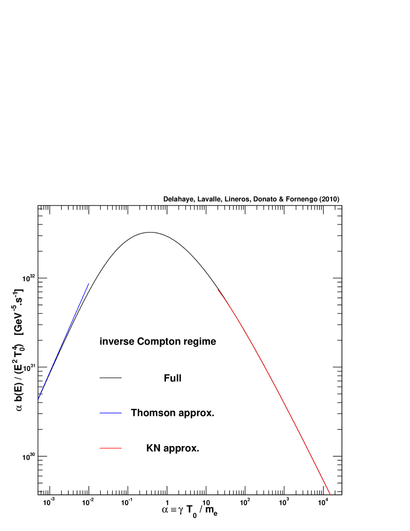
In the GeV-TeV energy range, electrons lose their energy by electromagnetic interactions with the ISRF (inverse Compton scattering) and the magnetic field (synchrotron emission), while Bremsstrahlung, ionization and Coulomb interactions with the ISM are negligible. Most studies have used the Thomson approximation to account for inverse Compton losses, which is valid for an electron Lorentz factor , where is the photon energy (e.g. Moskalenko & Strong 1998; Delahaye et al. 2009). This translates into a maximal electron energy of GeV for interactions with CMB ( eV), and of GeV for IR / starlight radiation, respectively (with eV). From those numbers, it is clear that the Thomson approximation is no longer valid for energies at Earth above a few tens of GeV, for which a full relativistic description of the term in Eq. (1) is consequently necessary. Few other studies have implemented this relativistic treatment (e.g. Kobayashi et al. 2004; Schlickeiser & Ruppel 2009).
The calculation of inverse Compton scattering of electrons with photons in the relativistic regime was derived in the astrophysical context by Jones (1965). It was subsequently extensively revisited and complemented by Blumenthal & Gould (1970). In the following, we rely on the latter reference to derive our relativistic version of the inverse Compton energy losses, to which we refer the reader for more details.
We consider relativistic electrons propagating in an isotropic and homogeneous gas of photons, which, moreover, exhibits a black-body energy distribution. The relevance of these assumptions will be discussed in Sect. 2.5. The electron energy-loss rate can be expressed in terms of the energies and of a photon before and after the collision, respectively, as
| (24) |
The collision rate is given by
| (25) |
where is the initial photon density in the energy range , which, for black-body radiation has the form (including the two polarization states)
| (26) |
and
| (27) |
From kinematics, the range for is readily found to be , which translates into for . It is convenient to rewrite the energy loss rate in terms of an integral over
| (28) | |||||
where the integral over is found to be analytical, so that one can easily check the full numerical calculation.
We define a dimensionless parameter that characterizes the relevant regime to be used for the energy loss rate
| (29) |
where is the mean temperature of the radiation field.
The non-relativistic Thomson limit is recovered for inverse Compton processes within a black-body radiation field, using or equivalently
| (30) |
where , whereas the Klein-Nishina regime applies for
| (31) |
In Fig. 1, we compare both regimes with the full calculation. From our numerical results, we derived a parameterization that is valid for any black-body radiation field, given by
| (32) |
where the conditions read
| (33) |
The fitting formula associated with the intermediate regime provided in Eq. (32) may be used with the parameters
| (34) | |||||
An additional smooth interpolation between these three regimes might improve the calculation by avoiding tiny gaps at connections, which could arise e.g. from very small numerical differences in the unit conversions or constants used above. This parameterization is valid for any black-body distribution of photons. If one considers a black-body distribution, the absolute energy density of which differs from that generally derived , then one can simply renormalize Eq. (32) by a factor to obtain the correct energy-loss rate.
In the following, we use Eq. (32) to describe the energy loss rates associated with Compton processes.
2.5 Review of the propagation parameters
In addition to energy losses, five parameters regulate the diffusion properties of Galactic CRs: and defining the diffusion coefficient (see Eq. 4), the half-thickness of the diffusion zone , the convective wind velocity , and the Alfvèn speed of magnetic field inhomogeneities , responsible for reacceleration. It was shown in Delahaye et al. (2009) that the last two effects can be neglected above a few GeV. These parameters were self-consistently constrained in Maurin et al. (2001) with ratios of secondary to primary nuclei — mostly boron to carbon B/C (see also Putze et al. 2010, for a more recent analysis). In the following, we use the available parameter space provided by these authors. Nevertheless, as useful beacons for bracketting the theoretical uncertainties, we also use the min, med, and max subsets of propagation parameters, which were derived in Donato et al. (2004) and called so after the hierarchy found on the primary antiproton fluxes, for sources spread all over the diffusion zone (not only in the disk). These models are described in Table 1.
For the normalization of the diffusion coefficient , we note that measurements actually constrain , not alone (Maurin et al. 2001). Moreover, using radioactive species does not allow yet to fully break this degeneracy (Donato et al. 2002). This explains why the min (max) configuration, which has a small (large) , is associated with a small (large) value of . The spectral index of the diffusion coefficient decreases from min to max, which is important to the spectral analysis of the electron flux.
| Model | |||||
|---|---|---|---|---|---|
| [kpc2/Myr] | [kpc] | [km/s] | [km/s] | ||
| min | 0.85 | 0.0016 | 1 | 13.5 | 22.4 |
| med | 0.70 | 0.0112 | 4 | 12 | 52.9 |
| max | 0.46 | 0.0765 | 15 | 5 | 117.6 |
Tighter constraints are expected to be possible with future PAMELA data, and hopefully with AMS2 (Battiston 2007). The current uncertainty in those parameters leads to large theoretical errors in secondary positrons (Delahaye et al. 2009) and therefore electrons, as reviewed in Sect. 3. The error in astrophysical primaries is assessed in Sect. 4.4
In contrast to stable nuclei in the GeV-TeV energy range, electrons are strongly affected by energy losses, which have a significant effect on their transport. It was shown in Delahaye et al. (2009) that inverse Compton and synchrotron processes dominate in this energy domain. Therefore, it is crucial to constrain the ISRF — including the CMB, and radiation from dust and stars — and the magnetic field as accurately as possible, within the horizon of GeV-TeV electrons, i.e. .
In Sect. 2.4, we developed a method to calculate the inverse Compton energy losses in a fully relativistic formalism, provided the target radiation fields can be described in terms of black-body distributions. This is obviously the case for the CMB, the temperature of which was recently re-estimated in Fixsen (2009) to be 2.72600.0013 K. However, it is well known that the ISRF is not simply Planckian radiation, since it consists of many different components — IR radiation from dust, optical and UV radiation from stars, diffuse X-ray emission, etc. — with different spatial distributions. Since by using CMB only we estimate the electron propagation scale to be 2 kpc for electron energies above 10 GeV, we disregard the spatial dependence of the ISRF, and only consider local averages.
In the left panel of Fig. 2, we report the ISRF data that we extracted from the analysis of Porter et al. (2008), and averaged in cylinders of radius and half-height of pc (model 2, M2) and kpc (model 1, M1) about the Earth, on top of which we show that a sum of black-body distributions can provide a reasonable fit. These two models, defined with a set of components characterized by their temperatures and energy densities, are summarized in Table 2. They can be used to estimate the theoretical error coming from uncertainties in the characterization of the ISRF. We may assume that these uncertainties reflect those affecting the data that we used, though error bars are not available. Note that the parameterizations appearing in Table 2 are not designed to reflect the true radiative physics operating in the ISM, which is beyond the scope of this paper. Nevertheless we observe an interplay between the IR and UV components, depending on the averaging volume: taking a smaller volume results in a larger (smaller) IR (UV) contribution due to the efficient UV-absorption and IR-emission properties of the dust, which is mostly concentrated in the disk.
| [K] | U [ GeV.cm-3] | ||
| CMB | 2.726 | Planckian (b-b) | |
| M1 | IR | ( b-b) | |
| Stellar | ( b-b) | ||
| UV | ( b-b) | ||
| ( b-b) | |||
| ( b-b) | |||
| M2 | IR | ( b-b) | |
| Stellar | ( b-b) | ||
| UV | ( b-b) | ||
| ( b-b) | |||
| ( b-b) |
The synchrotron emission can also be expressed as an inverse Compton scattering on a black-body distribution of virtual photons from the magnetic field. In this case, the characteristic energy of the radiation field is given by the cyclotron frequency
| (35) |
where is the electron mass, is Boltzmann’s constant, and is the value of the Galactic magnetic field. It is clear that the condition is fulfilled for the whole electron energy range considered in this paper, so that the Thomson approximation is fully valid. We estimate the local magnetic field relevant to the synchrotron losses to G (see e.g. Ferrière 2001), for which the corresponding energy density derived from classical electrodynamics is .
The synchrotron energy losses do not depend on the mean value of the magnetic field , but on the mean value of the squared field . Although the mean value , namely the regular component of the magnetic field, the irregular component implies that .
Jaffe et al. (2010) provide constraints on the different components of the magnetic field inside the disk. There are actually three components: the regular component and two irregular components (one aligned with the regular one , the other completely isotropic ). The relevant value we need for the synchrotron losses is
| (36) |
where it is easy to show that the variance is given by . (Note that ).
From the results obtained by Jaffe et al. (2010), we find that
| (37) | |||||
which translates into the range
| (38) |
Nevertheless, we should not neglect the vertical dependence of the magnetic field, which is usually found to be exponential, with a typical scale of 1 kpc. We emphasize that this scale is generally obtained from Faraday rotation measures as well as from observations of the all-sky polarized synchrotron emission, which translate into magnetic field intensity only after deconvolution of the thermal and non-thermal electron density. This density is usually grossly modeled by assuming the sum of Boltzmann and single-index power-law spectra, and a -exponential spatial dependence, which is itself motivated from radio observations of the same synchrotron emission (see Jansson et al. 2009, for a recent analysis). Therefore, these estimates might be affected by potentially large systematic errors.
We assume for simplicity that all components are constant in the disk (justified at the kpc scale around the Earth) and have the same vertical behavior, so that
If we average inside a spherical volume of radius 2 kpc, which corresponds to the typical propagation scale for electrons, we find that assuming that kpc. Given the range in Eq. (38), we obtain
| (39) | |||||
Using kpc is an extreme assumption, which is certainly not realistic. Nevertheless, assuming values in the range 1-3 G seems reasonable.
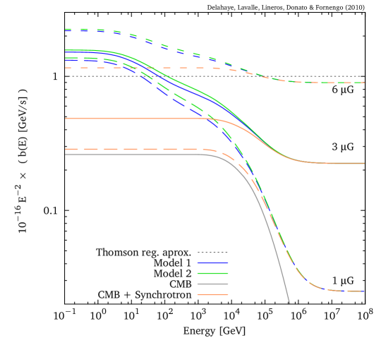
Therefore, although there are uncertainties in the local value of the magnetic field, we suppose G in the following, so that the ISRF model M1 complemented with the corresponding synchrotron losses leads to s in the Thomson approximation. The overall energy-loss rate is plotted in the middle panel of Fig. 2, where it is shown to differ from the Thomson approximation with s very often used in the literature, and which appears as the dashed straight line. In particular, we observe a cascade transition due to Klein-Nishina effects, where it appears that the loss rate index defined in Eq. (4) decreases step by step from 2, its Thomson value: at about 1 GeV, relativistic corrections become sizable for interactions with the main UV component which is felt less and less by electrons; then, across the range 10-100 GeV the IR component gradually loses its braking potential, and finally, above 10 TeV, interactions with CMB also cease. The value of the magnetic field sets the minimal value of the energy loss rate at higher energies. Since this latter is proportional to , varying from 1 to 3 G translates into additional order of magnitude in the energy-loss rate at high energy, as also depicted in the middle panel of Fig. 2; for completeness, we also display the case of taking 6 G. Note that considering CMB only provides a robust estimate of the minimal energy-loss rate, which converts into a maximal flux by virtue of Eq. (20); adding the synchrotron losses would instead define a next-to-minimal model for the energy losses.
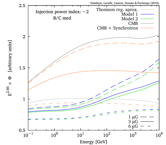
In the right panel of Fig. 2, we quantify the impact of using different energy-loss models to derive IS flux predictions, for which we adopt the med propagation setup and a template injection spectrum homogeneously distributed in a thin disk. The dotted curve corresponds to the Thomson approximation with s, where we recover a flux with predicted index , as predicted from Eq. (21) with . The higher curve is the flux obtained with the minimal case for the energy-loss rate (the minimal ), i.e. considering the CMB only, which provides the maximal flux. Indeed, in the Thomson approximation, the flux scales like , as seen from Eq. (20). The index reaches a plateau around in the range 10-1000 GeV, and then substantially hardens above 1 TeV because of relativistic effects. The next-to-minimal case exhibits the same feature, though the amplitude is slightly reduced, as expected. Finally, we report the flux associated with our complete models M1 and M2, both associated with a magnetic field of 1 G (short dashed curves), 3 G (solid curves), and 6 G (long dashed curves). We remark that the naive prediction of in the Thomson regime does not hold anymore, since the energy dependence of the energy loss is no longer equal to 2, and the observed spectral index is significantly harder. Indeed, we have to consider instead an effective value to account for relativistic effects. Taking a larger value of the magnetic field slightly softens the index and decreases the amplitude, as expected.
From this analysis of the local energy losses, we can estimate that the related uncertainties translate into a factor of in terms of IS flux amplitude (), and, above 10 GeV, in terms of spectral index (see the left panel of Fig. 2). Note, however, that this crude spectral analysis is valid for a smooth distribution of sources only, i.e. for secondaries. We see in Sect. 4.3 that considering discrete nearby sources of primaries strongly modifies this simplistic view.
3 Secondary CR electrons and positrons
We performed an exhaustive study of the secondary positron flux in Delahaye et al. (2009), which is qualitatively fully valid for electrons and to which we refer the reader for more details.
Secondary electrons originate from the spallation of hadronic cosmic ray species (mainly protons and particles) in the interstellar material (hydrogen and helium). This process produces also positrons, though different inclusive cross-sections come into play. Since spallation involves positively charged particles, charge conservation implies that it generates more positrons than electrons (e.g. Kamae et al. 2006). This statement is not entirely accurate for neutron decay, but electrons arising from neutron decay have a very low energy (mostly E 10 MeV), thereby out of the energy range considered in this paper. In sum, the steady-state source term for secondaries may in all cases be written as
| (40) |
where flags the CR species of flux and the ISM gas species of density , the latter being concentrated within the thin Galactic disk, and is the inclusive cross section for a CR-atom interaction to produce an electron or positron of energy .
For our default computation, we selected the proton-proton cross-section parameterizations provided in Kamae et al. (2006). Any nucleus-nucleus cross-section (e.g. or ) can be derived from the latter by applying an empirical rescaling, usually by means of a combination of the involved atomic numbers. However, this rescaling is found to be different for the production of and , or equivalently of and . We used the prescriptions from Norbury & Townsend (2007) for this empirical rescaling.
Fits of the proton and particle fluxes are provided in Shikaze et al. (2007), based on various measurements at the Earth. Finally, we employed a constant density for the ISM gas, with and , confining these species to a thin disk of half-height pc. This is summarized in cylindrical coordinates by
| (41) |
For this spatial distribution of the gas, the spatial integral of Eq. (19) can be calculated analytically, following Delahaye et al. (2009); the solution is reported in Sect. A.1. We underline that this approximation is locally rather good over the whole energy range as long as the true gas distribution does not exhibit too strong spatial gradients over a distance set by the half-thickness — this is discussed in more detail for primaries in Sect. 4.2. In any case, this estimate is more reliable at high energies ( GeV) for which the signal is of local origin independent of . At lower energies this approximation is expected to be valid for moderate kpc, but much less trustworthy for large-halo models, as in the max propagation setup. For these extreme configurations, a more suitable description of the gas distribution would be necessary.
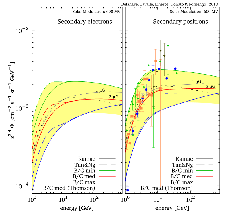
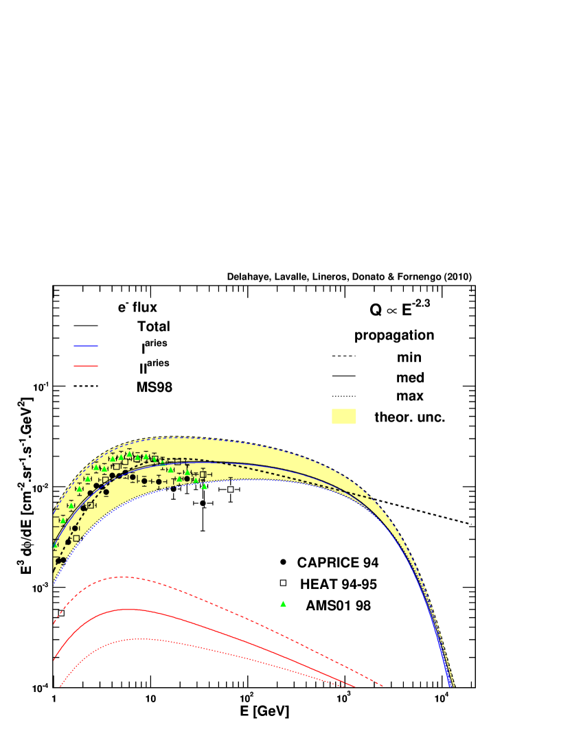
In Fig. 3, we plot our results for the secondary electron (left-hand side) and positron (right-hand side) fluxes at the Earth. For the solar modulation, we used the force-field approximation with a Fisk potential of MV (Fisk 1971). The solid curves are derived with the M1 ISRF model, a relativistic treatment of energy losses and nuclear cross-sections from Kamae et al. (2006). The yellow band is the flux range available for all sets of propagation parameters compatible with B/C constraints derived in Maurin et al. (2001). We observe that the min (max) configuration provides the highest (lowest) and softest (hardest) flux, among the three beacon models. This can be clearly understood from Eq. (20), since the min configuration is characterized by the weakest value of diffusion coefficient normalization associated with the strongest index , which is reversed in the max configuration. However, we recall that these models were named so for sources distributed all over the diffusion halo, not only confined to the disk as is the case here.
The discussion in Delahaye et al. (2009) on the theoretical uncertainties affecting secondary positrons is fully valid for secondary electrons. Aside from energy losses, errors may originate from either uncertainties in the light nuclei flux, or uncertainties in nuclear cross-sections, or both. The former can be evaluated by using different fits of the local measurements, and by retro-propagating the CR nuclei flux to account for potential spatial gradients. The latter may be estimated by considering alternative parameterizations of nuclear cross-sections. This is illustrated in Fig. 3 with the short-dashed curves computed with the nuclear cross sections of Tan & Ng (1983), which are shown to differ from our default model only at low energy below a few GeV. All these effects were studied for positrons in Delahaye et al. (2009) and lead to an uncertainty of about 40 %; this theoretical error is also valid for secondary electrons. Note, however, as we see later, that the electron flux is most likely to be dominated by the primaries, in contrast to positrons for which secondaries are a major component. Therefore, uncertainties in the secondary contribution has more impact for positrons than for electrons.
Finally, we emphasize that the present results differ slightly from those derived in Delahaye et al. (2009) because the energy losses are now treated in a fully relativistic formalism. Not only does this slightly change the normalization at low energy by a factor , but, more importantly, this hardens the spectral shape due to Klein-Nishina effects. This is more striking in Fig. 3, where the long-dashed curves are the predictions calculated in the med configuration and the Thomson limit for the energy losses. In Appendix B, we provide user-friendly fitting formulae that closely reproduce our calculations of the secondary electron and positron fluxes in the med propagation setup.
4 Primary electrons
The GeV-TeV CR electron flux at the Earth is dominated by a primary component originating from electrons accelerated in both SNRs and pulsar wind nebulæ(PWN) (Blandford & Eichler 1987). CR sources are therefore connected to the explosion of supernovæ(SNe), and we discuss a more general framework in Sect. 5. Predicting this primary contribution is a rather difficult exercise because it involves characterizing the energy distribution of these electrons at sources and their spatial distribution, in addition to their transport to the Earth. Moreover, since GeV-TeV electrons have a short range propagation scale, local sources are expected to play an important role. Rephrased in statistical terms, since the number of sources exhibits large fluctuations across short distances, the variance affecting the predictions is expected to increase with energy, when the effective propagation volume decreases. Therefore, fluctuations in the properties of local sources will have a strong impact. In contrast, the low energy part of the CR electron spectrum might be safely described in terms of the average source properties, namely a smooth spatial distribution associated with a mean injected energy distribution.
In the following, we estimate the primary flux of electrons and quantify the associated theoretical errors. More precisely, we wish to quantify the relative origin and impact of these uncertainties. To do so, we first discuss in Sect. 4.1 the spectral shape properties that we consider in the forthcoming calculations, focusing on SNRs for the moment (pulsars are discussed in Sect. 5, together with the primary positrons); available spatial distributions are presented in Sect. 4.2. Then we discuss the uncertainties associated with the modeling of a single source in Sect. 4.3. We finally discuss the primary flux and related uncertainties in Sect. 4.4, in which we make a thorough census of the local SNRs likely affecting the high energy part of the spectrum.
4.1 Spectral properties of SNRs and related constraints
Most SNR models (e.g. Ellison et al. 2007; Tatischeff 2009) rely on the acceleration of CRs at non-relativistic shocks (e.g. Malkov & O’C Drury 2001) and predict similar energy distributions for the electrons released in the ISM, which can be summarized as
| (42) |
The spectral index is usually found to be around 2 over a significant energy range (Ellison et al. 2007) — but to exhibit large variations at the edges — in agreement with radio observations. Gamma-ray observations suggest that the energy cut-off is greater than a few TeV (e.g. Aharonian et al. 2009b). These studies find rather similar indices for protons and electrons. Since protons of energy above a few GeV are barely affected by energy losses and have a long-range propagation scale, the proton spectrum measured at the Earth can provide information about the mean index at sources. Since , the index at source is therefore . With and in the range 0.5-0.7, one finds in the range 2.0-2.3, in rough agreement with theoretical predictions. We discuss complementary constraints from radio observations at the end of this subpart.
Aside from the spectral shape, sizing the value of the normalization is much more problematic. To describe a distribution of sources in the Galaxy, one usually assumes that the high energy electron injection is related to the explosion rate of SNe, so that we can suppose that is such that the total energy carried by electrons is given by
| (43) |
where is the SN explosion rate, is the kinetic energy released by the explosion, and is the fraction of this energy conferred to electrons. Since we are only interested in the non-thermal electrons, we assume that GeV. Note that the spectral index influences the normalization procedure sketched above. For a single source, the same expression holds but without — we discuss this case later on. For convenience, we further define the quantities
| (44) | |||||
which also helps us to discuss the normalization issue.
Constraining , , and , is a difficult exercise. The explosion rate of SNe is typically predicted to be a 1-5 per century and per galaxy (e.g. van den Bergh & Tammann 1991; Madau et al. 1998), which is consistent with observations (e.g. Valinia & Marshall 1998; Diehl et al. 2006). Nevertheless, SNe are of different types, and may thereby lead to different CR acceleration processes. About of SNe are expected to be core-collapse SNe (CCSNe), the remaining consisting of type 1a SNe (SNe1a). This is at variance with the statistics derived from observations, which identify a higher percentage of the more luminous latter type. CCSNe are often observed in star formation regions and spring from the collapse of massive stars , while SNe1a, produced by older accreting white dwarfs, are more modest systems, while being more widely distributed.
Explosions of CCSNe with masses can typically liberate a huge amount of energy, erg, % of which is released in the form of neutrinos when integrated after the cooling phase of the proto-neutron star (e.g. Burrows 2000; Woosley & Janka 2005; Janka et al. 2007). The total kinetic energy available from CCSN explosions, mostly due to the energy deposit of the neutrinos in the surrounding material, is about erg. CCSNe usually give rise quite complex systems characterized by SNRs beside (or inside) which one can find active neutron stars such as pulsars and associated wind nebulæ (PWN) — we focus on pulsars in Sect. 5. In contrast, SNe1a are much more modest systems, the explosions of which blast all the material away without giving birth to any compact object and release an energy of about erg, which is transferred entirely to the surrounding medium (e.g. Nomoto et al. 1984; Gamezo et al. 2003; Mazzali et al. 2007). It is interesting to remark that despite the quite different natures of CCSNe and SNe1a, both types feed the ISM with the same typical kinetic energy. Since we consider only SNRs in this part, we assume that erg in the following.
The fraction of SN energy conferred to electrons was studied in Tatischeff (2009), and found to be about . This result is rather independent of the exact values of the spectral index and the cut-off energy , but the theoretical error is still of about one order of magnitude.
At this stage, we emphasize that the theoretical uncertainty in already reaches about 2-3 orders of magnitude on average, which is quite huge and translates linearly in terms of flux.
For known single sources, it is possible to derive tighter constraints on the individual normalizations from observations at wavelengths for which electrons are the main emitters. This is precisely the case for the non-thermal radio emission produced by synchrotron processes, provided the magnetic field is constrained independently. The synchrotron emissivity associated with an electron source of injection rate is given by (Ginzburg & Syrovatskii 1965; Blumenthal & Gould 1970; Longair 1994)
| (45) |
where an average is performed over the pitch angle , and where the synchrotron radiation power is defined as
| (46) |
and , which is called the synchrotron peak frequency, corresponds to the average frequency of the synchrotron emission arising when an electron of Lorentz factor interacts with a magnetic field , and is , where is the cyclotron frequency. We note the parallel between the synchrotron process and the the inverse Compton process: for the latter, an initial photon of energy would indeed be boosted to . We could calculate the radio flux from the emissivity, but it is also interesting to derive a more intuitive expression, which actually provides a fair approximation (Longair 1994)
| (47) |
where we assume that the entire radiation is emitted at the synchrotron peak frequency , which links to . The distance from the observer to the source is denoted by . We remark that only the synchrotron part of the electron energy loss rate appears — we therefore assume that this is the most efficient process within the source — and that we neglect the possible reabsorption of the synchrotron emission. Since is the energy lost by an electron, it corresponds to the energy of the emitted photon, so the factor allows us to infer the number of photons.
This expression allows us to constrain by means of the source radio brightness , which is usually found in catalogs
We readily derive
| (49) |
which translates into
| (50) | ||||
We have just recovered the well-known relation between the radio index and the electron index, .
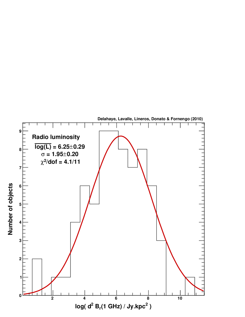
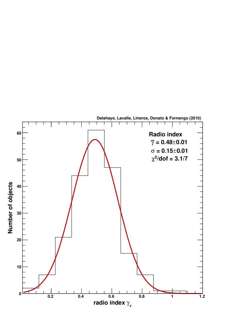
An up-to-date catalog of SNRs can be found in Green (2009), which contains 265 objects. Among these objects, only 70 have estimated distances to the Earth, and 207 have measured radio spectral indices. Observations, however, are not expected to reflect the actual statistical properties of the whole population of Galactic SNRs because of observational selection effects favoring the brightest sources and sites of fainter background (high longitudes, towards the anticenter). Disregarding the spatial distribution of these objects, which is probably strongly biased, this sample may still be fairly representative of their general spectral properties (Green 2005).
We compiled histograms of the measured radio indices and the estimated intrinsic luminosities — — in the right and left panels, respectively, of Fig. 4. The radio indices clearly appear to exhibit a Gaussian distribution, whereas luminosities follow a log-normal distribution. This points towards similar physical grounds for the electron properties at sources, which is obviously unsurprising. With these distributions, we can derive mean values and statistical ranges for the parameters. We find that and Jy.kpc2. One can therefore infer that the electron index in very good agreement with theoretical expectations. Although this relation between the radio index and the electron index is not entirely accurate (because of other radio components or absorption), and although some systematic errors also affect the data, this provides a complementary means of sizing the uncertainty, which is consistent with that of theoretical results.
We use this statistical information to directly constrain the single source normalization from Eq. (50), but we need to estimate the magnetic field in SNRs. From the observational point of view, information about the electron density and magnetic field at sources is degenerate. More insights may come from theoretical studies of the amplification of magnetic fields in sources from numerical simulations, which involve CRs themselves as seeds and amplifiers. The current state-of-the-art simulations (e.g. Lucek & Bell 2000) support G, in agreement with observations, and that we use here. With this value, we finally find for an index , which translates into (with a cut-off TeV). This is in rough agreement with the other values derived above, but probably biased, as expected, towards the brightest objects.
4.2 Spatial distribution of sources
Although GeV-TeV electrons have a short-range propagation scale, the injection rate of energy discussed above is insufficient to describe the Galactic CR electrons. We need to specify the spatial distribution of sources. For nearby sources, for which observational biased are less prominent, we can use available catalogs, which may provide a rather good description of the local CR injection. Nevertheless, for more distant sources, which have influence on the intermediate energy range 1-100 GeV, we have to rely on a distribution model.
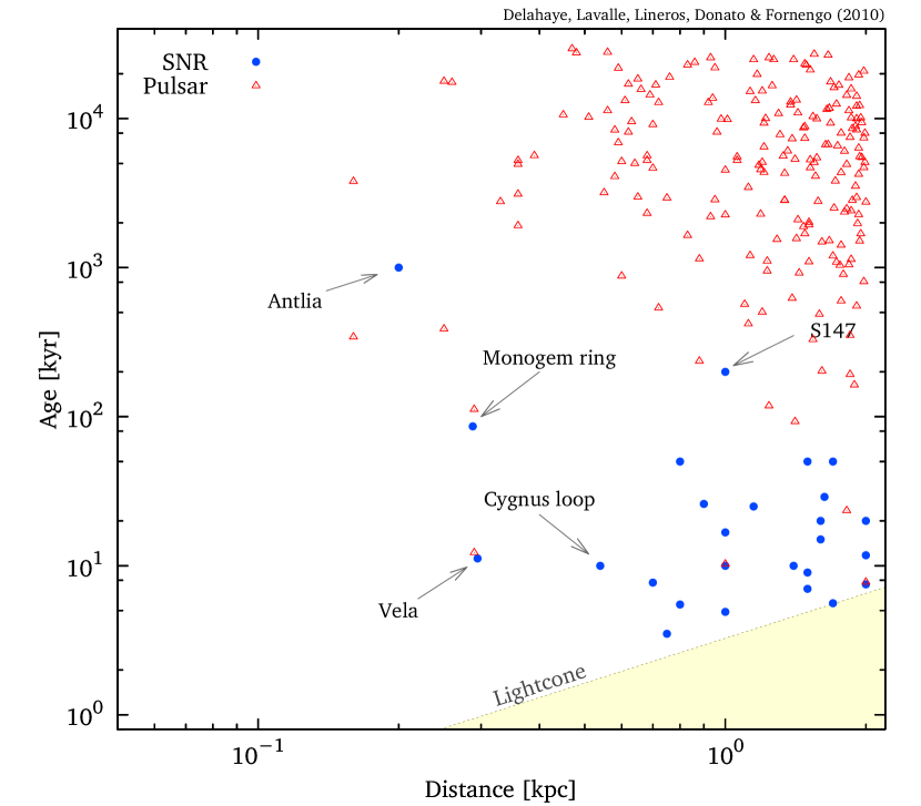
Since of SNe are expected to be CCSNe, one can use pulsars as tracers of the SNR distribution, instead of SNRs themselves, the observed population of which is much more modest. As an illustration, the ATNF catalog222http://www.atnf.csiro.au/research/pulsar/psrcat (Manchester et al. 2005) lists more than 1800 pulsars compared to the 265 SNRs contained in Green (2009). Nevertheless, a too naive use of the statistics would lead to errors since it is well known that data do not reflect reality faithfully because of detection biases (e.g. Lorimer 2004).
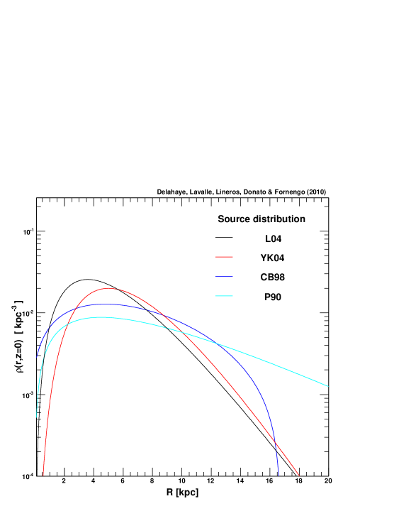
There are few distribution models available in the literature. Since the energetics associated with the source injection (birth) rate has been discussed above, we are only interested in the normalized source distribution here. Consequently, the normalization coefficient in front of each model is fixed such that it normalizes the spatial distribution to unity within the diffusion halo characterized by its radius and half-thickness . Moreover, in the following, we set the position of the Sun at kpc from the Galactic center333Some of the distributions listed in this paragraph are actually derived assuming 8.5 kpc, but we disregard this small change to make the discussion easier..
Most of models have radial and vertical dependences of the form
| (51) |
where ensures the normalization to unity. For simplicity, we discuss only differences of the radial distributions in the following, since the vertical distribution is fairly similar among studies. We thereforee keep fixed the vertical dependence as in the above equation, with kpc, throughout the paper.
Different sets of values can be found in the literature for the pair . Lorimer (2004), hereafter L04, found ; Yusifov & Küçük (2004), hereafter YK04, derived ; while Paczynski (1990), hereafter P90, early determined . Finally, in contrast to the parameterization sketched above, we recall the distribution proposed by Case & Bhattacharya (1998), hereafter CB98, though it was obtained from a fit to data of poor statistics for 36 SNRs
| (52) |
where we have added the same vertical term as in Eq. (51). The authors found kpc, kpc, and . This relation is only valid for , i.e. within 16.8 kpc, and null beyond. Note, however, that Brogan et al. (2006) reported the detection of 35 new remnants in the inner Galaxy, and suggest that former radial distribution estimations should be revised.
To understand the deviations induced in the electron flux prediction when using these different distributions, it is convenient to define the following halo function
| (53) | ||||
which determines the probability of an electron reaching the Earth given its propagation scale — see Eq. (3) — and the normalized spatial distribution of source . The electron flux is the the energy integral of the product of this probability and the source spectrum, such that the shape of this probability function provides a preliminary taste of the final result. More importantly, it allows us to connect the spatial origin of the signal with energy, through the propagation scale .
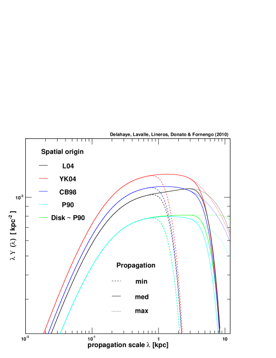
In the left panel of Fig. 5, we plot the spatial distributions listed above as functions of the galactocentric radius , and in the galactic plane (). We see that except for the solar neighborhood, where relative amplitudes can vary by a factor of 2 at most, the spatial distributions in the direction of the Galactic center and towards the anticenter are quite different from each other. Nevertheless, these differences are significantly lower in terms of , because of the spatial average — see Eq. (53). This is shown in the middle panel of Fig. 5, where we have plotted as a function of for the different spatial distributions and for the min, med, and max propagation setups. We see that the probability is maximal and constant — grows linearly with — for short propagation scales up to kpc. Then, the probability decreases linearly with — exhibits a plateau — before shrinking exponentially when , being larger and larger from the min setup to the max setup. Each spatial distribution model is characterized by a very similar curve that differs mostly in terms of amplitude. This can be understood in the following manner: when , the source can be considered as homogeneous in 3D space, then ; when , since the source distributions do not exhibit strong radial variations on the kpc scale, they can be considered as thin disks, and one recovers the solution derived in Eq. (20); for , electrons escape the diffusion zone. This points towards the possibility of modeling, while only locally, the source distribution with a z-exponential infinite disk, for which full analytical solutions of the spatial integral exist. The green curve in the middle panel of Fig. 5 is the z-exponential disk approximation associated with P90, as an illustration, and is shown to provide a rather good approximation except for large diffusion thickness kpc. The z-exponential disk approximation is defined in cylindrical coordinates as
| (54) |
where is the local value of the normalized density given in Eq. (51). This approximation is valid for local predictions provided the spatial distribution does not vary significantly over a distance , which is the case for moderate . In the right-hand side panel of Fig. 5, we compare the disk approximation with the full calculation in terms of fluxes: for different spatial distributions, we plot the ratio approximated flux / exact flux for our three beacon propagation setups. We can see that the exponential disk approximation is quite good above a few GeV for the min and med cases, as expected, having an accuracy better than 5%. Errors are obviously larger in the max case because of the larger spatial gradients exhibited by the spatial distributions within kpc.
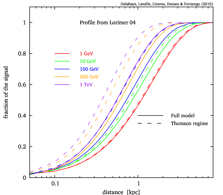
A final useful exercise regarding the smooth spatial distribution modeling consists of checking the cumulative fraction of the IS signal received at the Earth as a function of the radial integration distance. In Fig. 6, we report this fraction for spatial model L04 at different energies, assuming an injection spectrum , and for both the Thomson approximation and the relativistic energy losses. We see that this fraction increases more quickly at high energy than at low energy, as expected from energy losses. This is consistent with the result obtained in Delahaye et al. (2009) for secondary positrons. Nevertheless, above 10 GeV, we can observe that relativistic effects come into play and a difference appears between the Thomson approximation case and the relativistic case. Indeed, the latter induces a longer propagation scale at high energy, and consequently softens the rise of the cumulative fraction. This would be slightly less significant for a magnetic field of 3 G instead of 1 G, though still observable.
Another important piece of information that we can derive from Fig. 6 is that the cumulative signal fraction is (80%) for kpc and (10) GeV. This helps us to define consistent means of including local sources in our predictions, as we discuss later in Sect. 4.4.2. Indeed, we know at present that if we replace the smooth spatial distribution within 2 kpc with discrete sources, these latter can affect the whole available energy range quite significantly: if powerful enough, local sources will dominate above a few tens of GeV, otherwise, flux predictions will be significantly depleted compared to a smooth-only description of sources, for a given normalization pattern.
4.3 Sizing the uncertainties for local sources
Before discussing the contribution of local known SNRs to the CR electron flux (see Sect. 4.4.2), it is essential to review the impact of uncertainties in the main parameters describing the source. They are only a few, but their effects on the flux are shown to be important and degenerate.
Apart from the propagation modeling and related parameters that were presented in Sects. 2.2 and 2.5, theoretical errors may originate from uncertainties (i) in the spectral shape and normalization, (ii) in the distance estimate, (iii) in the age estimate and (iv) in our understanding of the escape of cosmic rays from sources. The last point is actually still debated and poorly known in detail (see e.g. Caprioli et al. 2009), though it is clear that the release of cosmic rays in the ISM is a time- and energy-dependent process which takes place over yr, i.e. the lifetime of the source. Since this timescale is still almost always much lower than the diffusion timescale, Myr for distances in the range 0.1-1 kpc, we ignore the dynamical aspects of injection in this study, while we stress that they may lead to sizeable effects, especially in the case of very nearby sources. The first point was discussed in Sect. 4.1, and is featured by two main parameters: the spectral index at source and the energy released in the form of high energy electron , both related in the normalization procedure given Eq. (43) that allows to derive . Points (ii) and (iii) have some impacts that can be understood from Sect. 2.2 and Sect. 2.3. Although the consequences of varying these parameters can be understood from equations only, we aim here to illustrate them in a more pedagogical way. To do so, we will consider a template event-like source located in the Galactic plane () at a distance to the Earth and bursting a population of electrons a time (age) ago:
| (55) |
where the spectrum is given by Eq. (42). We will assume here that erg. Note that, as emphasized in point (iv) above, a more realistic source term would not involve a burst-like release of electrons in the ISM at time , but instead a more complex time-dependent energy spectrum. Such refinements are beyond the scope of this paper.
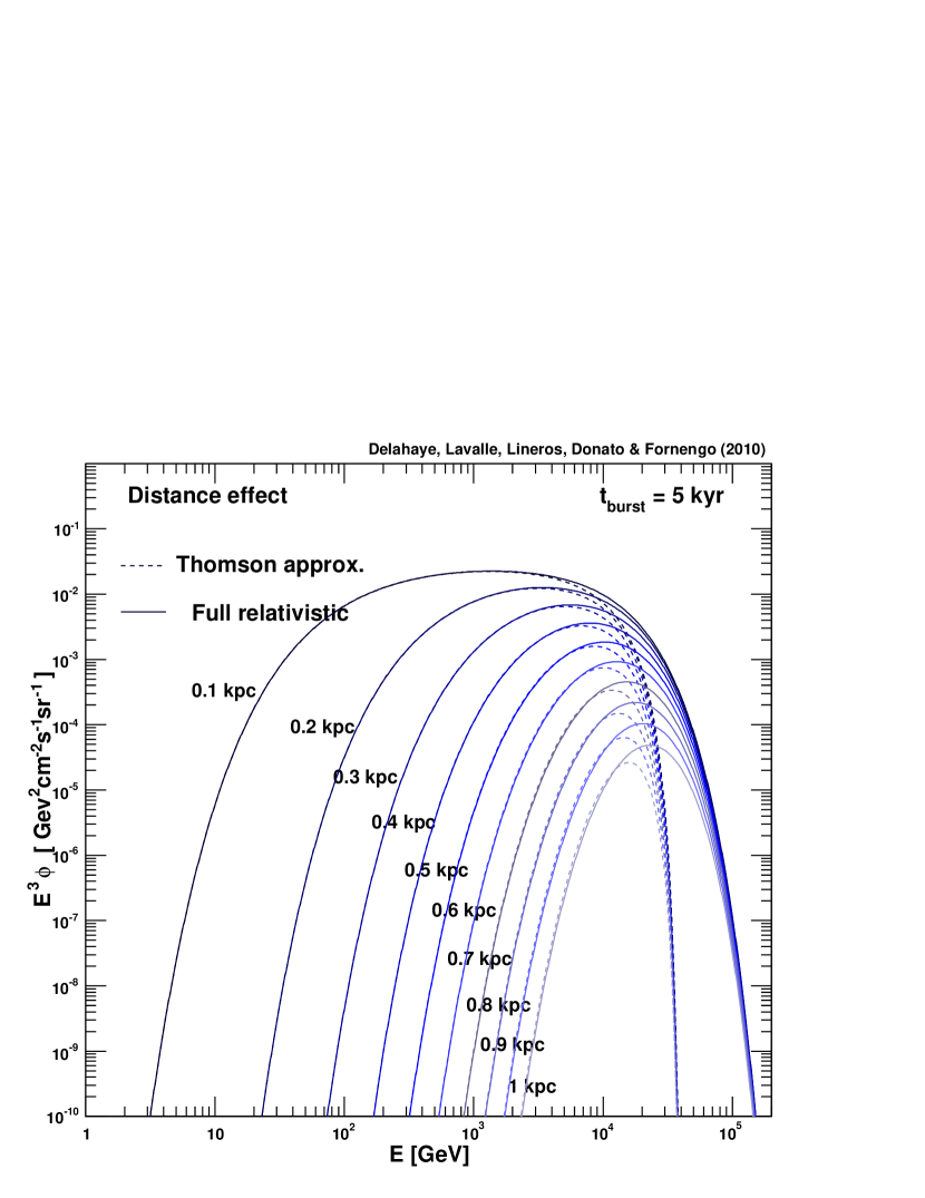
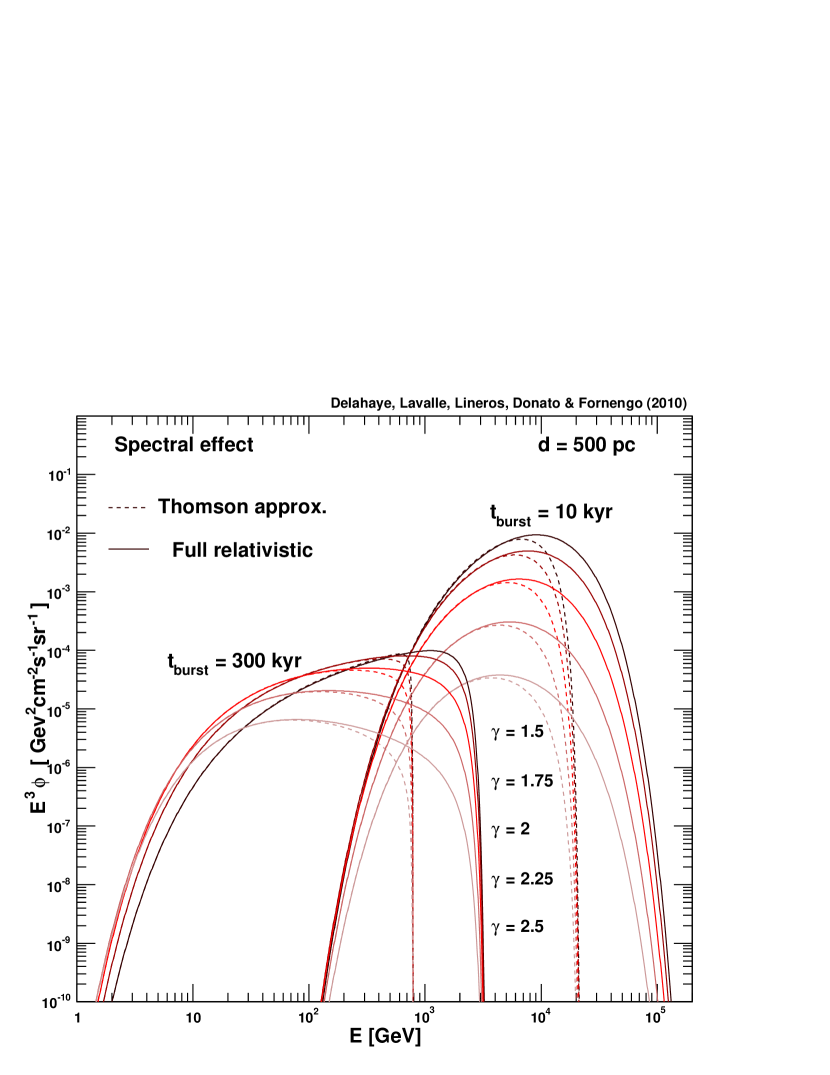
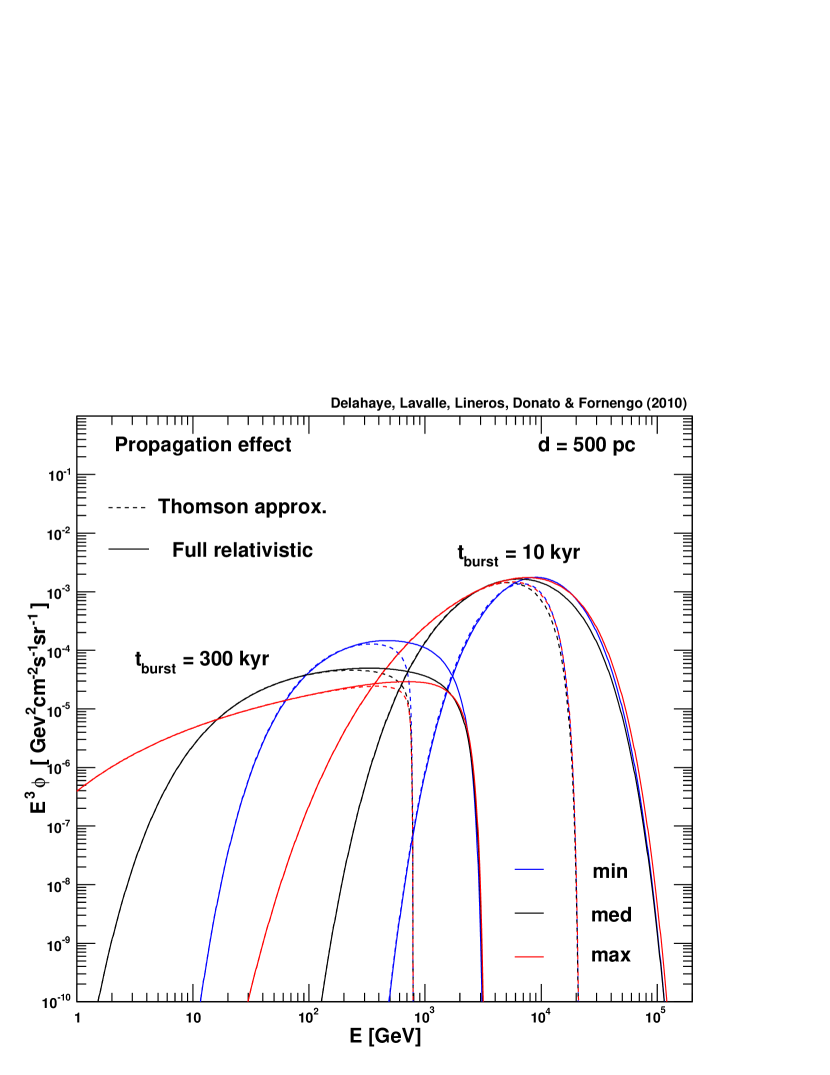
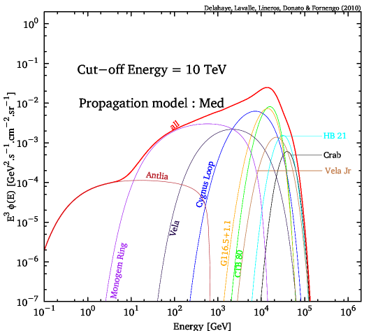
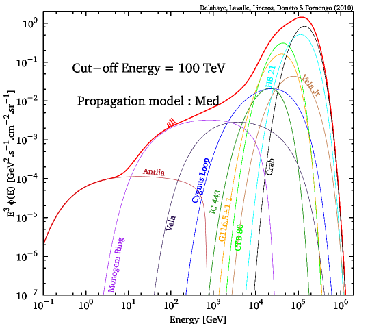
In Fig. 7, we plot the electron flux for different configurations of the parameters, the default configuration being defined by: med, , TeV.
In the top left panel (a), we show the source age effect; in the top right panel (b), we illustrate the distance effect; in the bottom left panel (c), we sketch the spectral index effect; while in the bottom right panel (d), we plot the propagation model effect. For all panels, we report the fluxes calculated in both the Thomson approximation and the full relativistic treatment of the energy losses, as discussed in Sects. 2.4 and 2.5.
As a first comment, we emphasize that the Thomson approximation can lead to a very strong under-estimate of the spectral break inferred from energy losses, up to one order of magnitude in the examples shown. This is a mere consequence of the over-estimate of the energy loss rate at high energy. The net effect obviously depends on the magnetic field and on the actual cut-off considered at the source. As regards the latter, we see that using a value of 10 TeV already induces an underestimate by a factor of 5-10 of the break predicted in the non-relativistic regime. Many studies of the topic have employed the Thomson approximation.
The second important comment to make is that it is actually quite difficult to relate the observed spectral index to the source spectral index, because of the complex and degenerate effects coming from all parameters: distance, age, source index, energy cut-off, normalization and diffusion coefficient. For instance, we see that a large diffusion coefficient (min model) can make a source of 300 kyr resemble a source of 30 kyr associated with a larger diffusion coefficient and a lower energy cut-off. In any case, a mere glance at the four panels of Fig. 7 is striking enough.
This exhaustive analysis of the impact of the main parameters characterizing individual sources already points towards the difficulties that we encounter in the interpretation of the data. Nonetheless, although this part might look depressing at first sight in the perspective of making predictions, it is still very useful to estimate the theoretical confidence level of our forthcoming attempts.
4.4 Primary electron flux and theoretical uncertainties
In the previous parts of this section, we have discussed the main physical quantities relevant for predictions of the primary electron flux at the Earth, emphasizing their role as potential sources of uncertainties. Here, we implement the full calculation and compare our results with available data on the electron flux. We stress that pure electron data are not numerous and rather old, since most of recent experiments either do not distinguish electrons from positrons or have not yet released their charge-discriminating data. We therefore only use the electron data from CAPRICE (Boezio et al. 2000), HEAT (DuVernois et al. 2001), and AMS-01 (Alcaraz et al. 2000), to avoid any confused interpretation mixing positrons. The pure positron case and the full case are discussed in Sects. 5 and 6, respectively.
We first compare the predictions arising from a smooth description of sources, for which we adopt the L04 spatial distribution. Indeed, we demonstrated in Sect. 4.2 that using different spatial distributions causes only small differences in the overall flux normalization locally.
We then estimate the contributions of all known local SNRs that can be added to a smooth and more distant component, following the method proposed in Kobayashi et al. (2004).
4.4.1 Smooth description of sources
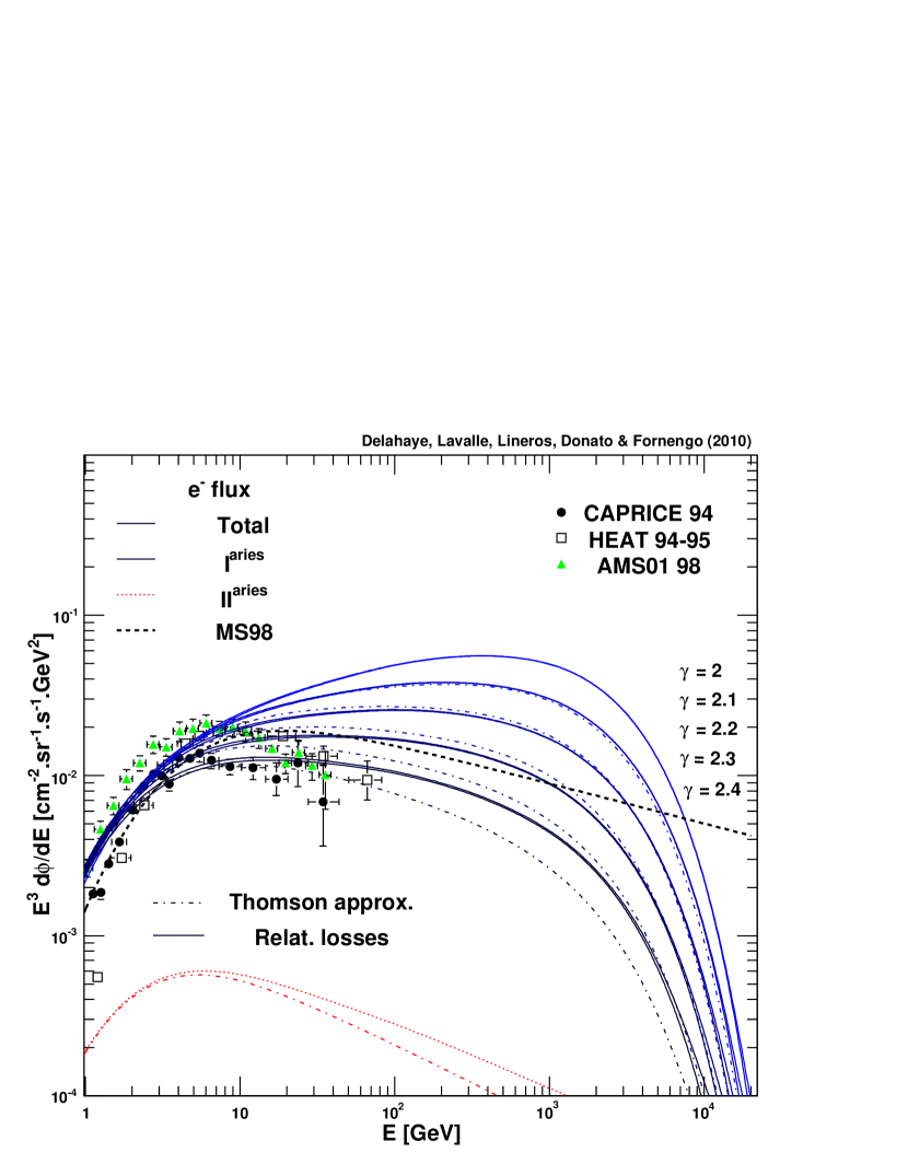
Our model for a smooth distribution of SNRs includes a propagation setup, a spatial distribution (here L04) and an injected spectrum, and it is interesting to check some of the possible configurations against the data. In particular, we attempt to constrain the injection normalization necessary for a model to fit, at least roughly, the data. For the spectrum, we test different spectral indices, but keep the energy cut-off at 3 TeV. As a reference normalization, we use a SN explosion rate of 4/century, a SNR total energy of erg, of which a fraction of is carried by electrons, giving therefore erg/century.
In Fig. 8, we report various flux calculations, for which we applied a solar modulation correction with a Fisk potential of 600 MV. In the left panel, we show the effect of varying the injected spectral index from 2 to 2.4 for the med propagation setup, using both the Thomson approximation and the relativistic regime for the energy losses. In this plot, we have renormalized by a factor of 5 for all indices, so that we see that reasonable fits to the data can be obtained within the expected normalization range discussed in Sect. 4.1. This means that the expected energy budget available for electrons is in rough agreement with what is needed to explain the current observations. From the same plot, we could also conclude that the injection spectral index should be slightly softer than 2. Nevertheless, this also depends on the logarithmic slope of the diffusion coefficient, as seen from Eq. (21) — complementary constraints on could also be derived from high energy proton data, based on the assumption that the proton index is the same as the electron index after their acceleration at sources and that proton propagation is simply described by diffusion (i.e. neither reacceleration nor convection). This is illustrated in the left panel of Fig. 8, where we show the effect of the theoretical uncertainties in the propagation parameters, using the same spectrum normalization and the same spectral index for all models. We see that the min model gives the larger amplitude because of its smaller value of and the softer observed index due to its larger diffusion slope (see Table 1 and Eq. (20)) — the analysis is reversed in the max configuration. For a given normalization, the amplitude uncertainty is therefore proportional to , which gives a factor of from the min to the max configurations. In both panels of Fig. 8, we also report the prediction obtained in Moskalenko & Strong (1998), as fitted in Baltz & Edsjö (1998), where the authors used an injection index of 2.1 below 10 GeV, steepening to 2.4 above. This model, very often quoted as a reference model, is shown for comparison.
It is noteworthy that since the data have a quite limited statistics and range up to GeV only, they are probably insufficient to provide strong constraints on the electron cosmic ray component. Moreover, we recall that this smooth description of the SNR contribution is not valid locally above a few tens of GeV, where we expect discrete effects to become important. Nevertheless, this preliminary analysis is still useful to delineating the relevant ranges of the spectral index and the injected energy. Likewise, it helps us to determine the influence of distant sources relative to local ones.
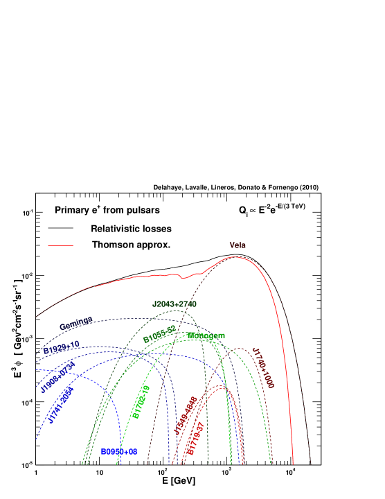
Finally, we emphasize that we only considered a single contribution from a SNR population. Nevertheless, the electron-positron pair injection from pulsars is also likely to account for a significant additional contribution to the local electron budget. It is not clear whether this contribution should have the same spectral index, and one could for instance model the smooth electron component with a combination of two spectral components, leading to an additional freedom in the normalization procedure. This electron component from pulsars is discussed in Sect. 5.
4.4.2 Contributions from known local sources
| 1 TeV | 10 TeV | 100 TeV | ||
| min | 5, 20, 22, 24 | + 23 | +8, 18, 19, 26 | |
| 5, 20, 22, 24 | +8, 18 | + 17,19 | ||
| 5, 20, 22, 24 | +8, 17, 18 | + 19 | ||
| med | 5, 20, 22, 24, 26 | + 4, 11, 19 | +8, 18, 23 | |
| 5, 11, 20, 22, 24 | +4, 8, 18,23 | + 19 | ||
| 5, 11, 20, 22, 24 | +4, 18, 19, 23 | + 8, 17 | ||
| max | 5, 20, 22, 24, 26 | + 8, 11, 19, 23 | +4, 18 | |
| 5, 20, 22, 24 | +8, 11, 18, 19 | + 4, 23, 26 | ||
| 5, 20, 22, 24 | +8, 11, 18, 19 | +4, 23, 24 |
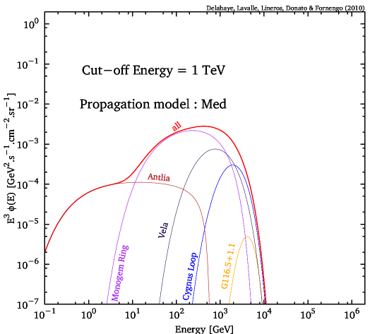
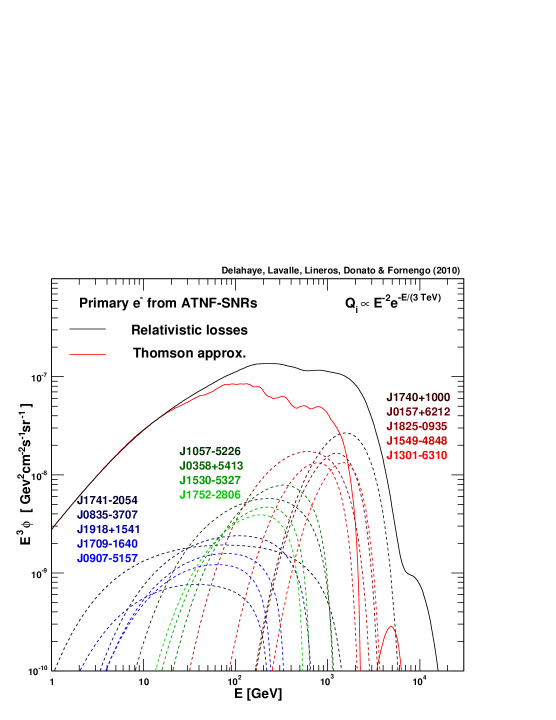
As discussed earlier, contributions from local sources are expected to be significant above a few tens of GeV. Following the method proposed in Kobayashi et al. (2004), we take a census of all known sources of primary electrons located within 2 kpc from the Earth in order to compute their associated flux explicitly.
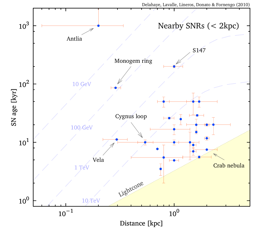
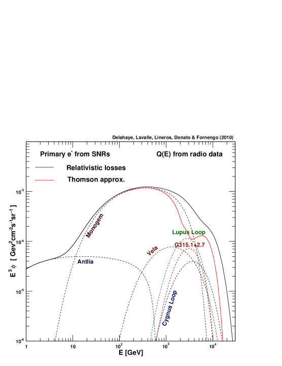
To proceed, we first took advantage of the information provided in the SNR catalog of Green (2009), and we performed an extensive synthesis of all published properties and associated errors (mostly from radio data). We found 26 SNRs within 2 kpc in this catalog, to which we added an extra-object, Antlia SNR (McCullough et al. 2002; Shinn et al. 2007). A full description of these sources including information about distance, age, spectral index, radio flux, associated objects, and bibliographic references is available in Appendix C. These properties are summarized in Table 6.
The event-like contribution of a single source is readily computed from the results obtained in Sect. 2.2. As a word of caution, however, we stress that the time argument used to feed the time-dependent propagator given in Eq. (18) should not be the observed age of the object given in catalogs, but instead the actual age, equal, in principle, to the observed age plus . Indeed, most of the age estimates depend on the dynamical properties of the objects inferred from multiwavelength observations, which correspond to the properties the object had a time ago. For the injection spectrum, we utilize Eq. (42) and set the spectral index from the observed radio index — . We constrain the spectrum normalization with the observed radio flux using Eq. (50).
Although SNRs are expected to provide an important contribution to the primary electron flux, we emphasize that pulsars are also expected to produce and accelerate electron-positron pairs. Modeling the electron injection from pulsar is discussed in more detail in Sect. 5, to which we refer the reader. We found that pulsars located within a distance of 2 kpc from the Earth could contribute to the local electron budget, among which few may be dominant (see Sect. 5.2). For consistency reasons, we have to include the contribution of these pulsars to the electron flux.
An additional important remark should be made about the non-observed local sources of primary electrons that should exist. So far, we have listed 27 SNRs and about 200 pulsars. Nevertheless, we recall, as we discuss in more detail in Sect. 5, that pulsars are rotating neutron stars originating from core-collapse supernova explosions. Therefore, each pulsar should be accompanied by a SNR. Such a systematic association is obviously not supported by observations. This is already illustrated in our object list, in which we find only 27 SNRs for 200 pulsars. Among these 27 local SNRs, only 10 have a known pulsar counterpart (very often with differences in their distance and age estimates). However, this certainly does not mean that the theoretical expectation is wrong, since not all SN explosions lead to pulsars, but instead that the counterparts are probably not bright enough to be observed. Therefore, again for theoretical consistency reasons, we choose here to add a SNR counterpart to each non-associated pulsar, but with a brightness such that it could not be observed with current telescopes. We adopted as a general criterion for non-observed SNRs. These local statistics can be tested against predictions of the SN explosion rate . If we assume at zeroth order that sources are distributed homogeneously inside a flat disk of radius kpc, then the local explosion rate within a radius of kpc around the observer is given by , leading to 0.01 SN/century for usual values of . This can be compared with the observed local explosion rate, which we can estimate from the number of sources in our sample divided by the oldest age, i.e. . This rough calculation leads to a difference of only a few, which would tend to tell us that using only the observed sources translates into a slight underestimate of the actual local electron budget. This makes sense, since observations favor the brightest objects, and also since rapidly-rotating magnetized neutron stars with magnetic axes pointing away from the Earth cannot be observed as pulsars. Our samples of local SNRs and pulsars are shown in the age-distance plane in Fig. 9.
In Fig. 10, we show the electron flux obtained in the med propagation setup, using the local SNR properties summarized in Table 6 and assuming different cut-off energies. The first important comment to make is that the whole flux is far from being described simply by a smoothly injected power law, since many spectral wave-like features are evident. Moreover, because of the interplay between the age and the maximal energy (see Sect. 2.2), we see that varying the energy cut-off from 1 to 100 TeV, though the latter value is probably not realistic and too high, has considerable effects; not only do new contributions arise at high energy when the cut-off value increases, but the hierarchy among other sources is also altered. This illustrates an additional source of theoretical uncertainty, beside those we discussed in Sect. 4.3. Figure 11 illustrates the theoretical and observational uncertainties affecting both the source modeling and the propagation modeling. The left panel allows us to quantify the impact of the observational uncertainties on the ages, distances, radio fluxes and spectral indices. This plot portrays the results of 1,000 Monte Carlo realizations in which we drew each parameter according to a flat distribution within the observational errors. The right panel exhibits (i) the impact of varying the propagation parameters on the overall local SNR contribution and (ii) the differences associated with different injection spectrum prescriptions. For the latter point, we compared the flux obtained with generic spectral properties, namely a spectral index of 2 and a fixed normalization of (see end of Sect. 4.1), with the observationally constrained predictions. We again see that the global spectral shape is far more complex than a mere power law, and that the overall flux can vary within a factor of 2-5 depending on the energy.
We plot the results obtained with a template calculation for all local electron primaries in Fig. 12, where we used the med propagation setup with the M1 ISRF model (the large difference between the full relativistic calculation and the Thomson approximation is evident in the plots). The three panels from left to right show the contributions of local known SNRs, from non-observed SNRs associated with observed pulsars, and from observed pulsars, respectively. For the non-observed SNRs, we considered the distances and ages of the associated pulsars, and we assumed an injection spectrum with an index of 2 and a non-observable radio flux of . While the contribution from the non-observed SNRs is shown to be negligible with respect to the two others, it is interesting to note that our local pulsar modeling leads to a higher primary electron flux than local SNRs. For pulsars, we supposed than 10% of the spin-down energy was converted into electron-positron pairs when defining the individual normalizations (see Sect. 5). Although the injection mechanism is subject to large theoretical uncertainties, it is still rather surprising to find that even when accounting for observational constraints for pulsars, their local population can contribute as many primary electrons as known local SNRs. However, these calculations are subject to very large theoretical uncertainties, so no strong conclusions should be drawn: by no means should they be considered as predictions, only trends. The main conclusion at this stage is that nearby sources dominate the flux above energies of few tens of GeV, the spectral imprints of which are very difficult to predict, because of large theoretical uncertainties in their modeling. Finally, it is clear from the plots that the Thomson approximation can lead to large errors in the predictions.
4.4.3 Electron flux: sum of distant plus local sources
We can now derive a full calculation including all known local sources within a distance of 2 kpc from the Earth and a more distant smooth component. For the latter, we use the L04 spatial distribution, but in contrast to what we did in Sect. 4.4.1, we have to apply a radial cut-off to this smooth contribution within 2 kpc to the Earth, to avoid a possible double counting of the local sources. This means that the distant component has more impact at low energy than at high energy.
Furthermore, we can also compare our results with the available observational data about electrons. The top left panel of Fig. 14 shows an example of a calculation including all the components discussed above in a self-consistent manner, using the med propagation setup. To proceed, we fixed the entire parameter set from available observational constraints, and we tuned the other parameters to provide rough agreement between the calculated flux and the data. In particular, we adjusted the global normalizations and spectral indices of the two distant smooth components (one for SNRs, another for pulsars) and of the local pulsars. The parameters that we used are summarized in Table 5.
5 Primary positrons
The increase in the positron fraction inferred from the PAMELA data is barely consistent with what is expected for secondary positrons (e.g. Delahaye et al. 2009), except for those secondaries produced and accelerated in sources (Berezhko et al. 2003; Blasi 2009; Mertsch & Sarkar 2009; Ahlers et al. 2009). Additional spatial arguments might still be helpful in dealing with this issue (Shaviv et al. 2009).
Although exotic primary contributions from dark matter annihilation could contribute to the positron budget, the most popular dark matter particle candidates can hardly exceed the secondary background unless the annihilation rate is boosted substantially (e.g. Baltz & Edsjö 1998; Lavalle et al. 2008a; Delahaye et al. 2008; Bergström et al. 2008), or the expansion rate is more rapid than expected in the early universe, before the primordial nucleosynthesis (see Salati 2003 for the original idea, and e.g. Catena et al. 2009 more specifically for the positron channel). Furthermore, the potential enhancement provided by dark matter substructures was demonstrated to be too small (see Lavalle et al. 2008b, a; Pieri et al. 2009), and any other type of global enhancement was shown to be severely restricted by the companion upper limit to the antiproton yield (e.g. Donato et al. 2009), which fully applies to the most popular dark matter models that have in no case exclusive couplings to leptons. We therefore emphasize that generic dark matter candidates are not expected, unfortunately, to manifest themselves in the positron spectrum in the GeV-TeV energy range.
For other potential sources of primary positrons, we note that since the seminal work on electron-positron pair production in strong magnetic fields by Erber (1966), a particular class of cosmic-ray sources has long been predicted to provide electron-positron pairs: pulsars (Sturrock 1970, 1971). Interestingly enough, a detailed discussion about the increase in the measured positron fraction and the potential role of pulsars was already conducted two decades ago by Boulares (1989)444Boulares (1989) did also mention that dark matter was another, though exotic, possibility.. Subsequent deeper studies have been performed since then (e.g. Aharonian et al. 1995; Atoyan et al. 1995; Chi et al. 1996), which were recently revisited by several authors (e.g. Hooper et al. 2009; Profumo 2008; Yüksel et al. 2009; Malyshev et al. 2009). Since pulsars are commonly observed in the vicinity of the Earth, it is very likely that these astrophysical sources of positrons are the origin of most of the local cosmic ray positrons. Nevertheless, many uncertainties remain in the characterization of pulsars, and there has been little theoretical progress in the past decade.
Pulsars are rapidly-rotating magnetized neutron stars, the rotation axis of which is misaligned with the axis of the magnetic field, which produces a pulsed emission for an observer located on the cone scanned by the magnetic axis. They are potential end products of CCSN explosions, such as black holes for the most massive progenitors and other neutron stars unseen as pulsars (if the observer is always off-magnetic axis, the rotation and magnetic axes are aligned, or the neutron star is either non-rotating or non-magnetized). All pulsars must in principle be associated with a companion SNR. This is supported by observations since pulsar wind nebulae (PWNe) are sometimes found inside or close to the shells of SNRs (see e.g. Gaensler & Slane 2006; Bucciantini 2008, for recent reviews on PWNe), though many pulsars remain non-associated555Pulsars are likely usually expelled from the SNR system, but the relative velocity between both objects km/s induces a distance pc between them by the SNR lifetime. This distance may be larger for old systems, which makes clear associations more difficult.. Thus, a more general picture of pulsar modeling, at least for cosmic-ray electrons and positrons, should involve a SNR as the main energy supply, and a pulsar and its PWN as a subsystem injecting additional high energy electrons and positrons (see e.g. Blondin et al. 2001). Note that even though a SNR should be associated with each pulsar, the reverse is not true: explosions of SNe1a leave no compact objects at all, and some CCSNe do not become pulsars. Likewise, we stress that the cosmic-ray acceleration mechanisms are different in SNRs and in PWNe, leading to different observational properties. In the former case, acceleration takes place at non-relativistic shocks, while at relativistic shocks in the latter case, which might imply different spectral shapes for the accelerated electrons. Moreover, pulsars convert a significant part of their spin-down energy into electron-positron pairs that are accelerated by the PWNe; this does not occur inside SNRs, where the energy fraction transferred to electrons is much lower (see Sect. 4.1).
In this section, we complete our calculations of the electron and positron flux at the Earth by including the contribution of pulsars. We adopt the same methodology as for SNRs, and consider two populations, (i) the local one, for which we constrain the individual properties from observational data, and (ii) a more distant and smoothly described population. As in most recent studies, the individual properties of pulsars are derived from the ATNF catalog (Manchester et al. 2005). In Sect. 5.1, we sketch the generic model that we have adopted. In Sect. 5.2, we discuss the contributions of both populations to the local electron and positron flux. We then compare some template calculations to the current measurements of the positron fraction in Sect. 6.2.
5.1 Generic pulsar modeling
Independently of the specific pulsar model, such as for instance the polar gap (Ruderman & Sutherland 1975), the outer gap (Cheng et al. 1976, 1986), or the slot gap (Harding et al. 2008) models, we may summarize the physics relevant to the production of cosmic-ray electrons and positrons as follows. Gamma rays can be generated in the pulsar magnetosphere from inverse Compton interactions of electrons accelerated along the strong and rotating magnetic field with local synchrotron radiation, which can in turn produce electron-positron pairs by annihilating with photons from the local radiation fields. Those gamma rays can be observed as pulsed emission, such as those recently detected with the Fermi satellite (Abdo et al. 2009a), which may therefore be used to constrain the pair production. These electron-positron pairs are then accelerated within the surrounding and expanding shocked medium, namely the PWN, located inside or offset from a more extended SNR. Observations of young systems such as the Crab nebula tell us that this acceleration can be very efficient and lead to huge Lorentz factors, up to (Atoyan & Aharonian 1996). What is important when trying to predict the electron-positron yield from a pulsar is not their energy distribution and density close to the magnetosphere, but instead their final characteristics after acceleration has proceeded and when the particles are released into the ISM. This has already been noted and described by Malyshev et al. (2009). It is therefore rather difficult to provide accurate predictions when disregarding the whole dynamics at stake there, and, in this part, we mostly aim to survey the roles of the main ingredients that characterize pulsars rather than making peremptory predictions. Indeed, we show in the following that current uncertainties still make it difficult to derive anything but qualitative predictions.
Following the arguments developed in Malyshev et al. (2009), to which we refer the reader for further details, we define the source term associated with any single pulsar to be
| (56) |
where and are the pulsar age and position, respectively, and accounts for a certain delay in the release of cosmic ray electrons into the ISM after the supernova explosion. Generic pulsars should have ceased their PWN phases after 10-100 kyr (Gaensler & Slane 2006); for simplicity, however, since characterizing the PWN evolution is far beyond our purpose here, we assume that in the following. The pulsar age is usually estimated from the spin-down age (Ostriker & Gunn 1969), which is only relevant to the spin-down magnetic radiation approximation, that involves the rotation period and its first time derivative , given by
| (57) |
As in the SNR case, we again emphasize that this age estimate relies on current observations, so that the actual age used for cosmic-ray transport calculations should have an additional term, where is the distance of the pulsar to the observer. We stress, however, that using the spin-down age for the pulsar age estimate turns out, in many cases, to be erroneous (see e.g. Gaensler & Frail 2000). Nevertheless, for simplicity, we adopt this method to deal with local pulsars in the following.
For the energy spectrum, we adopt the same general shape as used previously for SNRs (see Eq. 42), i.e. a power-law of index with an exponential cut-off at energy as
| (58) |
In contrast to the SNR case for which the spectral index can be constrained from radio observations, the spectral index associated with high energy electrons from pulsar can hardly be constrained by the radio observations of the pulsed emission. Indeed, this pulsed emission originates in regions close to the pulsar magnetosphere, where the acceleration processes are not yet achieved. An alternative is to use the spectral indices derived from PWN observations, when available. To simplify the discussion, we use in the following, unless other values are specified.
The normalization is intimately linked to the total rotational energy of the pulsar, a fraction of which is released in the form of electron-positron pairs, such that
| (59) |
where can be constrained from measurements assuming that the whole energy lost is carried by the magnetic dipole radiation, such that
| (60) |
where is the spin-down luminosity and is the typical pulsar decay time. Note that the index indicating the age dependence is in principle related to the braking index that defines the rotation deceleration , where is the angular velocity, in terms of . In the spin-down approximation, , and therefore . Nevertheless, can also be computed if the second time derivative of is known, . In that case, it is usually found to slightly differ from 3.
This illustrates again the large degree of theoretical uncertainties arising when trying to model pulsars, even in simple approaches. We still use the spin-down approximation, and therefore assume that in the following.
Since accounting for the details in the pulsar modeling is beyond the scope of this paper, we adopt the source model defined by Eqs. (56- 60), and assume a universal decay time of kyr. Using this latter input and the ATNF data for the rotation period and its derivative, Malyshev et al. (2009) found typical values of erg, i.e. one or two orders of magnitude below the characteristic supernova energy release, in agreement with the picture of a pulsar as a subdominant energy supply beside its companion SNR. Finally, it is usually supposed that a rather significant fraction of the spin-down energy is converted into electron-positron pairs that are accelerated in the PWNe. In the following, we assume by default that this fraction is , unless otherwise specified. Though the typical spin-down energy of pulsars is a hundred times lower than the typical kinetic energy of SNRs, the rather efficient pair conversion occurring in pulsars implies that the overall energy carried by charged leptons is similar in both cases — we recall that the fraction of kinetic energy converted into leptons is around in SNRs (see Sect. 4.1).
For the nearby known pulsars, we extract the distances and the ages from the ATNF catalog. For more distant objects, say above a few kpc, we can safely use the continuous limit as we did for SNRs, and write the corresponding source term as
| (61) |
The energy spectrum is assumed to be the same as in Eq. (58), and the normalization is defined by an explosion rate that is similar to the case of SNRs.
5.2 Local versus distant pulsars
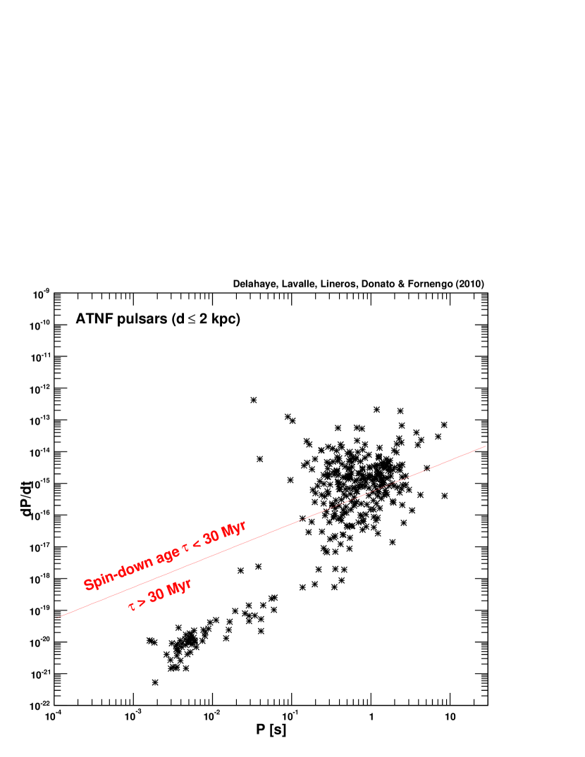
| J2000 | other name | distance | spin-down age | spin-down energy | Rank | known SNR |
| [kpc] | [kyr] | [ erg] | @ 5/100/1000 GeV | counterpart | ||
| J0633+1746 | Geminga | 0.16 | 342 | 1.25 | 1/2/4 | |
| J1932+1059 | B1929+10 | 0.36 | 3,100 | 11.9 | 2/-/- | |
| J1908+0734 | 0.58 | 4,080 | 17.9 | 3/-/- | ||
| J1741-2054 | 0.25 | 387 | 0.47 | 4/5/- | ||
| J0953+0755 | B0950+08 | 0.26 | 17,500 | 54.2 | 5/-/- | |
| J2043+2740 | 1.13 | 1,200 | 25.9 | -/1/- | ||
| J1057-5226 | B1055-52 | 0.72 | 535 | 2.8 | -/3/- | |
| J0659+1414 | B0656+14 | 0.29 | 111 | 0.18 | -/4/2 | Monogem |
| J0835-4510 | B0833-45 | 0.29 | 11.3 | 0.99 | -/-/1 | Vela |
| J1740+1000 | 1.24 | 114 | 1.1 | -/-/3 | ||
| J0742-2822 | B0740-28 | 1.89 | 157 | 1.23 | -/-/5 | |
| J1549-4848 | 1.54 | 324 | 0.8 | -/-/6 |
We selected local pulsars from the ATNF catalog, imposing a few constraints. First, we applied a radial cut-off of 2 kpc, as for the SNR treatment, farther pulsars being accounted for with a smooth spatial distribution modeling. For the latter, we adopted the L04 model, as for distant SNRs (see Sect. 4.4.1 for more details). Considering energies above the GeV scale imposes an upper limit of the pulsar age Myr, which decreases to 1 Myr above 100 GeV (see Fig. 7). We therefore restrict our sample by requiring that the ages Myr. This selection procedure is depicted in Fig. 13, where the local ATNF pulsars are reported in the - plane. Our final sample contains a bit more than 200 objects located at fewer than 2 kpc from the Earth, which is quite large compared to the number of observed SNRs, i.e. 27, discussed in Sect. 4.4.2.
The positron flux derived from this pulsar selection is obviously identical to the pulsar contribution to the electron flux discussed in Sect. 4.4.2, because of the pair production mechanism, and is shown in the right panel of Fig. 12. We remind the reader that a SNR counterpart was systematically added to each local pulsar, except for pulsars that already had an observed and identified SNR counterpart featuring in our SNR list. In case of a non-observed SNR counterpart, we assumed a radio flux to set its spectrum normalization (see Sect. 11). These non-observed SNR counterparts contribute only to the electron flux, which is reported in the middle panel of Fig. 12.
As briefly mentioned in Sect. 4.4.2, using the spin-down approximation to constrain the energy released in the form of electron-positron pairs leads pulsars to be important sources of local high energy electrons and positrons, as intense as the observed local SNRs. We employed a pair conversion efficiency of in this calculation, which might be optimistic, but still, decreasing this efficiency to a few percent would lead to a quite significant contribution to the local electron and positron budget. It is noteworthy that the local positron flux is dominated by a few objects among our 200 selected objects. The main sources and their properties are listed in Table 4. Although pulsar modeling is subject to many and large theoretical uncertainties, and despite the simplistic model we have employed to set the individual normalizations, our results suggest that SNRs might not be the only prominent sources of electron and positron cosmic rays. Nevertheless, this complete approach involving pulsars and SNRs in a self-consistent framework should be studied in greater detail, which may be promising for gaining deeper insights into the understanding of cosmic ray leptons.
A full template calculation of the positron flux including secondaries and primaries from distant and local pulsars is compared with existing data in the bottom left panel of Fig. 14. We used the data from HEAT (DuVernois et al. 2001), CAPRICE (Boezio et al. 2000), and AMS-01 (Alcaraz et al. 2000), which provide constraints at energies lower than 20 GeV only. From this plot, we see that secondaries can already account for a large fraction of the low energy positron flux, which constrains the properties of the additional primaries. We have in fact some freedom to tune the normalization and the spectral indices of the distant and local component, since they are poorly constrained. For the normalization, we have to adjust the pair conversion efficiency to values lower than 0.1, which reinforces the idea that pulsars can contribute to the local electron and positron flux quite naturally. This is discussed further when tackling the positron fraction case in Sect. 6.2. Likewise, there is no particular need to invoke hard spectral indices . The parameters that we have used are summarized in Table 5.
Finally, as for local contributions to the electron flux, we again point out that using the Thomson approximation to deal with the energy losses can lead to large errors and fake predictions of very peaky features in the overall positron spectrum.
6 Full electron and positron results — discussion
In this section, we now perform a template calculation with reasonable parameters for all previously discussed ingredients to demonstrate that pure astrophysical processes easily account for current measurements. It is quite simple to find configurations in good agreement with the data of the sum of electrons plus positrons or/and on the positron fraction, but it is far more difficult to find additional agreement with the separate electron and positron data. Many other studies have focused only on a few of these data sets, more rarely on all together.
As an important and preliminary remark, we emphasize that playing with the parameters associated with very few local sources within reasonable ranges allows us to fit all the data quite easily, though roughly, simply by adjusting the low/high energy source hierarchy. Nevertheless, for the sake of illustration, we attempt to use the full set of observational constraints that we dispose of without turning around. This is to illustrate how difficult and complex this self-consistent exercise can be. However, to simplify the discussion, we stick to the med set of propagation parameters, keeping in mind that uncertainties affecting propagation lead to order of magnitude uncertainty in the overall predictions. For the solar modulation, we use a Fisk potential of 600 MV.
In addition to our template calculation, the data themselves, when assumed trustworthy, can provide the actual separate positron and electron fluxes at the Earth. If we define and as the electron flux and the positron flux, respectively, and assume that some fitting functions and for the measured total flux (e.g. from Fermi data) and for the positron fraction (e.g. from PAMELA data), respectively, exist and are known, we then readily find
| (62) | |||||
| (63) |
Although we do not perform the exercise in the following, we point out that obtaining individual predictions in good agreement with and in the relevant energy range automatically ensures close agreement with the measured positron fraction and total electron plus positron flux. This might sound tautological, but is still a helpful method if one wishes to optimize her/his preferred CR model.
6.1 Electron and positron spectra: separate fluxes and sum
| L04 | local SNRs | local SNRs | L04 | local pulsars | |
| SNRs | (Green) | (ATNF) | pulsars | (ATNF) | |
| Spectral index | 2.4 | 2.4 | 2.0 | 2.0 | |
| [ erg/100 yr] | 21 | from | |||
| Converted fraction [%] | - | - | - | - | 0.6 |
| [TeV] | 2.0 | 2.0 | 2.0 | 1.5 | 1.5 |
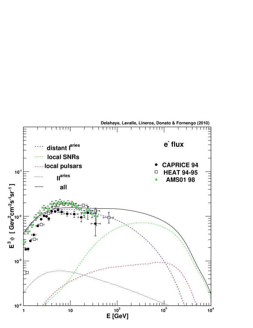
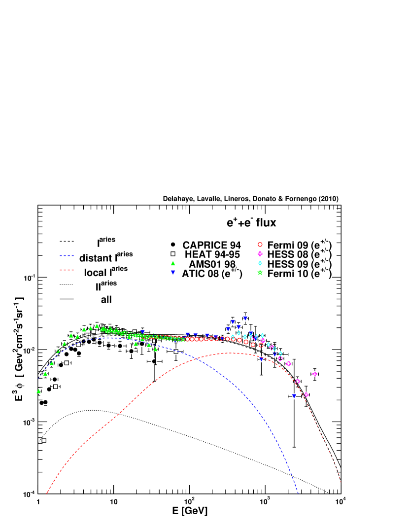
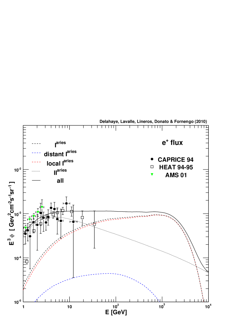
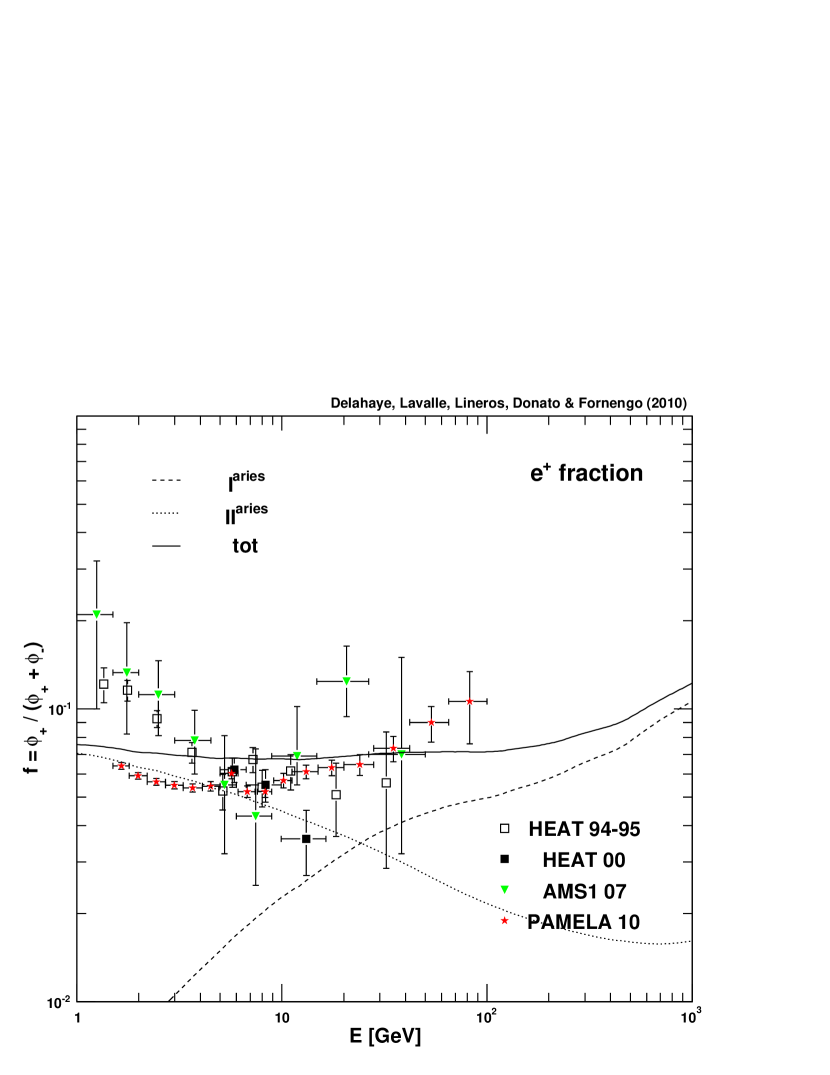
We compare a template calculation of the electron and positron fluxes with the available data. For electrons and positrons, as measured separately, we use the data from CAPRICE (Boezio et al. 2000), HEAT (DuVernois et al. 2001), and AMS-01 (Alcaraz et al. 2000). Note that these data are quite poorly constraining at high energy, since they refer to energies below a very few tens of GeV, and are affected by large statistical errors for the highest available energy bins. Future data from PAMELA and AMS-02 may certainly provide much tighter separate constraints on both components. For the sum of electrons and positrons, we employ the data from Fermi (Abdo et al. 2009b; Pesce-Rollins & for the Fermi-LAT Collaboration 2009), ATIC (Chang et al. 2008) and HESS (Aharonian et al. 2008, 2009a). It is meaningless to perform a fit, given the large theoretical uncertainties and the large number of parameters. We therefore empirically select the parameter sets that provide the smallest statistical errors whenever possible.
The top and bottom left panels of Fig. 14 show template results for the electron flux and the positron flux at the Earth, respectively. The parameters that we used to calculate all contributions are reported in Table 5.
For electrons, we see that the data of CAPRICE and AMS-01 are barely consistent, but we can identify a median configuration. Our template model is partly typified by a smooth SNR-plus-pulsar component (following the L04 spatial distribution) that fits the low energy part — the smooth pulsar contribution is actually completely negligible. We used a rather soft spectral index of 2.4 to shape this low energy smooth contribution, and a rather large value of (still consistent with theoretical or observational constraints — see Sect. 4.1). Nevertheless, we point out that using another spatial distribution, for instance with a stronger/softer spatial gradient, may have given the same result with other appropriate spectral indices and normalizations (see right panel of Fig. 5). This smooth component rapidly declines for energies higher than few tens GeV because of the 2 kpc radial cut-off around the Earth that we imposed before adding the local component. Above 10 GeV, we see that the local SNR contribution comes into play, clearly dominating over local pulsars. We underline that this hierarchy can hardly be considered as a generic prediction, since both types of sources are expected to provide similar amounts of electrons (see left and right panels of Fig. 12). Moreover, we adjusted the local SNR flux by a global factor of 6 with respect to our constraint recipe given in Eq. (50), which corresponds to using a mean magnetic field of G instead of 100. We remark that only a few sources dominate the overall flux (see Fig. 12 and Table 3), so modifying the parameters of these latter only may have a very strong impact on the predictions. We also note that another pulsar to SNR contribution ratio could easily lead to a similar overall shape for the electron flux. Likewise, slightly relaxing our chosen constraints either directly on the individual intensities or on the ages and distances, even across quite limited ranges, would allow far more freedom to shape each contribution differently. Nevertheless, the source hierarchy is here imposed by the observational constraints, which are relevant to Eq. (50) in the SNR case and Eq. (60) in the pulsar case; other methods based on different assumptions and different data would obviously provide different results. Finally, we stress that the local source flux is not characterized by individual prominent spiky peaks, as would be the case in the Thomson approximation for the energy losses (see Fig. 12). Additional constraints on sources of electrons come from the sum of electrons and positrons and from the positron fraction, as we later discuss.
For the positron flux, the important point is that secondaries are most likely predominant below 5 GeV. The corresponding calculation is less affected by theoretical uncertainties, so we could assume it to be a prediction. Indeed, the progenitor proton flux is not expected to vary significantly within a few kpc, and the main uncertainty apart from propagation is the average ISM gas density (Delahaye et al. 2009), such that the low energy positron flux may vary by at most a few tens of %. Beyond 5-10 GeV, there are poor constraints on the positron flux, so that the contribution of primaries may have any shape. The positron fraction provides additional information and constraints, as we later demonstrate. Nevertheless, we see that our choice of parameters for pulsars (distant and local) makes their contribution significant above GeV. From Table 5, it appears that assuming less than 1% of magnetic energy converted into electron-positron pairs is enough to make the pulsar contribution arise around 10 GeV; this is rather independent of the injected spectrum (we here assumed a spectral index of 2). We also remark that the smooth pulsar contribution is found to be negligible with respect to the local one. Finally, we emphasize that the overall spectral shape obtained for the positron flux weakly depends, in fact, on the assumed spectral index for pulsars. Indeed, as already shown in the right panel of Fig. 12, decreasing the intensity of a few old sources (such as Geminga or B1929+10) could easily result in a much harder spectrum at high energy and even a lower contribution below 10 GeV. Therefore, more tightly constraining the amplitude of the observed sources is a priority for future works.
The top right panel of Fig. 14 shows the sum of electrons and positrons, consistently with the separate results that we have just discussed above. The most distinctive information one can extract from this plot is probably the energy cut-off that explicitly appears around a few TeV, which obviously encourages us to set a cut-off energy around in this range. In our template calculation, the high energy part of the spectrum, above GeV, is actually dominated by our local SNR sample. This cannot be considered as a robust prediction, since we could have obtained a dominating pulsar contribution by slightly modifying the injection parameters. For instance, we could have reduced the local SNR yield, both depleted the supply from Geminga and increased that from Vela, and finally allowed a larger fraction of % of pair conversion.
We point out that the current constraints on sources are far too weak to ascertain the predictive power of our template calculation. Nevertheless, it is clear that the source modeling is the key point in the understanding of the high energy CR electrons, at least for identifying more clearly those few sources which may set most of the local flux. We also underline that it is important to challenge any CR electron prediction with the separate electron and positron data, since reproducing the sum does not necessarily ensure the relevance of the model. It will be important in the future to have independent sets of far higher quality data; PAMELA and AMS-02 carry many hopes.
6.2 Positron fraction
Measurements of the positron fraction contribute additional constraints that should be fulfilled consistently with the previous data. In the bottom right panel of Fig. 14, we have used the data from HEAT (Barwick et al. 1997; Beatty et al. 2004), AMS-01 (AMS-01 Collaboration et al. 2007), and PAMELA (PAMELA Collaboration et al. 2010). From this plot, our template calculation turns out to be consistent with the data, especially above 10 GeV. At lower energies, there are large discrepancies among the available measurements, which renders the interpretation complicated, though a more realistic treatment of the solar modulation — which is beyond the scope of this paper — might improve their level of consistency. Note that we can accommodate a slightly increasing positron fraction with very reasonable parameters for the local pulsar modeling, i.e. quite modest values of the converted energy fraction in pairs and spectral indices, without the need to tune the parameters for the sources individually. Indeed, for our local samples of SNRs and pulsars, we emphasize again that we constrained the whole contributions from observational constraints and fixed assumptions. It would have been quite easy to make this fraction increasing much rapidly with energy by considering additional assumptions for the pulsar power. We instead considered the simplest approach of the spin-down approximation for which the injection rate scales like the squared age (see Eq. 60). Had we adopted alternative modeling with a shallower dependence on the age (see e.g. Chi et al. 1996; Zhang & Cheng 2001; Profumo 2008), we would have placed more weight on younger objects, and thereby to the high energy part of the spectrum. As for the other measurements discussed above, we conclude that the positron fraction can be explained by pure astrophysical processes, even if the predictive power of our calculation remains weak.
6.2.1 Final comments
We wish here to highlight a few important points. First, we can fairly state that standard astrophysics is capable of reproducing the existing data, despite the large theoretical uncertainties associated with the flux calculation. Second, we attempted to convince the reader that an overall check of the separate electron and positron flux calculations against the associated separate data is mandatory to determine the relevance of a model: this step required the use of the four sets of data used in Fig. 14 separately. This was not covered in the literature so far, where most authors focused on either the sum of CR electrons and positrons or on the positron fraction. Third, we have shown that the full relativistic treatment of the energy losses could lead to a global spectral shape devoid of peaky structures. Fourth, we have discussed a template example where we fixed the local source hierarchy based on a few assumptions and observational constraints. It is clear, however, that a more refined analysis with a far more accurate source modeling will help us to reduce the theoretical uncertainties and clarify the local source hierarchy; it will also probably lead to different results. Nevertheless, we have proposed an exhaustive set of analytical tools together with a robust method to tackle such a detailed analysis. Finally, we stress that we have derived our template calculation using our med set of propagation parameters to facilitate the reading of the plots, and have therefore not discussed the uncertainties originating in the propagation side, which are actually large, as discussed in Sect. 4.3 for individual sources — see bottom right panel of Fig. 7, and Fig. 11.
7 Summary and conclusions
We attempted to perform an exhaustive study of the main ingredients relevant to the calculation of the high energy CR electron and positron fluxes in the GeV-TeV energy range. We have underlined the complexity of the source description, by emphasizing the potentially strong effects of nearby sources, and shown that though we can hardly predict the local electron and positron fluxes with accuracy, reasonable parameterizations of the source and the propagation modeling can fairly well and simultaneously account for the current measurements of (i) electrons, (ii) positrons, (iii) the sum of them, and (iv) the positron fraction. We summarize hereafter the way in which we have proceeded.
In Sect. 2, we presented our propagation modeling in detail. We reviewed the analytical solutions to the transport equation in Sects. 2.1 and 2.2 and derived explicit links between the source spectrum and the propagated spectrum in Sect. 2.3. More importantly, we developed in Sect. 2.4 a method to account for the relativistic energy losses, providing useful fit formulae that can be used for any inverse Compton processes involving a black-body photon target. We have indeed shown that the Thomson approximation was by far insufficient and could lead to fake predictions of peaky signatures in the electron spectrum as potential imprints of local sources. In Sect. 2.5, we recalled our propagation parameters with emphasis on the energy losses. In particular, we developed a quite tightly constrained local ISRF modeling and explained in detail how its different components result in decreasing steps in the overall energy loss function, as a consequence of Klein-Nishina effects.
In Sect. 3, we revisited the predictions for the secondary electron and positron fluxes, finding slight differences from the previous analysis we performed in Delahaye et al. (2009) — for positrons only, and using the Thomson approximation for the energy losses. These differences are caused by our novel relativistic treatment of the energy losses. We found a slightly harder secondary spectrum, with an overall flux higher by % at 100 GeV up to % at 1 TeV. We emphasized, however, that this can still not explain an increasing positron fraction. We provided fitting formulae of our results in Appendix B, valid in the med propagation setup.
In Sect. 4, we described in detail the calculation of the primary electron flux. We explored thoroughly the possible ways of normalizing the injection rate of CR electrons in Sect. 4.1, focusing on a smooth distribution of sources as well as on discrete sources, and showed that the theoretical uncertainties are impressively large, reaching 2 or 3 orders of magnitude. In particular, the fraction of energy transmitted to CR electrons is quite an issue. Nevertheless, we sketched a method to normalize an event-like source injection density from its measured radio flux, which allows us to use observational constraints whenever available. We demonstrated in Sect. 4.2 that any smooth spatial distribution of sources could be approximated with a mere -exponential disk up to very high accuracy for electrons of energy above a few tens of GeV, showing that the specific spatial distribution had negligible impact on the predictions, for which only the local density of sources really accounts. Since local effects are more important above a few tens of GeV, we exhaustively studied in Sect. 4.3 the impacts of the parameters relevant to the local event-like source description, i.e. the age, the distance and the spectral index, as well as of the propagation parameters (see Fig. 7). We notably illustrated how irrelevant the individual spectral indices were to inferring the overall spectral shape produced by a population of non-identical objects. We have shown that the overall spectrum was mostly set by a hardly predictable hierarchy in the local sources. The energy range characterizing a single contribution is mostly bounded from above by the age and cut-off energy, and from below by the distance. For the former bound, we demonstrated that the Thomson approximation led to erroneous predictions, with significant underestimates of the maximal energy and fake peaky features. We also demonstrated that changing the diffusion coefficient had a strong impact on the results. Finally, in Sect. 4.4, we discussed a template calculation including the constrained contributions of all known local sources lying within a distance of 2 kpc from the Earth, showing that pulsars might contribute as many primary electrons as SNRs. We again emphasized the quite poor predictive power that can be achieved even when accounting for observational constraints. This is mostly due to the theoretical uncertainties affecting the source modeling. Nevertheless, we indicated a few objects that probably dominate the overall high energy flux.
In Sect. 5, we studied the contribution of pulsars to the primary positron flux, using the spin-down approximation to constrain the injection rate of local pulsars. As for primary electrons, we demonstrated that the very large theoretical uncertainties makes it difficult to claim robust predictions.
For the local sources, we proposed a novel approach including not only known SNRs or pulsars, but also adding a SNR counterpart to each non-associated pulsar. Indeed, since a pulsar is the relic neutron star of a core-collapse supernova explosion, it should be accompanied by a SNR for consistency reasons. We accounted for these non-observed SNRs needing to have a radio flux below the current experimental sensitivities when normalizing their injection rates of electrons. In contrast, all SNRs are not expected to have a pulsar companion, in particular those SNRs coming from SN1a explosions. A more refined and realistic modeling of sources including such composite contributions and further accounting for the dynamics of CR injection remains to be considered in terms of electron flux. This is, however, far beyond the scope of this paper, though we attempted to pave the road for such an ambitious study.
Finally, in Sect. 6, we presented a template calculation including all sources of primaries, in which we used observational constraints whenever available (see Fig. 14). We considered the true complexity of the source description within a self-consistent framework, at variance with many other studies that merely added local contributions to other so-called standard predictions. We demonstrated that for reasonable assumptions about the parameters of both the local and distant components, all of the discussed astrophysical processes can account rather well for all measurements of cosmic ray electrons and positrons independently. We pointed out that comparing any prediction with only the positron fraction or the sum of electrons and positrons is incomplete, and does not ensure its consistency. We emphasize that our template calculation cannot stand for a robust prediction because of the very large theoretical uncertainties underlined along this paper. Our results should instead be considered as a proof that current measurements are compatible with pure astrophysical processes, so that one can hardly claim any prominent anomaly at the moment. More importantly, we hope to have shown that a standard model of CR electrons, standard in the sense that departures from observational data would sign something unexpected or exotic, is far from being reached, since we even do not control the modeling of the local environment (mostly the sources), which is of paramount importance here. This may have drastic consequences; for instance, it indicates how well one can control or predict the CR electron contribution to the high energy part of the Galactic diffuse gamma-ray emission, or to the diffuse radio emission. In turn, however, this diffuse emission can provide additional information and constraints on the astrophysical processes at stake. More accurate predictions may only emerge for observables that involve features averaged over large spatial and/or timescales, to guarantee protection against potentially large and hardly controllable fluctuations in the calculation results. This is for instance the case for high energy stable nuclei.
Such conclusions may sound disappointing but they imply many interesting by-products and open anyway a very broad landscape for future theoretical improvements. For instance, we have shown that a few local sources may dominate the electron flux. If so, far more refined models of these sources may allow us to use electrons as independent tracers of the local diffusion coefficient. Positive measurements of anisotropies in the CR electron flux might also provide insights in the power hierarchy among local sources, provided this hierarchy is strong; indeed, each flux energy-bin is most likely filled by contributions from several sources located at different positions in the sky. In any case, the connection between the local CR electrons and the physics of sources is probably one of the most important issue to investigate further in future studies; low energy protons might also provide additional constraints on the local sources.
Finally, for the searches for exotic signatures, e.g. from dark matter annihilation or decay, the large theoretical uncertainties associated with the astrophysical processes prevent us from deriving much stronger constraints at the moment, unfortunately. Nevertheless, we underline that invoking any exotic contribution is absolutely unnecessary to understand the current data, and is thereby quite easily arguable. It seems therefore likely that models which are over-tuned to fit the positron data, aside from independent motivations coming from particle physics, are of very weak relevance. We recall that almost all well-studied dark matter particle candidates, e.g. in the framework of supersymmetric or extra-dimensional theories, are expected to manifest themselves in neither the local positron nor antiproton spectra (e.g. Lavalle et al. 2008a; Delahaye et al. 2008; Donato et al. 2004). Were dark matter annihilation really to enhance the positron budget, far more work would be necessary to prove it, by means of multi-messenger and multiwavelength approaches. This would require great efforts to face the complexity of the astrophysical backgrounds and, more importantly, this will have to rely on self-consistent calculations of both the signals and backgrounds.
Acknowledgements.
We are deeply indebted to P. Salati for very inspiring comments and previous collaborations on related topics. We would like to thank A. Fiasson and Y. Gallant for very helpful discussions about SNRs and pulsars. We are also grateful to the participants of the two Workshops on Diffuse -ray emission, organized in 2008 and 2009 in the frame of the French GDR PCHE, for fruitful debates related to the topic666A short summary of the workshops and the website addresses are available in Lavalle et al. (2009).. TD thanks the International Doctorate on Astro-Particle Physics (IDAPP) and the Rhône-Alpes region (Explora’Doc program) for financial support. JL is grateful to LAPTH for hospitality during parts of this study. NF acknowledges support of the Spanish MICINN’s Consolider–Ingenio 2010 Programme under grant MULTIDARK CSD2009-00064. This work was partly supported by research grants funded jointly by Ministero dell’Istruzione, dell’Università e della Ricerca (MIUR), by the University of Torino (UniTO), by the Istituto Nazionale di Fisica Nucleare (INFN) within the Astroparticle Physics Project, by the Italian Space Agency (ASI) under contract N∘ I/088/06/0 and by the French Programme National de Cosmologie (PNC).References
- Abdo et al. (2009a) Abdo, A. A., Ackermann, M., Ajello, M., et al. 2009a, Science, 325, 840
- Abdo et al. (2009b) Abdo, A. A., Ackermann, M., Ajello, M., et al. 2009b, Physical Review Letters, 102, 181101
- Abdo et al. (2008) Abdo, A. A., Ackermann, M., Atwood, W. B., et al. 2008, Science, 322, 1218
- Aharonian et al. (2009a) Aharonian, F., Akhperjanian, A. G., Anton, G., et al. 2009a, A&A, 508, 561
- Aharonian et al. (2008) Aharonian, F., Akhperjanian, A. G., Barres de Almeida, U., et al. 2008, Physical Review Letters, 101, 261104
- Aharonian et al. (2009b) Aharonian, F., Akhperjanian, A. G., de Almeida, U. B., et al. 2009b, ApJ, 692, 1500
- Aharonian et al. (1995) Aharonian, F. A., Atoyan, A. M., & Voelk, H. J. 1995, A&A, 294, L41
- Ahlers et al. (2009) Ahlers, M., Mertsch, P., & Sarkar, S. 2009, Phys. Rev. D, 80, 123017
- Alcaraz et al. (2000) Alcaraz, J., Alpat, B., Ambrosi, G., et al. 2000, Physics Letters B, 484, 10
- Alvarez et al. (2001) Alvarez, H., Aparici, J., May, J., & Reich, P. 2001, A&A, 372, 636
- AMS-01 Collaboration et al. (2007) AMS-01 Collaboration, Aguilar, M., Alcaraz, J., et al. 2007, Physics Letters B, 646, 145
- Anderson et al. (1996) Anderson, S. B., Cadwell, B. J., Jacoby, B. A., et al. 1996, ApJ, 468, L55+
- Asano et al. (2007) Asano, M., Matsumoto, S., Okada, N., & Okada, Y. 2007, Phys. Rev. D, 75, 063506
- Atoyan & Aharonian (1996) Atoyan, A. M. & Aharonian, F. A. 1996, MNRAS, 278, 525
- Atoyan et al. (1995) Atoyan, A. M., Aharonian, F. A., & Völk, H. J. 1995, Phys. Rev. D, 52, 3265
- Baltz & Edsjö (1998) Baltz, E. A. & Edsjö, J. 1998, Phys. Rev. D, 59, 023511
- Baltz & Wai (2004) Baltz, E. A. & Wai, L. 2004, Phys. Rev. D, 70, 023512
- Barwick et al. (1997) Barwick, S. W., Beatty, J. J., Bhattacharyya, A., et al. 1997, ApJ, 482, L191+
- Battiston (2007) Battiston, R. 2007, Nuclear Physics B Proceedings Supplements, 166, 19
- Beatty et al. (2004) Beatty, J. J., Bhattacharyya, A., Bower, C., et al. 2004, Physical Review Letters, 93, 241102
- Berezhko et al. (2003) Berezhko, E. G., Ksenofontov, L. T., Ptuskin, V. S., Zirakashvili, V. N., & Völk, H. J. 2003, A&A, 410, 189
- Berezinskii et al. (1990) Berezinskii, V. S., Bulanov, S. V., Dogiel, V. A., & Ptuskin, V. S. 1990, Astrophysics of cosmic rays (Amsterdam: North-Holland, 1990, edited by Ginzburg, V.L.)
- Bergström et al. (2008) Bergström, L., Bringmann, T., & Edsjö, J. 2008, Phys. Rev. D, 78, 103520
- Blair et al. (2005) Blair, W. P., Sankrit, R., & Raymond, J. C. 2005, AJ, 129, 2268
- Blair et al. (2009) Blair, W. P., Sankrit, R., Torres, S. I., Chayer, P., & Danforth, C. W. 2009, ApJ, 692, 335
- Blandford & Eichler (1987) Blandford, R. & Eichler, D. 1987, Phys. Rep, 154, 1
- Blasi (2009) Blasi, P. 2009, Physical Review Letters, 103, 051104
- Blasi & Serpico (2009) Blasi, P. & Serpico, P. D. 2009, Physical Review Letters, 103, 081103
- Blondin et al. (2001) Blondin, J. M., Chevalier, R. A., & Frierson, D. M. 2001, ApJ, 563, 806
- Blumenthal & Gould (1970) Blumenthal, G. R. & Gould, R. J. 1970, Reviews of Modern Physics, 42, 237
- Boezio et al. (2000) Boezio, M., Carlson, P., Francke, T., et al. 2000, ApJ, 532, 653
- Bonatto & Bica (2009) Bonatto, C. & Bica, E. 2009, MNRAS, 278
- Borka Jovanović & Urošević (2009) Borka Jovanović, V. & Urošević, D. 2009, ArXiv e-prints 0904.2261
- Boulares (1989) Boulares, A. 1989, ApJ, 342, 807
- Brisken et al. (2003) Brisken, W. F., Thorsett, S. E., Golden, A., & Goss, W. M. 2003, ApJ, 593, L89
- Brogan et al. (2006) Brogan, C. L., Gelfand, J. D., Gaensler, B. M., Kassim, N. E., & Lazio, T. J. W. 2006, ApJ, 639, L25
- Bucciantini (2008) Bucciantini, N. 2008, Advances in Space Research, 41, 491
- Bulanov & Dogel (1974) Bulanov, S. V. & Dogel, V. A. 1974, Ap&SS, 29, 305
- Burrows (2000) Burrows, A. 2000, Nature, 403, 727
- Bykov et al. (2004) Bykov, A. M., Krassilchtchikov, A. M., Uvarov, Y. A., et al. 2004, A&A, 427, L21
- Byun et al. (2006) Byun, D.-Y., Koo, B.-C., Tatematsu, K., & Sunada, K. 2006, ApJ, 637, 283
- Caprioli et al. (2009) Caprioli, D., Blasi, P., & Amato, E. 2009, MNRAS, 396, 2065
- Caraveo et al. (2001) Caraveo, P. A., De Luca, A., Mignani, R. P., & Bignami, G. F. 2001, ApJ, 561, 930
- Case & Bhattacharya (1998) Case, G. L. & Bhattacharya, D. 1998, ApJ, 504, 761
- Castelletti & Dubner (2005) Castelletti, G. & Dubner, G. 2005, A&A, 440, 171
- Castelletti et al. (2003) Castelletti, G., Dubner, G., Golap, K., et al. 2003, AJ, 126, 2114
- Catena et al. (2009) Catena, R., Fornengo, N., Pato, M., Pieri, L., & Masiero, A. 2009, ArXiv e-prints
- Cha et al. (1999) Cha, A. N., Sembach, K. R., & Danks, A. C. 1999, ApJ, 515, L25
- Chang et al. (2008) Chang, J., Adams, J. H., Ahn, H. S., et al. 2008, Nature, 456, 362
- Cheng et al. (1976) Cheng, A., Ruderman, M., & Sutherland, P. 1976, ApJ, 203, 209
- Cheng et al. (1986) Cheng, K. S., Ho, C., & Ruderman, M. 1986, ApJ, 300, 500
- Chi et al. (1996) Chi, X., Cheng, K. S., & Young, E. C. M. 1996, ApJ, 459, L83+
- Cirelli et al. (2008) Cirelli, M., Franceschini, R., & Strumia, A. 2008, Nuclear Physics B, 800, 204
- Cowsik & Lee (1979) Cowsik, R. & Lee, M. A. 1979, ApJ, 228, 297
- Delahaye et al. (2009) Delahaye, T., Donato, F., Fornengo, N., et al. 2009, A&A, 501, 821
- Delahaye et al. (2008) Delahaye, T., Lineros, R., Donato, F., Fornengo, N., & Salati, P. 2008, Phys. Rev. D, 77, 063527
- Diehl et al. (2006) Diehl, R., Halloin, H., Kretschmer, K., et al. 2006, Nature, 439, 45
- Donato et al. (2004) Donato, F., Fornengo, N., Maurin, D., Salati, P., & Taillet, R. 2004, Phys. Rev. D, 69, 063501
- Donato et al. (2009) Donato, F., Maurin, D., Brun, P., Delahaye, T., & Salati, P. 2009, Physical Review Letters, 102, 071301
- Donato et al. (2002) Donato, F., Maurin, D., & Taillet, R. 2002, Astronomy and Astrophys., 381, 539
- Duncan et al. (1997) Duncan, A. R., Stewart, R. T., Haynes, R. F., & Jones, K. L. 1997, MNRAS, 287, 722
- DuVernois et al. (2001) DuVernois, M. A., Barwick, S. W., Beatty, J. J., et al. 2001, ApJ, 559, 296
- Ellison & Cassam-Chenaï (2005) Ellison, D. C. & Cassam-Chenaï, G. 2005, ApJ, 632, 920
- Ellison et al. (2007) Ellison, D. C., Patnaude, D. J., Slane, P., Blasi, P., & Gabici, S. 2007, ApJ, 661, 879
- Erber (1966) Erber, T. 1966, Reviews of Modern Physics, 38, 626
- Ferrière (2001) Ferrière, K. M. 2001, Reviews of Modern Physics, 73, 1031
- Fiasson et al. (2008) Fiasson, A., Hinton, J. A., Gallant, Y., & et al. 2008, in International Cosmic Ray Conference, Vol. 2, 719–722
- Fisk (1971) Fisk, L. A. 1971, J. Geophys. Res., 76, 221
- Fixsen (2009) Fixsen, D. J. 2009, ArXiv e-prints
- Fuerst et al. (1997) Fuerst, E., Reich, W., & Aschenbach, B. 1997, A&A, 319, 655
- Furst et al. (1989) Furst, E., Hummel, E., Reich, W., et al. 1989, A&A, 209, 361
- Gaensler & Frail (2000) Gaensler, B. M. & Frail, D. A. 2000, Nature, 406, 158
- Gaensler & Slane (2006) Gaensler, B. M. & Slane, P. O. 2006, ARA&A, 44, 17
- Gamezo et al. (2003) Gamezo, V. N., Khokhlov, A. M., Oran, E. S., Chtchelkanova, A. Y., & Rosenberg, R. O. 2003, Science, 299, 77
- Gerardy & Fesen (2007) Gerardy, C. L. & Fesen, R. A. 2007, MNRAS, 376, 929
- Ginzburg & Syrovatskii (1964) Ginzburg, V. L. & Syrovatskii, S. I. 1964, The Origin of Cosmic Rays (The Origin of Cosmic Rays, New York: Macmillan, 1964)
- Ginzburg & Syrovatskii (1965) Ginzburg, V. L. & Syrovatskii, S. I. 1965, ARA&A, 3, 297
- Gorham et al. (1996) Gorham, P. W., Ray, P. S., Anderson, S. B., Kulkarni, S. R., & Prince, T. A. 1996, ApJ, 458, 257
- Graham et al. (1982) Graham, D. A., Haslam, C. G. T., Salter, C. J., & Wilson, W. E. 1982, A&A, 109, 145
- Green (2005) Green, D. A. 2005, Memorie della Societa Astronomica Italiana, 76, 534
- Green (2009) Green, D. A. 2009, Bull. Astron. Soc. Ind., 37, 45
- Harding et al. (2008) Harding, A. K., Stern, J. V., Dyks, J., & Frackowiak, M. 2008, ApJ, 680, 1378
- Harrus et al. (2004) Harrus, I. M., Slane, P. O., Hughes, J. P., & Plucinsky, P. P. 2004, ApJ, 603, 152
- Hooper et al. (2009) Hooper, D., Blasi, P., & Dario Serpico, P. 2009, Journal of Cosmology and Astro-Particle Physics, 1, 25
- Hooper & Kribs (2004) Hooper, D. & Kribs, G. D. 2004, Phys. Rev. D, 70, 115004
- Humphreys (1978) Humphreys, R. M. 1978, ApJS, 38, 309
- Jaffe et al. (2010) Jaffe, T. R., Leahy, J. P., Banday, A. J., et al. 2010, MNRAS, 401, 1013
- Janka et al. (2007) Janka, H., Langanke, K., Marek, A., Martínez-Pinedo, G., & Müller, B. 2007, Phys. Rep, 442, 38
- Jansson et al. (2009) Jansson, R., Farrar, G. R., Waelkens, A. H., & Enßlin, T. A. 2009, Journal of Cosmology and Astro-Particle Physics, 7, 21
- Jones (1965) Jones, F. C. 1965, Physical Review, 137, 1306
- Kamae et al. (2006) Kamae, T., Karlsson, N., Mizuno, T., Abe, T., & Koi, T. 2006, ApJ, 647, 692
- Kaplan et al. (2008) Kaplan, D. L., Chatterjee, S., Gaensler, B. M., & Anderson, J. 2008, ApJ, 677, 1201
- Kaplan et al. (2004) Kaplan, D. L., Frail, D. A., Gaensler, B. M., et al. 2004, ApJS, 153, 269
- Kaplan et al. (2006) Kaplan, D. L., Gaensler, B. M., Kulkarni, S. R., & Slane, P. O. 2006, ApJS, 163, 344
- Katsuda et al. (2009) Katsuda, S., Petre, R., Hwang, U., et al. 2009, PASJ, 61, 155
- Katsuda et al. (2008) Katsuda, S., Tsunemi, H., & Mori, K. 2008, ApJ, 678, L35
- Kobayashi et al. (2004) Kobayashi, T., Komori, Y., Yoshida, K., & Nishimura, J. 2004, ApJ, 601, 340
- Kothes et al. (2006) Kothes, R., Fedotov, K., Foster, T. J., & Uyanıker, B. 2006, A&A, 457, 1081
- Kothes et al. (2008) Kothes, R., Landecker, T. L., Reich, W., Safi-Harb, S., & Arzoumanian, Z. 2008, ApJ, 687, 516
- Ladouceur & Pineault (2008) Ladouceur, Y. & Pineault, S. 2008, A&A, 490, 197
- Lavalle et al. (2009) Lavalle, J., Marcowith, A., & Maurin, D. 2009, in Proc. SF2A-2009, ed. M. Heydari-Malayeri, C. Reyl’E, & R. Samadi, 165–+
- Lavalle et al. (2008a) Lavalle, J., Nezri, E., Athanassoula, E., Ling, F.-S., & Teyssier, R. 2008a, Phys. Rev. D, 78, 103526
- Lavalle et al. (2007) Lavalle, J., Pochon, J., Salati, P., & Taillet, R. 2007, A&A, 462, 827
- Lavalle et al. (2008b) Lavalle, J., Yuan, Q., Maurin, D., & Bi, X.-J. 2008b, A&A, 479, 427
- Lazendic & Slane (2006) Lazendic, J. S. & Slane, P. O. 2006, ApJ, 647, 350
- Leahy & Tian (2006) Leahy, D. & Tian, W. 2006, A&A, 451, 251
- Leahy et al. (1986) Leahy, D. A., Naranan, S., & Singh, K. P. 1986, MNRAS, 220, 501
- Leahy et al. (1991) Leahy, D. A., Nousek, J., & Hamilton, A. J. S. 1991, ApJ, 374, 218
- Leahy & Tian (2007) Leahy, D. A. & Tian, W. W. 2007, A&A, 461, 1013
- Longair (1994) Longair, M. S. 1994, High energy astrophysics. Vol.2: Stars, the galaxy and the interstellar medium (Cambridge: Cambridge University Press, —c1994, 2nd ed.)
- Lorimer (2004) Lorimer, D. R. 2004, in IAU Symposium, Vol. 218, Young Neutron Stars and Their Environments, ed. F. Camilo & B. M. Gaensler, 105–+
- Lucek & Bell (2000) Lucek, S. G. & Bell, A. R. 2000, MNRAS, 314, 65
- Madau et al. (1998) Madau, P., della Valle, M., & Panagia, N. 1998, MNRAS, 297, L17+
- Malkov & O’C Drury (2001) Malkov, M. A. & O’C Drury, L. 2001, Reports on Progress in Physics, 64, 429
- Malyshev et al. (2009) Malyshev, D., Cholis, I., & Gelfand, J. 2009, Phys. Rev. D, 80, 063005
- Manchester et al. (2005) Manchester, R. N., Hobbs, G. B., Teoh, A., & Hobbs, M. 2005, AJ, 129, 1993
- Mantovani et al. (1982) Mantovani, F., Nanni, M., Salter, C. J., & Tomasi, P. 1982, A&A, 105, 176
- Maurin et al. (2001) Maurin, D., Donato, F., Taillet, R., & Salati, P. 2001, ApJ, 555, 585
- Mavromatakis (2003) Mavromatakis, F. 2003, A&A, 408, 237
- Mavromatakis et al. (2004) Mavromatakis, F., Aschenbach, B., Boumis, P., & Papamastorakis, J. 2004, A&A, 415, 1051
- Mavromatakis et al. (2002) Mavromatakis, F., Boumis, P., Papamastorakis, J., & Ventura, J. 2002, A&A, 388, 355
- Mazzali et al. (2007) Mazzali, P. A., Röpke, F. K., Benetti, S., & Hillebrandt, W. 2007, Science, 315, 825
- McCullough et al. (2002) McCullough, P. R., Fields, B. D., & Pavlidou, V. 2002, ApJ, 576, L41
- Mertsch & Sarkar (2009) Mertsch, P. & Sarkar, S. 2009, Physical Review Letters, 103, 081104
- Miceli et al. (2008) Miceli, M., Bocchino, F., & Reale, F. 2008, ApJ, 676, 1064
- Morlino et al. (2009) Morlino, G., Amato, E., & Blasi, P. 2009, MNRAS, 392, 240
- Moskalenko & Strong (1998) Moskalenko, I. V. & Strong, A. W. 1998, ApJ, 493, 694
- Mufson et al. (1986) Mufson, S. L., McCollough, M. L., Dickel, J. R., et al. 1986, AJ, 92, 1349
- Neufeld et al. (2007) Neufeld, D. A., Hollenbach, D. J., Kaufman, M. J., et al. 2007, ApJ, 664, 890
- Nomoto et al. (1984) Nomoto, K., Thielemann, F., & Yokoi, K. 1984, ApJ, 286, 644
- Norbury & Townsend (2007) Norbury, J. W. & Townsend, L. W. 2007, Nuclear Instruments and Methods in Physics Research B, 254, 187
- Odegard (1986) Odegard, N. 1986, ApJ, 301, 813
- Ostriker & Gunn (1969) Ostriker, J. P. & Gunn, J. E. 1969, ApJ, 157, 1395
- Paczynski (1990) Paczynski, B. 1990, ApJ, 348, 485
- PAMELA Collaboration et al. (2010) PAMELA Collaboration, Adriani, O., Barbarino, G. C., et al. 2010, Astroparticle Physics, 34, 1
- PAMELA Collaboration et al. (2009) PAMELA Collaboration, Adriani, O., Barbarino, G. C., et al. 2009, Nature, 458, 607
- Pannuti & Allen (2004) Pannuti, T. G. & Allen, G. E. 2004, Advances in Space Research, 33, 434
- Pesce-Rollins & for the Fermi-LAT Collaboration (2009) Pesce-Rollins, M. & for the Fermi-LAT Collaboration. 2009, ArXiv e-prints
- Pfeffermann et al. (1991) Pfeffermann, E., Aschenbach, B., & Predehl, P. 1991, A&A, 246, L28
- Pieri et al. (2009) Pieri, L., Lavalle, J., Bertone, G., & Branchini, E. 2009, ArXiv e-prints
- Pineault et al. (1993) Pineault, S., Landecker, T. L., Madore, B., & Gaumont-Guay, S. 1993, AJ, 105, 1060
- Pineault et al. (1997) Pineault, S., Landecker, T. L., Swerdlyk, C. M., & Reich, W. 1997, A&A, 324, 1152
- Plucinsky et al. (1996) Plucinsky, P. P., Snowden, S. L., Aschenbach, B., et al. 1996, ApJ, 463, 224
- Porter et al. (2008) Porter, T. A., Moskalenko, I. V., Strong, A. W., Orlando, E., & Bouchet, L. 2008, ApJ, 682, 400
- Profumo (2008) Profumo, S. 2008, ArXiv e-prints
- Putze et al. (2010) Putze, A., Derome, L., & Maurin, D. 2010, A&A, 516, A66+
- Redman & Meaburn (2005) Redman, M. P. & Meaburn, J. 2005, MNRAS, 356, 969
- Reich et al. (1992) Reich, W., Fuerst, E., & Arnal, E. M. 1992, A&A, 256, 214
- Reich et al. (2003) Reich, W., Zhang, X., & Fürst, E. 2003, A&A, 408, 961
- Rosado & Gonzalez (1981) Rosado, M. & Gonzalez, J. 1981, Revista Mexicana de Astronomia y Astrofisica, 5, 93
- Ruderman & Sutherland (1975) Ruderman, M. A. & Sutherland, P. G. 1975, ApJ, 196, 51
- Salati (2003) Salati, P. 2003, Physics Letters B, 571, 121
- Schlickeiser & Ruppel (2009) Schlickeiser, R. & Ruppel, J. 2009, ArXiv e-prints
- Shaviv et al. (2009) Shaviv, N. J., Nakar, E., & Piran, T. 2009, Physical Review Letters, 103, 111302
- Shen (1970) Shen, C. S. 1970, ApJ, 162, L181+
- Shikaze et al. (2007) Shikaze, Y., Haino, S., Abe, K., et al. 2007, Astroparticle Physics, 28, 154
- Shinn et al. (2006) Shinn, J., Min, K. W., Lee, C., et al. 2006, ApJ, 644, L189
- Shinn et al. (2007) Shinn, J.-H., Min, K. W., Sankrit, R., et al. 2007, ApJ, 670, 1132
- Silk & Srednicki (1984) Silk, J. & Srednicki, M. 1984, Physical Review Letters, 53, 624
- Sofue et al. (1980) Sofue, Y., Furst, E., & Hirth, W. 1980, PASJ, 32, 1
- Strom & Stappers (2000) Strom, R. G. & Stappers, B. W. 2000, in Astronomical Society of the Pacific Conference Series, Vol. 202, IAU Colloq. 177: Pulsar Astronomy - 2000 and Beyond, ed. M. Kramer, N. Wex, & R. Wielebinski, 509–+
- Strong & Moskalenko (1998) Strong, A. W. & Moskalenko, I. V. 1998, ApJ, 509, 212
- Strong et al. (2007) Strong, A. W., Moskalenko, I. V., & Ptuskin, V. S. 2007, Annual Review of Nuclear and Particle Science, 57, 285
- Strong et al. (2000) Strong, A. W., Moskalenko, I. V., & Reimer, O. 2000, ApJ, 537, 763
- Stupar et al. (2007) Stupar, M., Parker, Q. A., & Filipović, M. D. 2007, MNRAS, 374, 1441
- Sturrock (1970) Sturrock, P. A. 1970, Nature, 227, 465
- Sturrock (1971) Sturrock, P. A. 1971, ApJ, 164, 529
- Sun et al. (2006) Sun, X. H., Reich, W., Han, J. L., Reich, P., & Wielebinski, R. 2006, A&A, 447, 937
- Tan & Ng (1983) Tan, L. C. & Ng, L. K. 1983, Journal of Physics G Nuclear Physics, 9, 1289
- Tatischeff (2009) Tatischeff, V. 2009, A&A, 499, 191
- Taylor et al. (2003) Taylor, A. R., Gibson, S. J., Peracaula, M., et al. 2003, AJ, 125, 3145
- Taylor et al. (1993) Taylor, J. H., Manchester, R. N., & Lyne, A. G. 1993, ApJS, 88, 529
- Troja et al. (2008) Troja, E., Bocchino, F., Miceli, M., & Reale, F. 2008, A&A, 485, 777
- Uyaniker et al. (2002) Uyaniker, B., Kothes, R., & Brunt, C. M. 2002, ApJ, 565, 1022
- Valinia & Marshall (1998) Valinia, A. & Marshall, F. E. 1998, ApJ, 505, 134
- van den Bergh & Tammann (1991) van den Bergh, S. & Tammann, G. A. 1991, ARA&A, 29, 363
- Vinyaikin (2007) Vinyaikin, E. N. 2007, Astronomy Reports, 51, 570
- Welsh & Sallmen (2003) Welsh, B. Y. & Sallmen, S. 2003, A&A, 408, 545
- Welsh et al. (2001) Welsh, B. Y., Sfeir, D. M., Sallmen, S., & Lallement, R. 2001, A&A, 372, 516
- Woosley & Janka (2005) Woosley, S. & Janka, T. 2005, Nature Physics, 1, 147
- Xiao et al. (2008) Xiao, L., Fürst, E., Reich, W., & Han, J. L. 2008, A&A, 482, 783
- Xiao et al. (2009) Xiao, L., Reich, W., Fürst, E., & Han, J. L. 2009, ArXiv e-prints
- Yar-Uyaniker et al. (2004) Yar-Uyaniker, A., Uyaniker, B., & Kothes, R. 2004, ApJ, 616, 247
- Yüksel et al. (2009) Yüksel, H., Kistler, M. D., & Stanev, T. 2009, Physical Review Letters, 103, 051101
- Yusifov & Küçük (2004) Yusifov, I. & Küçük, I. 2004, A&A, 422, 545
- Zeiger et al. (2008) Zeiger, B. R., Brisken, W. F., Chatterjee, S., & Goss, W. M. 2008, ApJ, 674, 271
- Zhang & Cheng (2001) Zhang, L. & Cheng, K. S. 2001, A&A, 368, 1063
Appendix A Analytical solutions of the spatial integral
We briefly present the solutions of the spatial integral of the Green function convolved with a disk–like spatial distribution for sources. We distinguish two cases: (i) a homogeneous flat disk, which is relevant when dealing with secondary CR electrons and positrons (see Eq. 41), and (ii) a z-exponential disk (see Eq. 51), relevant when dealing with primaries as long as the distribution of sources does not exhibit too strong gradients over a distance fixed by the half-thickness of the diffusion zone .
In both cases, disregarding the radial boundary conditions, the radial solution is simply given by:
If one wishes to take into account the radial boundary, it is enough to add a second propagator that will cancel out the first one at . The 2D-propagator becomes:
| (65) | |||||
where the image satisfies with the scale parameter . This is equivalent with replacing by and by (except for the first which is in factor). In the case of secondary production, when the source term is homogeneous in the disk, the integration over the total disk is analytical and gives:
A.1 Vertical solution for the homogeneous disk approximation
We quote the result obtained by Delahaye et al. (2009) for secondary positrons. We have:
The latter case corresponds to the Helmholtz solution, while the former is the image solution, for which we have and . Throughout the paper, we have used a disk of half-thickness kpc.
A.2 Vertical solution for the z-exponential disk approximation
If we consider sources that exhibit exponential vertical profiles, the integral has to be performed over the complete diffusion zone:
| (67) | |||
The first case corresponds to the image solution and represents . The second case corresponds to the Helmholtz solution.
Appendix B Fitting formulae for secondary electrons and positrons
Here, we provide useful fitting formulae for our template computations of the interstellar secondary flux, for both CR electrons and positrons, in the med propagation setup and with the M1 ISRF model for the full relativistic energy losses (see sections 2.5 and 3 for more details). These formulae do not account for the solar modulation that one has to implement oneself, and are relevant from GeV up to a few TeV. We used the following parameterization for the flux, expressed in units of :
| (68) |
For secondary positrons, we find
| (69) | |||||
while for electrons, we have
| (70) | |||||
Note that rescaling these formulae by a global factor mostly means rescaling the averaged local value of the gas density in the disk.
Appendix C Local supernova remnants
SNRs are very numerous but not always easy objects to detect. The most complete available catalog is that of Green (2005), which was later updated (Green 2009). Moreover the Canadian Galactic Plane Survey (Taylor et al. 2003, CGPS hereafter) has focused on many of these objects. In the following, we discuss the SNRs that lie less than 2 kpc away from the Earth. We classified them by distance to the Earth. All the important data we have used are summed up in Table 6. Considering the number of recent discoveries in this region, it is more than probable that other remnants will be discovered in the future.
| # | SNR | other name | distance | radio index | Brightness | age | Pulsar |
| G+long+lat | [kpc] | [Jy] | [kyr] | ||||
| 1 | 18.95-1.1 | 2. 0.1 | 0.28 | 40 | 11.75 0.85 | ? | |
| 2 | 65.3+5.7 | 0.9 0.1 | 0.58 0.07 | 52 | 26 1 | - | |
| 3 | 65.7+1.2 | DA 495 | 1.0 0.4 | 0.45 0.1 | 5 | 16.75 3.25 | unknown |
| 4 | 69.0+2.7 | CTB 80 | 2.0 0.1 | 0.20 0.10 | 60 10 | 20 1 | J1952+3252 |
| 5 | 74.0-8.5 | Cygnus Loop | 0.54 | 0.4 0.06 | 175 30 | 10 1 | - |
| 6 | 78.2+2.1 | Cygni | 1.5 0.1 | 0.75 0.03 | 275 25 | 7 1 | - |
| 7 | 82.2+5.3 | W63 | 2.3 1.0 | 0.36 0.08 | 105 10 | 20.1 6.6 | - |
| 8 | 89.0+4.7 | HB 21 | 1.7 0.5 | 0.27 0.07 | 200 15 | 5.60 0.28 | - |
| 9 | 93.7-0.2 | CTB 104A or DA 551 | 1.5 0.2 | 0.52 0.12 | 42 7 | 50 20 | - |
| 10 | 114.3+0.3 | 0.7 | 0.49 0.25 | 6.4 1.4 | 7.7 0.1 | - | |
| 11 | 116.5+1.1 | 1.6 | 0.16 0.11 | 10.9 1.2 | 20 5 | B2334+61 ? | |
| 12 | 116.9+0.2 | CTB 1 | 1.6 | 0.33 0.13 | 6.4 1.4 | 20 5 | B2334+61 ? |
| 13 | 119.5+10.2 | CTA 1 | 1.4 0.3 | 0.57 0.06 | 42.5 2.5 | 10 5 | J0010+7309 |
| 14 | 127.1+0.5 | R5 | 1.0.1 | 0.43 0.1 | 12 1 | 25 5 | - |
| 15 | 156.2+5.7 | 0.8 0.5 | 2.0 | 4.2 0.1 | 10 1 | B0450+55 ? | |
| 16 | 160.9+2.6 | HB 9 | 0.8 0.4 | 0.48 0.03 | 75 | 5.5 1.5 | B0458+46 |
| 17 | 180.0-1.7 | S147 | 1.2 0.4 | 0.75 | 74 12 | 600 10 | J0538+2817 |
| 18 | 184.6-5.8 | Crab nebula | 2.0 0.5 | 0.3 | 1,040 | 7.5 | B0521+31 |
| or 3C144 or SN1054 | |||||||
| 19 | 189.1+3.0 | IC 443 | 1.5 0.1 | 0.36 0.04 | 160 5 | 30 or 4 | - |
| 20 | 203.0+12.0 | Monogem ring | 0.288 | 86 1 | B0656+14 | ||
| 21 | 205.5+0.5 | Monoceros Nebula | 1.63 0.25 | 0.66 0.2 | 156.1 19.9 | 29 1 | - |
| 22 | 263.9-3.3 | Vela(XYZ) | 0.295 0.075 | variable | 2,000 700 | 11.2 0.1 | B0833-45 |
| 23 | 266.2-1.2 | RX J0852.0-4622 or Vela Jr | 0.75 0.01 | 3.5 0.8 ? | J0855-4644 ? | ||
| or SN1300 | |||||||
| 24 | 276.5+19.0 | Antlia | 0.2 0.14 | 1,000 | B0950+08 | ||
| 25 | 315.1+2.7 | 1.7 0.8 | 0.7 | 50 10 | J1423-56 | ||
| 26 | 330.0+15.0 | Lupus Loop | 1.2 0.3 | 50 10 | B1507-44 ? | ||
| 27 | 347.3-0.5 | SN393 | 1. 0.3 | 4.9 | - |
From Fig. 9, it clearly appears that all sources do not contribute the same way. We first list here only the most important ones:
G203.0+12.0-3.3
Also called Monogem ring, this object is considered as a ”probable remnant” by the Green catalog. Results based on observations from Plucinsky et al. (1996) derived a distance of 300 pc and an age of 86 kyr. Parallax measurements by Brisken et al. (2003) for the associated pulsar gave a more precise distance of 288 pc. Being 25∘ in diameter in the sky, it is possible to infer neither a correct power spectrum nor a brightness.
G263.9-3.3
This SNR is one of the brightest radio object in the sky. Its large apparent size was the reason it was long considered as three different objects of the Vela constellation, and it is often called Vela (XYZ). Cha et al. (1999) estimated its distance to be 250 30 pc from absorption measurements. This is consistent with the parallax measurement of the associated pulsar (PSR) B0833–45 from Caraveo et al. (2001) which gave 294 pc. Pulsar period derivative and nebula evolution implied the same age of 11,200 yr (Taylor et al. 1993; Miceli et al. 2008). Radio observations reviewed by Alvarez et al. (2001) gave the three spectral indices of the structure: , , and . They also gave brightnesses at 1 GHz of each parts: Jy, Jy, and Jy, which imply that Jy consistent with the value of 1,750 Jy given by Green (2009).
Antlia
Although not yet in the Green catalog, this remnant was discovered by McCullough et al. (2002) and confirmed by Shinn et al. (2007). It lies at coordinates 276.5+19.0 and at a distance of only 60-340 pc from the Sun (Sedov estimation). Other considerations (maximal size, column density and 26Ti abundance) favors the lower bound of the distance. Its age is probably more than 1 Myr. However its angular diameter is so large (24∘) that a correct spectral index cannot be inferred.
Hereafter we list other nearby SNRs (2. kpc). Some authors did not correct their age estimations by the light travel length, sometimes leading to results outside our lightcone. Therefore, a supplemental uncertainty of in the age should be added in some cases.
G18.95-1.1
Using HI absorption observations, Furst et al. (1989) estimated its distance to the Earth to be 2 kpc, but they could not exclude the possibility that it could be an extremely and unusually bright object located 15 kpc away. The study from Harrus et al. (2004) estimated the age of the object at 4,400 to 6,100 yr (without taking into account the distance uncertainty). However, this value is inconsistent with causality constraints, so we added the value corresponding to the distance 6.5 kyr. Using ROSAT a observation, Fuerst et al. (1997) found a spectral index of 0.28 but the remnant is hosts a great deal of substructures that makes this value difficult to appreciate. They also infer a luminosity of order 40 Jy at 1 GHz.
G65.3+5.7
Sometimes this remnant is also called G65.2+5.7. The radio power spectrum is 0.58 0.07 from 83 MHz up to 4.8 GHz (Xiao et al. 2009), and the estimated distance varies from 800 pc to 1 kpc. In earlier studies, in the context of a pulsar survey in several SNRs (Gorham et al. 1996), among which G65.2+5.7, the flux is estimated to 52 Jy at 1 GHz, but this last quantity is rough estimated. Optical observation from Mavromatakis et al. (2002) leads to an age of 26 kyr.
G67.5+1.2
Also called DA 495, this object is highly polarized. Kothes et al. (2006) suggested that point-like sources may alter the measurement of the power spectrum, leading in that case to a lower limit of 0.38 0.08. The brightness at 1 GHz they obtained is 4.6 0.2 Jy, which should be considered as an upper limit since the remnant seems to sit on a diffuse emission plateau. However, Kothes et al. (2008) proposed that it is not a shell-type SNR but a PWN. Indeed the spectrum has a power break at 1.3 GHz and no shell. The power spectrum is 0.45 0.1 and the spectral break is of 0.42 0.22. The corresponding brightness is of order 5 Jy at 1 GHz. They also give a distance of 1.0 0.4 kpc and an age of 20,000 yr. However, if there is a pulsar in this remnant, it has not yet been detected.
G69.0+2.7
More often called CTB 80, this remnant is estimated by Castelletti et al. (2003) to be 20,000 yr old. Multi-frequency review from Castelletti & Dubner (2005) gave a spectral index of 0.36 0.02 and a brightness of 65 Jy at 1 GHz. However, the Canadian Galactic plane survey (Kothes et al. 2006) gave a spectrum of 0.2 0.1 and a brightness of 60 10 Jy. Many authors cite Strom & Stappers (2000) as a reference for a distance of 2 kpc based on HI absorption observations. The study by Zeiger et al. (2008) seems to reveal an association with the pulsar B1951+32. However it might be much older (51 kyr) than the remnant.
G74.0-8.5
Also known as Cygnus Loop this 10,000 yr old remnant has been shown by Blair et al. (2009) to be farther than 576 61 pc away. This is consistent with Hubble Space Telescope observations from Blair et al. (2005), which found 540 pc. Sun et al. (2006) found a spectral index of 0.40 0.06 and an integrated flux of 175 30 Jy at 1 GHz.
G78.2+2.1
This remnant is also called Cygni. The catalog based on the CGPS gives a brightness of 275 25 Jy at 1 GHz taking into account the work of Ladouceur & Pineault (2008), which yields a very precise spectral index of 0.75 0.03 correctly taking into account the thermal subtraction. A deep optical survey by Mavromatakis (2003) revealed an age of 7,000 yr. However, it is not possible from HI observation to infer a distance, depending on the method they find either 1 or 4 kpc with large error bars. The value of 1.5 kpc seems to preferred by most authors (see Bykov et al. 2004, and references therein).
G82.2+5.3
Also called W63, this remnant is estimated by Mavromatakis et al. (2004) to be at a distance between 1.6 and 3.3 kpc and an age between 13.5 and 26.7 kyr. However, it is not clear whether the Sedov analysis they have performed is licit in this case. Previous review from Rosado & Gonzalez (1981) suggests a distance of 1.6 0.3 kpc. The catalog based on the CGPS gives a brightness of 105 10 Jy at 1 GHz and a spectral index of 0.36 0.08.
G89.0+4.7
According to Byun et al. (2006), this remnant, also known as HB 21, is at a distance of 1.7 0.5 kpc from the Sun. The review by Reich et al. (2003) suggests a spectral index of 0.41 0.02 and a flux density of 228 5 Jy at 1 GHz. However, the more recent CGPS gives an index of 0.27 0.07 and a brightness of 200 15 Jy. A study from Lazendic & Slane (2006) estimates the age to be 5,600 280 yr but they used the former distance estimation of 0.8 kpc by Humphreys (1978) ; it is not clear how this age would change for a larger distance of 1.7 kpc.
G93.7-0.2
Also referred to as CTB 104A or DA 551, this highly polarized and large object was studied by Kothes et al. (2006). They measured a spectral index of 0.52 0.12 and a brightness at 1 GHz of 42 7 Jy. Uyaniker et al. (2002) estimated its distance to be 1.5 0.2 kpc but in Kothes et al. (2006), citing the same reference, the authors give 1.4 kpc. The only age estimation we could find is the one from Mantovani et al. (1982), which suggests 29,000 to 74,000 yr. However most of the other results of these observations have been corrected by later works and therefore it is not clear to us how trustworthy this age estimation is.
G114.3+0.3
Although some authors (see e.g. Kaplan et al. 2006) still use the large value of 3.5 kpc, the study of a HI association by Yar-Uyaniker et al. (2004) gives 0.7 kpc. Same authors also estimated an age of 7,700 yr. Because of its proximity to Cas A, Kothes et al. (2006) were not able to measure the flux and the spectral index. However, they give, as an average of previous works, a spectral index of 0.49 0.25 and a flux of 6.4 1.4 Jy at 1 GHz.
G116.5+1.1
While some authors (see e.g. Kaplan et al. 2006) still use the large value of 4 kpc, the study of a HI association by Yar-Uyaniker et al. (2004) gives 1.6 kpc. Same authors also estimated its age to be between 15,000 and 50,000 yr, they wrote that they tend to trust more the younger age. We decided to assume 20 5 kyr. Kothes et al. (2006) measured a spectral index of 0.16 0.11 and a flux of 10.9 1.2 Jy at 1 GHz. It is possible that the pulsar B2334+61 is associated with this remnant (or to the next one), although the age and distance estimations given by the ATNF catalog (Manchester et al. 2005) are not in close agreement.
G116.9+0.2
Also called CTB 1, this remnant is considered by some authors (see e.g. Kaplan et al. 2006) to lie 3.1 kpc away. However the study of HI association by Yar-Uyaniker et al. (2004) gives 1.6 kpc. It seems that it is very close to G116.5+1.1. The same authors also estimated its age to be between 15,000 and 50,000 yr favoring a younger age. Kothes et al. (2006) measured a spectral index of 0.33 0.13 and a flux of 7.9 1.3 Jy at 1 GHz.
G119.5+10.2
Also known as CTA1, this remnant is the first object seen by Fermi (Abdo et al. 2008). The most recent estimations of its age and distance are those of Pineault et al. (1993), who estimated the distance to be 1.4 0.3 kpc and the age to be between 5,000 and 15,000 yr. The later study of Pineault et al. (1997) revealed a spectral index of 0.57 0.06 and a brightness of 40 45 Jy at 1 GHz.
G127.1+0.5
Also known as R 5, this remnant was studied by Leahy & Tian (2006), who used radio observations from the CGPS. They determined an age of 2–3 104 yr, a spectral index of 0.43 0.10, and a brightness of 12 1 Jy at 1 GHz. For the distance, thanks to HI line survey, they found 1.15 kpc which is consistent with an association with NGC 559, located 0.9–1.13 kpc away from the Sun.
G156.2+5.7
Discovered during ROSAT survey by Pfeffermann et al. (1991), this remnant is one of the faintest in the Galaxy with a brightness of 4.2 0.1 Jy at 1 GHz (see e.g. Reich et al. 1992). In their study of the X-ray emission, Pannuti & Allen (2004) found that the photon emission is in agreement with an electron density with a power law of 2.0 and a cut-off at about 10 TeV. Its distance from the Sun was first estimated to be a few pc, although it seems from optical study by Gerardy & Fesen (2007) that the remnant may be as close as 300 pc and younger than 10,000 yr. In their latest paper, Katsuda et al. (2009) use 1 kpc.
G160.9+2.6
Also called HB9, Leahy & Tian (2007) using the CGPS and HI observations estimated a spectral index of 0.48 0.03, and a distance of 0.8 0.4 kpc. Concerning the age, they conclude that the Sedov age for HB9 is 6,600 yr and the evaporative cloud model yields ages of 4,000 – 7,000 yr. However, the age of the corresponding pulsar B0458+46 seems to be 7 kyr. The brightness is of the order of 75 Jy at 1 GHz.
G180.0-1.7
This bright radio remnant is also called S147. The 143 ms pulsar PSRJ0538+2817 (Anderson et al. 1996) is located within S147 and believed to be associated as the distance estimates for both the remnant (0.8–1.6 kpc) and the pulsar (1.2 kpc) agree. The characteristic age of the pulsar of 600 kyr is much older than the estimated 100 kyr based on radio data from Sofue et al. (1980). However the complexity of the environment of this remnant makes any age analysis extremely difficult. We therefore adopt the age of the pulsar. Reich et al. (2003) measured the brightness of the source at 863 MHz. Using the spectral index of from Xiao et al. (2008), one finds a brightness of 74 12 Jy at 1 GHz. Xiao et al. (2008) also showed that the spectrum is broken at 1.5 GHz above which the index increases to ; this is probably due to the diffuse component.
G184.6-5.8
One of the most famous, more known as Crab nebula or 3C144, this is the remnant of the historical Supernova SN1054. As explained in Kaplan et al. (2008), even though this object is used to calibrate many instruments and hence very well studied, its exact distance cannot be measured precisely because its extreme brightness prevents from a parallax study. The nominal distance in the literature is 2.0 0.5 kpc. The corresponding age is therefore 6,000 to 9,000 yr. According to the Green catalog, its spectral index is 0.3 and it brightness is 1,040 Jy at 1 GHz. However, Vinyaikin (2007) showed that this value is decreasing with time.
G189.1+3.0
Also named IC 443, this 30,000 yr old remnant is well-known for its rich chemical composition (see Neufeld et al. 2007, and references therein). Welsh & Sallmen (2003) have calculated a distance of 1.5 kpc. The review by Mufson et al. (1986) gives a power spectrum of 0.36 0.04 and Reich et al. (2003) provide an intensity of 160 5 Jy. An XMM-Newton observation (Troja et al. 2008) implies a much younger age of 4,000 yr.
G205.5+0.5
Also known as Monoceros Nebula or the Monoceros Loop, this SNR is believed to be associated with the Rosette Nebula (see Odegard 1986) which lies at a distance of 1.6 0.2 kpc from the Sun (Bonatto & Bica 2009). This special position makes it a very interesting probe for cosmic ray acceleration study (see Fiasson et al. 2008). Leahy et al. (1986) have estimated the age of the object to 29,000 yr. However, this value is very model-dependent, and ultraviolet spectroscopy analysis by Welsh et al. (2001) suggests that it is even older (up to 150,000 yr). The review by Graham et al. (1982) suggests a spectral index of 0.47 0.06 for the radio emission and a flux density of 156.1 19.9 Jy at 1 GHz. The results of Borka Jovanović & Urošević (2009) which have higher statistical significance prefer an index of 0.66 0.20 with a brightness at 1 GHz in agreement with previous ones and a distance of 1,630 250 pc.
G266.2-1.2
Often referred to as RX J0852.0-4622 or Vela Junior, the detection of the radioactive decay line of 44Ti seems to prove that it is a very young object. However its proximity to Vela makes any estimation of it brightness and spectral index quite difficult. Based on an evolution study, Katsuda et al. (2008) estimated its age to be between 2,700 and 4,300 yr and its distance to be 750 pc. It is a little puzzling that no historical record of this supernova explosion, that happened around year 1,300, has been found. It was proposed in Redman & Meaburn (2005) an association with pulsar PSR J0855-4644, based on a reestimate of the pulsar distance.
G315.1+2.7
The discovery by Stupar et al. (2007) of this extremely large remnant revealed a distance of 1.7 kpc. Reanalyzing the former radio observation by Duncan et al. (1997) they found a spectral index of 0.7. However, it seems that some ambiguity remains concerning the brightness. The age is not given precisely but it is considered as old. Without anymore precision we have taken 50 10 kyr.
G330.0+15.0
Also called Lupus Loop, this remnant is 800 pc away from the Sun (Kaplan et al. 2004). However, a review by Shinn et al. (2006) gives 1.2 0.4 kpc. According to Kaplan et al. (2006) (and references therein) it is 50 kyr old. Very few data are available for Lupus Loop in radio wavelength. To our knowledge, the latest are from Leahy et al. (1991), who concluded that its spectrum could not be reproduced by a single power law.
G347.3-0.5
Associated with the gamma source RX J1713.7-3946, this SNR lies about 1 kpc away. The age of the first light on Earth is estimated to be 1,600 yr, consistent with the historical Chinese record of an SN exploded in AD 393 (see e.g. Morlino et al. 2009). For a distance of kpc away, this means an age of kyr. Ellison & Cassam-Chenaï (2005) explained that because its environment is extremely complex, it is very difficult to subtract the background and to fit both a power spectrum and the brightness.