Hyperbolic volume of n-manifolds with geodesic boundary and orthospectra

Abstract.

In this paper we describe a function $F_{n}:{\bf R}_{+}\rightarrow{\bf R}_{+}$ such that for any hyperbolic n-manifold $M$ with totally geodesic boundary $\partial M\neq\emptyset$, the volume of $M$ is equal to the sum of the values of $F_{n}$ on the orthospectrum of $M$. We derive an integral formula for $F_{n}$ in terms of elementary functions. We use this to give a lower bound for the volume of a hyperbolic n-manifold with totally geodesic boundary in terms of the area of the boundary.

1. Introduction

We let $M$ be a compact hyperbolic $n-$manifold with non-empty totally geodesic boundary. An orthogeodesic for $M$ is a geodesic arc with endpoints in $\partial M$ and perpendicular to $\partial M$ at the endpoints. Then the orthospectrum $\Lambda_{M}$ of $M$ is the set (with multiplicities) of lengths of orthogeodesics. Let $DM$ be the closed manifold obtained by doubling $M$ along the boundary, then $DM$ is a closed hyperbolic manifold and therefore the set of closed geodesics of $DM$ is countable. As the orthogeodesics of $M$ correspond to a subset of the closed geodesics of $DM$, the set of orthogeodesics of $M$ is also countable and therefore $\Lambda_{M}$ is also. By decomposing the unit tangent bundle of $M$ we obtain the following theorem.

Theorem 1.

Given $n\geq 2$ there exists a continuous monotonically decreasing function $F_{n}:{\bf R}_{+}\rightarrow{\bf R}_{+}$ such that if $M$ is a compact hyperbolic $n-$manifold with non-empty totally geodesic boundary, then

$$\mbox{Vol}(M)=\sum_{l\in\Lambda_{M}}F_{n}(l).$$

We give an integral formula for $F_{n}$ over the unit interval of an elementary function and show show that $F_{n}$ satisfies $\lim_{l\rightarrow 0^{+}}l^{n-2}F_{n}(l)=K_{n}>0$. Therefore for $n\geq 3$, if a hyperbolic n-manifold with geodesic boundary has a short orthogeodesic, it has large volume. Conversely, if it doesn’t have a short orthogeodesic, the boundary has a large embedded neighborhood and therefore large volume. Using this we prove the following theorem.

Theorem 2.

For $n\geq 3$, there exists a monotonically increasing function $H_{n}:{\bf R}_{+}\rightarrow{\bf R}_{+}$ and a constant $C_{n}>0$ such that if $M$ is a hyperbolic n-manifold with totally geodesic boundary of area $A$ then

$$\mbox{Vol}_{n}(M)\geq H_{n}(A)\geq C_{n}.A^{\left(\frac{n-2}{n-1}\right)}$$

2. Decomposition via orthogeodesics

In this section we define $F_{n}$ and show that it gives a decomposition of the volume of $M$ as described in Theorem 1.

We let $C_{M}$ be the set of orthogeodesics of $M$ and write $C_{M}=\{\alpha_{i}\}_{i\in I}$. We further let $l_{i}=\mbox{Length}(\alpha_{i})$.

Let $v\in T_{1}(M)$ and let $\alpha_{v}$ be the maximal length geodesic arc in $M$ tangent to $v$. We define

$$T^{f}_{1}(M)=\{v\in T_{1}(M)\left|\ \partial\alpha_{v}\in\partial M\}\right..$$

If $v\in T_{1}^{f}(M)$ then $\alpha_{v}$ is a closed geodesic arc with endpoints in $\partial M$ intersecting $\partial M$ transversely. We define $\sim$ on $T^{f}_{1}(M)$ by letting $v\sim w$ if $\alpha_{v}$ is homotopic to $\alpha_{w}$ in $M$ rel boundary $\partial M$. Let $v_{i}\in T_{1}(M)$ be such that $v_{i}$ is tangent to the orthogeodesic $\alpha_{i}$. Then obviously $\alpha_{v_{i}}=\alpha_{i}$ and we let $D_{i}=[v_{i}]$. We will show that the $D_{i}$ are exactly the equivalence classes of $\sim$.

We consider the universal cover $\tilde{M}$ of $M$ in ${\bf H}^{n}$. Then $\partial{\tilde{M}}$ is a collection of disjoint planes $P_{i}$ bounding disjoint hyperbolic open half spaces $H_{i}$ such that $\tilde{M}={\bf H}^{3}-(\cup_{i}H_{i})$.

Given a $v\in T_{1}^{f}(M)$ we lift $\alpha_{v}$ to a geodesic arc $\tilde{\alpha}_{v}$ in $\tilde{M}$. Then $\tilde{\alpha}_{v}$ has endpoints in two disjoint components $P_{i},P_{j}$ of $\partial{\tilde{M}}$. As $P_{i},P_{j}$ are disjoint, there is a unique perpendicular $\tilde{\beta}$ between them in $\tilde{M}$. Then $\tilde{\alpha}_{v}$ is homotopic to $\tilde{\beta}$ in $\tilde{M}$ rel boundary. We let $\beta$ be the geodesic arc obtained by projecting $\tilde{\beta}$ down to $M$. Then $\beta$ is a geodesic arc with endpoints in $\partial M$ and perpendicular to $\partial M$. Therefore $\beta$ is an orthogeodesic of $M$ and therefore $\beta=\alpha_{k}$ for some $k$. Also the homotopy between $\tilde{\alpha}_{v}$ and $\beta$ in $\tilde{M}$ rel boundary, descends to a homotopy between $\alpha_{v}$ and $\alpha_{k}$. Therefore if we take $v_{k}$ be a tangent vector to $\alpha_{k}$ then $[v]=[v_{k}]=D_{k}$.

Now to show that $D_{i}\cap D_{j}=\emptyset$ for $i\neq j$, we note that if $v_{i}\sim v_{j}$ then $\alpha_{i}$ is homotopic to $\alpha_{j}$ rel boundary.We lift this homotopy to obtain a homotopy between lifts $\tilde{\alpha}_{i}$ and $\tilde{\alpha}_{j}$ in $\tilde{M}$ rel boundary. Let $P_{k},P_{l}$ be the components of $\partial\tilde{M}$ joined by $\tilde{\alpha}_{i}$. Then $\tilde{\alpha}_{i}$ is the unique perpendicular between $P_{k}$ and $P_{l}$. As $\tilde{\alpha}_{j}$ is homotopic rel boundary to $\tilde{\alpha}_{i}$, it must also connect $P_{k},P_{l}$ and is also the unique perpendicular between $P_{k}$ and $P_{l}$. Thus $\tilde{\alpha}_{j}=\tilde{\alpha}_{j}$ adn therefore $\alpha_{i}=\alpha_{j}$.

By the ergodicity of geodesic flow on the double $DM$, almost every $\alpha_{v}$ must have both endpoints in $\partial M$. Therefore $T_{1}^{f}(M)$ is of full measure in $T_{1}(M)$. Therefore integrating over the fibers, we have

$$\Omega_{M}(T_{1}(M))=\mbox{Vol}({\bf S}^{n-1}).\mbox{Vol}(M)=\sum_{i\in I}\Omega_{M}(D_{i})$$

giving

$$\mbox{Vol}(M)=\frac{1}{\mbox{Vol}({\bf S}^{n-1})}\sum_{i\in I}\Omega_{M}(D_{i})$$

We now show that $\Omega_{M}(D_{i})$ depends only on $l_{i}$. Let $p:T_{1}(\tilde{M})\rightarrow T_{1}(M)$ be the covering map associated to the covering $\pi:\tilde{M}\rightarrow M$. We let $\Omega$ be the standard volume measure on $T_{1}({\bf H}^{n})$. Then $p$ is a local isometry between $\Omega$ and $\Omega_{M}$.

Given $v_{i}$ a tangent vector to $\alpha_{i}$, we lift to $\tilde{\alpha}_{i}$ in $\tilde{M}\subset{\bf H}^{n}$. Then $\tilde{\alpha}_{i}$ is the unique perpendicular between the planes $P_{j},P_{k}$. We let $\tilde{D}_{i}$ be the set of tangent vectors in $T_{1}(\tilde{M})$ tangent to a geodesic arc with endpoints on $P_{j},P_{k}$.

If $v\in D_{i}$ then $\alpha_{v}$ is homotopic to $\alpha_{i}$ and therefore lifting the homotopy, it lifts to a geodesic arc $\tilde{\alpha}_{v}$ with endpoints in $P_{j},P_{k}$. Therefore we can lift any point of $D_{i}$ to a point of $\tilde{D}_{i}$ and the lift is a local isometry between $T_{1}(M)$ and $T_{1}(\tilde{M})$. Also by projecting back down to $M$, every point of $\tilde{D}_{i}$ is a lift of a point of $D_{i}$. Therefore $p$ restricts to a covering map from $\tilde{D}_{i}$ to $D_{i}$. To show it is a homeomorphism, if $g$ is a covering transformation for the covering $\pi:\tilde{M}\rightarrow M$ that sends $\tilde{v}\in\tilde{D}_{i}$ to $\tilde{w}\in\tilde{D}_{i}$, then $g$ must send the pair of boundary components $P_{j},P_{k}$ to themselves (possibly switching). Therefore $g$ must preserve the perpendicular $\tilde{\alpha}_{i}$ and fix (at least) the center point of of $\tilde{\alpha}_{i}$. As covering transformations have no fixed points this is a contradiction. Therefore $\tilde{D}_{i}$ is an isometric lift of $D_{i}$. Therefore $\Omega_{M}(D_{i})=\Omega(\tilde{D}_{i})$.

We now take the upper half space model for ${\bf H}^{n}$ and denote the planes $P_{i}$ by the disks in ${\bf R}^{n-1}$ bounded by the half space $H_{i}$. We define

$$D=\{x\in{\bf R}^{n-1}\left|\ |x|\leq 1\}\right.\mbox{ and }D_{a}=\{x\in{\bf R}^{n-1}\left|\ |x|\geq a\}\right.$$

and the associated half-spaces by $H,H_{a}$ respectively. For each $l_{i}$, we define $a_{i}=e^{l_{i}}$. Then by an isometry we can map the half-spaces $H_{j},H_{k}$ to half-spaces $H,H_{a_{i}}$. We let $Q_{a}$ be the set of tangent vectors in $T_{1}({\bf H}^{n}-(H\cup H_{a}))$ tangent to a geodesic arc with endpoints in $D,D_{a}$. Then we have $\Omega(Q_{a_{i}})=\Omega(\tilde{D}_{i})$ and we define

$$F_{n}(l)=\frac{\Omega(Q_{a_{i}})}{\mbox{Vol}({\bf S}^{n-1})}.$$

Then

$$\mbox{Vol}(M)=\frac{1}{\mbox{Vol}({\bf S}^{n-1})}\sum_{i\in I}\Omega_{M}(D_{i})=\frac{1}{\mbox{Vol}({\bf S}^{n-1})}\sum_{i\in I}\Omega(\tilde{D}_{i})=\sum_{i\in I}F_{n}(l_{i})$$

3. Integral formula

We consider the upper half space model of ${\bf H}^{n}$. As described above we have disks

$$D=\{x\in{\bf R}^{n-1}\left|\ |x|\leq 1\}\right.\mbox{ and }D_{a}=\{x\in{\bf R}^{n-1}\left|\ |x|\geq a\}\right.$$

bounding planes $P,P_{a}$ respectively. Then $Q_{a}$ is the set of tangent vectors tangent to a geodesic arc with endpoints on $P_{0},P_{a}$.

We let $\Omega$ be the volume form on $T_{1}({\bf H}^{n})$. Let $v\in T_{1}({\bf H}^{n})$ and define $g_{v}$ to be the directed geodesic with tangent vector $v$. Then $g_{v}$ can be parameterized by the ordered pair of endpoints $(x,y)\in{\bf R}^{n-1}\times{\bf R}^{n-1}$. Furthermore if $v$ has basepoint $p$ then $p$ is a unique signed hyperbolic distance from the highest point (in the upper half-space model) of $g_{v}$. We can therefore uniquely parameterize $T_{1}({\bf H}^{n})$ by triples $(x,y,t)\in{\bf R}^{n-1}\times{\bf R}^{n-1}\times{\bf R}$ where $(x,y)$ is the directed endpoints of $g_{v}$ and $t$ is the signed distance from the highest point of $g_{v}$.

In terms of this parametrization we have

$$d\Omega=\frac{2dV(x)dV(y)dt}{|x-y|^{2n-2}}$$

where $dV(x)=dx_{1}dx_{2}\ldots dx_{n-1}$, for $x=(x_{1},x_{2},\ldots,x_{n-1})\in{\bf R}^{n-1}$.

Now if $v\in Q_{a}$ then $g_{v}$ has endpoints in $D\times D_{a}$ or $D_{a}\times D$. We define the map $L_{a}:(D\times D_{a})\cup(D_{a}\times D)\rightarrow{\bf R}_{+}$ given by letting $L_{a}(x,y)$ equal the length of the segment of the geodesic with endpoints $x,y$ between $P_{0}$ and $P_{a}$.

Then integrating along the $t$ direction we have

$$F_{n}(l)=\frac{1}{\mbox{Vol}({\bf S}^{n-1})}\int_{Q_{a}}d\Omega=\frac{1}{\mbox{Vol}({\bf S}^{n-1})}\int_{Q_{a}}\frac{2dV(x)dV(y)dt}{|x-y|^{2n-2}}$$

Giving

$$F_{n}(l)=\frac{2}{\mbox{Vol}({\bf S}^{n-1})}\int_{(D\times D_{a})\cup(D_{a}\times D)}\frac{L_{a}(x,y)dV(x)dV(y)}{|x-y|^{2n-2}}$$

As $L_{a}(x,y)=L_{a}(y,x)$ we have

$$F_{n}(l)=\frac{4}{\mbox{Vol}({\bf S}^{n-1})}\int_{D\times D_{a}}\frac{L_{a}(x,y)dV(x)dV(y)}{|x-y|^{2n-2}}=\frac{4}{\mbox{Vol}({\bf S}^{n-1})}\int_{|x|\leq 1}\int_{|y|\geq a}\frac{L_{a}(x,y)dV(x)dV(y)}{|x-y|^{2n-2}}$$

We first note the following fact from prior work.

Lemma 3.

(Bridgeman [1]) If $x,y\in{\bf R}$ then

$$L_{a}(x,y)=\frac{1}{2}\log\left(\frac{(y^{2}-1)(x^{2}-a^{2})}{(y^{2}-a^{2})(x^{2}-1)}\right)$$

It follows that

$$F_{2}(l)=\frac{1}{\pi}\int_{-1}^{1}\int_{a}^{\infty}\frac{\log\left(\frac{(y^{2}-1)(x^{2}-a^{2})}{(y^{2}-a^{2})(x^{2}-1)}\right)dxdy}{(x-y)^{2}}.$$

The above integral can be explicitly calculated yielding the following;

Theorem 4.

(Bridgeman [1]) For $n=2$

$$F_{2}(l)=\frac{4}{\pi}{\mathcal{L}}\left(\frac{1}{\cosh^{2}\frac{l}{2}}\right)$$

where ${\mathcal{L}}$ is the Rogers $L-$function.

4. Higher dimensional case

We now consider the case of $n\geq 3$. Let $(x,y)\in D\times D_{a}$. We let $z=y-x$ with $u=z/|z|$. Also we define $w$ to be the point on the line $l$ joining $x,y$ in ${\bf R}^{n-1}$ nearest to the origin in the Euclidean metric on ${\bf R}^{n-1}$. Then $w=r.v$ where $v\in{\bf S}^{n-2}$ and $r>0$. Then $u,v\in{\bf S}^{n-2}$ are perpendicular and

$$x=s.u+r.v\qquad y=t.u+r.v$$

for unique $s,t\in{\bf R}$.

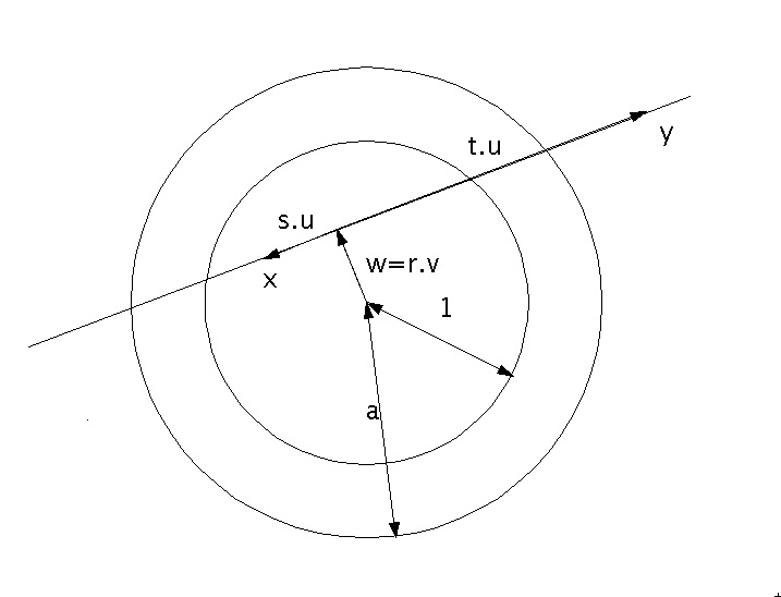
Figure 1. Parametrization by $r,s,t,u,v$

We reparametrise the integral in terms of $r,s,t,u,v$. We note that $(u,v)$ parametrize the unit tangent bundle $T_{1}({\bf S}^{n-2})$.

To calculate the Jacobian, we first change variables from $(x,y)$ to $(x,z)$ where $z=y-x$. Then the Jacobian is trivially equal to one. As $z=y-x=(t-s)u$, then from standard polar coordinates we have that

$$dV(z)=(t-s)^{n-2}d\Omega(u)d(t-s).$$

where $d\Omega(u)$ is the volume form on the unit sphere ${\bf S}^{n-2}$ in ${\bf R}^{n-1}$. Now for fixed $u$, then $x=s.u+r.v$ is in cylindrical polar coordinates with respect to $v$. We let $d\Omega(u,v)$ be the spherical volume form on the vectors perpendicular to $u$. Then as $u,v$ we have in terms of spherical polar coordinates

$$dV(x)=r^{n-3}d\Omega(u,v).dr.ds$$

$$dV(x)dV(y)=(t-s)^{n-2}r^{n-3}d\Omega(u,v)d\Omega(u)dr.ds.d(t-s).$$

Therefore

$$dV(x)dV(y)=(t-s)^{n-2}r^{n-3}d\Omega(u,v)d\Omega(u)dr.ds.dt.$$

We consider the vertical hyperbolic plane $P$ containing $x,y$. Then we see that $P$ intersects both $P_{0},P_{a}$ in semicircles centered about $w$. By definition of $r=|w|$ we have that the semicircles have radii $r_{1}=\sqrt{1-r^{2}},r_{2}=\sqrt{a^{2}-r^{2}}$ respectively. The geodesic with endpoints $x,y$ is contained in $P$. Therefore restricting to $P$ and scaling by $1/r_{1}$ we have that the length $L_{a}(x,y)$ is given by the previous lemma

$$L_{a}(x,y)=L_{\frac{r_{2}}{r_{1}}}\left(\frac{s}{r_{1}},\frac{t}{r_{1}}\right)=\frac{1}{2}\log\left(\frac{(t^{2}-r_{1}^{2})(s^{2}-r_{2}^{2})}{(t^{2}-r_{2}^{2})(s^{2}-r_{1}^{2})}\right).$$

Then we have

$$F_{n}(l)=\frac{2}{V_{n-1}}\int_{0}^{1}dr\int_{{\bf S}^{n-2}}d\Omega(u)\int_{{\bf S}^{n-3}}d\Omega(u,v)\int_{|s|<r_{1}}ds\int_{t>r_{2}}\frac{\log\left(\frac{(t^{2}-r_{1}^{2})(s^{2}-r_{2}^{2})}{(t^{2}-r_{2}^{2})(s^{2}-r_{1}^{2})}\right)}{(s-t)^{2n-2}}(t-s)^{n-2}r^{n-3}dt$$

Integrating over $u,v$ we get

$$F_{n}(l)=\frac{2V_{n-2}V_{n-3}}{V_{n-1}}\int_{0}^{1}r^{n-3}dr\int^{r_{1}}_{-r_{1}}ds\int_{t>r_{2}}\frac{\log\left(\frac{(t^{2}-r_{1}^{2})(s^{2}-r_{2}^{2})}{(t^{2}-r_{2}^{2})(s^{2}-r_{1}^{2})}\right)}{(t-s)^{n}}dt$$

We let $u=s/r_{1},v=t/r_{1}$ and $b=r_{2}/r_{1}$ then

$$F_{n}(l)=\frac{2V_{n-2}V_{n-3}}{V_{n-1}}\int_{0}^{1}r^{n-3}dr\left(\frac{1}{r_{1}^{n-2}}\int^{1}_{-1}du\int^{\infty}_{b}\frac{\log\left(\frac{(v^{2}-1)(u^{2}-b^{2})}{(v^{2}-b^{2})(u^{2}-1)}\right)}{(v-u)^{n}}dv\right)$$

We define

$$M_{n}(b)=\int^{1}_{-1}du\int^{\infty}_{b}\frac{\log\left(\frac{(v^{2}-1)(u^{2}-b^{2})}{(v^{2}-b^{2})(u^{2}-1)}\right)}{(v-u)^{n}}dv$$

Therefore

(1) $$F_{n}(l)=\frac{2V_{n-2}V_{n-3}}{V_{n-1}}\int_{0}^{1}\frac{r^{n-3}}{\left(\sqrt{1-r^{2}}\right)^{n-2}}.M_{n}\left(\sqrt{\frac{a^{2}-r^{2}}{1-r^{2}}}\right)dr.$$

We obtain an alternate integral form for $F_{n}$ by letting $x=\sqrt{\frac{a^{2}-r^{2}}{1-r^{2}}}$. then

$$x^{2}=\frac{a^{2}-r^{2}}{1-r^{2}}\qquad r^{2}=\frac{x^{2}-a^{2}}{x^{2}-1}\qquad 2rdr=\frac{(a^{2}-1)}{(x^{2}-1)^{2}}2xdx$$

Giving

$$r^{n-3}dr=r^{n-4}r.dr=\left(\frac{x^{2}-a^{2}}{x^{2}-1}\right)^{\frac{n}{2}-2}\left(\frac{a^{2}-1}{(x^{2}-1)^{2}}\right)xdx=\frac{x(a^{2}-1)(x^{2}-a^{2})^{\frac{n}{2}-2}}{(x^{2}-1)^{\frac{n}{2}}}dx$$

$$1-r^{2}=\frac{a^{2}-1}{x^{2}-1}\qquad\frac{1}{(\sqrt{1-r^{2}})^{n-2}}=\left(\frac{x^{2}-1}{a^{2}-1}\right)^{\frac{n}{2}-1}$$

Therefore

(2) $$F_{n}(l)=\frac{2V_{n-2}V_{n-3}}{V_{n-1}}\int_{a}^{\infty}\left(\frac{x^{2}-a^{2}}{a^{2}-1}\right)^{\frac{n}{2}-2}\left(\frac{xM_{n}(x)}{x^{2}-1}\right)dx$$

4.1. Formula For $M_{n}$

We give an explicit formula for $M_{n}$. in order to do so we first need to state some integral formulae. For $n\geq 1$ we define the polynomial function $P_{n}$ by

$$P_{n}(z)=\sum_{k=1}^{n}\frac{x^{k}}{k}.$$

We also define $P_{0}(z)=0$. We note that for $|x|<1$, $P_{n}(x)$ is the first $n$ terms of the Taylor series of $-\log(1-x)$. We therefore define the function $L_{n}(x)$ by $L_{n}(x)=\log|1-x|+P_{n}(x).$ For $|x|<1$ we have

$$L_{n}(x)=-\sum_{k=n+1}^{\infty}\frac{x^{k}}{k}.$$

We note that $L_{0}(x)=\log|1-x|$. We also note that $P_{n}(1)=1+\frac{1}{2}+\ldots+\frac{1}{n}$, the n^th Harmonic number.

Then we have the following integral formula.

Lemma 5.

If $a\neq b\in{\bf R}$ and $n$ a positive integer then

$$\int\frac{dx}{(x-a)(x-b)^{n}}\ =\ \frac{1}{(a-b)^{n}}\left(\log\left|\frac{x-a}{x-b}\right|+P_{n-1}\left(\frac{a-b}{x-b}\right)\right)=\frac{L_{n-1}\left(\frac{a-b}{x-b}\right)}{(a-b)^{n}}$$

Proof: We note that

$$\frac{1}{x^{n}(x-c)}=\frac{1}{c^{n}}\left(\frac{1}{x-c}-\frac{x^{n}-c^{n}}{x^{n}(x-c)}\right)=\frac{1}{c^{n}}\left(\frac{1}{x-c}-\frac{Q_{n-1}(x)}{x^{n}}\right)$$

where

$$Q_{n-1}(x)=\frac{x^{n}-c^{n}}{x-c}=\sum_{k=1}^{n}x^{k-1}c^{n-k}$$

Therefore

$$\int\frac{1}{x^{n}(x-c)}dx=\frac{1}{c^{n}}\left(\int\frac{dx}{x-c}-\int\frac{Q_{n-1}(x)}{x^{n}}dx\right)=\frac{1}{c^{n}}\left(\log|x-c|-\int\frac{Q_{n-1}(x)}{x^{n}}dx\right)$$

As

$$\frac{Q_{n-1}(x)}{x^{n}}=\sum_{k=1}^{n}\frac{c^{n-k}}{x^{n-k+1}}$$

then

$$\int\frac{Q_{n-1}(x)}{x^{n}}dx=\log|x|-\sum_{k=1}^{n-1}\frac{c^{n-k}}{(n-k).x^{n-k}}=\log|x|-P_{n-1}\left(\frac{c}{x}\right)$$

Therefore

$$\int\frac{1}{x^{n}(x-c)}dx=\frac{1}{c^{n}}\left(\log\left|\frac{x-c}{x}\right|+P_{n-1}\left(\frac{c}{x}\right)\right)=\frac{L_{n-1}\left(\frac{c}{x}\right)}{c^{n}}$$

The result now follows by elementary substitution.  

Integrating by parts we get,

Corollary 6.

For $n\geq 2$

$$\int\frac{\log|x-a|}{(x-b)^{n}}dx=\frac{1}{n-1}\left(\frac{L_{n-2}\left(\frac{a-b}{x-b}\right)}{(a-b)^{n-1}}-\frac{\log|x-a|}{(x-b)^{n-1}}\right)$$

Furthermore for $k\geq 1$

$$\lim_{x\rightarrow a}\left(\frac{\log|x-a|}{(b-x)^{k}}-\frac{L_{n}\left(\frac{b-a}{b-x}\right)}{(b-a)^{k}}\right)=\frac{\log|b-a|-P_{n}(1)}{(b-a)^{k}}$$

Lemma 7.

The function $M_{n}:(1,\infty)\rightarrow{\bf R}_{+}$ has the explicit form

$$M_{n}(b)=\frac{1}{(n-1)(n-2)}\left(\frac{1}{(b-1)^{n-2}}\left(\log(\frac{(b+1)^{2}}{(4b)})+2P_{n-2}(1)-L_{n-3}(\frac{b-1}{b+1})-(-1)^{n}L_{n-3}(\frac{-b+1}{b+1})\right)+\right.$$

$$\frac{1}{(b+1)^{n-2}}\left(-\log(\frac{(b-1)^{2}}{(4b)})-2P_{n-2}(1)+L_{n-3}(\frac{b+1}{b-1})+(-1)^{n}L_{n-3}(\frac{-b-1}{b-1})\right)+$$

$$\left.\frac{1}{(2b)^{n-2}}\left(L_{n-3}(\frac{2b}{b+1})-L_{n-3}(\frac{2b}{b-1})\right)+\frac{1}{2^{n-2}}\left(L_{n-3}(\frac{2}{b+1})-(-1)^{n}L_{n-3}(\frac{-2}{b-1}\right)\right)$$

Furthermore $M_{n}$ satisfies

$$\lim_{b\rightarrow 1^{+}}(b-1)^{n-2}M_{n}(b)=D_{n}=\frac{2P_{n-2}(1)}{(n-1)(n-2)}\qquad\mbox{and}\qquad\lim_{b\rightarrow\infty}\frac{b^{n-1}}{\log{b}}.M_{n}(b)=\frac{4}{n-1}.$$

Proof: We let

$$I(u,b)=\int^{\infty}_{b}\frac{\log\left(\frac{(v^{2}-1)(b^{2}-u^{2})}{(v^{2}-b^{2})(1-u^{2})}\right)}{(v-u)^{n}}dv$$

then $M_{n}(b)=\int_{0}^{1}I(u,b)du$. We split $I=I_{1}+I_{2}$ where

$$I_{1}(u,b)=\int^{\infty}_{b}\frac{\log\left(\frac{b-u}{v-b}\right)}{(v-u)^{n}}dv\qquad I_{2}(u,b)=\int^{\infty}_{b}\frac{\log\left(\frac{(v^{2}-1)(b+u)}{(v+b)(1-u^{2})}\right)}{(v-u)^{n}}dv.$$

By the above lemma,

$$I_{1}(u,b)=\left.\frac{1}{n-1}\left(\frac{\log(\frac{v-b}{b-u})}{(v-u)^{n-1}}-\frac{L_{n-2}\left(\frac{b-u}{v-u}\right)}{(b-u)^{n-1}}\right)\right|_{b}^{\infty}$$

Therefore by the above corollary

$$I_{1}(u,b)=\frac{1}{n-1}\left(\frac{P_{n-2}(1)}{(b-u)^{n-1}}\right)$$

$$I_{2}(u,b)=\left.\left(\frac{-1}{n-1}\right)\frac{\log\left(\frac{(v^{2}-1)(b+u)}{(v+b)(1-u^{2})}\right)}{(v-u)^{n-1}}\right|_{b}^{\infty}+\frac{1}{n-1}\int_{b}^{\infty}\frac{1}{(v-u)^{n-1}}\left(\frac{1}{v-1}+\frac{1}{v+1}-\frac{1}{v+b}\right)dv$$

Evaluating we get

$$I_{2}(u,b)=\frac{1}{n-1}\left(\frac{\log\left(\frac{(b^{2}-1)(b+u)}{(2b)(1-u^{2})}\right)}{(b-u)^{n-1}}+\int_{b}^{\infty}\frac{1}{(v-u)^{n-1}}\left(\frac{1}{v-1}+\frac{1}{v+1}-\frac{1}{v+b}\right)dv\right)$$

Therefore

$$M_{n}(b)=\frac{1}{n-1}\left(\int_{-1}^{1}\frac{\log\left(\frac{(b^{2}-1)(b+u)}{(2b)(1-u^{2})}\right)+P_{n-2}(1)}{(b-u)^{n-1}}du+\int_{-1}^{1}\int_{b}^{\infty}\frac{1}{(v-u)^{n-1}}\left(\frac{1}{v-1}+\frac{1}{v+1}-\frac{1}{v+b}\right)dvdu\right)$$

We once again split this integral as follows;

$$J_{1}(b)=\frac{1}{n-1}\left(\int_{-1}^{1}\frac{\log\left(\frac{(b^{2}-1)}{(2b)}\right)+P_{n-2}(1)}{(b-u)^{n-1}}du\right)$$

$$J_{2}(b)=\frac{1}{n-1}\left(\int_{-1}^{1}\frac{\log\left(\frac{b+u}{(1-u)(1+u)}\right)}{(b-u)^{n-1}}du\right)$$

$$J_{3}(b)=\frac{1}{n-1}\left(\int_{-1}^{1}\int_{b}^{\infty}\frac{1}{(v-u)^{n-1}}\left(\frac{1}{v-1}+\frac{1}{v+1}-\frac{1}{v+b}\right)dvdu\right)$$

We now evaluate each of $J_{1},J_{2},J_{3}$.

$J_{1}$: Integrating we get

$$J_{1}(b)=\frac{\log\left(\frac{(b^{2}-1)}{(2b)}\right)+P_{n-2}(1)}{(n-1)(n-2)}\left(\frac{1}{(b-1)^{n-2}}-\frac{1}{(b+1)^{n-2}}\right)$$

$J_{2}$: By the above lemma

$$J_{2}(b)=\left.\frac{1}{(n-1)(n-2)}\left(\frac{\log\left(\frac{b+u}{(1-u)(1+u)}\right)}{(b-u)^{n-2}}-\frac{L_{n-3}(\frac{2b}{b-u})}{(2b)^{n-2}}+\frac{L_{n-3}(\frac{b-1}{b-u})}{(b-1)^{n-2}}+\frac{L_{n-3}(\frac{b+1}{b-u})}{(b+1)^{n-2}}\right)\right|_{-1}^{1}$$

Therefore

$$(n-1)(n-2)J_{2}(b)=\left(\frac{\log(\frac{b+1}{2})-L_{n-3}(\frac{b-1}{b+1})}{(b-1)^{n-2}}\right)+\left(\frac{L_{n-3}(\frac{2b}{b+1})-L_{n-3}(\frac{2b}{b-1})}{(2b)^{n-2}}\right)+\left(\frac{-\log(\frac{b-1}{2})+L_{n-3}(\frac{b+1}{b-1})}{(b+1)^{n-2}}\right)+$$

$$\lim_{u\rightarrow 1-}\left(-\frac{\log(1-u)}{(b-u)^{n-2}}+\frac{L_{n-3}(\frac{b-1}{b-u})}{(b-1)^{n-2}}\right)+\lim_{u\rightarrow-1^{+}}\left(\frac{\log(1+u)}{(b-u)^{n-2}}-\frac{L_{n-3}(\frac{b+1}{b-u})}{(b+1)^{n-2}}\right)$$

By the corollary above

$$\lim_{u\rightarrow 1-}\left(-\frac{\log(1-u)}{(b-u)^{n-2}}+\frac{L_{n-3}(\frac{b-1}{b-u})}{(b-1)^{n-2}}\right)=\frac{P_{n-3}(1)-\log(b-1)}{(b-1)^{n-2}}$$

$$\lim_{u\rightarrow-1^{+}}\left(\frac{\log(1+u)}{(b-u)^{n-2}}-\frac{L_{n-3}(\frac{b+1}{b-u})}{(b+1)^{n-1}}\right)=\frac{\log(b+1)-P_{n-3}(1)}{(b+1)^{n-2}}$$

Therefore

$$(n-1)(n-2)J_{2}(b)=\left(\frac{\log(\frac{b+1}{2(b-1)})+P_{n-3}(1)-L_{n-3}(\frac{b-1}{b+1})}{(b-1)^{n-2}}\right)+\left(\frac{L_{n-3}(\frac{2b}{b+1})-L_{n-3}(\frac{2b}{b-1})}{(2b)^{n-2}}\right)$$

$$+\left(\frac{-\log(\frac{b-1}{2(b+1)})-P_{n-3}(1)+L_{n-3}(\frac{b+1}{b-1})}{(b+1)^{n-2}}\right)$$

$J_{3}$: Switching the order of integration we get

$$J_{3}(b)=\frac{1}{(n-1)(n-2)}\int_{b}^{\infty}\left(\frac{1}{v-1}+\frac{1}{v+1}-\frac{1}{v+b}\right)\left(\frac{1}{(v-1)^{n-2}}-\frac{1}{(v+1)^{n-2}}\right)dv$$

Therefore

$$J_{3}(b)=\frac{1}{(n-1)(n-2)}\left(\frac{\frac{1}{n-2}}{(b-1)^{n-2}}-\frac{\frac{1}{n-2}}{(b+1)^{n-2}}+\frac{L_{n-3}(\frac{2}{b+1})}{2^{n-2}}-\frac{L_{n-3}(\frac{-2}{b-1})}{(-2)^{n-2}}+\frac{L_{n-3}(\frac{-b-1}{b-1})}{(-b-1)^{n-2}}-\frac{L_{n-3}(\frac{-b+1}{b+1})}{(-b+1)^{n-2}}\right)$$

Combining $J_{1},J_{2},J_{3}$ we have

$$M_{n}(b)=\frac{1}{(n-1)(n-2)}\left(\left(\frac{\log\left(\frac{(b+1)^{2}}{4b}\right)+P_{n-2}(1)+P_{n-3}(1)-L_{n-3}(\frac{b-1}{b+1})+\frac{1}{n-2}-(-1)^{n}L_{n-3}(\frac{-b+1}{b+1})}{(b-1)^{n-2}}\right)+\right.$$

$$\left(\frac{-\log\left(\frac{(b-1)^{2}}{(4b)}\right)-P_{n-2}(1)-P_{n-3}(1)+L_{n-3}(\frac{b+1}{b-1})-\frac{1}{n-2}+(-1)^{n}L_{n-3}(\frac{-b-1}{b-1})}{(b+1)^{n-2}}\right)+$$

$$\left.\left(\frac{\frac{1}{b^{n-2}}(L_{n-3}(\frac{2b}{b+1})-L_{n-3}(\frac{2b}{b-1}))+L_{n-3}(\frac{2}{b+1})-(-1)^{n}L_{n-3}(\frac{-2}{b-1})}{2^{n-2}}\right)\right)$$

Noting that $P_{n-3}(1)+\frac{1}{n-2}=P_{n-2}(1)$ we simplify to get

$$M_{n}(b)=\frac{1}{(n-1)(n-2)}\left(\frac{1}{(b-1)^{n-2}}\left(\log(\frac{(b+1)^{2}}{(4b)})+2P_{n-2}(1)-L_{n-3}(\frac{b-1}{b+1})-(-1)^{n}L_{n-3}(\frac{-b+1}{b+1})\right)\right.$$

$$+\frac{1}{(b+1)^{n-2}}\left(-\log(\frac{(b-1)^{2}}{(4b)})-2P_{n-2}(1)+L_{n-3}(\frac{b+1}{b-1})+(-1)^{n}L_{n-3}(\frac{-b-1}{b-1})\right)$$

$$+\left.\frac{1}{(2b)^{n-2}}\left(L_{n-3}(\frac{2b}{b+1})-L_{n-3}(\frac{2b}{b-1})\right)+\frac{1}{2^{n-2}}\left(L_{n-3}(\frac{2}{b+1})-(-1)^{n}L_{n-3}(\frac{-2}{b-1}\right)\right)$$

It follows from the above directly that $M_{n}$ satisfies

$$\lim_{b\rightarrow 1^{+}}(b-1)^{n-2}M_{n}(b)=\frac{2P_{n-2}(1)}{(n-1)(n-2)}.$$

We now consider the limit as $b$ tends to infinity. As $L_{n-3}$ is continuous except at $x=1$, we replace the $L_{n-3}$ terms by the limiting value if the argument does not tend to 1 or is infinite. For other values we substitute $P_{n}(x)=\log|1-x|+P_{n}(x)$ and collect terms. Therefore

$$\lim_{b\rightarrow\infty}(b-1)^{n-2}M_{n}(b)=\frac{1}{(n-1)(n-2)}\lim_{b\rightarrow\infty}\left(\left(-\log(4)+2P_{n-2}(1)-\log(\frac{2}{b+1})-P_{n-3}(1)-(-1)^{n}L_{n-3}(-1)\right)\right.$$

$$+\left(\log(4)-2P_{n-2}(1)+\log(\frac{2}{b-1})+P_{n-3}(1)+(-1)^{n}L_{n-3}(-1)\right)$$

$$+\left.\frac{1}{2^{n-2}}\left(L_{n-3}(2)-L_{n-3}(2)\right)+\frac{(b-1)^{n-2}}{2^{n-2}}\left(L_{n-3}(\frac{2}{b+1})-(-1)^{n}L_{n-3}(\frac{-2}{b-1}\right)\right)$$

After cancellation we have

$$\lim_{b\rightarrow 1^{+}}(b-1)^{n-2}M_{n}(b)=\frac{1}{(n-1)(n-2)}\lim_{b\rightarrow\infty}\frac{(b-1)^{n-2}}{2^{n-2}}\left(L_{n-3}(\frac{2}{b+1})-(-1)^{n}L_{n-3}(\frac{-2}{b-1}\right).$$

For $b$ large we can use the Taylor series expansion for $L_{n-3}$ to get

$$L_{n-3}\left(\frac{2}{b+1}\right)=\frac{1}{n-2}\left(\frac{2}{b+1}\right)^{n-2}+\epsilon_{1}.\left(\frac{2}{b+1}\right)^{n-3}\qquad L_{n-3}\left(\frac{-2}{b-1}\right)=\frac{1}{n-2}\left(\frac{-2}{b-1}\right)^{n-2}+\epsilon_{2}.\left(\frac{-2}{b-1}\right)^{n-3}$$

Therefore

$$\lim_{b\rightarrow\infty}\frac{(b-1)^{n-2}}{2^{n-2}}\left(L_{n-3}(\frac{2}{b+1})-(-1)^{n}L_{n-3}(\frac{-2}{b-1})\right)=$$

$$\lim_{b\rightarrow\infty}\left(\frac{1}{n-2}+\epsilon_{1}\left(\frac{2}{b+1}\right)-(-1)^{n}\left(\frac{(-1)^{n-2}}{n-2}+\epsilon_{2}\frac{(-1)^{n-2}.-2}{b-1}\right)\right)=0$$

We now use this fact to show the exact asyptotic behavior of $M_{n}(b)$ as $b$ tends to infinity. From the above we have

$$\lim_{b\rightarrow\infty}b^{n-2}M_{n}(b)=0.$$

We now expand $M_{n}(b)$ around infinity by writing as a Taylor series in $1/b$. From the form of $M_{n}$ we must therefore have that for large $b$

$$M_{n}(b)=\frac{c_{0}+d_{0}\log{b}}{b^{n-1}}+\frac{c_{1}+d_{1}\log{b}}{b^{n}}+\ldots$$

Thus we have that the leading terms is

$$M_{n}(b)\simeq\frac{d_{0}\log{b}}{b^{n-1}}\qquad\mbox{ or }\qquad\lim_{b\rightarrow\infty}b^{n-1}\log{b}.M_{n}(b)=d_{0}.$$

To find $d_{0}$ we need only gather the $\log{b}$ terms. We can replace terms of the form $\log(sb+t)$ by $\log{b}$ and also can ignore terms $L_{n-3}(m(b))$ where $m(b)$ does not tend to $1$ as $b$ tends to infinity. Therefore

$$M_{n}(b)\simeq\frac{1}{(n-1)(n-2)}\left(\frac{2\log{b}}{(b-1)^{n-2}}-\frac{2\log{b}}{(b+1)^{n-2}}\right)\simeq\frac{1}{(n-1)(n-2)}\frac{2\log{b}}{b^{n-2}}\left(\frac{1}{(1-1/b)^{n-2}}-\frac{1}{(1+1/b)^{n-2}}\right)$$

Therefore

$$M_{n}(b)\simeq\frac{1}{(n-1)(n-2)}\frac{2\log{b}}{b^{n-2}}\left(1+(n-2)\frac{1}{b}-\left(1-(n-2)\frac{1}{b}\right)\right)=\left(\frac{4}{n-1}\right)\frac{\log{b}}{b^{n-1}}.$$

 

Corollary 8.

For $n$ even there is a closed form for $F_{n}$.

Proof: We note by equation 2, for all $n$ we have

$$F_{n}(l)=\frac{2V_{n-2}V_{n-3}}{V_{n-1}}\int_{a}^{\infty}\left(\frac{x^{2}-a^{2}}{a^{2}-1}\right)^{\frac{n}{2}-2}\left(\frac{xM_{n}(x)}{x^{2}-1}\right)dx.$$

By the above lemma, $M_{n}$ is in terms of rational functions and rational functions times sums of linear log functions $\log(a+bx)$. Therefore for $n$ even the function to be integrated in the above equation for $F_{n}$ is a sum of rational functions and rational functions times linear log functions. As such functions have explicit formulae, we can therefore find formulae for $F_{n}$ for $n$ even. As the number of terms of $M_{n}$ is linear in $n$ we obtain approximately a quadratic number of terms for $F_{n}$.  

4.2. Three-dimensional case

For $n=3$ we have

$$F_{3}(l)=2.\int_{0}^{1}\frac{M_{3}\left(\sqrt{\frac{a^{2}-r^{2}}{1-r^{2}}}\right)}{\sqrt{1-r^{2}}}.dr.$$

Using the above formula we have that

$$M_{3}(x)=\frac{2}{x^{2}-1}(1-\log(2))-\frac{1}{2x}\left(\frac{x-1}{x+1}\right)\log(x-1)+\frac{1}{2x}\left(\frac{x+1}{x-1}\right)\log(x+1)$$

Also we have

$$M_{3}(x)\simeq\frac{1}{x-1}$$

for $x$ close to 1.

4.3. Four-dimensional case

For $n=4$ we have

$$F_{4}(l)=8.\int_{0}^{1}\frac{r.M_{4}\left(\sqrt{\frac{a^{2}-r^{2}}{1-r^{2}}}\right)}{1-r^{2}}.dr.$$

Using the above formula we have that

$$M_{4}(b)=\frac{1}{6}\left(\frac{3+2\log(\frac{(b+1)^{2}}{4b})}{(b-1)^{2}}-\frac{3+2\log(\frac{(b-1)^{2}}{4b})}{(b+1)^{2}}+\frac{\log(\frac{b-1}{b+1})+\frac{b}{b+1}-\frac{b}{b-1}}{2b^{2}}+\frac{\log(\frac{b-1}{b+1})+\frac{1}{b+1}+\frac{1}{b-1}}{2}\right)$$

Also we have

$$M_{4}(x)\simeq\frac{1}{2}\frac{1}{(x-1)^{2}}$$

for $x$ close to 1.

5. Properties of $F_{n}$

We now describe the properties of $F_{n}$. In particular we complete the proof of Theorem 1.

Lemma 9.

The function $F_{n}$ satisfies the following:

1. There exists a $C_{n}>0$ such that

   $$F_{n}(l)\leq\frac{C_{n}}{(e^{l}-1)^{n-2}}$$

2. $F_{n}$ is continuous monotonically decreasing

3. $$\lim_{l\rightarrow 0}l^{n-2}F_{n}(l)=K_{n}=\frac{2\pi^{\frac{n-3}{2}}P_{n-2}(1)\Gamma(\frac{n}{2}+1)\Gamma(\frac{n}{2}-1)}{n.\Gamma(\frac{n+1}{2})\Gamma(n-1)}$$

4. $$\lim_{l\rightarrow\infty}\frac{e^{(n-1)l}}{l}.F_{n}(l)=\frac{(n-2)\pi^{\frac{n-2}{2}}\Gamma(\frac{n}{2}-1)}{(\Gamma(\frac{n+1}{2}))^{2}}$$

Proof:

1. For $a=e^{l}$ we have

   $$F_{n}(l)=\frac{2V_{n-2}V_{n-3}}{V_{n-1}}\int_{0}^{1}\frac{r^{n-3}}{\left(\sqrt{1-r^{2}}\right)^{n-2}}.M_{n}\left(\sqrt{\frac{a^{2}-r^{2}}{1-r^{2}}}\right)dr$$

   with

   $$M_{n}(b)=\int_{-1}^{1}ds\int_{b}^{\infty}\frac{\log\left(\frac{(t^{2}-1)(s^{2}-b^{2})}{(t^{2}-b^{2})(s^{2}-1)}\right)}{(t-s)^{n}}dt.$$

   By lemma 7 we have that there exists a $B_{n}>0$ such that

   $$M_{n}(x)\leq\frac{B_{n}}{(x-1)^{n-2}}.$$

   Therefore

   $$F_{n}(l)\leq\frac{2B_{n}V_{n-2}V_{n-3}}{V_{n-1}}\int_{0}^{1}\frac{r^{n-3}}{\left(\sqrt{1-r^{2}}\right)^{n-2}.\left(\sqrt{\frac{a^{2}-r^{2}}{1-r^{2}}}-1\right)^{n-2}}dr.$$

   $$F_{n}(l)\leq\frac{2B_{n}V_{n-2}V_{n-3}}{V_{n-1}}\int_{0}^{1}\frac{r^{n-3}}{\left(\sqrt{a^{2}-r^{2}}-\sqrt{1-r^{2}}\right)^{n-2}}dr.$$

   Rationalizing the denominator we get

   $$F_{n}(l)\leq\frac{2B_{n}V_{n-2}V_{n-3}}{V_{n-1}}\int_{0}^{1}\frac{r^{n-3}(\sqrt{a^{2}-r^{2}}+\sqrt{1-r^{2}})^{n-2}}{(a^{2}-1)^{n-2}}dr.$$

   Therefore

   $$(a-1)^{n-2}F_{n}(l)\leq\frac{2B_{n}V_{n-2}V_{n-3}}{V_{n-1}}\int_{0}^{1}r^{n-3}\left(\frac{\sqrt{a^{2}-r^{2}}+\sqrt{1-r^{2}}}{a+1}\right)^{n-2}dr.$$

   We have for $a\geq 0,0\leq r\leq 1$

   $$0\leq\frac{\sqrt{a^{2}-r^{2}}+\sqrt{1-r^{2}}}{a+1}\leq 1.$$

   Therefore we have a $C_{n}>0$ such that

   $$(e^{l}-1)^{n-2}F_{n}(l)\leq C_{n}\qquad\mbox{ giving }\qquad F_{n}(l)\leq\frac{C_{n}}{(e^{l}-1)^{n-2}}.$$

2. We have for $a=e^{l}$ then by equation 2,

   $$F_{n}(l)=\frac{2V_{n-2}V_{n-3}}{V_{n-1}}\int_{a}^{\infty}\left(\frac{x^{2}-a^{2}}{a^{2}-1}\right)^{\frac{n}{2}-2}\left(\frac{xM_{n}(x)}{x^{2}-1}\right)dx.$$

   The function $\frac{x^{2}-a^{2}}{a^{2}-1}$ is monotonically decreasing in $a$. Therefore for $n\geq 4$ then $\frac{n}{2}-2\geq 0$ and if $a<b$

   $$\int_{b}^{\infty}\left(\frac{x^{2}-b^{2}}{b^{2}-1}\right)^{\frac{n}{2}-2}\left(\frac{xM_{n}(x)}{x^{2}-1}\right)dx\leq\int_{b}^{\infty}\left(\frac{x^{2}-a^{2}}{a^{2}-1}\right)^{\frac{n}{2}-2}\left(\frac{xM_{n}(x)}{x^{2}-1}\right)dx\leq\int_{a}^{\infty}\left(\frac{x^{2}-a^{2}}{a^{2}-1}\right)^{\frac{n}{2}-2}\left(\frac{xM_{n}(x)}{x^{2}-1}\right)dx$$

   Thus $F_{n}$ is monotonic for $n\geq 4$. The case for $n=3$ we have an explicit form for $M_{3}$ given by

   $$M_{3}(x)=\frac{2}{x^{2}-1}(1-\log(2))-\frac{1}{2x}\left(\frac{x-1}{x+1}\right)\log(x-1)+\frac{1}{2x}\left(\frac{x+1}{x-1}\right)\log(x+1).$$

   This function is monotonically decreasing. As

   $$F_{3}(l)=2.\int_{0}^{1}\frac{M_{3}\left(\sqrt{\frac{a^{2}-r^{2}}{1-r^{2}}}\right)}{\sqrt{1-r^{2}}}.dr$$

   then it follows that $F_{3}$ is also monotonically decreasing.

3. We now analyse the behavior of $F_{n}(l)$ as $l$ tends to zero. By lemma 7 we have that

   $$\lim_{b\rightarrow 1^{+}}(b-1)^{n-2}M_{n}(b)=D_{n}$$

   . Let $\epsilon>0$. then on $[0,1-\epsilon]$ we have

   $$\lim_{a\rightarrow 1^{+}}\left(\sqrt{\frac{a^{2}-r^{2}}{1-r^{2}}}-1\right)^{n-2}M_{n}\left(\sqrt{\frac{a^{2}-r^{2}}{1-r^{2}}}\right)=D_{n}\qquad\mbox{uniformly}.$$

   Simplifying we have

   $$\left(\sqrt{\frac{a^{2}-r^{2}}{1-r^{2}}}-1\right)^{n-2}=\frac{(a^{2}-1)^{n-2}}{(\sqrt{a^{2}-r^{2}}+\sqrt{1-r^{2}})(\sqrt{1-r^{2}})^{n-2}}$$

   Therefore we have

   $$\lim_{a\rightarrow 1^{+}}(a-1)^{n-2}M_{n}\left(\sqrt{\frac{a^{2}-r^{2}}{1-r^{2}}}\right)=D_{n}.(1-r^{2})^{n-2}\qquad\mbox{uniformly on }r\in[1,1-\epsilon].$$

   Therefore

   $$\lim_{a\rightarrow 1^{+}}(a-1)^{n-2}\int_{0}^{1-\epsilon}\frac{r^{n-3}}{\left(\sqrt{1-r^{2}}\right)^{n-2}}.M_{n}\left(\sqrt{\frac{a^{2}-r^{2}}{1-r^{2}}}\right)dr=D_{n}.\int_{0}^{1-\epsilon}r^{n-3}(\sqrt{1-r^{2}})^{n-2}dr$$

   As $M_{n}(x)\leq\frac{B_{n}}{(x-1)^{n-2}}$ we have as above that

   $$\lim_{a\rightarrow 1^{+}}(a-1)^{n-2}\int_{1-\epsilon}^{1}\frac{r^{n-3}}{\left(\sqrt{1-r^{2}}\right)^{n-2}}.M_{n}\left(\sqrt{\frac{a^{2}-r^{2}}{1-r^{2}}}\right)dr\leq B_{n}\int_{1-\epsilon}^{1}r^{n-3}dr\leq B_{n}.\epsilon.$$

   Also for $n\geq 3$

   $$\int_{1-\epsilon}^{1}r^{n-3}(\sqrt{1-r^{2}})^{n-2}dr\leq\epsilon.$$

   Therefore

   $$\limsup_{a\rightarrow 1^{+}}\left|(a-1)^{n-2}\int_{0}^{1}\frac{r^{n-3}}{\left(\sqrt{1-r^{2}}\right)^{n-2}}.M_{n}\left(\sqrt{\frac{a^{2}-r^{2}}{1-r^{2}}}\right)dr-D_{n}.\int_{0}^{1}r^{n-3}(\sqrt{1-r^{2}})^{n-2}dr\right|\leq(B_{n}+D_{n})\epsilon.$$

   As $\epsilon$ is arbitrary we have

   $$\lim_{l\rightarrow 0^{+}}l^{n-2}F_{n}(l)=\lim_{a\rightarrow a^{+}}(a-1)^{n-2}F_{n}(l)=\frac{2V_{n-2}V_{n-3}D_{n}}{V_{n-1}}.\int_{0}^{1}r^{n-3}(\sqrt{1-r^{2}})^{n-2}dr.$$

   Substituting $x=r^{2}$, and letting $B$ be the Beta function then

   $$\int_{0}^{1}r^{n-3}(\sqrt{1-r^{2}})^{n-2}dr=\frac{1}{2}\int_{0}^{1}x^{\frac{n}{2}-2}(1-x)^{\frac{n}{2}-1}dx=\frac{1}{2}B(\frac{n}{2}-1,\frac{n}{2})=\frac{\Gamma(\frac{n}{2}-1).\Gamma(\frac{n}{2})}{2.\Gamma(n-1)}$$

   Combining we get

   $$\lim_{l\rightarrow 0^{+}}l^{n-2}F_{n}(l)=\frac{D_{n}.V_{n-2}V_{n-3}\Gamma(\frac{n}{2}-1).\Gamma(\frac{n}{2})}{V_{n-1}.\Gamma(n-1)}$$

   As the volume formula for the $n-$sphere is

   $$V_{n}=\frac{(n+1)\pi^{\frac{n+1}{2}}}{\Gamma(\frac{n+3}{2})}$$

   $$\lim_{l\rightarrow 0^{+}}l^{n-2}F_{n}(l)=K_{n}=\frac{2\pi^{\frac{n-3}{2}}P_{n-2}(1)\Gamma(\frac{n}{2}+1)\Gamma(\frac{n}{2}-1)}{n.\Gamma(\frac{n+1}{2})\Gamma(n-1)}$$

   We calculate $K_{n}$ for some small values. Starting with $n=3$ the first 10 values of $K_{n}$ are

   $$\frac{\pi}{2},1,\frac{11\pi^{2}}{192},\frac{5\pi}{54},\frac{137\pi^{3}}{30720},\frac{7\pi^{2}}{1125},\frac{121\pi^{4}}{458752},\frac{761\pi^{3}}{2315250},\frac{7129\pi^{5}}{566231040},\frac{1342\pi^{4}}{93767625},\ldots$$

4. We now consider $F_{n}(l)$ for $l$ large. Then for large $a$ as $(a^{2}-r^{2})/(1-r^{2})>a^{2}-1$ for $0<r<1$, and we have that

   $$\lim_{a\rightarrow\infty}\frac{\left(\sqrt{\frac{a^{2}-r^{2}}{1-r^{2}}}\right)^{n-1}}{\log\left(\sqrt{\frac{a^{2}-r^{2}}{1-r^{2}}}\right)}M_{n}\left(\sqrt{\frac{a^{2}-r^{2}}{1-r^{2}}}\right)=\frac{4}{n-1}\qquad\mbox{uniformly on }[0,1].$$

   Therefore on the interval $[0,1-\epsilon]$ we have

   $$\lim_{a\rightarrow\infty}\frac{a^{n-1}}{\log{a}}M_{n}\left(\sqrt{\frac{a^{2}-r^{2}}{1-r^{2}}}\right)=\frac{4}{n-1}.(\sqrt{1-r^{2}})^{n-1}\qquad\mbox{uniformly on }[0,1-\epsilon].$$

   Therefore

   $$\lim_{a\rightarrow\infty}\frac{a^{n-1}}{\log{a}}\int_{0}^{1-\epsilon}\frac{r^{n-3}}{(\sqrt{1-r^{2}})^{n-2}}.M_{n}\left(\sqrt{\frac{a^{2}-r^{2}}{1-r^{2}}}\right)dr=\frac{4}{n-1}\int_{0}^{1-\epsilon}r^{n-3}\sqrt{1-r^{2}}dr$$

   As this holds for all $\epsilon$, the improper integral exists and we have

   $$\lim_{a\rightarrow\infty}\frac{a^{n-1}}{\log{a}}\int_{0}^{1}\frac{r^{n-3}}{(\sqrt{1-r^{2}})^{n-2}}.M_{n}\left(\sqrt{\frac{a^{2}-r^{2}}{1-r^{2}}}\right)dr=\frac{4}{n-1}\int_{0}^{1}r^{n-3}\sqrt{1-r^{2}}dr=\frac{\sqrt{\pi}\Gamma(\frac{n}{2}-1)}{\Gamma(\frac{n+1}{2}).(n-1)}$$

   Therefore

   $$\lim_{l\rightarrow\infty}\frac{e^{(n-1)l}}{l}F_{n}(l)=\frac{2V_{n-2}V_{n-3}}{V_{n-1}}.\frac{\sqrt{\pi}\Gamma(\frac{n}{2}-1)}{\Gamma(\frac{n+1}{2}).(n-1)}=\frac{(n-2)\pi^{\frac{n-2}{2}}\Gamma(\frac{n}{2}-1)}{(\Gamma(\frac{n+1}{2}))^{2}}$$

 
The above lemma completes the proof of Theorem 1.

6. Volume Bounds

As an application of the above, we now consider lower bounds on volume for hyperbolic manifolds with totally geodesic boundary. Immediately from the monotonicity of $F_{n}$ we have the following;

Lemma 10.

If $M$ is a finite volume hyperbolic manifold with totally geodesic boundary with shortest orthogeodesic of length $l$ then

$$Vol_{n}(M)\geq F_{n}(l).$$

In the paper [6], Miyamoto studies volumes of hyperbolic manifolds with totally geodesic boundary using the length shortest return path from the boundary to itself, which in terms of orthogeodesics, is twice the length shortest orthogeodesic. Using packing methods for neighborhoods of boundary components he obtains the following result.

Theorem 11.

(Miyamoto [6]) There exists a function $\rho_{n}:{\bf R}_{+}\rightarrow{\bf R}_{+}$ such that if $M$ is a finite volume hyperbolic manifold with totally geodesic boundary with shortest orthogeodesic of length $l$ then

$$Vol_{n}(M)\geq\rho_{n}(l).Vol_{n-1}(\partial M)$$

with equality if and only if M is decomposed into truncated regular simplices of edge-length $2l$. Furthermore the function $\rho_{n}$ is monotonically increasing with $\rho_{n}(0)>0$ giving

$$Vol_{n}(M)\geq\rho_{n}(0).Vol_{n-1}(\partial M).$$

We note that these bounds are quite different as functions of $l$ as $F_{n}(l)$ tends to infinity as $l\rightarrow 0$ while $\rho_{n}(l)$ tends to a finite value. Also the lower bound of Miyamoto is proportional to the volume of the boundary while the bound given by $F_{n}$ gives no obvious relation.

We now use the asymptotic behavior of $F_{n}$ to get bounds on the volume of a hyperbolic n-manifold with geodesic boundary in terms of the volume of the boundary similar to the bound of Miyamoto. We first describe the volume of an $r$-neighborhood of a boundary component in terms of $r$.

Lemma 12.

Let $X$ be a finite volume subset of ${\bf H}^{n-1}\subseteq{\bf H}^{n}$. Let $N^{+}_{r}(X)$ be a one sided $r$-neighborhood of $X$ in ${\bf H}^{n}$. Then

$$\mbox{Vol}_{n}(N^{+}_{r}(X))=\mbox{Vol}_{n-1}(X).S_{n}(r)$$

where

$$S_{n}(r)=\int_{0}^{r}\cosh^{n-1}(x)\ dx.$$

Proof: We consider $X$ on the vertical hyperplane $P$ in the upper half-space model of ${\bf H}^{n}$ given by $x_{1}=0$. Then by elementary hyperbolic geometry the boundary of $N_{r}^{+}(P)$ is the Euclidean plane $x_{n}=\tan(\theta_{0}).x_{1}$ for $\theta_{0}$ satisfying $\sinh{r}=\tan{\theta_{0}}$.

We let $x_{1}=r\sin{\theta},x_{n}=r\cos{\theta}$. Then $(r,\theta,x_{2},\ldots,x_{n-1})\in N_{r}^{+}(X)$ if and only if $(0,x_{2},x_{3},\ldots,r)\in X$ and $0<\theta<\theta_{0}$. Changing variables we get

$$\mbox{Vol}_{n}(N^{+}_{r}(X))=\int_{N^{+}_{r}(X)}\frac{dx_{1}dx_{2}\ldots dx_{n}}{x^{n}_{n}}=\int_{N^{+}_{r}(X)}\frac{rd\theta drdx_{2}\ldots dx_{n-1}}{r^{n}\cos^{n}{\theta}}=$$

$$\int_{X}\frac{dx_{2}\ldots dx_{n-1}dr}{r^{n-1}}.\int_{0}^{\theta_{0}}\frac{d\theta}{\cos^{n}{\theta}}.$$

As $x_{n}=r$ on $P$ we get

$$\mbox{Vol}_{n}(N^{+}_{r}(X))=\int_{X}\frac{dx_{2}\ldots dx_{n-1}dx_{n}}{x_{n}^{n-1}}.\int_{0}^{\theta_{0}}\frac{d\theta}{\cos^{n}{\theta}}=\mbox{Vol}_{n-1}(X).\int_{0}^{\theta_{0}}\frac{d\theta}{\cos^{n}{\theta}}.$$

Therefore

$$\mbox{Vol}_{n}(N^{+}_{r}(X))=\mbox{Vol}_{n-1}(X).S_{n}(r)$$

where

$$S_{n}(r)=\int_{0}^{\theta_{0}}\sec^{n}{\theta}\ d\theta$$

for $\sinh{r}=\tan{\theta_{0}}$. We let $\sinh{x}=\tan{\theta}$ then $\cosh{x}dx=\sec^{2}{\theta}d\theta$. As $\cosh{x}=\sec{\theta}$ we have $dx=\sec{\theta}d\theta$ and

$$S_{n}(r)=\int_{0}^{\theta_{0}}\sec^{n}{\theta}\ d\theta=\int_{0}^{\theta_{0}}\sec^{n-1}(\theta)\sec{\theta}d\theta=\int_{0}^{r}\cosh^{n-1}(x)dx.$$

 

We now prove Theorem 2. We first restate the theorem.
Theorem 2. For $n\geq 3$, there exists a monotonically increasing function $H_{n}:{\bf R}_{+}\rightarrow{\bf R}_{+}$ and a constant $C_{n}>0$ such that if $M$ is a hyperbolic n-manifold with totally geodesic boundary of area $A$ then

$$\mbox{Vol}_{n}(M)\geq H_{n}(A)\geq C_{n}.A^{\left(\frac{n-2}{n-1}\right)}$$

Proof: We let $A=\mbox{Vol}_{n-1}(\partial M)$. We consider taking $\delta$ neighborhoods of $\partial M$ in $M$ denoted $N_{\delta}(\partial M)$. We let $\delta_{0}>0$ be the largest values such that the interior of $N_{\delta}(\partial M)$ is embedded. Then $M$ has an orthogeodesic $\alpha$ of length $d\leq 2\delta_{0}$ . Therefore there are two contributions to the volume, one part $V_{1}$ from the volume of the region associated with the orthogeodesic $\alpha$, and the other $V_{2}$ from the neighborhood of the boundary with $\mbox{Vol}_{n}(M)\geq\max(V_{1},V_{2}).$ Then we have $V_{1}=F_{n}(d)$ and as $F_{n}$ is monotonically decreasing $V_{1}\geq F_{n}(2\delta_{0})$. As $V_{2}$ is the (one-sided) $\delta_{0}$ neighborhood of $\partial M$, by lemma 12 we have

$$V_{2}=A.S_{n}(\delta_{0}).$$

We note that for small $x$, we have the simple approximation $S_{n}(x)\simeq x$, with $S_{n}(x)\geq\sinh{x}$ for all $x>0$. Also by the formula for $S_{n}$, we have that $S_{n}$ is convex.

By lemma 9, we have that $F_{n}$ is a continuous monotonically decreasing positive function that tends to zero at infinity and tends to infinity at $0$. We consider the continuous positive function $G_{n}(r)=\max(F_{n}(2r),A.S_{n}(r))$. Then $G_{n}$ has a positive minimum value depending only on $n$ and $A$ denoted $H_{n}(A)$. As $F_{n}$ is monotonically decreasing and $S_{n}$ monotonically increasing, we have that $H_{n}=J^{-1}$, where $J$ is the function

$$J(x)=\frac{F_{n}(2x)}{S_{n}(x)}.$$

We also note that $H_{n}(A)$ is the common value of the functions $F_{n}(2r),A.S_{n}(r)$ at their unique intersection point (see figure 2).

Therefore we have $\mbox{Vol}_{n}(M)\geq G_{n}(\delta_{0})\geq H_{n}(A)$. Obviously as $V_{2}$ is monotonic in volume, the function $H_{n}(A)$ is monotonic increasing in $A$ (see figure 2).

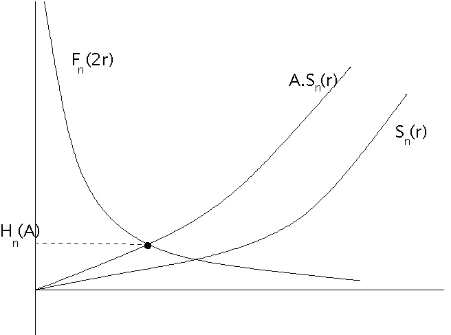
Figure 2. Graph of $G_{n}(r)$

By lemma 9, there is a $K_{n}>0$ such that

$$\lim_{l\rightarrow 0^{+}}l^{n-2}F_{n}(l)=K_{n}.$$

Therefore there is a $k_{n}$ such that for $l<1$

$$F_{n}(r)\geq\frac{k_{n}}{r^{n-2}}=f_{n}(r).$$

Also we have that $S_{n}(r)\geq A.r=s_{n}(r)$ for all $r$. We consider the equation $f_{n}(2x)=s_{n}(x)$. This has a unique solution

$$\frac{k_{n}}{2^{n-2}.x^{n-2}}=A.x\qquad x=\left(\frac{k_{n}}{2^{n-2}A}\right)^{1/(n-1)}=\frac{k^{\prime}_{n}}{A^{1/(n-1)}}$$

If $x<.5$ then we have for $r\leq x$ then $F_{n}(2r)\geq f_{n}(2r)\geq f_{n}(2x)$. Therefore $G_{n}(r)\geq f_{n}(2x)$ for $r\leq x$. Also for $r>x$ then $S_{n}(r)\geq s_{n}(r)\geq s_{n}(x)$. Therefore $G_{n}(r)\geq s_{n}(x)$ for $r>x$. Thus as $f_{n}(2x)=s_{n}(x)$ then $G_{n}(r)\geq s_{n}(x)$. Thus $H_{n}(A)\geq s_{n}(x)$ giving

$$H_{n}(A)\geq A.x=A.\frac{k^{\prime}_{n}}{A^{1/(n-1)}}=k^{\prime}_{n}A^{\frac{n-2}{n-1}}$$

If $x\geq.5$ then we have by monotonicity of $f_{n},s_{n}$, that $f_{n}(1)\geq s_{n}(.5)$. Therefore for $r\geq.5$ $S_{n}(r)\geq s_{n}(r)\geq s_{n}(.5)$. Therefore $G_{n}(r)\geq s_{n}(.5)$ for $r\geq.5$. If $r<.5$ then $F_{n}(2r)\geq f_{n}(2r)\geq f_{n}(1)\geq s_{n}(.5)$. Therefore $G_{n}(r)\geq s_{n}(.5)$ for $r\leq.5$. Thus $G_{n}(r)\geq s_{n}(.5)$ for all $r$. Thus $H_{n}(A)\geq s_{n}(.5)=A/2$ giving

$$H_{n}(A)\geq\frac{1}{2}.A=C_{n}.A$$

 

We note that using the approximation $F_{n}(x)=\frac{K_{n}}{x^{n-2}}$ for $x$ small we get the approximate bound of

$$H_{n}(A)\stackrel{{\scriptstyle\sim}}{{\geq}}\left(\frac{K_{n}.A}{2}\right)^{\frac{n-2}{n-1}}.$$

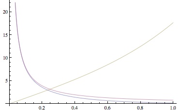
Figure 3. Graph of $F_{3}(2x)$, $\frac{\pi}{4x}$ and $4\pi S_{3}(x)$

7. General lower bound Examples

As the function $H_{n}(A)$ is monotonically increasing in $A$, if we have a general lower bound on the volume of a closed hyperbolic $n-$manifold then we obtain a lower bound for a hyperbolic $(n+1)-$manifold with geodesic boundary.

Hyperbolic 3-manifolds
In [5], Kojima and Miyamoto showed that the lowest volume hyperbolic three manifold with totally geodesic boundary has boundary a genus two surface and volume 6.452. Therefore $6.452$ is the best general lower bound.

By the above lemma 9, $F_{3}(x)\simeq\frac{\pi}{2x}$ for small $x$. Graphing $F_{3}$ we see that this approximation is very close (see figure 3).

For comparison with Kojima and Miyamoto, we note that as a closed hyperbolic surface has area at least $4\pi$, our methods give a lower bound of $H_{3}(4\pi)$ for the volume of a hyperbolic three-manifold with totally geodesic boundary. Plotting $F_{3}(2x)$ and $4\pi.S_{3}(x)$ we see that $H_{3}(4\pi)\approx 2.986$ (see figure 3).

References

[1]
M. Bridgeman,
Orthospectra of Geodesic Laminations and Dilogarithm Identities on Moduli Space.
Preprint, 2009
[2]
M. Bridgeman, D. Dumas,
Distribution of intersection lengths of a random geodesic with a geodesic lamination.
Ergodic Theory and Dynamical Systems, 27(4), 2007
[3] D. Gabai, R. Meyerhoff, P. Milley,
Minimum volume cusped hyperbolic three-manifolds,
Preprint 2007, arXiv:0705.4325
[4] E. Hopf,
Statistik der geodätischen Linien in Mannigfaltigkeiten negativer Krümmung.
Ber. Verh. Sächs. Akad. Wiss. Leipzig, 91, 261–304, 1939.
[5] S. Kojima and Y. Miyamoto,
The smallest hyperbolic 3-manifolds with totally geodesic
boundary.
J. Differential Geometry, 34, 175–192, (1991).
[6] Y. Miyamoto,
Volumes of hyperbolic manifolds with geodesic boundary.
Topology, 33 (1994), 613-629.
[7]
P. J. Nicholls.
The Ergodic Theory of Discrete Groups, volume 143 of London Mathematical Society Lecture Note Series.
Cambridge University Press, Cambridge, 1989.
[8] L.J. Rogers.
On Function Sum Theorems Connected with the Series
Proc. London Math. Soc. 4, 169-189, 1907