OU-HET 655/2010

Low energy kinetic distribution on orbifolds

Nobuhiro Uekusa

Department of Physics, Osaka University
Toyonaka, Osaka 560-0043 Japan

E-mail: uekusa@het.phys.sci.osaka-u.ac.jp

Fermion self-energy associated with wave function renormalization is studied in a five-dimensional Yukawa theory on the orbifold $S^{1}/Z_{2}$. One-loop divergence can be subtracted with only two renormalization constants in the bulk and on the branes. We show that the bulk and brane parts of the self-energy are uniquely determined with requiring physical conditions. With this procedure, momentum-scale dependence of the renormalized self-energy is given and the distribution of the bulk and brane parts can be found at low and high energies. Despite possible higher degrees of divergence in higher dimensions, the regularization scheme dependence does not arise. A viewpoint of the regularization scheme dependence at higher-loop level is also discussed. We find that the ratio of the bulk contribution to the brane contribution depends on the momentum scale in a very mild way, so that the relative coefficient of bulk and brane kinetic terms can be regarded as approximately constant for the leading quantum effect. The physical conditions given here are applicable to remove ambiguity in various orbifold models.

1 Introduction

The picture that physical quantities depend on the energy scale of interest is intuitive and has provided a clue to understand laws of Nature. A probe with a shorter wavelength in a system would resolve its substructure in a more microscopic way. If the substructures in the system are hierarchical, it can achieve predictability without knowledge of details at the other energy scales of the system. In a renormalizable quantum field theory in four dimensions, information for short and long distances is described well. Divergence that the theory can have for short distance is subtracted. After renormalization conditions are imposed, physical quantities are finite and they are energy-scale dependent.

The energy-scale dependence of physical quantities is important not only for renormalizable interactions but also for non-renormalizable interactions. Renormalizable interactions are treated with no new counterterms once all the renormalizable interactions are included. In usual four-dimensional models, non-renormalizable interactions are supposed to be suppressed by the ratio of the energy scale of interest to the ultraviolet momentum cutoff of the theory. In a four-dimensional theory where renormalizable and non-renormalizable interactions coexist, physical quantities can be dominated by contributions from lower-dimensional operators being renormalizable terms. In a theory with compactified extra dimensions, fields as four-dimensional modes can have dimension-four operators which are similar to renormalizable terms in four dimensions. From a standpoint that non-renormalizable interactions are irrelevant operators and that their contributions to physical quantities are negligible, it is interesting to search for rules or orders for possible effects in higher-dimensional field theory at each given loop level.

In a theory with compactified extra dimensions, several characteristic properties need to be taken into account. They are higher-dimensional operators, regularization scheme dependence and brane terms. Even if the starting action integral includes all the operators up to a certain mass dimension, radiative corrections give rise to divergence for new local operators. Because higher-dimensional operators needed in the starting action integral affect the values of physical quantities, they must be determined in some ultraviolet completion or they must be found to be very small. As for scheme dependence, the point is that degrees of divergence in higher dimensions can be higher. For example, if a four-dimensional integral produces logarithmic divergence, the corresponding five-dimensional divergence is expected to be linear divergence for a naive cutoff regularization. This linear divergence can be missed in a dimensional regularization. It needs to be examined whether such a regularization dependence occurs for physical effects. Finally for brane terms, it was found that loop effects of bulk fields produce infinite contributions to require renormalization by couplings on branes [1]. Brane terms can be mass and kinetic energy terms and higher derivative operators can be needed as counterterms for loop corrections [3]-[8]. Research on effects of brane terms on mode functions and mass spectrum has also been developed in the literature [9]-[15]. In principle, the coefficients of brane terms and higher-dimensional operators can be energy-scale dependent. In addition to divergence, the finite part of quantum corrections needs to be extracted for physical quantities.

In examining quantum loop effects, two-point functions include nontrivial information in higher-dimensional field theory. In $\phi^{4}$ theory in flat five dimensions on the $S^{1}/Z_{2}$, at one-loop level, there is no wave function renormalization. At two-loop level, divergences for wave function renormalization appear not only for $p^{2}$ but also for $(p^{2})^{2}$. This higher-derivative term gives important information for consistency of the theory. The predictability of the theory with $(p^{2})^{2}$ term requires the ultraviolet cutoff orders of magnitude larger compared to the compactification scale [16]. One-loop wave function renormalization appears in Yukawa theory. On an orbifold, fermion self-energy has divergence on the branes [1]. The corresponding fermion kinetic term not only in the bulk but also on the branes need to be included in the starting action integral. At first sight, the relative coefficient for the bulk and brane kinetic terms seems arbitrary. It is the case at tree level of the action integral. However, for the energy-dependence of physical effects, it is crucial to include quantum effects. When one extracts such effects, it must be treated carefully whether the relative coefficient is only apparent ambiguity. An analogy lies in four-dimensional renormalizable field theory where coupling constants in tree-level action integrals are free parameters. After renormalization, they are physical and momentum dependent. The difference is that in higher-dimensional field theory full information of non-renormalizable interactions is unknown. To proceed phenomenological study without such an information, one might be content to assume that the relative coefficient can have various values. In this sense, the coefficient is akin to a free parameter. One important point is to pay attention to physical consequences. It is nontrivial whether all the non-renormalizable interactions are necessary for making a physical prediction at low energies. Then one needs the relative coefficient that is not a free parameter and its behavior that is found at low energies, whereas the momentum-scale dependence of the relative coefficient has not been examined even in the leading level in the literature.

In this paper, we examine the momentum-scale dependence of fermion self-energy associated with wave function renormalization in Yukawa theory in flat five dimensions on the $S^{1}/Z_{2}$. At one-loop level, wave function renormalization is needed as in four dimensions. One-loop divergence can be subtracted with only two renormalization constants in the bulk and on the branes. We show that the bulk and brane parts of the self-energies are uniquely determined with requiring physical conditions. Our physical condition is that fields with their physical masses obey usual Feynman propagators. This is sufficient because a relative difference between left- and right-handed components for fermions is related to the difference between the coefficients of the bulk and brane kinetic terms. With this procedure, the momentum-scale dependence of the renormalized self-energies is given and the distribution of the bulk and brane parts can be found at low and high energies. While the loop-momentum integral depends on the regularization scheme, the renormalized self-energy is scheme-independent. We find that the ratio of the bulk contribution to the brane contribution depends on the momentum-scale in a very mild way, so that the relative coefficient of bulk and brane kinetic terms can be regarded as approximately constant for the leading quantum effect.

The physical condition given here is applicable to remove ambiguity in various orbifold models. Following the recent discovery of marginal and interacting operators in models with extra dimensions [17], we also give the low-energy behavior of bulk and brane kinetic terms by the distance-rescaling for integrating out the shell of high-momentum degrees of freedom. It would be important to speculate what arises at higher-loop level. The regularization-scheme independence may not be kept beyond the leading level. We discuss a viewpoint of the regularization-scheme dependence for physical quantities at higher-loop level.

The paper is organized as follows. In Section 2, the model with brane kinetic terms is given. The basic idea of our proposal to determine the relative coefficient is described. In Section 3, the one-loop divergence is given and is subtracted with the corresponding counterterms. In Section 4, the physical condition is given for renormalization. The momentum dependence of fermion self-energy is examined. In Section 5, we give the low-energy behavior of bulk and brane operators by the distance-rescaling. We conclude in Section 6 with some remarks. A five-dimensional Yukawa theory on the orbifold $S^{1}/Z_{2}$ is given in Appendix A. The method we employ for calculation of quantum loop corrections is exemplified in Appendix B. At one-loop level, bulk and brane divergences in the five-dimensional Yukawa theory are found. Details of mode functions and their orthogonality and normalization are shown in Appendix C.

2 Model: brane kinetic terms and mode functions

We consider a theoretical improvement of a five-dimensional Yukawa theory on the orbifold $S^{1}/Z_{2}$. The notation is given in Appendix A. The theory has divergence on the branes. The corresponding counterterms are needed. We focus on the effect of brane terms on the kinetic energy term. Brane kinetic terms need to be included in the beginning,

$$\int dy\,\left[A\bar{\psi}(i\partial\!\!\!/)\psi+B\bar{\psi}_{L}(i\partial\!\!\!/)\psi_{L}\left(\delta(y)+\delta(y-L)\right)\right],$$ (2.1)

where the integral ${1\over 2}\lim_{\epsilon\to 0}\int_{-L+\epsilon}^{L+\epsilon}dy$ is denoted as $\int dy$. The factors $A$ and $B$ are unknown constants. Either of these constants, for example, $A$ can be deleted by redefinition of $\psi$. Then the equation (2.1) reduces to

$$\int dy\,\left[\bar{\psi}(i\partial\!\!\!/)\psi+a_{0}\,\bar{\psi}_{L}(i\partial\!\!\!/)\psi_{L}\left(\delta(y)+\delta(y-L)\right)\right].$$ (2.2)

The coefficient $a_{0}$ should become momentum-dependent after a renormalization. The directly-related radiative effect is fermion self-energy. This is given by the sum of bulk and brane contributions,

$$\int{\cal D}\bar{\psi}{\cal D}\psi{\cal D}\phi\,\psi\bar{\psi}e^{i\int d^{4}x{\cal L}},$$ (2.3)

where the Lagrangian ${\cal L}$ consists of bulk and brane terms and it is denoted as the four-dimensional effective Lagrangian with a Kaluza-Klein decomposition. The basic idea to determine the coefficient $a_{0}$ is to require that the propagator of the fermion with a physical mass $M$ at a renormalization point is given by

$${i\over p\!\!\!/-M+i\epsilon}={i\over p\!\!\!/-M+i\epsilon}P_{L}+{i\over p\!\!\!/-M+i\epsilon}P_{R},$$ (2.4)

where $P_{L}$ and $P_{R}$ denote projection matrices for left- and right-chiralities, respectively. In the equation (2.4), left and right contributions are required to be equal at the renormalization point. As for the Lagrangian, left and right components have different terms as in Eq. (2.2) and the resulting radiative corrections are expected to be different between left- and right-chiralities. It is the relative coefficient $a_{0}$ that removes this difference by the renormalization, while the common part of divergence is removed by the bulk renormalization constant. We will show this occurs in the following sections.

To treat the renormalization, we define the wave function renormalization factor and the rescaled field,

$$\psi=Z^{1/2}\psi_{r}.$$ (2.5)

Substituting the rescaled field into the Lagrangian (2.2) yields

$$\int dy\,\left[Z\bar{\psi}_{r}(i\partial\!\!\!/)\psi_{r}+a_{0}Z\bar{\psi}_{rL}(i\partial\!\!\!/)\psi_{rL}\left(\delta(y)+\delta(y-L)\right)\right]$$ (2.6)

$$\!\!\!=\!\!\! \int dy\,\left[\bar{\psi}_{r}(i\partial\!\!\!/)\psi_{r}+a\,\bar{\psi}_{rL}(i\partial\!\!\!/)\psi_{rL}\left(\delta(y)+\delta(y-L)\right)\right.$$

$$\left.+\delta_{Z}\bar{\psi}_{r}(i\partial\!\!\!/)\psi_{r}+\delta_{a}\bar{\psi}_{rL}(i\partial\!\!\!/)\psi_{rL}\left(\delta(y)+\delta(y-L)\right)\right],$$

where $a$ is a renormalized brane coupling and the renormalization constants are denoted as $\delta_{Z}\equiv Z-1$ and $\delta_{a}\equiv a_{0}Z-a$. Hereafter we will omit the subscript $r$ to express the rescaled field.

We consider behavior of the coupling $a$ and the self-energy by loop effects for the fermion in the Lagrangian

$${\cal L} \!\!\!=\!\!\! \int dy\,\bigg{[}\bar{\psi}(i\gamma^{\mu}\partial_{\mu}+i\gamma^{5}\partial_{5})\psi+{1\over 2}\left(\partial_{\mu}\phi\right)^{2}-{1\over 2}\left(\partial_{5}\phi\right)^{2}-g\bar{\psi}\psi\phi$$ (2.7)

$$\qquad+a\,\bar{\psi}_{L}(i\partial\!\!\!/)\psi_{L}\left(\delta(y)+\delta(y-L)\right)\bigg{]},$$

and the counterterms. The equations of motion for the fermions are

$$\partial_{5}\psi_{L}+i\sigma^{\mu}\partial_{\mu}\psi_{R}=0,$$ (2.8)

$$i\bar{\sigma}^{\mu}\partial_{\mu}\psi_{L}-\partial_{5}\psi_{R}+a\,i\bar{\sigma}^{\mu}\partial_{\mu}\psi_{L}\cdot\left(\delta(y)+\delta(y-L)\right)=0.$$ (2.9)

The mode expansion is given by

$$\psi_{L}(x,y)=\sum_{n=0}^{\infty}f_{n}(y)\psi_{Ln}(x),\qquad\psi_{R}(x,y)=\sum_{n=1}^{\infty}g_{n}(y)\psi_{Rn}(x).$$ (2.10)

The Dirac equations $i\sigma^{\mu}\partial_{\mu}\psi_{Rn}(x)=m_{n}\psi_{Ln}(x)$ and $i\bar{\sigma}^{\mu}\partial_{\mu}\psi_{Ln}(x)=m_{n}\psi_{Rn}(x)$ are fulfilled by the four-dimensional fields. The two equations have the identical $m_{n}$ for $n\geq 1$. Details of derivation of the mode functions are given in Appendix C. The orthogonality is given by

$$\int_{0}^{L}dy\,f_{n}(y)f_{m}(y)+{a\over 2}\left(f_{n}(0)f_{m}(0)+f_{n}(L)f_{m}(L)\right)=\delta_{nm},$$ (2.11)

$$\int_{0}^{L}dy\,g_{n}(y)g_{m}(y)=\delta_{nm}.$$ (2.12)

From these equations, the Lagrangian for the fermion is written in terms of the four-dimensional fields as

$${1\over 2}\int_{-L+\epsilon}^{L+\epsilon}dy\,\left[\bar{\psi}(i\gamma^{\mu}\partial_{\mu}+i\gamma^{5}\partial_{5})\psi+a\bar{\psi}_{L}(i\partial\!\!\!/)\psi_{L}(\delta(y)+\delta(y-L))\right]$$ (2.13)

$$\!\!\!=\!\!\! \chi_{L}^{\dagger}i\bar{\sigma}\cdot\partial\chi_{L}+\sum_{n=1}^{\infty}\left(\psi_{Ln}^{\dagger}i\bar{\sigma}\cdot\partial\psi_{Ln}+\psi_{Rn}^{\dagger}i\sigma\cdot\partial\psi_{Rn}-m_{n}\psi_{Rn}^{\dagger}\psi_{Ln}-m_{n}\psi_{Ln}^{\dagger}\psi_{Rn}\right).$$

The kinetic terms are diagonal with respect to Kaluza-Klein modes due to the orthogonalities of $f_{n}$ and $g_{n}$.

For the simplest five-dimensional Yukawa theory divergence for non-diagonal components with respect to Kaluza-Klein modes are radiatively generated, starting from diagonal kinetic terms. Explicit equations are given in Appendix B. The equation (2.13) is diagonal for modes. Also in the case with brane kinetic terms, radiative corrections are expected to give rise to non-diagonal components. To subtract this divergence, the Lagrangian terms in the mode expansion for counterterms need to have non-diagonal components with respect to Kaluza-Klein modes. By the mode expansion, the equation (2.6) is

$$\sum_{n}(\psi_{Rn}^{\dagger}i\sigma\cdot\partial\psi_{Rn}+\psi_{Ln}^{\dagger}i\bar{\sigma}\cdot\partial\psi_{Ln})$$

$$+\sum_{n}\delta_{Z}(\psi_{Rn}^{\dagger}i\sigma\cdot\partial\psi_{Rn}+\psi_{Ln}^{\dagger}i\bar{\sigma}\cdot\partial\psi_{Ln})$$

$$+\sum_{m}\sum_{n}(\delta_{a}-a\delta_{Z})\psi_{Lm}^{\dagger}i\bar{\sigma}\cdot\partial\psi_{Ln}\left(f_{m}(0)f_{n}(0)+f_{m}(L)f_{n}(L)\right),$$ (2.14)

where $\psi_{L0}\equiv\chi$. For the rescaled fields (the subscript $r$ has been omitted), the kinetic terms are diagonal with respect to Kaluza-Klein modes. In the last line, the counterterms have off-diagonal components. They are nonzero as we will see below.

For one-loop calculation, the sum over mass for internal lines must be performed. This is difficult when the mass eigenvalue is given in terms of the mass quantization condition in the form of a function. Focusing on identifying effects of $a$, we treat the fermion mass and scalar mass at the first order of $a$ as

$$m_{n}={n\pi\over L}\left(1-{a\over L}\right)+{\cal O}(a^{2}),\qquad m_{n}^{\phi}={n\pi\over L},$$ (2.15)

respectively. The corresponding mode functions are given by

$$f_{n}(y) \!\!\!=\!\!\! \sqrt{2\over L}\left\{\left(1-{a\over 2L}\right)\cos\left({n\pi y\over L}\right)+{an\pi\over L}\left({y\over L}-{1\over 2}\right)\sin\left({n\pi y\over L}\right)\right\}+{\cal O}(a^{2}),$$ (2.16)

$$g_{n}(y) \!\!\!=\!\!\! \sqrt{2\over L}\left\{\left(1-{a\over 2L}\right)\sin\left({n\pi y\over L}\right)-{an\pi\over L}\left({y\over L}-{1\over 2}\right)\cos\left({n\pi y\over L}\right)\right\}+{\cal O}(a^{2}),$$ (2.17)

$$g_{n}^{\phi}(y) \!\!\!=\!\!\! \sqrt{2\over L}\sin\left({n\pi y\over L}\right),$$ (2.18)

for $0\leq y\leq L$. From these mode functions, the brane counterterm in Eq. (2.14) is proportional to

$$f_{n}(0)f_{m}(0)+f_{n}(L)f_{m}(L)={4\over L}\left(1-{a\over L}\right){1+(-1)^{n+m}\over 2}+{\cal O}(a^{2}).$$ (2.19)

The off-diagonal components are nonvanishing when the sum (or the difference) of $n$ and $m$ is an even number.

In the present model, the only interaction is the Yukawa interaction. The Yukawa coupling for the interaction $(\bar{\psi}_{Ln}\psi_{Rm}\phi_{\ell}+\bar{\psi}_{Rn}\psi_{Lm}\phi_{\ell})$ in the four-dimensional Lagrangian is

$$(-g)\int_{0}^{L}dy\,f_{n}(y)g_{m}(y)g_{\ell}^{\phi}(y) \!\!\!=\!\!\! {(-g)\over\sqrt{2L}}\left(1-{a\over L}\right)\left(\delta_{\ell,m+n}+\delta_{\ell+n,m}-\delta_{\ell+m,n}\right)$$ (2.20)

$$-{(-g)\over\sqrt{2L}}{a(n-m)\over L}\left[{1+(-1)^{\ell+n-m}\over 2(\ell+n-m)}+{1+(-1)^{\ell-n+m}\over 2(\ell-n+m)}\right]$$

$$\qquad\hskip 68.88867pt\ell+n\neq m\qquad\ell+m\neq n$$

$$+{(-g)\over\sqrt{2L}}{a(n+m)\over L}\left[{1+(-1)^{\ell+n+m}\over 2(\ell+n+m)}+{1+(-1)^{\ell-n-m}\over 2(\ell-n-m)}\right]$$

$$\qquad\hskip 146.38843ptn+m\neq\ell$$

$$+{\cal O}(a^{2}),$$

where $\ell+n\neq m$ indicates that the term $\left[1+(-1)^{\ell+n-m}\right]/\left[2(\ell+n-m)\right]$ does not exist for $\ell+n=m$. The other indications $\ell+m\neq n$ and $n+m\neq\ell$ are similar.

3 One loop divergence and subtraction

For the model given in the previous section, we calculate fermion self-energy. The method is given in Appendix B. We discuss correspondences between the divergences and the counterterms in the Lagrangian (2.14).

3.1 Divergent part

The first diagram we calculate is the one to have the left-handed fermions with mode $n$ in the external lines. The diagrams are shown in Figure 1.

Figure 1: Self-energy diagrams for $\psi_{L}$.

The internal lines are taken as $\psi_{Rm}$ and $\phi_{\ell}$. The modes $m$ and $\ell$ are summed. With the equation (2.20), the self-energy up to the propagators for the external lines is calculated similarly to the one for the diagrams in Figures 5 and 1. The divergence of $p\!\!\!/$ term is found as

$${g^{2}\over 2L(4\pi)^{2}}\left(1-{a\over L}\right)(ip\!\!\!/)\left[{\Lambda L\over\sqrt{\pi}}-\log(\Lambda^{2}L^{2})\right]\cdot P_{L}.$$ (3.1)

In the limit $a\to 0$, this reduces to the simplest-model result (B.13) for $((\textrm{a})+(\textrm{b})+(\textrm{c}))$ in Figure 1. The liner divergence $\Lambda L$ and the logarithmic divergence $\log(\Lambda^{2}L^{2})$ correspond to bulk and brane terms, respectively. This is similar to Eq. (B.18) in the simplest model. The divergence (3.1) is subtracted with a linear combination $\delta_{Z}$ and $\delta_{a}$ for the diagonal component in Eq. (2.14). For the case with external right-handed fermions, divergent part includes $a$ similarly to Eq. (3.1). For both of left- and right-handed fermions, the bulk divergence needs to be subtracted with the identical counterterm.

The next diagram is the one with $\psi_{Ln}$ and $\psi_{Ls}$ in the external lines and with $\psi_{Rm}$ and $\phi_{\ell}$ in the internal lines where the modes $m$ and $\ell$ are summed. In this case, the divergent part for $p\!\!\!/$ term is

$${g^{2}\over 2L(4\pi)^{2}}(ip\!\!\!/){1+(-1)^{n+s}\over 2}\left[-\left(1-{3a\over 2L}\right)\log(\Lambda^{2}L^{2})-{4a\over 3L}{\Lambda L\over\sqrt{\pi}}\right]\cdot P_{L}$$ (3.2)

The linear divergence $\Lambda L$ appears as effects of non-zero $a$ because the Yukawa coupling (2.20) violates Kaluza-Klein number conservation at tree level. To subtract this divergence, the bulk kinetic terms in the original action integral seems to need non-diagonal components with respect to Kaluza-Klein modes. Introduction of the bulk off-diagonal components might be accomplished when the five-dimensional action integral is regarded as an effective action in even higher dimensional theory. While such a modification is possible, it would be important to identify how the bulk and brane kinetic terms in an effective theory vary their leading contributions with the change of momentum scale. At least, it is found that the divergences in the limit $a\to 0$ are completely subtracted with the counterterms in Eq. (2.14). We leave a further modification of the original action for future work.

3.2 Finite part

So far we have focused on the divergent part in radiative corrections. To obtain momentum dependence of wave function renormalizations, the finite part need to be derived.

We consider the sum $((\textrm{a})+(\textrm{b})+(\textrm{c}))$ in Figure 1. From $\sum_{s=-\infty}^{\infty}$ term, we find linear divergence in the bulk with a cutoff regularization. This is the five-dimensional correspondent of a four-dimensional logarithmic divergence. On the other hand, the same four-dimensional divergence is expressed as $\Gamma(2-d/2)|_{d=4-\epsilon}=\Gamma(\epsilon)\approx 1/\epsilon$ in a dimensional regularization. In five dimensions, $\Gamma(2-d/2)|_{d=5}=\Gamma(-1/2)=-2\sqrt{\pi}$ is finite. The momentum integral seems regularization-dependent. If physical quantities are sensitive to the way of the regularization, the predictability would be lost. In the present case, it will be found that regularization-dependent divergent terms are independent of the momentum scale up to the overall $p\!\!\!/$. Such a momentum-independent shift is unphysical for the renormalization. In Eq. (B.12), the sum part is written as

$${g^{2}\over 2L}\sum_{s=-\infty}^{\infty}\int_{0}^{1}dx\int{d^{4}\ell\over(2\pi)^{4}}\left({1\over\left[\ell^{2}-\Delta_{s+}\right]^{2}}-{1\over\left[\ell^{2}-\Delta_{s+}|_{p^{2}=0}\right]^{2}}\right)xp\!\!\!/P_{L}$$

$$+{g^{2}\over 2L}\sum_{s=-\infty}^{\infty}\int_{0}^{1}dx\int{d^{4}\ell\over(2\pi)^{4}}{xp\!\!\!/\over\left[\ell^{2}-\Delta_{s+}|_{p^{2}=0}\right]^{2}}P_{L}.$$ (3.3)

Only the last term diverge and it corresponds to a constant shift. As seen in Eq. (B.18), all the divergence for this part and the others can be subtracted with only the two factors $\delta_{Z}$ and $\delta_{a}$. In the contribution $((\textrm{a})+(\textrm{b})+(\textrm{c}))$, the momentum-dependent part is obtained as

$$-{g^{2}\over 2L(4\pi)^{2}}(ip\!\!\!/)\int_{0}^{1}dx\,x\left[-\log(\Delta_{0+}L^{2})-\log(\Delta_{n+}L^{2})+\sum_{s=-\infty}^{\infty}\log\left({\Delta_{s+}\over\Delta_{s+}|_{p^{2}=0}}\right)\right]\,P_{L}.$$ (3.4)

For the external $\psi_{n}$ and $\psi_{n+2s}$, the self-energy $((\textrm{d})+(\textrm{e}))$ is

$${g^{2}\over 2L(4\pi)^{2}}(ip\!\!\!/)\int_{0}^{1}dx\,\log(\Delta(m_{n+s},m_{s})L^{2})\cdot P_{L},$$ (3.5)

where only the momentum-dependent part has been given. The self-energy $((\textrm{f})+(\textrm{g}))$ has the same value. For the right-handed external lines, the momentum-dependent part is

$$-{g^{2}\over 2L(4\pi)^{2}}(ip\!\!\!/)\int_{0}^{1}dx\,x\sum_{s=-\infty}^{\infty}\log\left({\Delta_{s+}\over\Delta_{s+}|_{p^{2}=0}}\right)\cdot P_{R}.$$ (3.6)

In the next section, we will examine momentum dependence of wave function renormalizations for bulk and brane terms at the leading level.

4 Momentum dependence of self-energy

Now we perform the renormalization. The full propagator $G_{n,\ell}$ is related to the one-particle irreducible self-energy $\Sigma_{n,\ell}$ and the tree propagator $S_{n,n}$ as

$$G_{n,n}=S_{n,n}+\sum_{j}S_{n,n}\Sigma_{n,j}G_{j,n},\qquad G_{n,\ell}=\sum_{k}S_{n,n}\Sigma_{n,k}G_{k,\ell},\quad n\neq\ell$$ (4.1)

where $\Sigma_{n,j}=\Sigma_{j,n}$ and $G_{n,\ell}=G_{\ell,n}$. The solution at the leading level is given by

$$G_{n,n}={S_{n,n}\over 1-S_{n,n}\Sigma_{n,n}},\qquad G_{n,\ell}=S_{n,n}\Sigma_{n,\ell}S_{\ell,\ell}.$$ (4.2)

The diagonal and off-diagonal parts are separated. From the Lagrangian (2.14), the renormalized self-energy $-i\hat{\Sigma}$, the one-loop self-energy $-i\Sigma^{(1)}$ and the counterterms are related to each other as follows:

$$-i\hat{\Sigma}_{L\,n,n}(p\!\!\!/)P_{L} \!\!\!=\!\!\! -i\Sigma_{L\,n,n}^{(1)}(p\!\!\!/)P_{L}+ip\!\!\!/\delta_{Z}P_{L}+ip\!\!\!/(\delta_{a}-a\delta_{Z}){2\over L}P_{L},$$ (4.3)

$$-i\hat{\Sigma}_{R\,n,n}(p\!\!\!/)P_{R} \!\!\!=\!\!\! -i\Sigma_{R\,n,n}^{(1)}(p\!\!\!/)P_{R}+ip\!\!\!/\delta_{Z}P_{R},$$ (4.4)

$$-i\hat{\Sigma}_{L\,n+2s,n}(p\!\!\!/)P_{L} \!\!\!=\!\!\! -i\Sigma_{L\,n+2s,n}^{(1)}(p\!\!\!/)P_{L}+ip\!\!\!/(\delta_{a}-a\delta_{Z}){2\over L}P_{L},$$ (4.5)

$$-i\hat{\Sigma}_{L\,n,n+2s}(p\!\!\!/)P_{L} \!\!\!=\!\!\! -i\Sigma_{L\,n,n+2s}^{(1)}(p\!\!\!/)P_{L}+ip\!\!\!/(\delta_{a}-a\delta_{Z}){2\over L}P_{L},$$ (4.6)

where the subscripts $L$ and $R$ label left- and right-handed chiralities for external fermion $\psi$ with leaving a specification for anti-fermion $\bar{\psi}$, respectively. Physical conditions for the self-energies are given in the following. For the propagator for fermion with a physical mass to keep the factor in the numerator $i$, the renormalization conditions for the diagonal part are imposed as

$$\left.{d\hat{\Sigma}_{L\,n,n}\over dp\!\!\!/}\right|_{p\!\!\!/=m_{n}}=0,\qquad\left.{d\hat{\Sigma}_{R\,n,n}\over dp\!\!\!/}\right|_{p\!\!\!/=m_{n}}=0,$$ (4.7)

where $m_{n}$ is the physical mass for the propagator

$$i\left[p\!\!\!/-m_{n}-\hat{\Sigma}_{L\,n,n}(p\!\!\!/)\right]^{-1}P_{L}=i\left[(p\!\!\!/-m_{n})(1-\hat{\Sigma}^{\prime}_{L\,n,n}(m_{n}))+{\cal O}((p\!\!\!/-m_{n})^{2})\right]^{-1}P_{L},$$ (4.8)

with the same form of equation for $\hat{\Sigma}_{R\,n,n}$. From the condition for $\hat{\Sigma}_{R\,n,n}$ in Eq. (4.7), the counterterm $\delta_{Z}$ is obtained as

$$\delta_{Z}=\left.{d\Sigma_{R\,n,n}^{(1)}\over dp\!\!\!/}\right|_{p\!\!\!/=m_{n}=p_{5}},$$ (4.9)

where $p_{5}$ is the Fourier transformation of extra-dimensional derivative. The equation for the counterterm should be interpreted in terms of $p_{5}$ rather than the form dependent on Kaluza-Klein modes. From this equation and the condition for the left-handed component in Eq. (4.7), the other counterterm is obtained as

$$(\delta_{a}-a\delta_{Z}){2\over L}=\left.{d\over dp\!\!\!/}\left(\Sigma_{L\,n,n}^{(1)}(p\!\!\!/)-\Sigma_{R\,n,n}^{(1)}(p\!\!\!/)\right)\right|_{p\!\!\!/=m_{n}=p_{5}}.$$ (4.10)

The renormalization conditions for the off-diagonal external lines $n+2s,n$ and $n,n+2s$ need to be imposed as $\hat{\Sigma}_{L\,n+2s,n}(p_{5})=\hat{\Sigma}_{L\,n,n+2s}(p_{5})=0$, so that the field for the propagator (4.8) is in the mass eigenstate. In these equations, the Kaluza-Klein mass-dependent part in $\Sigma_{L\,n+2s,n}^{(1)}$ and $\Sigma_{L\,n+2s,n}^{(1)}$ should be read with the Fourier-transformed derivative $p_{5}$.

These self-energies can be decomposed into bulk and brane parts. The bulk part is defined from the contribution for the right-handed fermion as

$${g^{2}\over 2L(4\pi)^{2}}p\!\!\!/\,\Sigma_{\textrm{\scriptsize bulk}}^{(1)}(p\!\!\!/)=\Sigma_{R\,n,n}^{(1)}(p\!\!\!/).$$ (4.11)

Here the correspondent with hat is defined similarly. From the equations (4.4), (4.9) and (4.11), the renormalized $\hat{\Sigma}_{\textrm{\scriptsize bulk}}$ is

$$\hat{\Sigma}_{\textrm{\scriptsize bulk}}(p\!\!\!/)=\int_{0}^{1}dx\,x\sum_{s=-\infty}^{\infty}\left[\log\left(1+{x(1-x)(p_{5}^{2}-p^{2})L^{2}\over(s\pi+(1-x)p_{5}L)^{2}}\right)+{2x(1-x)p\!\!\!/p_{5}L^{2}\over(s\pi+(1-x)p_{5}L)^{2}}\right].$$ (4.12)

Next the brane part is defined from the difference between the contributions for the left-handed and right-handed fermions as

$${g^{2}\over 2L(4\pi)^{2}}p\!\!\!/\,\Sigma_{\textrm{\scriptsize brane}}^{(1)}(p\!\!\!/)=\Sigma_{L\,n,n}^{(1)}(p\!\!\!/)-\Sigma_{R\,n,n}^{(1)}(p\!\!\!/).$$ (4.13)

Here the correspondent with hat is defined similarly. From the equations (4.3), (4.4), (4.10) and (4.13), the renormalized $\hat{\Sigma}_{\textrm{\scriptsize brane}}$ is

$$\hat{\Sigma}_{\textrm{\scriptsize brane}}(p\!\!\!/) \!\!\!=\!\!\! \int_{0}^{1}dx\left(\log\left({-x(1-x)p^{2}+(1-x)p_{5}^{2}\over(1-x)^{2}p_{5}^{2}}\right)\right.$$ (4.14)

$$\left.+\log\left({-x(1-x)p^{2}+(4-3x)p_{5}^{2}\over(2-x)^{2}p_{5}^{2}}\right)\right)$$

$$+\int_{0}^{1}dx\,2x^{2}(1-x)p\!\!\!/p_{5}\left({1\over(1-x)^{2}p_{5}^{2}}+{1\over(2-x)^{2}p_{5}^{2}}\right).$$

Thus the self-energies (4.12) and (4.14) have been determined uniquely.

The bulk and brane parts of the self-energy is numerically estimated. For the equation (4.12) and (4.14), the self-energies are singular for $x=1$. This is the same as in infrared divergence for massless photon in the four-dimensional quantum electrodynamics. If the five-dimensional scalar field is massive, this infrared divergence is avoided. For the numerical analysis, we take the values of $p_{5}$ and the five-dimensional scalar mass as the typical dimensional quantity $1/L$. By defining $Q\equiv(p\!\!\!/L)/(p_{5}L)$, we examine the momentum dependence of the bulk and brane self-energies.

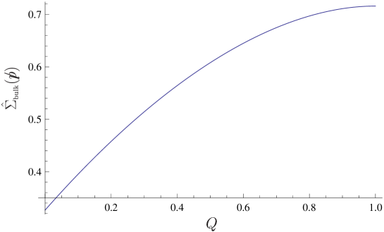
Figure 2: The momentum dependence of $\hat{\Sigma}_{\textrm{\scriptsize bulk}}(p\!\!\!/)$, where $p_{5}=1/L$ and $-10^{3}\leq s\leq 10^{3}$.

The momentum dependence of $\hat{\Sigma}_{\textrm{\scriptsize bulk}}(p\!\!\!/)$ is shown in Figure 2. For modes of the Poisson summation, we take the sum $-10^{3}\leq s\leq 10^{3}$ as the contribution for $|s|>10^{3}$ is much less than ${\cal O}(\%)$. For $Q\sim 0.4$, the linear and logarithmic parts of Eq. (4.12) are comparable. For $0.7\hskip 3.00003pt\raisebox{1.72218pt}{$<$}\raisebox{-3.01385pt}{$\sim$}\hskip 3.00003ptQ\leq 1$, the linear part is dominant. For $Q=1$, i.e., $p\!\!\!/=p_{5}$, the logarithmic part is vanishing. The renormalized bulk self-energy is written as the linear term and the others such as $\hat{\Sigma}_{\textrm{\scriptsize bulk}}\approx 0.7Q+\hat{\Sigma}_{\textrm{\scriptsize bulk}}^{\textrm{\scriptsize nonlinear}}$, where $\hat{\Sigma}_{\textrm{\scriptsize bulk}}|_{Q=1}\simeq 0.7$. For $10^{-5}\leq Q\leq 1$, the bulk self-energy $\hat{\Sigma}_{\textrm{\scriptsize bulk}}$ changes the value by about 50$\%$.

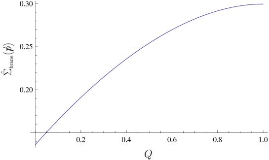
Figure 3: The momentum dependence of $\hat{\Sigma}_{\textrm{\scriptsize brane}}(p\!\!\!/)$, where the value for $p_{5}$ is taken as the same as in Figure 2.

The momentum dependence of $\hat{\Sigma}_{\textrm{\scriptsize brane}}(p\!\!\!/)$ is shown in Figure 3. The behavior is similar to the case of $\hat{\Sigma}_{\textrm{\scriptsize bulk}}$. The brane self-energy is written as the linear term and the others such as $\hat{\Sigma}_{\textrm{\scriptsize brane}}\approx 0.3Q+\hat{\Sigma}_{\textrm{\scriptsize brane}}^{\textrm{\scriptsize nonlinear}}$, where $\hat{\Sigma}_{\textrm{\scriptsize brane}}|_{Q=1}\simeq 0.3$. In addition to each momentum-dependence of the bulk and brane parts, the momentum-dependence of the ratio is important. The ratio of the brane contribution to the bulk contribution is shown in Figure 4.

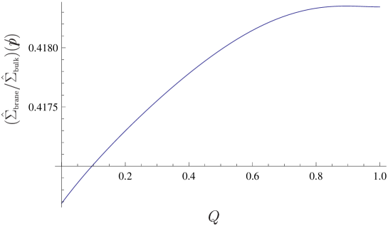
Figure 4: The ratio $(\hat{\Sigma}_{\textrm{\scriptsize brane}}/\hat{\Sigma}_{\textrm{\scriptsize bulk}})(p\!\!\!/)$, where the value for $p_{5}$ is taken as the same as in Figure 2.

For $0.7\hskip 3.00003pt\raisebox{1.72218pt}{$<$}\raisebox{-3.01385pt}{$\sim$}\hskip 3.00003ptQ\leq 1$, the ratio is dominated by the linear term and is approximated as $\hat{\Sigma}_{\textrm{\scriptsize brane}}/\hat{\Sigma}_{\textrm{\scriptsize bulk}}\approx 0.4Q+(\textrm{nonlinear})$, where $0.3/0.7\simeq 0.4$. The nonlinear terms have logarithmic dependence of $Q$ and the change of the value against the momentum-scale is small. For $10^{-5}\leq Q\leq 1$, each of $\hat{\Sigma}_{\textrm{\scriptsize bulk}}$ and $\hat{\Sigma}_{\textrm{\scriptsize brane}}$ changes the value by about 50$\%$. On the other hand, the change of the value for the ratio is less than 0.1$\%$. The momentum insensitivity of the ratio is due to the analogous form seen in $\hat{\Sigma}_{\textrm{\scriptsize bulk}}$ and $\hat{\Sigma}_{\textrm{\scriptsize brane}}$.

From the result for the self-energy, it follows that the ratio of the brane contribution to the bulk contribution is almost constant with respect to the momentum-scale. When $(\delta_{a}-a\delta_{Z})/\delta_{Z}$ is constant, the $\delta_{a}$ is represented in terms of $\delta_{Z}$ as $\delta_{a}=(a+\textrm{constant})\delta_{Z}$. At the leading correction, $a=0$. Then the Lagrangian (2.6) can be represented as

$$\int dy\,\left[\bar{\psi}_{r}(i\partial\!\!\!/)\psi_{r}+\delta_{Z}\left\{\bar{\psi}_{r}(i\partial\!\!\!/)\psi_{r}+0.42\,\bar{\psi}_{rL}(i\partial\!\!\!/)\psi_{rL}\left(\delta(y)+\delta(y-L)\right)\right\}\right],$$ (4.15)

where 0.42 is the value of the ratio for the region in Figure 4. Therefore the relative coefficient between the bulk and brane kinetic terms has been determined without ambiguity.

5 Bulk and brane operators in the distance-rescaling

In this section, we discuss the issue of relevant, irrelevant and marginal operators for bulk and brane terms to identify a general low-energy behavior of quantum corrections in the field-theoretical context.

In Ref. [17], marginal and interacting operators in quantum field theory with extra dimensions were discovered for the Randall-Sundrum spacetime whose metric is given by [18, 19]

$$ds^{2}={1\over z^{2}}\left(\eta_{\mu\nu}dx^{\mu}dx^{\nu}-{1\over k^{2}}dz^{2}\right),$$ (5.1)

where $k$ is the curvature of the five-dimensional anti-de Sitter space. For the four-dimensional rescaling $x^{\prime}=bx$ where $b<1$, the rescaling of $z$ is given by $z^{\prime}=z/b$. The action integral

$$\int d^{4}x{dz\over kz}\left[{1\over z^{3}}\bar{\psi}i\gamma^{\mu}\partial_{\mu}\psi+{1\over 2z^{2}}(\partial_{\mu}\phi)^{2}-{1\over z^{4}}g\bar{\psi}\psi\phi\right],$$ (5.2)

is rescaled into

$$\int d^{4}x^{\prime}{dz^{\prime}\over kz^{\prime}}\left[{1\over{z^{\prime}}^{3}}\bar{\psi}^{\prime}i\gamma^{\mu}\partial^{\prime}_{\mu}\psi^{\prime}+{1\over 2{z^{\prime}}^{2}}(\partial^{\prime}_{\mu}\phi^{\prime})^{2}-{1\over{z^{\prime}}^{4}}g^{\prime}\bar{\psi}^{\prime}\psi^{\prime}\phi^{\prime}\right].$$ (5.3)

Here the field redefinition is given by $\psi^{\prime}=b^{-3}\psi$ and $\phi^{\prime}=b^{-2}\phi$. The coupling constant is given by $g^{\prime}=b^{0}g$ and the corresponding interaction is a marginal operator.

If the spacetime is flat with the rescaling $x^{\prime}=bx$ and $y^{\prime}=by$, the action integral

$$\int d^{4}xdy\left[\bar{\psi}i\gamma^{\mu}\partial_{\mu}\psi+{1\over 2}(\partial_{\mu}\phi)^{2}-g\bar{\psi}\psi\phi\right],$$ (5.4)

is rescaled into

$$\int d^{4}xdy\left[\bar{\psi}^{\prime}i\gamma^{\mu}\partial^{\prime}_{\mu}\psi^{\prime}+{1\over 2}(\partial^{\prime}_{\mu}\phi^{\prime})^{2}-g\bar{\psi}^{\prime}\psi^{\prime}\phi^{\prime}\right].$$ (5.5)

Here the field redefinition is given by $\psi^{\prime}=b^{-2}\psi$ and $\phi^{\prime}=b^{-3/2}\phi$. The coupling constant is given by $g^{\prime}=b^{1/2}g$ and the corresponding operator is an irrelevant operator.

Now we consider the sum of bulk and brane terms. In the flat spacetime, the action integral is given by

$$\int d^{4}xdy\,{\cal L}_{\textrm{\scriptsize bulk}}(\psi,\phi)+\int d^{4}xdy\,{\cal L}_{\textrm{\scriptsize brane}}(\psi,\phi)\delta(y-y_{i}),$$ (5.6)

where $y_{i}$ denote the positions of branes. For the rescaling in the flat spacetime, the action integral is written as

$$\int d^{4}x^{\prime}dy^{\prime}b^{-5}\,{\cal L}_{\textrm{\scriptsize bulk}}(b^{2}\psi^{\prime},b^{3/2}\phi^{\prime})+\int d^{4}x^{\prime}dy^{\prime}b^{-5}\,{\cal L}_{\textrm{\scriptsize brane}}(b^{2}\psi^{\prime},b^{3/2}\phi^{\prime})\delta(y^{\prime}-y^{\prime}_{i})b.$$ (5.7)

The brane terms are multiplied by the factor $b$ compared to the bulk terms. This shows that in the flat spacetime brane kinetic terms are small compared to bulk kinetic terms.

In the Randall-Sundrum spacetime, the action integral corresponding to Eq. (5.6) is given by

$$\int d^{4}xdz\sqrt{\textrm{det}g_{MN}}{\cal L}_{\textrm{\scriptsize bulk}}(\psi,\phi;g_{MN})+\int d^{4}xdz\sqrt{\textrm{det}g_{MN}}{\cal L}_{\textrm{\scriptsize brane}}(\psi,\phi;g_{MN})kz\delta(z-z_{i}).$$ (5.8)

For the rescaling in the Randall-Sundrum spacetime, the action integral is written as

$$\int d^{4}x^{\prime}dz^{\prime}\sqrt{\textrm{det}g^{\prime}_{MN}}b^{-8}{\cal L}_{\textrm{\scriptsize bulk}}(b^{3}\psi^{\prime},b^{2}\phi^{\prime};b^{-2}g^{\prime}_{MN})$$

$$+\int d^{4}x^{\prime}dz^{\prime}\sqrt{\textrm{det}g^{\prime}_{MN}}b^{-8}{\cal L}_{\textrm{\scriptsize brane}}(b^{3}\psi^{\prime},b^{2}\phi^{\prime};b^{-2}g^{\prime}_{MN})kz^{\prime}\delta(z^{\prime}-z^{\prime}_{i}).$$ (5.9)

Because $kz\delta(z-z_{i})=kz^{\prime}\delta(z^{\prime}-z^{\prime}_{i})b^{0}$, the brane kinetic terms are the same order as the bulk kinetic terms.

Our method to determine the momentum-dependence of the bulk and brane contributions has been given in the flat spacetime. In the flat spacetime, the bulk interactions and the brane kinetic terms tend to be irrelevant operators. Thus our explicit analysis may be regarded as the proposal of an idea in a simplified model. On the other hand, in the Randall-Sundrum spacetime, these operators tend to be marginal operators. In the four-dimensional theory, marginal operators are renormalizable terms and low-energy quantum corrections are consistently treated without an additional ultraviolet completion. The idea needs to be examined further in models where the bulk interactions and the brane kinetic terms are marginal operators.

6 Conclusion

We have examined energy-scale dependence of fermion self-energy associated with wave function renormalization in Yukawa theory in flat five dimensions on the $S^{1}/Z_{2}$. At one-loop level, wave function renormalization is needed as in four dimensions. One-loop divergence can be subtracted with only the two renormalization constants $\delta_{Z}$ and $\delta_{a}$ in the bulk and on the branes. We have shown that the bulk and brane parts of the self-energies are uniquely determined with requiring physical conditions. The physical condition is that fields with their physical mass obey usual Feynman propagators. In the present setup, for the right-handed component the bulk part of the self-energy is immediately fixed. The left-handed component determines the other renormalization factor. With this procedure, momentum-scale dependence of the renormalized self-energies has been given. While the loop integral has linear divergence in the cutoff regularization, the renormalized self-energy does not give rise to regularization-scheme dependence. As an explicit equation, the bulk part of the renormalized self-energy is rewritten as

$$\hat{\Sigma}_{\textrm{\scriptsize bulk}}(p\!\!\!/)=\Sigma_{\textrm{\scriptsize bulk}}^{(1)}(p\!\!\!/)-\Sigma_{\textrm{\scriptsize bulk}}^{(1)}(p_{5})-p\!\!\!/\left.\left({d\over dp\!\!\!/}\Sigma_{\textrm{\scriptsize bulk}}^{(1)}(p\!\!\!/)\right)\right|_{p\!\!\!/=p_{5}}.$$ (6.1)

From this equation, it is seen that a constant shift of $\hat{\Sigma}_{\textrm{ \scriptsize bulk}}^{(1)}$ is unphysical. The case of $\hat{\Sigma}_{\textrm{\scriptsize brane}}$ is similar. We have also found that the ratio of the bulk contribution to the brane contribution depends on the momentum scale within less than 0.1$\%$, so that the relative coefficient of bulk and brane kinetic terms can be regarded as approximately constant for the leading quantum effect. The value of the relative coefficient has been estimated as 0.42 for the parameter set given in Section 4. Because the value is not extremely small, it would affect the prediction in phenomenological applications such as collider physics. The quantitative estimation depends on the model.

Analysis beyond the leading level is an open question. In the equation (3.2), divergence for the off-diagonal component with respect to Kaluza-Klein modes has been found. To subtract this divergence, the original action integral would need the corresponding counterterms. As mentioned below Eq. (3.2), linear divergence for the off-diagonal component may correspond to five-dimensional terms in higher-dimensional spacetime. The necessity of new local operators order by order is nothing but non-renormalizability. A possible way to proceed is to show that such local operators are irrelevant. In the present analysis, the relative coefficient of the brane terms to the bulk term is 0.42 which is not negligible. The effects of new operators should be treated carefully. As for regularization-scheme dependence, it needs to be checked whether the scheme independence is kept at higher-loop level. Because the loop-integral is scheme dependent even at the leading level, the momentum-dependent part for any physical quantities might be contributed from such a effect. A viewpoint of this issue is given in the following. When our interest is low energy behavior of physical quantities, details of the scheme-dependent part may not be required. Then we do not need to show that the prediction is exactly scheme independent. Rather, it is sufficient that the scheme-dependence is negligible at low energies. In addition, our analysis has focused on wave function renormalization for two-point functions. To define a physical mass, mass renormalization should be treated appropriately.

Finally we emphasize that the physical conditions given here are applicable to remove ambiguity in various orbifold models. We have also shown that both of the bulk and brane kinetic terms are marginal operators in the Randall-Sundrum spacetime. It would be worthwhile to identify the momentum-dependence of bulk and brane contributions in such models.

Acknowledgments

This work is supported by Scientific Grants from the Ministry of Education and Science, Grant No. 20244028.

Appendix A Yukawa theory on an orbifold

We consider a five-dimensional Yukawa theory on the orbifold $S^{1}/Z_{2}$. The bulk spacetime is flat with the metric $\eta^{MN}=\textrm{diag}(1,-1,-1,-1,-1)$. The action integral for the Dirac fermion $\psi(x,y)$ and the real scalar field $\phi(x,y)$ is

$$S=\int d^{4}x\,\cdot{1\over 2}\int_{-L}^{L}dy\,\left[\bar{\psi}(i\gamma^{\mu}\partial_{\mu}+i\gamma^{5}\partial_{5})\psi+{1\over 2}(\partial_{\mu}\phi)^{2}-{1\over 2}(\partial_{5}\phi)^{2}-g\bar{\psi}\psi\phi\right].$$ (A.1)

Greek indices $\mu$ run over 0,1,2,3 and fifth index is denoted as $y$. The gamma matrices are

$$\gamma^{\mu}=\left(\begin{array}[]{cc}&\sigma^{\mu}\\ \bar{\sigma}^{\mu}&\\ \end{array}\right),\qquad-i\gamma^{5}=\left(\begin{array}[]{cc}-{\bf 1}_{2}&\\ &{\bf 1}_{2}\\ \end{array}\right)=i\gamma_{5},$$ (A.6)

where $\sigma^{\mu}=({\bf 1}_{2},\sigma^{i})$ and $\bar{\sigma}^{\mu}=(-{\bf 1}_{2},\sigma^{i})$ with the Pauli matrices. Dirac conjugate is given by $\bar{\psi}=\psi^{\dagger}\gamma^{0}$. The fields have period $2L$ with respect to the extra dimension. The orbifold boundary conditions for the fields are chosen as

$$\psi(x,-y) \!\!\!=\!\!\! i\gamma^{5}\psi(x,y),\qquad\psi(x,L-y)=i\gamma^{5}\psi(x,L+y),$$ (A.7)

$$\phi(x,-y) \!\!\!=\!\!\! -\phi(x,y),\qquad\phi(x,L-y)=-\phi(x,L+y),$$ (A.8)

for the extra-dimensional fundamental region $0\leq y\leq L$. With this boundary conditions, the fermion has mode expansion as

$$\psi_{L}(x,y) \!\!\!=\!\!\! {1\over\sqrt{L}}\,\chi_{L}(x)+\sum_{n=1}^{\infty}\sqrt{2\over L}\,\psi_{Ln}(x)\cos\left(m_{n}y\right),$$ (A.9)

$$\psi_{R}(x,y) \!\!\!=\!\!\! \sum_{n=1}^{\infty}\sqrt{2\over L}\,\psi_{Rn}(x)\sin\left(m_{n}y\right).$$ (A.10)

with $m_{n}=n\pi/L$. The projection matrices are given by $P_{L}=\left[{\bf 1}_{2}-(-i\gamma^{5})\right]/2=\textrm{diag}(1,1,0,0)$ and $P_{R}=\left[{\bf 1}_{2}+(-i\gamma^{5})\right]/2=\textrm{diag}(0,0,1,1)$. The mode expansion of the scalar $\phi(x,y)$ is similar to Eq. (A.10). The mode functions and the above trigonometric functions are periodic for $y\to y+2L$. From the properties of orthogonality and completeness, quadratic terms in the action integral (A.1) are

$${1\over 2}\int_{-L}^{L}dy\,\left[\bar{\psi}(i\gamma^{\mu}\partial_{\mu}+i\gamma^{5}\partial_{5})\psi+{1\over 2}(\partial_{\mu}\phi)^{2}-{1\over 2}(\partial_{5}\phi)^{2}\right]$$ (A.11)

$$\!\!\!=\!\!\! \bar{\chi}_{L}(i\gamma^{\mu}\partial_{\mu})\chi_{L}+\sum_{n=1}^{\infty}\left[\bar{\psi}_{n}(i\gamma^{\mu}\partial_{\mu}-m_{n})\psi_{n}+{1\over 2}(\partial_{\mu}\phi_{n})^{2}+{1\over 2}(m_{n}\phi_{n})^{2}\right].$$

where $\psi_{n}$ is composed of $\psi_{Ln}$ and $\psi_{Rn}$ as in the left- and right-handed projections for $\psi$. The equation (A.11) is diagonal with respect to Kaluza-Klein modes. The Yukawa interaction is written in terms of four-dimensional modes as

$${1\over 2}\int_{-L}^{L}dy\,(-g)\bar{\psi}\psi\phi \!\!\!=\!\!\! \sum_{n=1}^{\infty}{(-g)\over\sqrt{L}}\left[\bar{\chi}_{L}\psi_{Rn}\phi_{n}+\bar{\psi}_{Rn}\chi_{L}\phi_{n}\right]$$ (A.12)

$$+\sum_{n=1}^{\infty}\sum_{\ell=1}^{\infty}\sum_{k=1}^{\infty}{(-g)\over\sqrt{2L}}\,\bar{\psi}_{Ln}\psi_{R\ell}\phi_{k}\left\{\delta_{k+n,\ell}+\delta_{\ell+n,k}-\delta_{k+\ell,n}\right\}$$

$$+\sum_{n=1}^{\infty}\sum_{\ell=1}^{\infty}\sum_{k=1}^{\infty}{(-g)\over\sqrt{2L}}\,\bar{\psi}_{Rn}\psi_{L\ell}\phi_{k}\left\{\delta_{n+\ell,k}+\delta_{k+\ell,n}-\delta_{n+k,\ell}\right\}.$$

The Yukawa interaction involves the exchange between Kaluza-Klein modes. Originally the kinetic terms are set only in the bulk. In the next section, it will be shown that divergence corresponding to brane kinetic terms is radiatively generated.

Appendix B Method of loop calculations

As in four dimensions, wave function renormalization is expected to appear for the fermion at the one-loop level. The appearance of divergence on the branes in a similar setup is shown in Ref. [1]. For the calculation of quantum loop corrections, the steps we perform contain the Kaluza-Klein mode expansion, the summation of diagrams, the replacement of fractions with a formula for the Gamma function and the representation with the Poisson summation for the summation of the Kaluza-Klein modes. In this appendix, we give explicit equations at each step in the method to calculate self energy for the action integral (A.1). The method will be used further in Section 3.

The first diagram is the self-energy for the left-handed fermion zero mode. The external lines are the left-handed zero mode $\chi$ and the internal lines are $\phi_{n}$ and $\psi_{Rn}$. The internal lines are summed with respect to all $n$. The diagram is shown in Fig. 5.

Figure 5: Self-energy diagram for the left-handed zero mode.

The self-energy up to the propagators for the external lines is

$${g^{2}\over L}\sum_{n=1}^{\infty}\int{d^{4}k\over(2\pi)^{4}}{k\!\!\!/+m_{n}\over k^{2}-m_{n}^{2}}P_{L}{1\over(p-k)^{2}-m_{n}^{2}}={g^{2}\over L}\sum_{n=1}^{\infty}\int_{0}^{1}dx\int{d^{4}\ell\over(2\pi)^{4}}{xp\!\!\!/+m_{n}\over\left[\ell^{2}-\Delta_{n}\right]^{2}}P_{L},$$ (B.1)

with a Feynman parameter $x$. Here $\ell=k-xp$ and $\Delta_{n}=-x(1-x)p^{2}+m_{n}^{2}$. We will focus on $p\!\!\!/$ terms, i.e., the terms for the wave function renormalization, neglecting $m_{n}$ in the numerator. Then the integrand is symmetric under $n\leftrightarrow-n$. The $p\!\!\!/$ term in Eq. (B.1) is rewritten as

$${g^{2}\over 2L}\sum_{n=-\infty}^{\infty}\int_{0}^{1}dx\int{d^{4}\ell\over(2\pi)^{4}}{x(ip\!\!\!/)\over\left[\ell_{E}^{2}+\Delta_{n}\right]^{2}}P_{L}-{g^{2}\over 2L}\int_{0}^{1}dx\int{d^{4}\ell_{E}\over(2\pi)^{4}}{x(ip\!\!\!/)\over\left[\ell_{E}^{2}+\Delta_{0}\right]^{2}}P_{L},$$ (B.2)

with the Wick rotation $\ell^{0}=i\ell_{E}^{0}$ and $\ell^{i}=\ell^{i}_{E}$. With use of symmetry under $n\leftrightarrow-n$, the sum in the first term has been taken for $-\infty\leq n\leq\infty$ which is more convenient than treating the sum for $1\leq n\leq\infty$. For this infinite sum, a formula for the Poisson summation will be employed. The second term in Eq. (B.2) is independent of internal mode $n$.

Let us calculate the sum part $\sum_{n=-\infty}^{\infty}$. The first step is to rewrite the fraction using the integral representation of the Gamma function as

$${1\over\left[\ell_{E}^{2}+\Delta_{n}\right]^{2}}={1\over\Gamma(2)}\int_{0}^{\infty}dt\,te^{-(\ell_{E}^{2}+\Delta_{n})t}=\int_{0}^{\infty}dt\,te^{-(\ell_{E}^{2}-x(1-x)p^{2}+{n^{2}\pi^{2}\over L^{2}})t}.$$ (B.3)

The second step is to change the mode index with the Poisson summation,

$$\sum_{n=-\infty}^{\infty}e^{-n^{2}{\pi^{2}t\over L^{2}}}={L\over\sqrt{\pi t}}\sum_{n_{p}=-\infty}^{\infty}e^{-n_{p}^{2}{L^{2}\over t}}.$$ (B.4)

Then the sum part, the first term in Eq. (B.2), is written as

$${g^{2}\over 2^{5}\pi^{5\over 2}}\int_{0}^{1}dx\,x(ip\!\!\!/)\sum_{n_{p}=-\infty}^{\infty}\int_{0}^{\infty}dt\,t^{-{3\over 2}}e^{x(1-x)p^{2}t-{n_{p}^{2}L^{2}\over t}}\,P_{L},$$ (B.5)

where the Gaussian integral for $\ell_{E}$ have been employed. The next step is to evaluate each part for $n_{p}=0$ and $n_{p}\neq 0$. The $n_{p}=0$ part includes divergence for $t\to 0$. The divergence of the $t$ integral is evaluated as

$$\int_{0}^{\infty}dt\,t^{-{3\over 2}}(1+x(1-x)p^{2}t+\cdots)=\left[-2t^{-{1\over 2}}+\cdots\right]_{t=\Lambda^{-2}}^{t=\infty}=2\Lambda+\textrm{finite},$$ (B.6)

at the cutoff regularization. This momentum integral depends on the regularization scheme. The scheme-independence of the renormalized quantity will be shown in Section 4. The divergence of the $n_{p}=0$ part is

$${g^{2}\over 2^{5}\pi^{5\over 2}}\int_{0}^{1}dx\,x(ip\!\!\!/)\cdot 2\Lambda\,P_{L}={g^{2}\over 2L(4\pi)^{2}}{\Lambda L\over\sqrt{\pi}}(ip\!\!\!/)P_{L}.$$ (B.7)

From the mass dimensions for the fields and coupling $[\psi]=[\textrm{mass}]^{2}$, $[\phi]=[\textrm{mass}]^{3/2}$, $[g]=[\textrm{mass}]^{-{1/2}}$, the bulk divergence for the wave function is expected to have the coefficient $g^{2}\Lambda$ where $[g^{2}\Lambda]=[\textrm{mass}]^{0}$ and it is consistent with Eq. (B.7). The $n_{p}\neq 0$ part is

$${g^{2}\over 2^{3}\pi^{5\over 2}}\int_{0}^{1}dx\,x(ip\!\!\!/)\sum_{n_{p}=1}^{\infty}{\sqrt{\pi}\over 2n_{p}L}e^{-2n_{p}L{\sqrt{-x(1-x)p^{2}}}}P_{L},$$ (B.8)

where the integral for $t$ has been performed with help of expressions for Bessel function $K_{\nu}$. If a function $F(x)$ is symmetric under the exchange $x\leftrightarrow 1-x$, $F(x)=F(1-x)$, then $\int_{0}^{1}dx\,xF(x)=\int_{0}^{1}dx\,(1-x)F(x)=(1/2)\int_{0}^{1}dx\,F(x)$. The equation (B.8) becomes

$$-{g^{2}\over 2L(4\pi)^{2}}\int_{0}^{1}dx\,(ip\!\!\!/)\log\left[1-e^{-2L\sqrt{-x(1-x)p^{2}}}\right]\cdot P_{L},$$ (B.9)

where the sum for $n_{p}$ has been performed with the Taylor series expansion $\log(1-X)=-\sum_{s=1}^{\infty}{X^{s}/s}$.

Now we move on to the second line in Eq. (B.2),

$$(\Delta_{0}~{}\textrm{part})=-{g^{2}\over 2L}\int_{0}^{1}dx\int{d^{4}\ell_{E}\over(2\pi)^{4}}{x(ip\!\!\!/)\over\left[\ell_{E}^{2}+\Delta_{0}\right]^{2}}P_{L},$$ (B.10)

where $\Delta_{0}=-x(1-x)p^{2}$. This is a usual four-dimensional integral. For the cutoff regularization, Eq. (B.10) is given by

$$-{g^{2}\over 2L(4\pi)^{2}}(ip\!\!\!/)\left(\log(\Lambda L)-{1\over 2}\log(-p^{2}L^{2})+1\right)\cdot P_{L}.$$ (B.11)

This divergence is expected from the dimensional counting $[g^{2}]=[\textrm{mass}]^{-1}$ and $[1/L]=[\textrm{mass}]$. For the self-energy with the field $\chi$ in the external lines, we have found linear divergence in the summation part $\sum_{n=-\infty}^{\infty}$ and logarithmic divergence in the non-summation part.

The self-energy with the field $\psi_{L}$ in the external lines is analogous. Here there are various Kaluza-Klein modes to contribute. The internal lines are composed of $\phi$ and $\psi_{R}$. The Kaluza-Klein modes for the external and internal lines are labeled as shown in Figure 1. The momentum flow is the same as in Figure 5. With the same procedure as in obtaining Eq. (B.2) from Eq. (B.1) for the diagram in Figure 5, the part $p\!\!\!/$ in the sum of the diagrams (a), (b) and (c) in Figure 1 is obtained as

$$(\textrm{(a)}+\textrm{(b)}+\textrm{(c)})|_{p\!\!\!/} \!\!\!=\!\!\! {g^{2}\over 2L}\sum_{s=-\infty}^{\infty}\int_{0}^{1}dx\int{d^{4}\ell\over(2\pi)^{4}}\,{xp\!\!\!/\over\left[\ell^{2}-\Delta_{s+}\right]^{2}}P_{L}$$ (B.12)

$$-{g^{2}\over 2L}\int_{0}^{1}dx\int{d^{4}\ell\over(2\pi)^{4}}\,{xp\!\!\!/\over\left[\ell^{2}-\Delta_{0+}\right]^{2}}P_{L}$$

$$-{g^{2}\over 2L}\int_{0}^{1}dx\int{d^{4}\ell\over(2\pi)^{4}}\,{xp\!\!\!/\over\left[\ell^{2}-\Delta_{n+}\right]^{2}}P_{L}.$$

Here $\Delta_{s+}=-x(1-x)p^{2}+(s+(1-x)n)^{2}\pi^{2}/L^{2}+x(1-x)n^{2}\pi^{2}/L^{2}$. The other $\Delta_{0+}$ and $\Delta_{n+}$ are obtained from $\Delta_{s}+$ as $\Delta_{0+}=\Delta_{s+}|_{s=0}$ and $\Delta_{n+}=\Delta_{s+}|_{s=n}$. The divergent part is given by

$$((\textrm{a})+(\textrm{b})+(\textrm{c}))|_{\textrm{\scriptsize div}} \!\!\!=\!\!\! {g^{2}\over 2L(4\pi)^{2}}(ip\!\!\!/)\left[{\Lambda L\over\sqrt{\pi}}-\log(\Lambda^{2}L^{2})\right]\cdot P_{L}.$$ (B.13)

For the diagrams (d), (e), (f) and (g) in Figure 1, the external lines have $n$ and $n+2s$. The modes $n$ and $s$ in the internal lines are fixed for given external lines. These correspond to the non-sum part in Eq. (B.2). These diagrams satisfy $\textrm{(g)}=\textrm{(d)}$ and $\textrm{(f)}=\textrm{(e)}$. The divergent part is

$$(\textrm{d})|_{\textrm{\scriptsize div}}=(\textrm{g})|_{\textrm{\scriptsize div}} \!\!\!=\!\!\! -{g^{2}\over 4L(4\pi)^{2}}(ip\!\!\!/)\log(\Lambda^{2}L^{2})\cdot P_{L}$$ (B.14)

$$\!\!\!=\!\!\! (\textrm{f})|_{\textrm{\scriptsize div}}=(\textrm{e})|_{\textrm{\scriptsize div}}.$$

The self-energy with the fields $\chi$ and $\psi_{L}$ in the external lines is similarly calculated.

The other diagrams are the ones that have the right-handed field $\psi_{R}$ in the external lines. Similarly to diagrams with $\psi_{L}$ in an external line, the Kaluza-Klein modes are labeled. For (a), (b), $\cdots$, (g), there are the corresponding diagrams (a^′), (b^′), $\cdots$, (g^′). The amplitudes (a^′), (b^′), (c^′), (d^′) and (g^′) are given by (a), (b), (c), (d) and (g) with $P_{L}$ replaced by $P_{R}$. The amplitudes (e^′) and (f^′) are given by (e) and (f) with $P_{L}$ replaced by $P_{R}$ and with the change of the overall sign. In addition to these diagrams, there is a diagram with $\psi_{R}$ in the external lines and with $\chi$ and $\phi$ in the internal lines. This contributes to the divergent part as

$${g^{2}\over 2L(4\pi)^{2}}(ip\!\!\!/)\log(\Lambda^{2}L^{2})\cdot P_{R}.$$ (B.15)

The equation (B.15) and the last term in Eq. (B.13) with the replacement $P_{L}$ by $P_{R}$ cancel each other. The contributions (d^′) and (e^′) cancel each other and (f^′) and (g^′) cancel each other. In summary for the right-handed external lines, the remaining divergence is

$${g^{2}\over 2L(4\pi)^{2}}(ip\!\!\!/){\Lambda L\over\sqrt{\pi}}\cdot P_{R}.$$ (B.16)

The logarithmic divergence for the external $\psi_{R}$ is canceled out.

The final step in the loop calculation is to identify Lagrangian terms corresponding to the divergence. For all the divergences (B.13), (B.14) and (B.16), the Lagrangian terms are given by

$${(-i)g^{2}\over 2L(4\pi)^{2}}{\Lambda L\over\sqrt{\pi}}\left(\bar{\chi}_{L}(ip\!\!\!/)\chi_{L}+\sum_{n}\bar{\psi}_{n}(ip\!\!\!/)\psi_{n}\right)$$

$$-{(-i)g^{2}\over 2L(4\pi)^{2}}\log(\Lambda L)\bigg{\{}\bar{\chi}_{L}(ip\!\!\!/)\chi_{L}+2\sum_{n}\bar{\psi}_{n,L}(ip\!\!\!/)\psi_{n,L}$$

$$+2\sum_{n}\sum_{s}\left(\bar{\psi}_{n,L}(ip\!\!\!/)\psi_{n+2s,L}+\bar{\psi}_{n+2s,L}(ip\!\!\!/)\psi_{n,L}\right)$$

$$+\sqrt{2}\sum_{n}\left(\bar{\chi}_{L}(ip\!\!\!/)\psi_{2n,L}+\bar{\psi}_{2n,L}(ip\!\!\!/)\chi_{L}\right)\bigg{\}}.$$ (B.17)

From this equation, the Lagrangian terms with four-derivative are written in terms of the five-dimensional field as

$${g^{2}\over 2L(4\pi)^{2}}\cdot{1\over 2}\lim_{\epsilon\to 0}\int_{-L+\epsilon}^{L+\epsilon}dy\left[{\Lambda L\over\sqrt{\pi}}\,\bar{\psi}(i\partial\!\!\!/)\psi-\log(\Lambda L)\,\bar{\psi}_{L}(i\partial\!\!\!/)\psi_{L}\left(\delta(y)+\delta(y-L)\right)\right],$$ (B.18)

where $\lim_{\epsilon\to 0}\int_{-L+\epsilon}^{L+\epsilon}dy\,G(y)\left[\delta(y)+\delta(y-L)\right]=G(0)+G(L)$. The divergence in the brane terms for one-loop wave function occurs in the equal size at $y=0$ and at $y=L$, in agreement with Ref. [1]. For the boundary condition (A.7), the right-handed component $\psi_{R}$ does not have the brane term. In the equation (B.18), the brane divergence includes non-diagonal components with respect to Kaluza-Klein modes and the bulk divergence is diagonal.

Appendix C Mode functions

According to the approach given in Ref. [9], we derive $f_{n}$ and $g_{n}$. The fermion mode functions appearing in the context, $f_{n}$ and $g_{n}$, are $f_{n\,\textrm{\scriptsize III}}$ and $g_{n\,\textrm{\scriptsize III}}$ given in this appendix.

From the equations of motion (2.8) and (2.9) and Eq. (2.10), the mode functions obey

$$\partial_{y}f_{n} \!\!\!=\!\!\! -m_{n}g_{n},$$ (C.1)

$$\partial_{y}g_{n} \!\!\!=\!\!\! m_{n}\left(1+a\,\left(\delta(y)+\delta(y-L)\right)\right)f_{n},$$ (C.2)

for $n\neq 1$. From these equations, the second-order differential equation for $f_{n}$ is obtained as

$$\left(\partial_{y}^{2}+m_{n}^{2}+a\,m_{n}^{2}\left(\delta(y)+\delta(y-L)\right)\right)f_{n}=0.$$ (C.3)

Unless confusion arises, we will omit the subscript for the Kaluza-Klein mode number $n$ for $f_{n}$. The equation (C.3) includes two delta functions. It is convenient to write the function by defining separate regions in a period $2L$. The regions can be classified as shown in Figure 6.

Figure 6: Regions. Allows depict $\delta$ functions

In each region, the function $f$ where is written as

$$f_{\textrm{\scriptsize I}}(y) \!\!\!=\!\!\! Ae^{imy}+Be^{-imy},$$ (C.4)

$$f_{\textrm{\scriptsize II}}(y) \!\!\!=\!\!\! Ce^{imy}+De^{-imy},$$ (C.5)

$$f_{\textrm{\scriptsize III}}(y) \!\!\!=\!\!\! Ee^{imy}+Fe^{-imy},$$ (C.6)

$$f_{\textrm{\scriptsize IV}}(y) \!\!\!=\!\!\! Ge^{imy}+He^{-imy},$$ (C.7)

where $A,B,C,D,E,F,G,H$ are determined by 8 conditions. They are periodicity between the regions I and III and between the regions II and IV, continuity at $y=-L,0,L$, matching of the first derivative at $y=-L,0,L$ and the normalization. Among the above 9 conditions, one condition is automatically satisfied if the other conditions are satisfied.

Now we fix these constants. The periodicity requires

$$Ae^{im(y-2L)}+Be^{-m(y-2L)}=Ee^{imy}+Fe^{-imy},$$ (C.8)

$$Ce^{im(y-2L)}+De^{-m(y-2L)}=Ge^{imy}+He^{-imy}.$$ (C.9)

The continuity requires

$$Ae^{-imL}+Be^{imL}=Ce^{-imL}+De^{imL},$$ (C.10)

$$C+D=E+F,$$ (C.11)

$$Ee^{imL}+Fe^{-imL}=Ge^{imL}+He^{-imL},$$ (C.12)

at $y=-L,0,L$, respectively. The matching of first derivative requires

$$\left[\partial_{y}f_{n}\right]_{\textrm{\scriptsize I}}^{\textrm{\scriptsize II}}+a\,m_{n}^{2}f_{n\textrm{\scriptsize I}}|_{y=-L}=0,$$ (C.13)

$$\left[\partial_{y}f_{n}\right]_{\textrm{\scriptsize II}}^{\textrm{\scriptsize III}}+am_{n}^{2}f_{n\textrm{\scriptsize II}}|_{y=0}=0,$$ (C.14)

$$\left[\partial_{y}f_{n}\right]_{\textrm{\scriptsize III}}^{\textrm{\scriptsize IV}}+am_{n}^{2}f_{n\textrm{\scriptsize III}}|_{y=L}=0,$$ (C.15)

at $y=-L,0,L$, respectively. Here $f_{n\textrm{\scriptsize I}}$ in the second term in Eq. (C.13) can be replaced by $f_{n\textrm{\scriptsize II}}$ because of the continuity (C.10). The equations (C.14) and (C.15) are understood similarly. In summary, the conditions up to normalization are

$$Ae^{im(y-2L)}+Be^{-im(y-2L)}=Ee^{imy}+Fe^{-imy},\qquad(\textrm{for}~{}0_{+}\leq y\leq L_{-}),$$ (C.16)

$$Ce^{im(y-2L)}+De^{-im(y-2L)}=Ge^{imy}+He^{-imy},\qquad(\textrm{for}~{}L_{+}\leq y\leq 2L_{-}),$$ (C.17)

$$Ae^{-imL}+Be^{imL}=Ce^{-imL}+De^{imL},$$ (C.18)

$$C+D=E+F,$$ (C.19)

$$Ee^{imL}+Fe^{-imL}=Ge^{imL}+He^{-imL},$$ (C.20)

$$Ce^{-imL}-De^{imL}-A(1+iam)e^{-imL}+B(1-iam)e^{imL}=0,$$ (C.21)

$$E-F-C(1+iam)+D(1-iam)=0,$$ (C.22)

$$Ge^{imL}-He^{-imL}-E(1+iam)e^{imL}+F(1-iam)e^{-imL}=0,$$ (C.23)

where $0_{+}=\lim_{\epsilon\to 0}0+\epsilon$ and $L_{\mp}=\lim_{\epsilon\to 0}L\mp\epsilon$. Using the first three equations (C.16), (C.17) and (C.18), the fifth condition (C.20) is automatically satisfied. Hence, the above 7 conditions and the normalization fix the 8 constants $A,B,\cdots,H$. Up to the normalization, the solution of the mode function $f$ is given by

$$f_{\textrm{\scriptsize I}}(y) \!\!\!=\!\!\! A(e^{imy}+w^{3}e^{-imy}),$$ (C.24)

$$f_{\textrm{\scriptsize II}}(y) \!\!\!=\!\!\! A(we^{imy}+w^{2}e^{-imy}),$$ (C.25)

$$f_{\textrm{\scriptsize III}}(y) \!\!\!=\!\!\! A(w^{2}e^{imy}+we^{-imy}),$$ (C.26)

$$f_{\textrm{\scriptsize IV}}(y) \!\!\!=\!\!\! A(w^{3}e^{imy}+e^{-imy}),$$ (C.27)

with the mass quantization condition

$$-\tan mL={am\over 1-\left({am\over 2}\right)^{2}},$$ (C.28)

which is also written as $e^{-2imL}=(2+iam)^{2}/(2-iam)^{2}$. Here $w_{n}\equiv(2+iam_{n})/(2-iam_{n})$.

The orthogonality of the mode function can be found as follows. The mode function satisfies the second-order differential equation (C.3). From this equation, the following equation is derived:

$$0 \!\!\!=\!\!\! {1\over 2}\lim_{\epsilon\to 0}\int_{-L+\epsilon}^{L+\epsilon}dy\,\bigg{\{}f_{m}\left(\partial_{y}^{2}+m_{n}^{2}+am_{n}^{2}\left(\delta(y)+\delta(y-L)\right)\right)f_{n}$$ (C.29)

$$-f_{n}\left(\partial_{y}^{2}+m_{m}^{2}+am_{m}^{2}\left(\delta(y)+\delta(y-L)\right)\right)f_{m}\bigg{\}}.$$

It is found that the mode function satisfies

$$\lim_{\epsilon\to 0}(f_{m}\partial_{y}f_{n})_{\textrm{\scriptsize IV},L+\epsilon} \!\!\!=\!\!\! A_{m}A_{n}(w_{m}+1)^{-im_{m}L}(w_{n}-1)im_{n}e^{-im_{n}L}$$ (C.30)

$$\!\!\!=\!\!\! \lim_{\epsilon\to 0}(f_{m}\partial_{y}f_{n})_{\textrm{\scriptsize II},-L+\epsilon},$$

and

$$\int_{-L}^{0}dy\,f_{\textrm{\scriptsize II}n}(y)f_{\textrm{\scriptsize II}m}(y)=\int_{L}^{0}d(-y)\,f_{\textrm{\scriptsize II}n}(-y)f_{\textrm{\scriptsize II}m}(-y)=\int_{0}^{L}dy\,f_{\textrm{\scriptsize III}n}(y)f_{\textrm{\scriptsize III}m}(y).$$ (C.31)

Using these equations, Eq. (C.29) becomes

$$0=(m_{n}^{2}-m_{m}^{2})\left\{\int_{0}^{L}dy\,f_{n}(y)f_{m}(y)+{a\over 2}\left(f_{n}(0)f_{m}(0)+f_{n}(L)f_{m}(L)\right)\right\},$$ (C.32)

where $\lim_{\epsilon\to 0}\int_{L}^{L+\epsilon}dy\,(\textrm{smooth function})=0$. Therefore the orthogonality is given in Eq. (2.11). Here $A$ is normalized as

$$2A^{2}w^{3}\left(L+{4a\over 4+a^{2}m^{2}}\right)=1.$$ (C.33)

The completeness corresponds to

$$\sum_{m}f_{m}(y)f_{m}(y^{\prime})=2\delta(y-y^{\prime})-a\,\left(\delta(y)+\delta(y-L)\right)\sum_{m}f_{m}(y)f_{m}(y^{\prime}).$$ (C.34)

The mode function $g(y)$ is derived from the relation $g=-(1/m)\partial_{y}f$. They are

$$g_{\textrm{\scriptsize I}}(y) \!\!\!=\!\!\! -Ai(e^{imy}-w^{3}e^{-imy}),$$ (C.35)

$$g_{\textrm{\scriptsize II}}(y) \!\!\!=\!\!\! -Ai(we^{imy}-w^{2}e^{-imy}),$$ (C.36)

$$g_{\textrm{\scriptsize III}}(y) \!\!\!=\!\!\! -Ai(w^{2}e^{imy}-we^{-imy}),$$ (C.37)

$$g_{\textrm{\scriptsize IV}}(y) \!\!\!=\!\!\! -Ai(w^{3}e^{imy}-e^{-imy}).$$ (C.38)

The function $g$ has the orthogonality given in Eq. (2.12). Here $+$ in $\pm$ has been adopted as $w_{n}=e^{-imy}$ in $\pm e^{-imy}$. In the limit $a=0$, these mode functions reduce to the mode functions in Eqs. (A.9) and (A.10).

References

- [1] H. Georgi, A. K. Grant and G. Hailu, Phys. Lett. B 506, 207 (2001) [arXiv:hep-ph/0012379].
- [2] L. J. Hall and Y. Nomura, Phys. Rev. D 64, 055003 (2001) [arXiv:hep-ph/0103125].
- [3] G. von Gersdorff, N. Irges and M. Quiros, Nucl. Phys. B 635, 127 (2002) [arXiv:hep-th/0204223].
- [4] H. C. Cheng, K. T. Matchev and M. Schmaltz, Phys. Rev. D 66, 036005 (2002) [arXiv:hep-ph/0204342].
- [5] M. S. Carena, T. M. P. Tait and C. E. M. Wagner, Acta Phys. Polon. B 33, 2355 (2002) [arXiv:hep-ph/0207056].
- [6] F. del Aguila, M. Perez-Victoria and J. Santiago, JHEP 0302, 051 (2003) [arXiv:hep-th/0302023].
- [7] D. M. Ghilencea, JHEP 0503, 009 (2005) [arXiv:hep-ph/0409214].
- [8] A. Muck, L. Nilse, A. Pilaftsis and R. Ruckl, Phys. Rev. D 71, 066004 (2005) [arXiv:hep-ph/0411258].
- [9] G. R. Dvali, G. Gabadadze, M. Kolanovic and F. Nitti, Phys. Rev. D 64, 084004 (2001) [arXiv:hep-ph/0102216].
- [10] M. Chaichian and A. Kobakhidze, arXiv:hep-ph/0208129.
- [11] F. del Aguila, M. Perez-Victoria and J. Santiago, Acta Phys. Polon. B 34, 5511 (2003) [arXiv:hep-ph/0310353].
- [12] F. del Aguila, M. Perez-Victoria and J. Santiago, Eur. Phys. J. C 33, S773 (2004) [arXiv:hep-ph/0310352].
- [13] M. S. Carena, A. Delgado, E. Ponton, T. M. P. Tait and C. E. M. Wagner, Phys. Rev. D 71, 015010 (2005) [arXiv:hep-ph/0410344].
- [14] C. Csaki, J. Hubisz and P. Meade, arXiv:hep-ph/0510275.
- [15] D. M. Ghilencea, H. M. Lee and K. Schmidt-Hoberg, JHEP 0608, 009 (2006) [arXiv:hep-ph/0604215].
- [16] N. Uekusa, Nucl. Phys. B 827, 311 (2010) [arXiv:0909.0825 [hep-ph]].
- [17] N. Uekusa, arXiv:1008.0487 [hep-ph].
- [18] L. Randall and R. Sundrum, Phys. Rev. Lett. 83, 3370 (1999) [arXiv:hep-ph/9905221].
- [19] L. Randall and R. Sundrum, Phys. Rev. Lett. 83, 4690 (1999) [arXiv:hep-th/9906064].