Searching for gravitational waves emitted by binaries with spinning components

Abstract

In this thesis we consider the data analysis problem of detecting gravitational waves emitted by inspiraling binary systems. Detection of gravitational waves will open a new window on the Universe enabling direct detection of systems such as binary black holes for the first time. In the first Chapter we show how gravitational waves are derived from Einstein’s General theory of Relativity and discuss the emission of gravitational waves from inspiraling binaries and how this radiation may be detected using laser interferometers. Around two thirds of stars inhabit binary systems. As they orbit each other they will emit both energy and angular momentum in the form of gravitational waves which will inevitably lead to their inspiral and eventual merger. To date, searches for gravitational waves emitted during the inspiral of binary systems have concentrated on systems with non-spinning components. In Chapter 2 we detail the first dedicated search for binaries consisting of spinning stellar mass compact objects. We analysed 788 hours of data collected during the third science run (S3) of the LIGO detectors, no detection of gravitational waves was made and we set an upper limit on the rate of coalescences of stellar mass binaries. The inspiral of stellar mass compact objects into super massive black holes will radiate gravitational waves at frequencies detectable by the planned space-based LISA mission. In Chapter 3 we describe the development and testing of a computationally cheap method to detect the loudest few extreme mass ratio inspiral events that LISA will be sensitive to.

Conventions

Masses are quoted in units of solar mass

$$1\,M_{\odot}=1.98892\times 10^{30}\mbox{kg}$$ (1)

Distances are quoted in units of parsecs

$$1\,\mbox{pc}=3.0856775807\times 10^{16}\mbox{m}$$ (2)

The values used here are the same as those used within the LIGO Scientific Collaboration Algorithm Library (LAL) and are taken from Barnett et al. (1996) [21].

In mathematical formulae bold face will denote a vector, e.g. ${\bf S}_{1}$ and overhats to represent unit vectors, e.g. $\bf{\bf\hat{S}}_{1}$.

All angles will be in radians.

In general Greek indices sum over ($0\dots 3$) and Latin indices sum over ($1\dots 3$).

We will denote the inner product as $\left<g,h\right>$ and will use $||g||$ to mean $\left<g,g\right>$.

There are two possible sign conventions used to define the Fourier transform. Following the conventions used in LAL we shall define the Fourier transform $\tilde{g}(t)$ of a time domain function $g(t)$ by

$$\tilde{g}(f)=\int_{-\infty}^{\infty}g(t)e^{-2\pi ift}dt$$ (3)

and the inverse Fourier transform by

$$g(t)=\int_{-\infty}^{\infty}\tilde{g}(f)e^{2\pi ift}df.$$ (4)

Note that in some of the literature referenced in this thesis the other convention is used.

We will use geometric units (i.e., $c=G=1$) throughout unless we specify otherwise.

Chapter 1 Introduction

Gravitational waves are an inescapable consequence of any theory of gravity that is consistent with Einstein’s Special Theory of Relativity (1905), in particular its condition that information cannot propagate at speeds greater than the speed of light in vacuum, c. Following Einstein’s General Theory of Relativity (1915) we identify gravity as a curvature of spacetime and gravitational waves to be caused by the acceleration of matter. Gravitational waves carry away both energy and momentum from a radiating source and propagate at the speed of light.

The weak interaction between gravity and matter make the detection of gravitational waves an exciting but challenging prospect. On one hand, their weak interaction with matter means that gravitational waves will not suffer the scattering and absorption which impedes the propagation of electromagnetic radiation through the interstellar medium. On the other hand, only in the last few decades has technology advanced to a point where it has been possible to construct detectors with good enough sensitivity to observe gravitational waves. To date, no direct detection of gravitational waves has been made.

The detection of gravitational waves would open a new window on the Universe enabling direct observation for the first time of sources including the inspiral and merger of binary black hole systems as well as providing deeper insight into known sources such as x-ray binaries and gamma-ray bursts. It should not be forgotten that detection of gravitational waves could provide us with observations of previously unimagined sources.

The first indirect evidence for gravitational waves was identified by Hulse and Taylor in 1974 with the observation of a pulsar, now commonly referred to as the Hulse-Taylor pulsar [83]. Through careful and continuous measurement of the variation in expected arrival times of the emitted pulses, Hulse and Taylor concluded that the pulsar was in orbit around a common centre of mass with another, as then unobserved, star which was later inferred to be a neutron star from its mass. The system as a whole is known as the Hulse-Taylor binary pulsar or PSR 1913+16. In 1983, Taylor and collaborators announced a decrease in the inferred orbital period of PSR 1913+16 of $76\,\mu\rm{s}\,\rm{yr}^{-1}$ [145]. With no other explanation it was concluded that the decay of PSR 1913+16’s orbit was due to the emission of gravitational waves. The measured rate of change of the orbital period agrees with the prediction of General Relativity to within around $0.2\%$ [146]. In recognition of their detection of PSR 1913+16, Hulse and Taylor were awarded the Nobel Prize for Physics in 1993. To date, a total of seven binary neutron star systems have been observed electromagnetically [9] including the first observed double pulsar system, J0737-3039 by Burgay et al. (2003) [42]. As well as providing indirect evidence for gravitational waves these highly relativistic systems can be used to test General Relativity (see, for example, Will [151]).

In this Chapter we will begin with the Einstein equations and show that gravitational waves propagate in flat spacetime as plane waves at the speed of light and have two independent polarizations (Sec. 1.1). In Sec. 1.2 we identify binaries consisting of massive compact objects, such as neutron stars or black holes, as sources of gravitational waves that should be detectable by current and planned gravitational wave detectors. In Sec. 1.3 we discuss gravitational wave detectors and then move onto describing the optimal method for detecting a signal with a known form buried in a noisy data stream.

For background reading and guidance with derivations regarding General Relativity I have made use of the following material: Hartle [80], Schutz, [128], Misner, Thorne and Wheeler [102], Hakim [78], d’Inverno [56] and lecture notes by Prof. B. Sathyaprakash. For further reading on data analysis I have made use of: Whalen [149], Wainstein and Zubakov [144] Finn (1992) [62] and Finn and Chernoff (1993) [63].

1.1 Plane gravitational waves

In this Section we will show that a solution to the linearized Einstein field equations in vacuum are plane waves propagating at the speed of light. Furthermore, we will show that by working in a co-ordinate system that satisfies some particular gauge conditions the waves can be written in terms of two independent polarization states.

1.1.1 The vacuum Einstein equations

We begin by writing the Einstein equations

$$G_{\alpha\beta}=8\pi T_{\alpha\beta}$$ (1.1)

which relates a measure of the local spacetime curvature $G_{\alpha\beta}$ with the distribution of energy-momentum $T_{\alpha\beta}$. Since both $G_{\alpha\beta}$ and $T_{\alpha\beta}$ are symmetric there are $10$ independent equations encoded in Eq. (1.1). These equations are coupled, non-linear partial differential equations. Consequently, a general solution to the Einstein equations has not yet been derived. Instead we find solutions for the equation under particular conditions.

The Einstein curvature tensor is defined as

$$G_{\alpha\beta}\equiv R_{\alpha\beta}-\frac{1}{2}g_{\alpha\beta}R$$ (1.2)

where $R_{\alpha\beta}$ and $R$ are the Ricci curvature tensor and scalar (defined in the next subsection) and $g_{\alpha\beta}$ is the metric which determines the separation between two local events in spacetime. In a vacuum we see that $T_{\alpha\beta}=0$ which in turn leads to $G_{\alpha\beta}=0$.

1.1.2 Linearizing the Einstein equations

The Einstein equations are non-linear. If, however, we consider a region of spacetime whose geometry is almost flat we can write a linearized approximation to the Einstein equations for which solutions can be found. In this Section we will linearize the vacuum Einstein equations.

We write the interval between 2 events in spacetime in $(t,x,y,z)$ co-ordinates as

$$ds^{2}=g_{\alpha\beta}(\mbox{\boldmath$x$})dx^{\alpha}dx^{\beta}$$ (1.3)

where $g$ is the metric, a position dependent second rank tensor which can be represented by a $4\times 4$ symmetric matrix. For flat spacetime we have $g_{\alpha\beta}$ equals the Minkowski metric $\eta_{\alpha\beta}$ defined as diag$(-1,1,1,1)$.

When the spacetime is close to being flat we can write the metric as

$$g_{\alpha\beta}(\mbox{\boldmath$x$})=\eta_{\alpha\beta}+h_{\alpha\beta}(\mbox{\boldmath$x$})$$ (1.4)

where $h$ are small perturbations to the flat metric satisfying $|h_{\alpha\beta}|\ll 1$. We can write the Ricci curvature tensor in terms of the Christoffel symbols $\Gamma$ as

$$R_{\alpha\beta}=\Gamma_{\alpha\beta,\nu}^{\nu}-\Gamma_{\alpha\nu,\beta}^{\nu}+\Gamma_{\alpha\beta}^{\nu}\Gamma_{\nu\delta}^{\delta}-\Gamma_{\alpha\delta}^{\nu}\Gamma_{\beta\nu}^{\delta}$$ (1.5)

where we abbreviated notation for the partial derivative such that $\partial f(x^{\beta})/\partial x^{\alpha}=f_{\beta,\alpha}$. The Christoffel symbols can we written in terms of the metric

$$\Gamma_{\alpha\beta}^{\nu}=\frac{1}{2}g^{\nu\delta}(g_{\delta\alpha,\beta}+g_{\delta\beta,\alpha}-g_{\alpha\beta,\delta}).$$ (1.6)

Substituting for $g_{\alpha\beta}$ into Eq. (1.6), neglecting terms beyond first order in $h_{\alpha\beta}$ and remembering that $\eta_{\alpha\beta}$ is a constant we find

$$\Gamma_{\alpha\beta}^{\nu}=\frac{1}{2}\eta^{\nu\delta}(h_{\delta\alpha,\beta}+h_{\delta\beta,\alpha}-h_{\alpha\beta,\delta}).$$ (1.7)

Substituting $\Gamma_{\alpha\beta}^{\nu}$ back into Eq. (1.5) for the Ricci curvature tensor and again neglecting terms of $h_{\alpha\beta}$ beyond first order we find

$$R_{\alpha\beta} = \frac{1}{2}\eta^{\nu\delta}(h_{\delta\beta,\alpha\nu}-h_{\alpha\beta,\delta\nu}-h_{\delta\nu,\alpha\beta}+h_{\alpha\nu,\delta\beta})$$ (1.8)

$$= \frac{1}{2}(h_{\beta\mu,\alpha}^{\phantom{\beta\mu,\alpha}\mu}-h_{\alpha\beta,\mu}^{\phantom{\alpha\beta,\mu}\mu}-h_{,\alpha\beta}+h_{\alpha\mu,\beta}^{\phantom{\alpha\mu,\beta}\mu})$$ (1.9)

where we raise the indices of $h_{\alpha\beta}$ using $\eta^{\alpha\beta}$. We are able approximate $g^{\alpha\beta}=\eta^{\alpha\beta}$ when raising indices of $h_{\alpha\beta}$ since the use of the full metric as given in Eq. (1.4) would involve terms second order in terms of $h_{\alpha\beta}$. We have also defined the trace of $h_{\alpha\beta}$ to be $h\equiv h^{\mu}_{\phantom{\mu}\mu}$. By contracting once more we can find the Ricci scalar

$$R = \eta^{\alpha\beta}R_{\alpha\beta}=\frac{1}{2}(h^{\mu\nu}_{\phantom{\mu\nu},\mu\nu}-h_{,\mu}^{\phantom{\mu}\mu}).$$ (1.10)

Substituting the expressions for the Ricci curvature tensor $R_{\alpha\beta}$ and Ricci scalar $R$ into Eq. (1.2) for the Einstein tensor we find

$$G_{\alpha\beta} = \frac{1}{2}(h_{\beta\mu,\alpha}^{\phantom{\beta\mu,\alpha}\mu}-h_{\alpha\beta,\mu}^{\phantom{\alpha\beta,\mu}\mu}-h_{,\alpha\beta}+h_{\alpha\mu,\beta}^{\phantom{\alpha\mu,\beta}\mu}-\eta^{\alpha\beta}h^{\mu\nu}_{\phantom{\mu\nu},\mu\nu}+\eta^{\alpha\beta}h_{,\mu}^{\phantom{\mu}\mu}).$$ (1.11)

We can abbreviate this expression by introducing the ‘trace reverse’ of $h_{\alpha\beta}$ which is defined as

$$\bar{h}_{\alpha\beta}\equiv h_{\alpha\beta}-\frac{1}{2}\eta_{\alpha\beta}h.$$ (1.12)

It is called the ‘trace reverse’ because $\bar{h}=-h$. We can then rewrite our expression for the Einstein tensor as

$$G_{\alpha\beta} = -\frac{1}{2}(\bar{h}_{\alpha\beta,\mu}^{\phantom{\alpha\beta,\mu}\mu}+\eta_{\alpha\beta}\bar{h}_{\mu\nu,}^{\phantom{\mu\nu}\mu\nu}-\bar{h}_{\alpha\mu,\beta}^{\phantom{\alpha\mu,\beta}\mu}-\bar{h}_{\beta\mu,\alpha}^{\phantom{\beta\mu,\alpha}\mu})$$ (1.13)

We will now go on to show that under a special class of co-ordinate transformations we are able to simplify this equation further.

1.1.3 Gauge transformations

Through particular small co-ordinate transformations we are able to find a co-ordinate system which

• preserves the form of our nearly-flat metric $g_{\alpha\beta}(\mbox{\boldmath$x$})=\eta_{\alpha\beta}+h_{\alpha\beta}(\mbox{\boldmath$x$})$,

• keeps the metric perturbations small $|h_{\alpha\beta}|\ll 1$,

• leaves $\eta=\mathrm{diag}(-1,1,1,1)$ and

• allows us to modify (and simplify) the functional form of $h_{\alpha\beta}$.

We will now derive the form of these co-ordinate transformations. We will consider a co-ordinate transformation with the standard form

$$x^{\prime\alpha}=x^{\alpha}+\xi^{\alpha}(\mbox{\boldmath$x$})$$ (1.14)

where $\xi$ are of similarly small size as the metric perturbation $h_{\alpha\beta}(\mbox{\boldmath$x$})$. The metric will transform as

$$g^{\prime}_{\alpha\beta}(\mbox{\boldmath$x$}^{\prime})=\frac{\partial x^{\nu}}{\partial x^{\prime\alpha}}\frac{\partial x^{\delta}}{\partial x^{\prime\beta}}g_{\nu\delta}(\mbox{\boldmath$x$}).$$ (1.15)

Considering first order derivatives of our co-ordinates we find

$$\frac{\partial x^{\alpha}}{\partial x^{\prime\beta}} = \frac{\partial(x^{\prime\alpha}-\xi^{\alpha})}{\partial x^{\prime\beta}}$$ (1.16)

$$= \delta^{\alpha}_{\beta}-\frac{\partial\xi^{\alpha}}{\partial x^{\prime\beta}}$$ (1.17)

where in first order equations of $\xi$ we can interchange $\xi^{\alpha}(\mbox{\boldmath$x$})$ and $\xi^{\alpha}(\mbox{\boldmath$x$}^{\prime})$. Using this relationship we find the metric transformation becomes

$$g^{\prime}_{\alpha\beta}(\mbox{\boldmath$x$}^{\prime}) = \bigg{(}\delta^{\nu}_{\alpha}-\frac{\partial\xi^{\nu}}{\partial x^{\prime\alpha}}\bigg{)}\bigg{(}\delta^{\delta}_{\beta}-\frac{\partial\xi^{\delta}}{\partial x^{\prime\beta}}\bigg{)}g_{\nu\delta}(\mbox{\boldmath$x$})$$ (1.18)

$$= \bigg{(}\delta^{\nu}_{\alpha}\delta^{\delta}_{\beta}-\delta^{\nu}_{\alpha}\frac{\partial\xi^{\delta}}{\partial x^{\prime\beta}}-\delta^{\delta}_{\beta}\frac{\partial\xi^{\nu}}{\partial x^{\prime\alpha}}\bigg{)}g_{\nu\delta}(\mbox{\boldmath$x$})$$ (1.19)

$$= g_{\alpha\beta}(\mbox{\boldmath$x$})-\bigg{(}\delta^{\nu}_{\alpha}\frac{\partial\xi^{\delta}}{\partial x^{\prime\beta}}+\delta^{\delta}_{\beta}\frac{\partial\xi^{\nu}}{\partial x^{\prime\alpha}}\bigg{)}g_{\nu\delta}(\mbox{\boldmath$x$}).$$ (1.20)

where we can neglect terms greater than first order in $\xi^{\alpha}$ or of $\xi^{\alpha}h_{\alpha\beta}$. Substituting in Eq. (1.4) for the metric we obtain

$$h^{\prime}_{\alpha\beta}(\mbox{\boldmath$x$}^{\prime}) = h_{\alpha\beta}(\mbox{\boldmath$x$})-\bigg{(}\delta^{\nu}_{\alpha}\frac{\partial\xi^{\delta}}{\partial x^{\prime\beta}}+\delta^{\delta}_{\beta}\frac{\partial\xi^{\nu}}{\partial x^{\prime\alpha}}\bigg{)}\eta_{\nu\delta}(\mbox{\boldmath$x$})$$ (1.21)

$$= h_{\alpha\beta}(\mbox{\boldmath$x$})-\eta_{\alpha\delta}\frac{\partial\xi^{\delta}}{\partial x^{\prime\beta}}-\eta_{\nu\beta}\frac{\partial\xi^{\nu}}{\partial x^{\prime\alpha}}$$ (1.22)

$$= h_{\alpha\beta}(\mbox{\boldmath$x$})-\frac{\partial\xi_{\alpha}}{\partial x^{\prime\beta}}-\frac{\partial\xi_{\beta}}{\partial x^{\prime\alpha}}$$ (1.23)

Note that we assume that $\eta_{\alpha\beta}$ is unchanged as we transform between co-ordinate systems. We have therefore shown that we can apply co-ordinate transforms Eq. (1.14) whilst maintaining the linearized form of the metric Eq. (1.4) and giving rise to metric perturbations given by

$$h^{\prime}_{\alpha\beta}(\mbox{\boldmath$x$}^{\prime})=h_{\alpha\beta}(\mbox{\boldmath$x$})-\frac{\partial\xi_{\alpha}}{\partial x^{\prime\beta}}-\frac{\partial\xi_{\beta}}{\partial x^{\prime\alpha}}.$$ (1.24)

Transformations of this kind are known as gauge transformations. We will now find the corresponding co-ordinate transformation in terms of the ‘trace reverse’ of $h_{\alpha\beta}$. From Eq. (1.24) we can show that the trace of $h_{\alpha\beta}$ has gauge transformations

$$h^{\prime}=h-2\xi^{\mu}_{\phantom{\mu},\mu}.$$ (1.25)

Substituting in Eqs. (1.24) and (1.25) into the right hand side of our equation for the ‘trace reverse’ of $h_{\alpha\beta}$ Eq. (1.12) we find that

$$\bar{h}^{\prime}_{\alpha\beta}=\bar{h}_{\alpha\beta}-\xi_{\alpha,\beta}-\xi_{\beta,\alpha}+\eta_{\alpha\beta}\xi^{\mu}_{\phantom{\mu},\mu}.$$ (1.26)

1.1.4 Applying the Lorentz gauge condition

If we make a co-ordinate transformation such that

$$\bar{h}^{\alpha\beta}_{\phantom{\alpha\beta},\beta}=0\ \ \ \ {\rm i.e.,\ \ \ \ }\bar{h}_{\alpha\beta,}^{\phantom{\alpha\beta,}\beta}=\xi_{\alpha,\beta}^{\phantom{\alpha,\beta}\beta}$$ (1.27)

we can re-write our previous expression for the Einstein tensor as

$$G_{\alpha\beta}=-\frac{1}{2}\bar{h}_{\alpha\beta,\mu}^{\phantom{\alpha\beta,\mu}\mu}=-\frac{1}{2}\Box\bar{h}_{\alpha\beta}=0.$$ (1.28)

Equation (1.27) is called the Lorentz gauge condition due to its similarity with the Lorentz condition used within electromagnetism. Recognising that the linearized Einstein equations are wave equations suggests solutions of the form

$$\bar{h}_{\alpha\beta}(\mbox{\boldmath$x$})=A_{\alpha\beta}e^{i\mbox{\boldmath$k$}\cdot\mbox{\boldmath$x$}}$$ (1.29)

where $k$ is a four-vector and must be null ($\mbox{\boldmath$k$}\cdot\mbox{\boldmath$k$}=0$) in order to satisfy the linearized vacuum Einstein equations Eq. (1.28). The speed of the waves propagation is given by $|k_{0}|/|\mbox{\boldmath$k$}|$ where $k$ is the spatial components of $k$: $k_{1},k_{2}$ and $k_{3}$. For a null vector we have $|k_{0}|=|\mbox{\boldmath$k$}|$ which leads to a wave speed $=1$ which is the speed of light. This means that in vacuum flat spacetime, small perturbations of the metric propagate as plane waves at the speed of light. These propagations of perturbations of the metric are what we call gravitational waves.

Using our equations for the Einstein tensor in vacuum Eq. (1.28) and the Lorentz gauge condition Eq. (1.27) with our plane wave solution for $\bar{h}_{\alpha\beta}$, it is simple to find the following relations

$$k^{2}A_{\alpha\beta} = 0$$ (1.30)

$$k^{\alpha}A_{\alpha\beta} = 0$$ (1.31)

which we shall use later when finding the number of independent components of $\bar{h}_{\alpha\beta}$.

1.1.5 Applying the Transverse-Traceless gauge conditions

In this Section we show that by applying two more gauge conditions we can write the metric perturbation $h_{\alpha\beta}$ using only two independent components.

We are able to perform further gauge transformations as long as we ensure that the Lorentz gauge condition is still satisfied. By substituting our gauge transformation for $\bar{h}_{\alpha\beta}$ Eq. (1.26) into the Lorentz gauge condition Eq. (1.27) we find:

$$0 = \bar{h}^{\prime\alpha\beta}_{\phantom{\alpha\beta},\beta}$$ (1.32)

$$= \bar{h}^{\alpha\beta}_{\phantom{\alpha\beta},\beta}-\xi^{\alpha,\beta}_{\phantom{\alpha,\beta}\beta}-\xi^{\beta,\alpha}_{\phantom{\beta,\alpha}\beta}+\eta_{\alpha\beta}\xi^{\mu}_{\phantom{\mu},\mu\beta}$$ (1.33)

$$= \bar{h}^{\alpha\beta}_{\phantom{\alpha\beta},\beta}-\xi^{\alpha,\beta}_{\phantom{\alpha,\beta}\beta}-\xi^{\beta,\alpha}_{\phantom{\beta,\alpha}\beta}+\xi^{\mu,\alpha}_{\phantom{\mu,\alpha}\mu}.$$ (1.34)

The third and fourth terms on the right hand side cancel and we know from the Lorentz gauge condition that $\bar{h}^{\alpha\beta}_{\phantom{\alpha\beta},\beta}=0$ which leaves us with

$$0=\xi^{\alpha,\beta}_{\phantom{\alpha,\beta}\beta}=\Box\xi^{\alpha}.$$ (1.35)

We can see immediately that there will be wavelike solutions for our co-ordinate transformation $\xi$ as we did for $\bar{h}_{\alpha\beta}$. We can therefore write solutions for the co-ordinate transformation as

$$\xi_{\alpha}(\mbox{\boldmath$x$})=iB_{\alpha}e^{i\mbox{\boldmath$k$}\cdot\mbox{\boldmath$x$}}.$$ (1.36)

We find that by choosing particular values of $B_{\alpha}$ we can choose a co-ordinate system for which $\bar{h}_{\alpha\beta}$ has a very simple form. Substituting the wave solutions for $\bar{h}_{\alpha\beta}$ Eq. (1.29) and $\xi_{\alpha}$ Eq. (1.36) into Eq. (1.26) we find

$$A^{\prime}_{\alpha\beta}=A_{\alpha\beta}+k_{\alpha}B_{\beta}+k_{\beta}B_{\alpha}-\eta_{\alpha\beta}B^{\mu}k_{\mu}.$$ (1.37)

It is clear that by judicious choice of $B_{\alpha}$ (and therefore $\xi_{\alpha}$) we can impose further conditions on $A_{\alpha}$ (and therefore $\bar{h}_{\alpha\beta}$). We will now show that by using our gauge transformations it is possible to describe the plane wave solution of the Einstein equations in vacuum using only two independent components.

We will consider a wave travelling in the $z$-direction. We are always able to perform a co-ordinate transformation to make this true so the solutions we obtain will be generic. Remembering that $k$ is null we will have

$$k_{\alpha} = (k,0,0,k)$$ (1.38)

$$k^{\alpha} = (-k,0,0,k)$$ (1.39)

From the relation in Eq. (1.31) we can now show that

$$A_{\mu 0}=A_{\mu 3}.$$ (1.40)

Making use of this and the fact that $A_{\alpha\beta}$ is symmetric we can write the components of $A_{\alpha\beta}$ as follows

$$A^{\prime}_{00} = A_{00}+kB_{0}+kB_{3}$$ (1.41)

$$A^{\prime}_{01} = A_{01}+kB_{1}$$ (1.42)

$$A^{\prime}_{02} = A_{02}+kB_{2}$$ (1.43)

$$A^{\prime}_{11} = A_{11}+kB_{0}-kB_{3}$$ (1.44)

$$A^{\prime}_{12} = A_{12}$$ (1.45)

$$A^{\prime}_{22} = A_{22}+kB_{0}-kB_{3}.$$ (1.46)

By choosing the following values for $B_{\alpha}$

$$B_{1}=-\frac{A_{01}}{k}$$ (1.47)

$$B_{2}=-\frac{A_{02}}{k}$$ (1.48)

we can set $A^{\prime}_{01}=A^{\prime}_{02}=0$. By choosing

$$B_{0} = -\frac{1}{4k}(2A_{00}+A_{11}+A_{22})$$ (1.50)

$$B_{3} = \frac{1}{4k}(-2A_{00}+A_{11}+A_{22})$$ (1.51)

we can further set $A^{\prime}_{00}=0$ and $A^{\prime}_{11}+A^{\prime}_{22}=0$. We can then write $A_{\alpha\beta}$ as

$$A_{\alpha\beta}^{TT}=\left(\begin{array}[]{cccc}0&0&0&0\\ 0&A_{11}&A_{12}&0\\ 0&A_{12}&-A_{11}&0\\ 0&0&0&0\\ \end{array}\right)$$ (1.52)

The superscript $TT$ refers to the fact that our choice of co-ordinate transformation (made here by specifying the components of $B_{\alpha}$) lead to a metric perturbation $\bar{h}_{\alpha\beta}$ Eq. (1.29) which is traceless and transverse.

We will briefly review the various steps we have used to arrive at our traceless transverse form of the metric perturbation keeping track of the number of independent components. The original (small) metric perturbation $h_{\alpha\beta}$ has 16 components, due to symmetry only 10 of these are independent. The Lorentz gauge condition Eq. (1.27) represents 4 independent equations which reduces the number of independent components of $h_{\alpha\beta}$ to 6. Similarly our (4) choices of $B_{\alpha}$ in the wave equation for $\xi_{\alpha}$ further reduce the number of independent parameters of $h_{\alpha\beta}$ to 2.

We write the trace reverse metric in the TT gauge as

$$\bar{h}_{\alpha\beta}^{TT}=\left(\begin{array}[]{cccc}0&0&0&0\\ 0&A_{+}&A_{\times}&0\\ 0&A_{\times}&-A_{+}&0\\ 0&0&0&0\\ \end{array}\right)e^{i\mbox{\boldmath$k$}\cdot\mbox{\boldmath$x$}}$$ (1.53)

where we have renamed the 2 independent components $A_{+}$ and $A_{\times}$. We find that these two components represent two independent polarizations of the gravitational waveform which we call $+$ (“plus”) and $\times$ (“cross”). The reasons for these names will become clear when we discuss the effect of a gravitational wave on a ring of freely falling test masses (see Figs. 1.2 and 1.3).

Having found that perturbations of the space-time metric can travel as gravitational waves through vacuum at the speed of light we will now move on to discuss sources of gravitational waves and methods by which we should be able to detect them.

1.2 Sources of gravitational waves

In the previous Section we found a linearized approximation to the Einstein equations in vacuum:

$$-\frac{1}{2}\Box\bar{h}_{\alpha\beta}=0.$$ (1.54)

We will consider the linearized approximation to the Einstein equations with a source:

$$\Box\bar{h}_{\alpha\beta}=-16\pi T_{\alpha\beta}$$ (1.55)

where $T_{\alpha\beta}$ is the energy-momentum-stress tensor (which we will call the energy-momentum tensor for brevity and is also sometimes call the stress-energy tensor). Note that in non-linearized gravity the Einstein equations with a source (Eq. (1.55)) would require another term $\tau_{\alpha\beta}$ on the right hand side to represent the gravitational (rather than matter) sources of gravitational curvature and waves.

In general, wave equations have two solutions of the form $f(t-r)$ and $f(t+r)$ where $r\equiv|\mbox{\boldmath$x$}|$. The first solution describes a wave propagating outward from the source after the event which generated it. We call this first term the retarded or causal part of the solution. The second solution will describe a wave propagating inward onto the source before the event at the source we are considering. We call this second term the advanced part of the solution. We will only consider the causal part of the wave equation’s solution and will neglect the advanced part.

We can find a solution to the linearized approximation to the Einstein equations Eq. (1.55) using Green’s function for the d’Alembertian [36] which will yield

$$\bar{h}_{\alpha\beta}(t,\mbox{\boldmath$x$}) = 4\int\frac{T_{\alpha\beta}(t-|\mbox{\boldmath$x$}-\mbox{\boldmath$x$}^{\prime}|,\mbox{\boldmath$x$}^{\prime})}{|\mbox{\boldmath$x$}-\mbox{\boldmath$x$}^{\prime}|}d^{3}x^{\prime}$$ (1.56)

where $\mbox{\boldmath$x$}^{\prime}$ describes the spatial positions of mass elements (i.e., $\delta$-function sources) within the source and $x$ is the spatial position of the observer. We have neglected the advanced part of the solution as previously discussed. Assuming that our source is concentrated at the origin and assuming that the observers distance $D\equiv|\mbox{\boldmath$x$}|$ from the source is large i.e., $|\mbox{\boldmath$x$}|\gg|\mbox{\boldmath$x$}^{\prime}|$ we can make the approximation that $D\sim|\mbox{\boldmath$x$}-\mbox{\boldmath$x$}^{\prime}|$. The region far from the source where this approximation can be made is called the far zone (sometimes also called the radiation or wave zone). Making this approximation yields

$$\bar{h}_{\alpha\beta}(t,\mbox{\boldmath$x$}) = \frac{4}{D}\int T_{\alpha\beta}(t-D,\mbox{\boldmath$x$}^{\prime})d^{3}x^{\prime}.$$ (1.57)

We only need to consider the spatial components of the metric perturbation $\hat{h}_{ij}$ since the TT gauge transformation will set $h^{TT}_{0\alpha}=0$ (see Sec. 1.1.5). Our metric perturbation must also satisfy the Lorentz gauge condition Eq. (1.27). We find that the Lorentz gauge condition will be obeyed automatically as a consequence of the conservation of energy and momentum in flat space which can be written in terms of the energy-momentum tensor as $T^{\alpha\beta}_{\phantom{\alpha\beta},\beta}=0$ [80]. This conservation law leads to the identities:

$$T^{tt}_{\phantom{tt},t} = -T^{tk}_{\phantom{tk},k}$$ (1.58)

$$T^{kt}_{\phantom{kt},t} = -T^{kl}_{\phantom{kl},l}$$ (1.59)

which can be used to show that:

$$T^{tt}_{\phantom{tt},tt}=T^{kl}_{\phantom{kl},lk}$$ (1.60)

where superscript $t$ denotes the zeroth, temporal part of a tensor. It is then possible to show that (see Sec. 5.1.1)

$$\int T^{ij}d^{3}x=\frac{1}{2}\frac{d^{2}}{dt^{2}}\int x^{i}x^{j}T^{tt}d^{3}x.$$ (1.61)

We consider a source with only small velocities. This assumption called the slow motion approximation will mean that the frequency $\Omega$ of any oscillations will be small and therefore that the wavelength $\lambda$ of the gravitational waves emitted will be large compared to the source, $\lambda\gg R_{\rm{source}}$. Consequently, the slow motion approximation is sometimes equivalently made as the long wavelength approximation. Under the slow motion approximation we find the energy-momentum tensor is dominated by the $T^{tt}$ component which is itself dominated by the rest mass density $\mu$. This property of the slow motion approximation can be observed simply by considering a pressureless perfect fluid whose energy-momentum tensor is given by $T_{\alpha\beta}=\mu u_{\alpha}u_{\beta}$, where $\mu$ is the rest mass density of some matter and $u_{\alpha}$ is its four-velocity. Under the slow motion approximation we are able to neglect the three spatial terms of our four-velocity since $u_{i}\ll 1$.

We define mass-quadrupole moment (also known as the second mass moment) as

$$I^{ij}(t)\equiv\int\mu x^{i}x^{j}d^{3}x$$ (1.62)

Using this definition we can rewrite Eq. (1.57) for the metric perturbation as

$$\bar{h}_{ij}(t,\mbox{\boldmath$x$})=\frac{2}{D}\ddot{I}^{ij}(t-D)$$ (1.63)

where an overdot represents derivation with respect to time. We have now derived an expression relating the generation of metric perturbations to the motion of masses. In the derivation of this expression we have made the following assumptions: i) in order to linearize gravity we have assumed that the spacetime metric is almost flat and the perturbations to the metric are small, ii) in order to simplify our wave equation solution (Eq. (1.56)) we have assumed that the distance from the observer to the source is much larger than the size of the source and iii) in order to simplify the derivation of the metric perturbation in terms of the mass-quadrupole moment we have assumed that the source has small velocities.

Considering the relationship between the quadrupole moment and the metric perturbation Eq. (1.63) we will consider what might constitute a source of gravitational waves. The source must have non-stationary (accelerating) distributions of mass or time-derivatives of Eq. (1.63) ensure no gravitational waves will be generated. Furthermore, a spinning source that has an axisymmetric distribution of mass about its spin axis will not emit gravitational waves. Although the source is non-stationary its mass distribution is stationary in time. We will see shortly that the weak coupling of gravitational waves to matter means that we will require very massive, astrophysical events in order to generate gravitational waves with large enough amplitude to be detected by current and planned detectors. Sources that will emit detectable gravitational waves include binary star systems, non-axisymmetric explosions of stars and spinning pulsars with “mountains” on their surface.

1.2.1 Gravitational wave amplitude

From dimensional analysis (see e.g. Hartle [80] Chapter 23) we can estimate the amplitude of gravitational waves. Considering a source with characteristic mass $M$, period of oscillation $P$ and size $R$ we approximate $\ddot{I}^{ij}\sim MR^{2}/P^{2}$. For an observer at a distance $r$ from the source we then have

$$\bar{h}\sim\left(\frac{M}{r}\right)\left(\frac{M}{P}\right)^{2/3}.$$ (1.64)

Assuming some characteristic values we find

$$\bar{h}^{ij}\sim 10^{-22}\left(\frac{M}{10M_{\odot}}\right)^{5/3}\left(\frac{P}{1\,{\rm{hour}}}\right)^{-2/3}\left(\frac{D}{1{\rm{Mpc}}}\right)^{-1}.$$ (1.65)

We will find that metric perturbations of size $\sim 10^{-21}-10^{-22}$ will cause strains that are just about measurable using current laser-interferometric detectors. We will discuss these more in Sec. 1.3.

1.2.2 Gravitational waves emitted by a binary system

We will now consider the gravitational waves emitted by a binary system with bodies of mass $m_{1}$ and $m_{2}$ orbiting their common centre of mass (which we will take as our origin) with position vectors $\mbox{\boldmath$x$}_{1}$ and $\mbox{\boldmath$x$}_{2}$. We will evaluate the mass-quadrupole moment $I^{ij}$ (Eq. (1.62)) for the binary by considering the equivalent one body problem. The equivalent one body problem consists of a body with mass equal to the reduced mass $\mu=m_{1}m_{2}/(m_{1}+m_{2})$ of the binary orbiting the centre of mass at position $\mbox{\boldmath$r$}\equiv\mbox{\boldmath$x$}_{1}-\mbox{\boldmath$x$}_{2}$ [95]. Figure 1.1 shows this binary and the equivalent one body system. By approximating the binary’s components as ($\delta-$function) point masses we can simplify the mass-quadrupole moment and write it as $I^{ij}=\mu r^{i}r^{j}$.

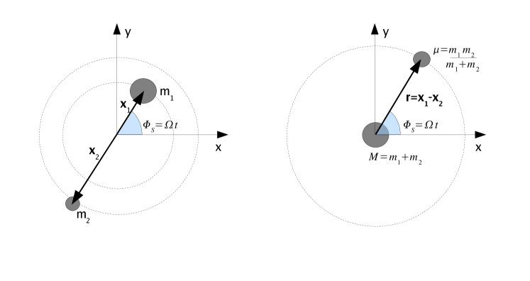
Figure 1.1: The left plot shows a binary with masses $m_{1}$ and $m_{2}$ at positions $\mbox{\boldmath$x$}_{1}$ and $\mbox{\boldmath$x$}_{2}$ measured from their common centre of mass which we use as the origin. The bodies orbit their common centre of mass with orbital frequency $\Omega$. The right hand plots shows the equivalent system where we only consider the motion of a single body with mass equal to the reduced mass $\mu=m_{1}m_{2}/(m_{1}+m_{2})$ of the binary which orbits the centre of mass at position $\mbox{\boldmath$r$}\equiv\mbox{\boldmath$x$}_{1}-\mbox{\boldmath$x$}_{2}$ [95].

For our binary we will have

$$r^{x}(t) = r\cos(\Omega t)$$ (1.66)

$$r^{y}(t) = r\sin(\Omega t)$$ (1.67)

$$r^{z}(t) = 0$$ (1.68)

where $r\equiv|\mbox{\boldmath$r$}|$. Taking the time derivative of the mass-quadrupole $I^{ij}$ twice and using the centripetal acceleration $\ddot{r}^{i}=-(|\dot{\mbox{\boldmath$r$}}^{2}|/|\mbox{\boldmath$r$}|)\hat{r}^{i}$ we find

$$\bar{h}^{ij}=\frac{4}{D}\mu|\dot{\mbox{\boldmath$r$}}^{2}|\left(\hat{\dot{r}}^{i}\hat{\dot{r}}^{j}-\hat{r}^{i}\hat{r}^{j}\right)$$ (1.69)

Taking the time derivatives of $r$:

$$\dot{r}^{x}(t) = -\Omega r\sin(\Omega t)$$ (1.70)

$$\dot{r}^{y}(t) = \Omega r\cos(\Omega t)$$ (1.71)

$$\dot{r}^{z}(t) = 0.$$ (1.72)

we can then write the metric perturbation as

$$\bar{h}^{ij}=-\frac{4\Omega^{2}\mu r^{2}}{D}\left(\begin{array}[]{ccc}\cos[2\Omega(t-D)]&\sin[2\Omega(t-D)]&0\\ \sin[2\Omega(t-D)]&-\cos[2\Omega(t-D)]&0\\ 0&0&0\\ \end{array}\right).$$ (1.76)

We will briefly discuss the properties of gravitational waves from binary systems. Intuitively we can imagine that as system loses energy to gravitational waves its orbit will shrink. This is referred to as the inspiral of a binary. Note that in Newtonian gravity, no gravitational waves would be emitted, the system would not lose energy and the inspiral would not occur. From Kepler’s third law, the shrinkage of the binaries orbit will cause the period to decrease. From Eq. (1.64) we see that as the period decreases the gravitational wave amplitude will increase. From Eq. (1.76) we see that the gravitational wave frequency is proportional (twice) to the frequency of sources orbit . Therefore, as period decreases the orbital frequency and therefore gravitational wave frequency will also increase. Consequently gravitational waves emitted during the inspiral of a binary system is described as chirp since they increase in both amplitude and frequency with time.

1.3 Detection of gravitational waves

We consider freely-falling test masses (i.e., with no force applied). The co-ordinate position of the freely-falling test masses will remain constant as a gravitational wave passes. However, since the metric changes we can observe a change in the proper distance between two freely falling test masses. Initially we consider only the $+$ polarization components of the metric perturbation in Eq. (1.53). Remembering the form of the metric with only small perturbations $g_{\alpha\beta}(\mbox{\boldmath$x$})=\eta_{\alpha\beta}+h_{\alpha\beta}(\mbox{\boldmath$x$})$ we can write the proper separation $ds$ in terms of the co-ordinate separation $dt,dx,dy,dz$ between two events as

$$ds^{2} = g_{\alpha\beta}(\mbox{\boldmath$x$})dx^{\alpha}dx^{\beta}$$ (1.77)

$$= -dt^{2}+[1+h_{xx}]dx^{2}+[1-h_{xx}]dy^{2}+dz^{2}$$ (1.78)

for a plus polarized gravitational wave propagating in the $z$-direction.

Now we consider a freely-falling test mass initially at a co-ordinate distance $L_{x(\rm{co-ord})}$ along the $x$-axis from the origin. We evaluate the proper distance between them in the $x$-direction (at time $t$ at $z=0$):

$$L_{x}(t)=\int_{0}^{L_{x(\rm{co-ord})}}[1+h_{xx}(t,0)]^{1/2}dx\sim L_{x(\rm{co-ord})}\left[1+\frac{1}{2}h_{xx}(t,0)\right]$$ (1.79)

where we have used the binomial expansion to approximate the right hand side. The time-dependent variation in the proper distance between test masses along $x$-axis is given by

$$\delta L_{x}(t)=\frac{1}{2}L_{x(\rm{co-ord})}h_{xx}(t,0).$$ (1.80)

Note that in flat space ($h_{\alpha\beta}=0$) the co-ordinate separation $L_{x(\rm{co-ord})}$ will be equal to the (constant) proper distance $L_{x}$ between the particles along the $x$-axis (since $\eta_{ii}=1$). Rewriting Eq. (1.80) as

$$\frac{\delta L_{x}(t)}{L_{x(\rm{co-ord})}}=\frac{1}{2}h_{xx}(t,0)$$ (1.81)

we identify the left hand side as a dimensionless strain along the $x$-axis caused by the passing of the gravitational wave. We can generalise this to

$$\frac{\delta L(t)}{L}=\frac{1}{2}h_{ij}(t,0)n^{i}n^{j}$$ (1.82)

where $n$ is a unit vector in the $x-y$ plane and $L$ would be the proper distance in flat space (equal to the co-ordinate separation).

The strains caused by the plus polarization part of the gravitational wave emitted by a binary system (see Eq. (1.76)) and propagating in the $z$-direction are given by:

$$\frac{\delta L_{x}(t)}{L_{x(\rm{co-ord})}} = -\frac{2\Omega^{2}\mu r^{2}}{D_{z}}\cos[2\Omega(t-D_{z})]$$ (1.83)

$$\frac{\delta L_{y}(t)}{L_{y(\rm{co-ord})}} = +\frac{2\Omega^{2}\mu r^{2}}{D_{z}}\cos[2\Omega(t-D_{z})]$$ (1.84)

$$\frac{\delta L_{z}(t)}{L_{z(\rm{co-ord})}} = 0.$$ (1.85)

As expected, since we are are in the Transverse Traceless gauge we have no strain in the direction of the waves propagation (i.e., no longitudinal strain) and we have (sinusoidal) oscillations in the plane transverse to the waves propagation. Note the difference in sign in the strains caused along the $x$ and $y$ directions. This indicates that as the gravitational wave causes proper distances in the $x$-direction to increase it simultaneously causes proper distances in the $y$-direction to decrease (and vice versa). The top plot of Fig. 1.2 shows the effect of a plus polarized gravitational wave propagating in the $z$-direction on a ring of freely falling test masses.

For a cross polarized gravitational wave propagating in the $z$-direction we can write the proper separation $ds$ in terms of the co-ordinate separation $dt,dx,dy,dz$ between two events as

$$ds^{2} = g_{\alpha\beta}(\mbox{\boldmath$x$})dx^{\alpha}dx^{\beta}$$ (1.86)

$$= -dt^{2}+dx^{2}+dy^{2}+2h_{xy}\,dx\,dy+dz^{2}.$$ (1.87)

We will now show that a cross polarized gravitational wave will have similar effect on a ring of freely falling test masses as a plus polarized gravitational wave if we rotate our axes by $45^{\circ}$. Consider rotating the $x$ and $y$ axes through $45^{\circ}$ about the $z$-axis:

$$x\rightarrow x^{\prime} = \frac{1}{\sqrt{2}}(x+y)$$ (1.88)

$$y\rightarrow y^{\prime} = \frac{1}{\sqrt{2}}(x-y)$$ (1.89)

which lead to the identities

$$2dxdy = dx^{\prime 2}-dy^{\prime 2}$$ (1.90)

$$dx^{2}+dy^{2} = dx^{\prime 2}+dy^{\prime 2}.$$ (1.91)

Rewriting the proper separation (Eq. (1.86)) using these identities we find it has the same form as the proper separation caused by a plus polarized gravitational wave in un-rotated axes:

$$ds^{2} = -dt^{2}+[1+h_{xy}]dx^{\prime 2}+[1-h_{xy}]dy^{\prime 2}+dz^{2}$$ (1.92)

The bottom plot of Fig. 1.2 shows the effect of a cross polarized gravitational wave propagating in the $z$-direction on a ring of freely falling test masses.

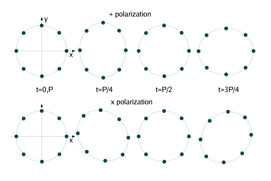
Figure 1.2: Plots showing the change in positions of a ring of test masses in the $x-y$ plane as gravitational wave propagates in the $z$-direction. The top plot shows the effect of a plus ($+$) polarization gravitational wave. Over the course of a single period $P$ of this gravitational wave the ring of test masses is contracted in the $x$ direction and simultaneously expanded in the $y$ direction (at $P/4$) direction and then expanded in the $x$ direction and simultaneously contracted in the $y$ direction (at $3P/4$). The bottom plot shows the effect of a cross ($\times$) polarization gravitational wave. Its effect on the ring of masses is equivalent to the plus polarization waveform rotated through $45^{\circ}$. In this plot the expansion and contraction of the ring of masses has been exaggerated and is far greater than we would expect from a typical gravitational wave.

1.3.1 Gravitational wave detectors

The search for gravitational waves is dominated by two different types of detector, resonant bars and laser-interferometers. Resonant bar detectors typically consist of a massive metal cylinder which has been cryogenically cooled. A passing gravitational wave will cause stretching and contraction of the bar which can be measured (see Mauceli et al. (1996) [99] for a description of the Allegro detector). These detectors have best sensitivity to gravitational waves with frequencies in a narrow band about their own resonant frequencies, typically $\sim 900$ Hz (see Table 1 of Astone et al. (2003) [16]). We will find that many sources of gravitational waves including the inspiral of binaries will emit across a wide range of frequencies. Whereas resonant bar detectors achieve good sensitivity over only a relatively narrow band of frequencies, laser interferometers have good sensitivity over a broad band of frequencies and it is these detectors that we shall focus upon.

Despite not being ideal for searches for gravitational waves from the inspiral of binaries, resonant bars have been used for searches for gravitational waves with unknown form and/or short duration and bandwidth. For a review of gravitational wave searches using resonant bar detectors see Astone et al. (2003) [16]. Recent searches for gravitational wave stochastic background and short duration gravitational wave bursts using both resonant bar and laser interferometers are described in Abbott et al. (2007) [58] and Baggio et al. (2008) [59] (see Fig. 2 of this paper for a comparison of the sensitivities of these different types of detector).

A Michelson interferometer with arms along the $x$ and $y$ directions is shown in the upper plot of Fig. 1.3. The interferometer works as follows: the laser source sends a laser beam to a beam-splitter which splits it into two coherent beams which then travel at right angles to each other along the interferometers arms. The laser beams are reflected back by mirrors at the end of each arm and are recombined at the beam-splitter which then directs the recombined beam to a photodetector which measures its intensity.

The two mirrors and the beam-splitter behave similarly to the test masses shown in Fig. 1.2 and move accordingly with the passing of a gravitational wave. We measure the movement of the two mirrors and the beam-splitter through the intensity of the recombined laser beam measured at the photodetector. The real gravitational wave detectors that we will discuss shortly are designed so that when there is no gravitational wave (i.e, the mirrors have proper distances $L_{x}=L_{y}$ from the beam-splitter) the laser beams interfere destructively and we measure a dark fringe at the photodetector.

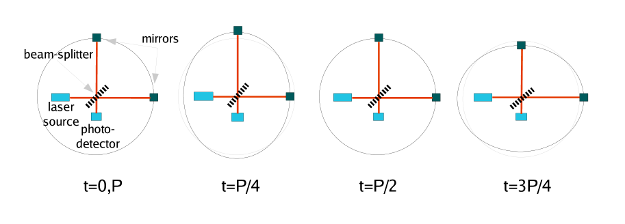
Figure 1.3: Plot showing the effect of a plus polarization gravitational wave on a simple Michelson interferometer. The gravitational wave causes the interferometers mirrors to move similarly to the test masses in the upper plot of Fig. 1.2. The interferometer is designed so that when it is in its unperturbed configuration the laser beams reflected along the $x$ and $y$ arms will destructively interfere when recombined at the beam-splitter (at $t=0,P/2,P\dots$) and a dark fringe will be measured by the photodetector. A passing gravitational wave would cause variation in the proper distance between the beam-splitter and the mirrors enabling detection of the gravitational wave through measurement of the intensity of the recombined laser beam.

Constructive interference will occur when the difference in the path travelled by the laser is $\Delta L=n\lambda$ where $\lambda$ is the wavelength of the laser (assumed to be monochromatic) and $n=0,1,2\dots$. Destructive interference occurs when $\Delta L=(n+1/2)\lambda$. The path difference between the laser beams travelling along the $x$ and $y$ arms can be written

$$\Delta L=2L_{x}-2L_{y}-\frac{\lambda}{2}$$ (1.93)

where $L_{x}$ and $L_{y}$ are the proper distances of the mirrors from the beam-splitter (the prefactor of 2 indicating that the laser beam makes a return trip) and the subtraction of $\lambda/2$ ensures we have destructive interference when $L_{x}=L_{y}$ .

From our equations for the strain caused by a passing gravitational wave (e.g., Eq. (1.82)) we can see that by increasing the length of the interferometers arms ($L$) we will increase the strain we are seeking to measure ($\delta L(t)$).

From Eq. (1.86) for the proper separation caused by a cross polarization gravitational wave we can see that the it will not be detectable by the interferometer we have shown in Fig. 1.3: the strain it induces will cause the $x$ and $y$ arms of the interferometer to extend and compress equally and at the same time as each other. Therefore the path travelled by the laser beams will remain equal $L_{x}(t)=L_{y}(t)$ and we would always measure a dark fringe at the photodetector. Equally, if we rotated the interferometer in Fig. 1.3 by $45^{\circ}$ it would be sensitive to only cross polarization gravitational waves but not to plus polarization waves.

1.3.2 Characterising the detectors

We characterise gravitational wave detectors by their power or amplitude spectral density. $S_{h}(f)$ is the noise power spectral density per $\rm{Hz}$ of a data stream. $S_{h}^{\rm{one-sided}}(f)=2S_{h}^{\rm{two-sided}}(f)$. The amplitude spectral density $S_{h}(f)^{1/2}$ is the square root of the power spectral density and has units $\rm{Hz}^{-1/2}$. We will discuss the power density in the context of data analysis in Sec. 1.4. Figure 1.4 shows the amplitude spectral density curves for a number of current and planned laser interferometric gravitational wave detectors. Figure 1.5 shows the best amplitude spectral density curves obtained by LIGO during each of its first five science runs. Lower values of amplitude spectral density indicate sensitivity to smaller strains and we shall see that $S_{h}(f)$ appears in the denominator of our equation for signal to noise ratio (see Sec. 1.4).

From our equations for the emission of gravitational waves (see e.g., Eq. (1.76)) we can see that the amplitude of the strain caused will be proportional to the inverse of the distance from the source to the detector. Therefore, sensitivity to smaller strain means sensitivity to more distant sources. Improvements in sensitivity (i.e., reductions in $S_{h}(f)$) by a factor $x$ would lead to a proportional increase in the distance to which a given source could be observed with a particular strain and therefore a factor $x^{3}$ increase in the volume to which we could observe the source.

In this thesis we present results from the analysis of data collected by the Laser Interferometer Gravitational-wave observatory (LIGO) and develop an algorithm to be used with data collected by the Laser Interferometer Space Antenna (LISA). We will now briefly describe these detectors.

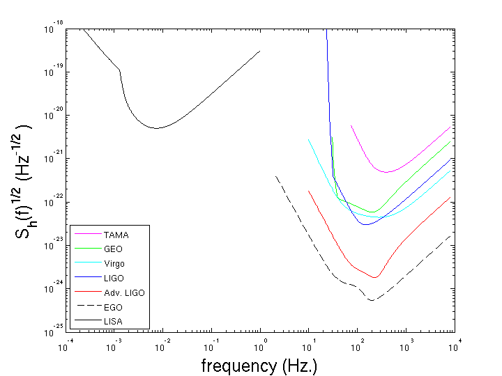
Figure 1.4: Amplitude spectra of current (TAMA, GEO, LIGO, Virgo) and planned (Advanced LIGO, EGO, LISA) laser-interferometric gravitational wave detectors at their design sensitivities. Fits to the TAMA, GEO and LIGO data were published in Damour et al. (2001) [53]. The noise curve data was provided by M.-K. Fujimoto (TAMA), G.Cagnoli and J. Hough (GEO) and K. Blackburn (LIGO). The Virgo noise curve data was provided by J-Y. Vinet (available on Virgo home page [142]). The Advanced LIGO noise curve data was provided by Kip Thorne and the fit by B.S.Sathyaprakash. The EGO noise curve is given by Van Den Broeck and Sengupta (2007) [35]. The LISA noise curve is given by Barack and Cutler (2004) [20].

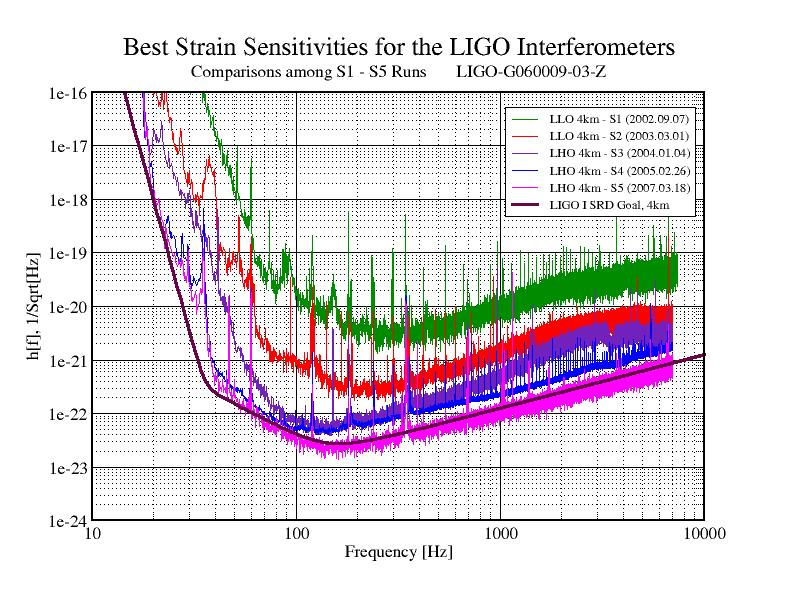
Figure 1.5: Plot showing the best (lowest) amplitude spectra obtained by LIGO during each of its first five science runs. The design sensitivity curve is also shown. We see a steady improvement in LIGO’s best sensitivity as we progress through the science runs and in November 2005, during its fifth science run (S5), LIGO achieved its design sensitivity above $\sim 50$ Hz. In contrast to the smooth shape of the design sensitivity curve, the real spectra include sharp spikes in which the detector has reduced sensitivity over a narrow band of frequencies. These narrow-band spectral lines are caused by vibrations in the wires used to suspend the interferometer’s mirrors (“violin modes”), laser noise and harmonics to the U.S. power mains frequency of $60$ Hz [51]. Methods for removing these lines are described in Searle et al. (2003) [129]. This figure was created by the LIGO Laboratory and has been assigned LIGO document number LIGO-G06009-03-Z [96].

1.3.3 LIGO

The Laser Interferometer Gravitational-wave Observatory (LIGO) consists of three detectors located at two sites across the US. The LIGO Hanford Observatory (LHO) in Washington state consists of two co-located interferometers of arm length 4km and 2km and are known as H1 and H2 respectively. The LIGO Livingston Observatory (LLO) in Louisiana consists of a single 4km interferometer known as L1. See Abbott et al. (2004) [137] for a more detailed description of the LIGO detectors.

The sensitivity of ground-based laser interferometric detectors is primarily limited by three different sources of noise, seismic disturbances at low frequencies, thermal noise at intermediate frequencies and shot noise, caused by statistical fluctuations in the laser power, at high frequencies. For a detailed breakdown of the various sources of noise which contribute to LIGO’s amplitude spectrum see Sigg (2008) [65]. Figure 1.6 shows a schematic layout of a LIGO interferometer. The main additions to the LIGO interferometers beyond the simple Michelson interferometer described in Sec. 1.3.1 are i) the second set of test mass mirrors along the interferometer arms which form a Fabry-Perot optical cavity with the test mass mirrors at the ends of the arms and ii) the power recycling mirror between the beam-splitter and the laser source. The goal of these extra mirrors is to increase the time that the laser beam spends in each of the interferometer’s arms. When the interferometer is “locked” into resonance, i.e., its mirrors are positioned correctly, the laser beam will bounce back and forth $\sim 50$ times in the optical cavity in each arm. This effectively increases the arm lengths of the interferometer and therefore improves its strain sensitivity (see, for example, Eq. 1.80) [64]. When the mirrors are not correctly positioned we described the interferometer as being “unlocked” (see Sec. 2.6.1). When the interferometer is locked and the arms are not being disturbed by environmental noise or a passing gravitational wave, almost all of the laser light will return from the arms to the beam-splitter and back towards the laser source. The power recycling mirror reflects this laser light back towards the beam-splitter and into the arms of the interferometer, effectively increasing the laser power by a factor of $\sim 40$ [67] which will reduce the level of shot noise [137].

Construction of LIGO began in 1994 and was substantially completed in 2000. During October 2002 LIGO and GEO took part in the first science run (S1) [137]. No gravitational waves were observed. Although neither detector had achieved their design sensitivities (see Fig. 1.5), LIGO had sufficiently good sensitivity to be able to set a better (i.e. lower) upper limit on the rate of coalescences of binary neutron star inspirals than previous experiments [2] (the process of setting upper limits on the rate of coalescences in the event that no gravitational waves were observed is discussed later in Sec. 2.8). In November 2005 LIGO achieved its design sensitivity above $\sim 50$ Hz. In this thesis we will describe a search of LIGO data taken during its third science run (S3) which took place between October 2003 and January 2004.

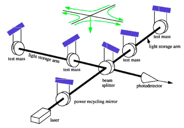
Figure 1.6: A schematic layout of a LIGO interferometer showing Fabry-Perot optical cavities and power recycling (see Sec. 1.3.3). This figure was reproduced from B. Abbott et al., Nucl. Instrum. Meth. A 517 (2004) 154-179 [137] with permission from the authors.

1.3.4 LISA

The Laser Interferometer Space Antenna (LISA) will consist of three spacecraft in heliocentric Earth-trailing orbits, $5$ million kilometres apart at the corners of an (approximately) equilateral triangle (see Danzmann K et al. (1998) [60] for a full description of the mission). Each of LISA’s spacecraft house freely falling test masses. A passing gravitational wave will change the (proper) distance between these test masses. There will be two lasers running between each pair of spacecraft, one in each direction, and, similarly to ground-based detectors such as LIGO, it is the differences in laser phase between the various light travel paths that indicate that gravitational waves are passing through the detector.

However, unlike ground-based detectors LISA will not suffer from low frequency noise caused by seismic activity and has been designed to have best sensitivity in the frequency range $\sim 10^{-4}-10^{-1}\rm{Hz}$. In the raw data, the laser phase difference is totally dominated by laser frequency noise. However, this can be suppressed without eradicating the gravitational wave signal using Time Delay Interferometry (TDI, see for instance Vallisneri (2005) [141] and references therein).

LISA is a joint NASA/ESA project and is one of five space-based observatories that form NASA’s Beyond Einstein programme. After the last review (2007) [47] the LISA Pathfinder mission, a precursor mission to LISA designed to test its key technologies, is expected to be launched in 2009. While no firm date has been set for the launch of LISA itself it is hoped to be within the next decade or so. Once launched LISA will spend around 13 months getting into its orbit and will then collect data for between 3 and 5 years.

In Sec. 3 we find that through use of time-frequency data analysis techniques LISA will be sensitive to the inspiral of stellar mass objects into supermassive black holes up to distances of a few Gpc, the merger of supermassive black holes at cosmological distances $z\sim 3.5$ and the inspiral of binary white dwarfs in the nearby universe.

1.4 Data analysis

In this Section we will describe the data analysis methods used in order to detect a gravitational wave signal in noisy data. We will consider a data stream $x(t)$ which may either contain only noise $n(t)$ or noise and a gravitational wave signal $s(t)$. We discretely sample the data stream with an interval $\Delta t$ so that $x_{j}=x(t_{j})$ where $t_{j}=j\Delta t$.

Our data analysis can be viewed within the framework of a hypothesis test. We have two hypotheses:

• $\mathcal{H}_{0}$: our null hypothesis is that there is no signal present, $x(t)=n(t)$

• $\mathcal{H}_{1}$: a signal is present in the data, $x(t)=n(t)+s(t)$

There are two types of error associated with this test:

• Type I error: rejecting $\mathcal{H}_{0}$ when it is true. In this case our analysis would infer a signal was present when there was no signal present. We refer to this type of error as a false alarm.

• Type II error: accepting $\mathcal{H}_{0}$ when it is false. In this case our analysis would not infer a signal was present when a signal was present. We refer to this type of error as a false dismissal.

It is not possible to decrease the probability of false alarm and false dismissal simultaneously; decreasing the probability of a false alarm would increase the probability of a false dismissal and vice versa.

We can approach the problem of choosing a detection method in two different ways. When taking the Neyman-Pearson approach, the probability of false dismissal is minimized having chosen a particular value for the false alarm probability. When taking the Bayesian approach, the probability of the null hypothesis is estimated in advance and penalties are assigned to describe the relative severity of false alarms and false dismissals occurring. These pieces of information are used to construct the Bayes risk which is subsequently minimized (see, for example, Whalen (1971) [149]).

Significantly both approaches yield a likelihood ratio test of the form:

$$\mathcal{H}_{0} \;\mathrm{if}\;\;\Lambda<\gamma$$ (1.94)

$$\mathcal{H}_{1} \;\mathrm{if}\;\;\Lambda\geq\gamma$$ (1.95)

$$\mathrm{where} \;\Lambda=\frac{p(x;\mathcal{H}_{1})}{p(x;\mathcal{H}_{0})}$$ (1.96)

where $p(x;y)$ is the probability of $x$ occurring given that $y$ is true and where $\gamma$ is some thresholding value. The form of this threshold will depend on whether the Neyman-Pearson or Bayesian approach is taken. The quantity $\Lambda$ is called the likelihood ratio.

We will now consider the case where the noise $n(t)$ is Gaussian process with a mean of zero, i.e., $\overline{n(t)}=0$ where we use an overbar to denote ensemble average. The noise can be characterised equivalently by either its autocorrelation $r(t-t^{\prime})$ or by its (one-sided) power spectral density $S_{n}(f)$. Indeed, the Wiener–Khinchin theorem (also known as the Wiener–Khintchine or Khinchin-–Kolmogorov theorem) shows that for any stationary process (i.e., one which can be described at any time by the same probability distribution) the power spectral density is simply the Fourier transform of its autocorrelation function.

The real, one-sided noise power spectral density is given by

$$\overline{\tilde{n}(f)\tilde{n}^{*}(f^{\prime})}=\frac{1}{2}\delta(f-f^{\prime})S_{n}(|f|).$$ (1.97)

In simple terms, the autocorrelation function simply measures the correlation between $n(t)$ at two different times.

The multivariate Gaussian probability density function of our data when there is no signal present (i.e., $x(t)=n(t)$ and $\overline{x(t)}=\overline{n(t)}=0$) can be written

$$p(\mbox{\boldmath$x$};\mathcal{H}_{0})=\frac{1}{(2\pi)^{N/2}|\mbox{\boldmath$C$}|^{1/2}}\mathrm{exp}\left[-\frac{1}{2}(\mbox{\boldmath$x$})^{T}\mbox{\boldmath$C$}^{-1}(\mbox{\boldmath$x$})\right]$$ (1.98)

where $C$ is the covariance matrix of the $x_{j}$ and $|\mbox{\boldmath$C$}|$ is the determinant of $C$. Following the derivation in Section 2A of Finn (1992) [62] we find that through use of the Wiener–Khinchin theorem and Parseval theorem that we can write this probability in the continuum limit as

$$p(\mbox{\boldmath$x$};\mathcal{H}_{0})=\frac{1}{(2\pi)^{N/2}|C_{n,ij}|^{1/2}}\mathrm{exp}[-\left<x,x\right>)]$$ (1.99)

where we have defined the (symmetric) inner product for any two functions $g$ and $h$ to be

$$\left<g,h\right>\equiv\int_{-\infty}^{\infty}\left[\tilde{g}(f)\tilde{h}^{*}(f)+\tilde{h}(f)\tilde{g}^{*}(f)\right]\frac{df}{S_{n}(f)}.$$ (1.100)

For a real signal $h(t)$ is real we have $\tilde{h}^{*}(f)=\tilde{h}(-f)$ . If both $h(t)$ and $g(t)$ are real we can write

$$\left<g,h\right> = 2\int_{-\infty}^{\infty}\tilde{g}^{*}(f)\tilde{h}(f)\frac{df}{S_{n}(|f|)}$$ (1.101)

$$= 4\Re\int_{0}^{\infty}\tilde{g}^{*}(f)\tilde{h}(f)\frac{df}{S_{n}(f)}.$$ (1.102)

For real functions $h(t)$ and $g(t)$ we can also equivalently write

$$\left<g,h\right>\equiv 2\int_{0}^{\infty}\left[\tilde{g}(f)\tilde{h}^{*}(f)+\tilde{h}(f)\tilde{g}^{*}(f)\right]\frac{df}{S_{n}(f)}.$$ (1.103)

Since we know that $p(x;\mathcal{H}_{1})\equiv p(x-s;\mathcal{H}_{0})$ we can write

$$p(\mbox{\boldmath$x$};\mathcal{H}_{1})=\frac{1}{(2\pi)^{N/2}|\mbox{\boldmath$C$}|^{1/2}}\mathrm{exp}\left[-\frac{1}{2}(\mbox{\boldmath$x$})^{T}\mbox{\boldmath$C$}^{-1}(\mbox{\boldmath$x$})\right]$$ (1.104)

Rewriting the inner product

$$\left<x-s,x-s\right>=\left<x,x\right>+\left<s,s\right>-2\left<s,x\right>$$ (1.105)

we can find the likelihood ratio

$$\Lambda=\mathrm{exp}[2\left<s,x\right>-\left<s,s\right>].$$ (1.106)

The inner product of the signal with itself $\left<s,s\right>$ is clearly not dependent on the data $x(t)$ and we can choose to rewrite our statistical test using the likelihood ratio with this term removed. Also since our expression for the likelihood ratio will then be a monotonic function of the exponent we can go further and rewrite our test as

$$\mathcal{H}_{0} \;\mathrm{if}\;\;\left<s,x\right><\gamma_{*}$$ (1.107)

$$\mathcal{H}_{1} \;\mathrm{if}\;\;\left<s,x\right>\geq\gamma_{*}$$ (1.108)

where $\gamma_{*}$ is some thresholding value.

Matched-filtering is the optimal technique for the detection of a known signal in stationary, Gaussian noise. The optimal filter $q=h/S_{n}(f)$ consists of an accurate representation of the expected signal, which we call the template $h$, weighted by the noise spectrum of the detector $S_{n}(f)$ so that there are greater contributions to the inner product $\left<x,h\right>$ when the detector has good sensitivity (i.e., when $S_{n}(f)$ is small) [17].

1.4.1 Properties of the inner product

The mean of $\left<x,h\right>$ for an ensemble of $x$ is given by

$$\overline{\left<x,h\right>}=2\int_{-\infty}^{\infty}\overline{\tilde{x}^{*}(f)}\tilde{h}(f)\frac{df}{S_{n}(f)}$$ (1.109)

where since the template $h$ is stationary we have $\overline{\tilde{h}(f)}=\tilde{h}(f)$.

In the absence of signal $x(t)=n(t)$ we find

$$\overline{\left<n,h\right>}=2\int_{-\infty}^{\infty}\overline{\tilde{n}^{*}(f)}\tilde{h}(f)\frac{df}{S_{n}(f)}=0$$ (1.110)

as long as $\overline{n(t)}=0$. The variance of $\left<x,h\right>$ for an ensemble of $x$ is given by

$$\overline{\left[\left<x,h\right>-\overline{\left<x,h\right>}\right]^{2}}.$$ (1.111)

Again, assuming there is no signal we find

$$\overline{\left[\left<n,h\right>-\overline{\left<n,h\right>}\right]^{2}}=\overline{\left[\left<n,h\right>\right]^{2}}$$ (1.112)

since we have found previously that $\overline{\left<n,h\right>}=0$. From Eqs. (1.100) and (1.103) we can see that $\left<a,b\right>\equiv\left<b,a\right>$. Therefore we can write

$$\overline{\left[\left<n,h\right>\right]^{2}} = \overline{\left<n,h\right>\left<h,n\right>}$$ (1.113)

$$= 4\overline{\int_{-\infty}^{\infty}\int_{-\infty}^{\infty}\tilde{n}^{*}(f)\tilde{h}(f)\tilde{h}^{*}(f^{\prime})\tilde{n}(f^{\prime})\frac{df}{S_{n}(f)}\frac{df^{\prime}}{S_{n}(f^{\prime})}}$$ (1.114)

$$= 4\int_{\infty}^{\infty}\int_{\infty}^{\infty}\overline{\tilde{n}^{*}(f)\tilde{n}(f^{\prime})}\tilde{h}^{*}(f^{\prime})\tilde{h}(f)\frac{df}{S_{n}(f)}\frac{df^{\prime}}{S_{n}(f^{\prime})}$$ (1.115)

$$= 4\int_{\infty}^{\infty}\int_{\infty}^{\infty}\frac{1}{2}\delta(f-f^{\prime})S_{n}(f)\tilde{h}^{*}(f^{\prime})\tilde{h}(f)\frac{df}{S_{n}(f)}\frac{df^{\prime}}{S_{n}(f^{\prime})}$$ (1.116)

$$= \left<h,h\right>$$ (1.117)

If we assume that our template is normalised such that $\left<h,h\right>=1$ we will therefore find that the variance of $\left<n,h\right>$ is unity.

If we perform the same analysis when the detector data consists of signal and noise, i.e., $x(t)=h(t)+n(t)$ (where we will assume our template $h(t)$ is a perfect description of out signal) we find the mean of the overlap is given by

$$\overline{\left[\left<x,h\right>\right]} = \overline{\left[\left<n+h,h\right>\right]}$$ (1.118)

$$= \overline{\left[\left<n,h\right>\right]}+\overline{\left[\left<h,h\right>\right]}$$ (1.119)

$$= 1$$ (1.120)

and that the variance is given by

$$\overline{\left[\left<x,h\right>-\overline{\left<x,h\right>}\right]^{2}} = \overline{\left[\left<n,h\right>\right]^{2}}$$ (1.121)

$$= 1.$$ (1.122)

It is also trivial to see how the amplitude of an incoming signal can be measured immediately from the inner product. Consider a template $h(t)$ and a signal $s(t)=Ah(t)$ where $A$ is a real, dimensionless and time-independent number. We find simply that the mean output of our template with data consisting of signal $Ah(t)$ and noise $n(t)$ is

$$\overline{\left[\left<x,h\right>\right]} = \overline{\left[\left<n,h\right>\right]}+\overline{\left[\left<h,Ah\right>\right]}$$ (1.123)

$$= A.$$ (1.124)

1.4.2 Definition of signal to noise ratio

We define the signal to noise ratio (SNR) $\rho$ as the statistic $\left<x,h\right>$ divided by its standard deviation. Using the results from the previous Section we find that when our data $x$ contains a signal and stationary, Gaussian noise, $x(t)=n(t)+s(t)$ that the expectation value of the SNR is $\overline{\rho}=\left<s,h\right>$ (assuming that we have normalised our templates such that $\left<h,h\right>=1$). If our data $x$ contains stationary, Gaussian noise but no signal, $x(t)=n(t)$ then $\overline{\rho}=0$. In practise the detector noise will be neither stationary nor Gaussian. In order to account for the non-stationarity of the detector noise, we estimate the noise spectrum $S_{n}(f)$, used within the calculation of $\left<x,h\right>$, at regular intervals. Environmental disturbances and problems with the detector itself can cause transient artefacts in the detector data meaning that it will become non-Gaussian. The detector is continuously monitored allowing data obtained during times of a known environmental disturbance or problem with the detector to be excluded from subsequent data analysis. Details on the methods used to search for gravitational wave signals in real detector data using matched-filtering is discussed further in Sec. 2.6. In Sec. 5.1.2 we shown that the linear transformation (e.g., the matched-filtering) of a multivariate Gaussian distribution is also a multivariate Gaussian distribution. We will use this property later when testing our matched-filter algorithm in Sec. 2.4.2.

Chapter 2 Searching for precessing binary systems in LIGO data

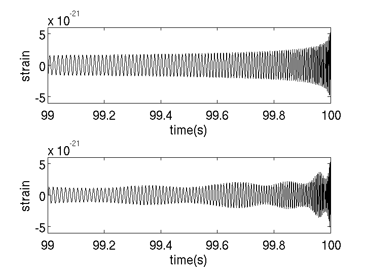
Figure 2.4: The gravitational waveforms we expect to observe from the late inspiral phase of two different neutron star - black hole systems, one consisting of non-spinning bodies (upper plot) and the other consisting of maximally spinning bodies (lower plot). Both systems are identical apart from the spin of their component bodies. The spin-induced precession of the binary’s orbital plane causes modulation of the gravitational wave signal and can be clearly seen in the lower plot.

Interaction between the spins of the binary’s component bodies and the orbital angular momenta will cause its orbital plane to precess during the course of the system’s evolution. Figures 2.4 and 2.5 compare the waveforms that would be observed from similar binaries, one consisting of non-spinning components and the other consisting of spinning components. It has been found that optimal matched-filter searches should use templates which take into account the spin modulation of gravitational waves. In this Chapter we will we summarise how stellar mass binaries (i.e., those which LIGO is sensitive to) form and how their components spin up (Sec. 2.1), then move onto modelling their inspiral orbits and gravitational wave emissions (Sec. 2.2). We then summarise the progress that has been made in building detection efficient templates to capture these systems (Sec. 2.3). The remainder of the Chapter details the use of the BCV2 detection template family (Sec. 2.4) to search for signals emitted by binaries with spinning components in data taken by LIGO during its third science run. No detections were made and in Sec. 2.8 we calculate upper limits on the rate of coalescence of neutron star - black hole binaries with spinning components.

The analysis of LIGO data described in the latter part of this Chapter was led by the author (Gareth Jones) as a member of the LIGO Scientific Collaboration/Virgo Compact Binary Coalescence working group [97] and has been previously published in B. Abbott et al. (2007) [46].

2.1 Formation and evolution of stellar mass binary systems

We briefly review the current literature regarding the formation and evolution of binary systems paying particular attention to the spins of the binary’s components. The literature focuses upon NS-BH binaries and it turns out that the effects of spin are more pronounced in systems with small mass ratio (i.e., unequal masses). It is likely that the formation and evolution of other stellar mass binaries consisting of compact objects, e.g., BH-BH and NS-NS systems will be qualitatively similar and the discussion here will be relevant to all these cases.

Stellar mass BHs form either through the collapse of a massive progenitor (e.g. a main sequence star that has exhausted the hydrogen in its core) or via the accretion-induced collapse of a NS (which itself will have formed via collapse of a massive progenitor). After core collapse, progenitor stars with mass $<1.4M_{\odot}$ become White Dwarfs, those with mass in the range $1.4$ to $\sim 3M_{\odot}$ become NSs and those with mass $\gtrsim 3M_{\odot}$ become BHs.

As internal densities of a progenitor star collapsing under gravity exceed $~{}10^{10}\rm{kg\,m}^{-3}$ the majority of its protons and electrons will undergo inverse beta decay to form neutrons (and neutrinos). In neutron stars it is the repulsive forces (arising from degeneracy pressure as described by the Pauli exclusion principle) between the neutrons that resist further gravitational collapse. For progenitor stars with mass $\gtrsim 3M_{\odot}$ the gravitational forces exceed the outward degeneracy pressure forces and the star will collapse further to become a black hole.

A black hole is defined by its event horizon whose radius will depend on its mass and spin only. In classical physics anything falling through the event horizon can never return from behind it (in quantum physics there are exceptions to this statement such as the postulated Bekenstein-Hawking radiation). Theoretically, black holes are created when any quantity of matter collapses under gravity and becomes smaller than its event horizon. In nature there is evidence for stellar mass and supermassive black holes, both of which are expected to play leading roles in the production of the gravitational waves we expect to observe with current and planned detectors. Black holes contain a physical singularity, a point where the curvature of spacetime is infinite and physics breaks down (physical singularities are different from co-ordinate singularities). The “no hair” theorem states that a black hole can be fully described by its mass, angular momentum and charge.

The formation of a typical NS-BH binary will begin with two main sequence stars in orbit about their common centre of mass. As the more massive of these star evolves away from the main sequence it will expand until it fills its Roche lobe before transferring mass to its companion. The Roche lobe is defined as the region of space around an object in a binary system within which orbiting material is gravitationally bound to that object. If the object expands past its Roche lobe, then the material outside of the lobe will fall into the other object in the binary.

The more massive body would eventually undergo core collapse to form a BH, and the system as a whole would become a high-mass X-ray binary. As the second body expands and evolves it would eventually fill its own Roche lobe and the binary would then go through a common-envelope phase. This common-envelope phase, characterised by unstable mass transfer, would be highly dissipative and would probably lead to both contraction and circularization of the binary’s orbit. Accretion of mass can allow the BH to spin-up. It has been argued that the common-envelope phase, and associated orbital contraction, is essential in the formation of a binary which will coalesce within the Hubble time [87]. Finally the secondary body would undergo supernova to form a NS (or if massive enough, a BH). Prior to the supernova of the secondary body we would expect the spin of the BH to be aligned with the binary’s orbital angular momentum [87]. However, the “kick” associated with the supernova of the secondary body could cause the orbital angular momentum of the post-supernova binary to become tilted with respect to the orbital angular momentum of the pre-supernova binary. Since the BH would have a small cross-section with respect to the supernova kick we expect any change to the direction of its spin angular momentum to be negligible and the BH spin to be misaligned with respect to the post-supernova orbital angular momentum [75]. The misalignment between the spin and orbital angular momentum is expected to be preserved until the system becomes detectable by ground-based interferometers [75, 125].

2.1.1 Expected merger rate of compact binaries

Estimates of the merger rates of compact binaries consistent with present astrophysical understanding are summarised in Abbott et al. (2007) [5]. The rate of merger of NS-NS binaries can be inferred by the four observed binary systems containing pulsars which will coalesce within the Hubble time [117, 103]. The current estimate of the merger rate of NS-NS systems (at $95\%$ confidence) is $10-170\times 10^{-6}\rm{yr}^{-1}\,\rm{L}_{10}^{-1}$ [89, 90, 93, 88] where $\rm{L}_{10}=10^{10}\,\rm{L}_{\odot,B}$ is $10^{10}$ times the blue light luminosity of the Sun (for reference, the luminosity of the Milky Way is around $1.7\,\rm{L}_{10}$).

Although, we predict that NS-BH and BH-BH systems form according to the scenario described previously, there is no direct astrophysical evidence for these systems. To predict the merger rate of these systems, the authors of Refs. [108, 109] considered various population synthesis models of compact binary formation which are consistent with the expected merger rate of NS-NS systems. They find that the merger rates of binary populations in galactic fields are likely to lie (at $95\%$ confidence) in the ranges $0.1-15\times 10^{-6}\rm{yr}^{-1}\,\rm{L}_{10}^{-1}$ and $0.15-10\times 10^{-6}\rm{yr}^{-1}\,\rm{L}_{10}^{-1}$ for BH-BH and NS-BH binaries respectively.

Compact binary mergers from within dense stellar clusters or associated with short, hard gamma-ray bursts would increase the expected merger rates. When binary formation in star clusters is taken into account with relatively optimistic assumptions, detection rates could be as high as a few events per year for initial LIGO [119, 68, 105].

2.1.2 Spin magnitudes

A compact object can gain spin either during its formation (through the core collapse of a massive progenitor or the accretion-induced collapse of a NS) or through subsequent accretion episodes. The dimensionless spin parameter $\chi$ is given by $|\mbox{\boldmath$J$}|/M^{2}$ where $J$ is the total angular momentum of the compact object and $M$ is its mass . For a non-spinning body we would have $\chi=0$.

Penrose’s hypothesis of cosmic censorship states that physical singularities can only occur behind an event horizon. In Kerr geometry, used to describe the spacetime surrounding the event horizon of a spinning black hole, the outermost event horizon occurs at $r=M+\sqrt{M^{2}-a^{2}}$ where $r$ is the radial Schwarzschild/Boyer-Lindquist co-ordinate (equal to the circumference of a circle centred on the central body divided by $2\pi$). For this event horizon to form we require that $a\leq M$ which is equivalent to $\chi\leq 1$. For Earth we find $\chi\sim 800$ (found by assuming that the Earth is a solid sphere and using $|\mbox{\boldmath$J$}|=I\omega$ where $I$ is the Earth’s moment of inertia and $\omega$ is the orbital frequency of its spin).

O’ Shaughnessy et al. (2005) [107] consider likely values of birth spin and then perform population synthesis in order to model the accretion histories of black holes in inspiraling binaries and to place bounds on their expected spin. Low mass BH birth spins can be estimated by considering the birth spin of similar mass NS. Through the observation of radio pulsars NS birth spins have been estimated as $\chi=|\mbox{\boldmath$J$}|/M^{2}\simeq 0.005-0.02$. However, results from simulations indicate that a large fraction of BHs in BH-NS systems were formed by the accretion-induced collapse of a NS that has undergone a common envelope phase. We would therefore expect that the BH birth spin would be dependent on the spin attained by the NS during the poorly understood common-envelope phase. Mildly recycled pulsars in NS-NS systems are believed to have been spun up during a common envelope phase yet are still measured to have fairly small spins of $\chi\leq 0.01$. Uncertainties in both the collapse and common-envelope stages of the BH evolution lead the authors of [107] to place loose bounds on BH birth spin of between $\chi=0$ and $\chi\sim 0.5$, the birth spin of a BH forming from the collapse of a maximally spinning NS.

Results from the population synthesis performed by O’ Shaughnessy et al. showed that the evolution of the majority of NS-BH binaries is dominated by accretion associated with a common-envelope phase rather than by disk accretion. Hypercritical accretion occurs when one of the binary’s components spirals through its companion’s envelope and rapidly accretes matter at super-Eddington (for photons), neutrino-cooled rates [107]. The simulations showed that even with birth spin $\chi=0$ stellar mass BHs ($M<15M_{\odot}$) can obtain significant spin $\chi\sim 0.8$ through common-envelope phase accretion. More massive objects are more difficult to spin-up, requiring larger, and consequently less likely, transfers of mass. For less massive systems, $M<4M_{\odot}$, maximal spin ($\chi=1$) could easily be obtained through accretion alone (i.e., regardless of birth spin).

In [138], Thorne calculates an upper bound for the spin of a BH. As matter accretes onto BH its spin will increase, radiation emitted by the accretion disk which is subsequently “swallowed” by the BH causes a counteracting torque which limits the BH’s spin to $\chi<0.998$. Cook et al. (1994) [48] consider a variety of NS equations of state and calculate the maximum spin the NS could have before it would break up. For NS we find that the maximal spin value is $\chi\sim~{}0.7$ .

We can infer the mass of a compact object in a binary system through observations of its companion. The mass function is defined as

$$f(m)\equiv\frac{P_{\rm{orb}}K_{2}^{3}}{2\pi G}=\frac{m_{1}\rm{sin}^{3}(\iota)}{(1+m_{2}/m_{1})^{2}}$$ (2.1)

where $m_{1}$ and $m_{2}$ are the masses of the compact object and its companion respectively, $P_{\rm{orb}}$ is the orbital period of the binary, $K_{2}$ is the velocity amplitude of the companion object and $\iota$ is the inclination angle of the binary with respect to the observer. The mass function $f(m)$ can be calculated for X-ray binaries through measurement of the amplitude velocity of the luminous companion and the orbital period. By estimating the mass of the companion $m_{2}$ and the inclination angle of the binary (e.g., through observation of jets) we can obtain a lower limit on the mass of the compact object $m_{1}$. As of 2006, there are 20 X-ray binaries known to contain a stellar mass BH (inferred through dynamical considerations) as well as a further 20 X-ray binaries that may contain a stellar mass BH [124].

The measurement of BH spin from electromagnetic observations is in progress and in Sec. (8.2) of [124] four methods are discussed. Spectral fitting of X-ray continuum data obtained from the Rossi X-ray Timing Explorer (RXTE) and the Advanced Satellite for Cosmology and Astrophysics (ASCA) was used to place a robust lower bound on the spin of the primary component (BH) of the X-ray binary GRS 1915+105. The BH with $m_{\rm{BH}}\sim 15M_{\odot}$ was found to have spin $\chi>0.98$ [100]. In Table 2.1 the inferred masses and spins of four BH systems, each belonging to an X-ray binary, are given.

Table 2.1: Measurements of the masses and spins of four BHs each of which belong to an X-ray binary system. The masses were obtained through dynamical considerations and the spins were obtained through spectral fitting of X-ray continuum data obtained using the RXTE, ASCA and BeppoSAX space telescopes.

System	$m_{\rm{BH}}$	$\chi_{\rm{BH}}$
GRS 1915+105	$\sim 14.4M_{\odot}$ [79]	$>0.98$ [100]
4U 1543-47	$\sim 9.4M_{\odot}$ [106]	$\sim 0.75-0.85$ [131]
GRO J1655-40	$\sim 6.3M_{\odot}$ [131, 82]	$\sim 0.65-0.75$ [131]
LMC X-3	$\sim 7M_{\odot}$ [132]	$<0.26$ [55, 100]

Effect of spin on kick velocities

Campanelli et al. [43] (2007) use numerical relativity simulations to investigate the evolution of a generic binary (e.g., unequal mass, misaligned spins). Their results show that spin of the binary’s components can increase the kick velocity of the post-merger remnant. They predict kick velocities of nearly $4000\rm{\,km\,s}^{-1}$ for some systems (anti-aligned maximal spins lying in the orbital plane) which would allow these systems to become ejected from their host galaxies (escape velocities for giant elliptical and spiral galaxy bulges are in the range $450-2000\rm{\,km\,s}^{-1}$ and are smaller for dwarf galaxies).

2.2 Target model

In this Section we describe the target model that we use as a fiducial representation of the gravitational wave signals expected from precessing binaries consisting of spinning compact objects. We will describe the target model that was used by Buonanno, Chen and Vallisneri in [40] (known as BCV2) in the development of their detection template family.

2.2.1 The adiabatic approximation and circularization of the binary’s orbit

For simplicity, the target model waveforms are assumed to be generated by the inspiral of the binary in the adiabatic limit. The part of inspiral observable by ground-based detectors occurs towards the end of a long period of adiabatic dynamics throughout which the timescale of orbital shrinkage (due to the emission of gravitational waves) is far larger than the period of a single orbit, i.e., $T_{\rm{Orbital-shrinkage}}\gg T_{\rm{Orbit}}$. Working under the adiabatic approximation allows us to write the energy balance equation $dE/dt=-\mathcal{F}$, where $E$ is the binding energy of the binary (i.e., the energy required to disassemble the binary) and $\mathcal{F}$ is the gravitational wave flux, which in turn simplifies the time evolution of the binary (see, for example, Sec. I of Ajith et al. (2005) [112] and Damour et al. (2001) [53]). Under the adiabatic approximation, we can assume our binary to have instantaneously circular orbits which are i) shrinking due to the emission of gravitational waves and ii) precessing due to the effects of spin.

There is evidence that binary’s orbit will have circularized through the emission of gravitational waves before it will be observable by current detectors. Eq. (5.12) of Peters (1964) [115] gives the semi-major axis of the binary’s orbit $a$ as a function of its eccentricity $e$:

$$a(e)\propto\frac{e^{12/19}}{1-e^{2}}.$$ (2.2)

For small eccentricity we can write $a\propto e^{12/19}$ and through Kepler’s third law, $a\propto P^{2/3}$, where $P$ is the binary’s orbital period, we can write $e\propto P^{19/18}$. Considering the evolution of $e$ and $a$ with the decrease in the binary’s period $P$ we see that eccentricity decreases more rapidly the than orbital separation. Since the binary will undergo only its final few tens or hundreds of orbits in the detector’s band of good sensitivity we can assume that the binary’s orbit will have become essentially circular by the time we observe it with ground based detectors. Indeed, from Eq. (2.2) we can show that a low mass binary system (e.g., neutron star - neutron star) with high eccentricity in the LISA band of good sensitivity, e.g., $e=0.9$ at $f\sim 10^{-3}$ Hz will have completely circularized before it enters the LIGO band of good sensitivity ($\sim 40$ Hz). In Belczynski et al. (2002) [22] the authors use population synthesis to analyse the evolution of binary systems. In their Figure 5 they show the circularization of binary systems between formation and when they enter LIGO’s band of good sensitivity. Orbital eccentricity cannot be neglected when discussing extreme mass ratio inspiral systems that are a relevant source for LISA (see Chapter 3).

2.2.2 Equations used to calculate a precessing binary’s time evolution

This target model uses post-Newtonian (PN) equations for the time-evolution of the instantaneous orbital frequency $\omega$, the spins of the binary’s components $\mbox{\boldmath$S$}_{1}$, $\mbox{\boldmath$S$}_{2}$ and the orbital angular momentum of the binary $\mbox{\boldmath$L$}_{N}$.

The first (time) derivative of the orbital angular frequency $\omega$ is given to 3.5PN order [29, 28, 152, 98, 24, 30, 31, 53, 54] with spin effects at 1.5 and 2PN order [92, 29, 28, 152, 91]. We quote the waveform as given in Buonanno et al. (henceforth PBCV2) [39] but have corrected some of the 2.5PN and 3.5PN coefficients for an error in the contribution of tails to the gravitational wave flux (details of this follow the equations):

$$\frac{\dot{\omega}}{\omega^{2}} = \frac{96}{5}\eta(M\omega)^{5/3}(1+\mathcal{P}_{\rm{1PN}}+\mathcal{P}_{\rm{1.5PN}}+\mathcal{P}_{\rm{2PN}}+\mathcal{P}_{\rm{2.5PN}}$$ (2.3)

$$+ \mathcal{P}_{\rm{3PN}}+\mathcal{P}_{\rm{3.5PN}}),$$

where

$$\mathcal{P}_{\rm{1PN}} = -\frac{743+924\eta}{336}(M\omega)^{2/3},$$ (2.4)

$$\mathcal{P}_{\rm{1.5PN}} = -\Bigg{\{}\frac{1}{12}\sum_{i=1,2}\left[\chi_{i}(\hat{\mbox{\boldmath$L$}}_{N}\cdot\hat{\mbox{\boldmath$S$}}_{i})\left(113\frac{m_{i}^{2}}{M^{2}}+75\eta\right)\right]$$ (2.5)

$$- 4\pi\Bigg{\}}(M\omega),$$

$$\mathcal{P}_{\rm{2PN}} = \Bigg{\{}\left(\frac{34103}{18144}+\frac{13661}{2016}\eta+\frac{59}{18}\eta^{2}\right)-\frac{\eta\chi_{1}\chi_{2}}{48}[247(\hat{\mbox{\boldmath$S$}}_{1}\cdot\hat{\mbox{\boldmath$S$}}_{2})$$ (2.6)

$$- 721(\hat{\mbox{\boldmath$L$}}_{N}\cdot\hat{\mbox{\boldmath$S$}}_{1})(\hat{\mbox{\boldmath$L$}}_{N}\cdot\hat{\mbox{\boldmath$S$}}_{2})]\Bigg{\}}(M\omega)^{4/3},$$

$$\mathcal{P}_{\rm{2.5PN}} = -\frac{1}{672}(4159+15876\eta)\pi(M\omega)^{5/3},$$ (2.7)

$$\mathcal{P}_{\rm{3PN}} = \left[\left(\frac{16447322263}{139708800}-\frac{1712}{105}\gamma_{E}+\frac{16}{3}\pi^{2}\right)\right.$$ (2.8)

$$+ \left.\left(-\frac{273811877}{1088640}+\frac{451}{48}\pi^{2}-\frac{88}{3}\hat{\theta}\right)\eta+\frac{541}{896}\eta^{2}-\frac{5605}{2592}\eta^{3}\right.$$

$$- \left.\frac{856}{105}{\rm{log}}(16(M\omega)^{2/3})\right](M\omega)^{2},$$

$$\mathcal{P}_{\rm{3.5PN}} = \left(-\frac{4415}{4032}+\frac{717350}{12096}\eta+\frac{182990}{3024}\eta^{2}\right)\pi(M\omega)^{7/3}$$ (2.9)

where $\mbox{\boldmath$L$}_{N}=\mu\mbox{\boldmath$r$}\times\mbox{\boldmath$v$}$ (where $\mu=m_{1}m_{2}/M$ is the reduced mass ) is the Newtonian angular momentum and $\hat{\mbox{\boldmath$L$}}_{N}=\mbox{\boldmath$L$}_{N}/|\mbox{\boldmath$L$}_{N}|$, $\gamma_{E}=0.577\dots$ is Euler’s constant, $\hat{\theta}=1039/4620$ was determined in Blanchet et al. (2004) [27]. We define the accumulated orbital phase

$$\Psi\equiv\int\omega dt=\int\frac{\omega}{\dot{\omega}}d\omega.$$ (2.10)

In L. Blanchet (2005) [26] and L. Blanchet et al. (2005) [32] an error in the contribution of tails to the gravitational wave flux was identified in the calculations presented in L. Blanchet (1996) [24] and in L. Blanchet et al. (2002) [31]. The subsequent correction of this error led to changes in some coefficients at 2.5PN and 3.5PN order in the expansion of $\dot{\omega}/\omega^{2}$, (i.e., Eqs. (2.7) and (2.9)) since the publication of BCV2 [40]. In the 2.5PN term, $15876$ replaces the value $14532$ and in the 3.5PN term $717350$ replaces the value $661775$ and $182990$ replaces the value $149789$. These new coefficients can be derived simply using the expansion of $(dF/dt)^{3.5PN}$ given in Arun et al. (2005) [14].

The equations for the precession of the spins $\mbox{\boldmath$S$}_{1}$ and $\mbox{\boldmath$S$}_{2}$ are given by (see, for example, Eqs. (4.17b,c) of Kidder (1995) [91] or Eqs. (11b,c) of ACST (1994) [12]):

$$\dot{\mbox{\boldmath$S$}}_{1} = \frac{(M\omega)^{2}}{2M}\left\{\eta(M\omega)^{-1/3}\left(4+3\frac{m_{2}}{m_{1}}\right)\hat{\mbox{\boldmath$L$}}_{N}\right.$$ (2.11)

$$+ \left.\frac{1}{M^{2}}[\mbox{\boldmath$S$}_{2}-3(\mbox{\boldmath$S$}_{2}\cdot\hat{\mbox{\boldmath$L$}}_{N})\hat{\mbox{\boldmath$L$}}_{N}]\right\}\times\mbox{\boldmath$S$}_{1},$$

$$\dot{\mbox{\boldmath$S$}}_{2} = \frac{(M\omega)^{2}}{2M}\left\{\eta(M\omega)^{-1/3}\left(4+3\frac{m_{1}}{m_{2}}\right)\hat{\mbox{\boldmath$L$}}_{N}\right.$$ (2.12)

$$+ \left.\frac{1}{M^{2}}[\mbox{\boldmath$S$}_{1}-3(\mbox{\boldmath$S$}_{1}\cdot\hat{\mbox{\boldmath$L$}}_{N})\hat{\mbox{\boldmath$L$}}_{N}]\right\}\times\mbox{\boldmath$S$}_{2}$$

where we have followed BCV2 [40] by using Kepler’s third law ($r=(M/\omega^{2})^{1/3}$) and the Newtonian expression of the magnitude of the orbital angular momentum,

$$|\mbox{\boldmath$L$}_{N}|=\mu r^{2}\omega=\eta M^{5/3}\omega^{1/3},$$ (2.13)

to substitute for $r$ when writing these expressions.

The equation for the precession of $\hat{\mbox{\boldmath$L$}}_{N}$ is (see, for example Eq. (4.17a) of Kidder (1995) [91] or Eq. (11a) of ACST (1994) [12]):

$$\dot{\hat{\mbox{\boldmath$L$}}}_{N} = \frac{\omega^{2}}{2M}\left\{\left[\left(4+3\frac{m_{2}}{m_{1}}\right)\mbox{\boldmath$S$}_{1}+\left(4+3\frac{m_{1}}{m_{2}}\right)\mbox{\boldmath$S$}_{2}\right]\times\hat{\mbox{\boldmath$L$}}_{N}\right.$$ (2.14)

$$\left.-\frac{3\,\omega^{1/3}}{\eta M^{5/3}}[(\mbox{\boldmath$S$}_{2}\cdot\hat{\mbox{\boldmath$L$}}_{N})\mbox{\boldmath$S$}_{1}+(\mbox{\boldmath$S$}_{1}\cdot\hat{\mbox{\boldmath$L$}}_{N})\mbox{\boldmath$S$}_{2}]\times\hat{\mbox{\boldmath$L$}}_{N}\right\}.$$

In writing these equations we have assumed that the component bodies are sufficiently axisymmetric that we are able to neglect their own gravitational wave emission and therefore assume that the magnitude of the spin remains constant during the course of the inspiral, i.e., $d|\mbox{\boldmath$S$}_{i}|/dt=0$. Therefore, the loss of total angular momentum experienced by the system as it inspirals is caused by loss of orbital, rather than spin, angular momentum. Therefore, defining total angular momentum to be $\mbox{\boldmath$J$}=\mbox{\boldmath$L$}+\mbox{\boldmath$S$}$ we have $d|\mbox{\boldmath$J$}|/dt=d|\mbox{\boldmath$L$}|/dt$.

Eqs. (2.3), (2.11), (2.12) and (2.14) form a set of coupled differential equations. To follow the evolution of a precessing binary we numerically integrate these equations until the adiabatic approximation is no longer valid. This occurs either when the binary reaches its Minimum Energy Circular Orbit (MECO, also known as the innermost circular orbit for non-spinning binaries in Blanchet (2002) [25]) after which the system plunges or if the orbital angular frequency stops evolving i.e., $\dot{\omega}=0$ (see Sec. IIB of BCV2 [40]).

2.2.3 Response of a detector to gravitational waves from a precessing, inspiraling binary

The response of a ground-based interferometric detector to a gravitational wave emitted by a compact binary has the form

$$h_{\rm{resp}}=\frac{\mu}{D}\frac{M}{r}Q^{ij}P_{ij}$$ (2.15)

where we have the reduced mass $\mu=m_{1}m_{2}/M$, $D$ is the distance from the gravitational wave source to the detector and $r$ is the (absolute) separation of the binary’s components. The tensor $Q$ is proportional to the second time derivative of the mass-quadrupole of the binary and the tensor $P$ projects this moment onto the detector.

In order to calculate $h_{\rm{resp}}$ we will first find $Q$ which can be given as

$$Q^{ij}=2\left[\lambda^{i}\lambda^{j}-n^{i}n^{j}\right]$$ (2.16)

where $n^{i}$ is the unit vector along the separation vector of the binary’s components $r$ and $\lambda^{i}$ is the unit vector along the component’s relative velocity $v$ .

In order to find $\lambda$ and $n$ (and therefore $Q$) we must follow the evolution of the binary within a chosen coordinate system. There are various coordinate systems that can be used and we shall see later that through expedient choice of the coordinate system we can usefully isolate the effects of spin upon the gravitational wave that will be observed at the detector. Following BCV2 [40] we shall first describe the binary using a generalisation of the Finn-Chernoff (FC) convention described in Finn and Chernoff (1993) [63] (see Sec. IIIA). Using the FC convention we specify a fixed source frame defined by a set of orthogonal basis vectors $\{\mbox{\boldmath$e$}_{x}^{S},\mbox{\boldmath$e$}_{y}^{S},\mbox{\boldmath$e$}_{z}^{S}\}$. In the analysis presented in Ref. [63], Finn and Chernoff considered only binaries with non-spinning components. For these binaries there would be no spin-induced precession of the orbital plane and it made sense to specify $\mbox{\boldmath$e$}_{z}^{S}=\hat{\mbox{\boldmath$L$}}_{N}$ so that $\{\mbox{\boldmath$e$}_{x}^{S},\mbox{\boldmath$e$}_{y}^{S}\}$ would form a (permanent) orthonormal basis for the orbital plane.

However, for binaries consisting of spinning components, the orbital plane will precess and we specify a (time-dependent) orthonormal basis for the instantaneous orbital plane $\{\mbox{\boldmath$e$}_{1}^{S}(t),\mbox{\boldmath$e$}_{2}^{S}(t)\}$ relative to the (arbitrarily) fixed $\mbox{\boldmath$e$}_{z}^{S}$ basis vector:

$$\mbox{\boldmath$e$}_{1}^{S}(t)=\frac{\mbox{\boldmath$e$}_{z}^{S}\times\hat{\mbox{\boldmath$L$}}_{N}(t)}{\sin\theta_{L}(t)},\;\mbox{\boldmath$e$}_{2}^{S}(t)=\frac{\mbox{\boldmath$e$}_{z}^{S}-\hat{\mbox{\boldmath$L$}}_{N}(t)\cos\theta_{L}(t)}{\sin\theta_{L}(t)}$$ (2.17)

and $\mbox{\boldmath$e$}_{3}^{S}(t)=\hat{\mbox{\boldmath$L$}}_{N}(t)$ where we have temporarily made explicit the time-dependent quantities. These co-ordinate frames are shown in Fig. 2.1.

We measure the orbital phase of the binary’s components $\Phi_{S}$ from $\mbox{\boldmath$e$}_{1}^{S}$. To aid visualisation of this system it might be useful to note that as the orbital angular momentum $\hat{\mbox{\boldmath$L$}}_{N}$ precesses, $\mbox{\boldmath$e$}_{1}^{S}$ will remain in the $x-y$ plane of the fixed source frame. Note that $\Phi_{S}$ is defined as an angle measured in a particular frame whereas the previously defined accumulated orbital phase $\Psi$ is simply a function (an integral) of the instantaneous angular orbital frequency $\omega$ (see Eq. (2.10)). In general, $\Phi_{S}(t)\neq\Psi$. The relationship between these phases will be discussed more later (see Sec. 2.3.2).

Having defined $\{\mbox{\boldmath$e$}_{1}^{S},\mbox{\boldmath$e$}_{2}^{S}\}$ we are able to define the polarization tensors of the instantaneous orbital plane $\{\mbox{\boldmath$e$}_{+}^{S},\mbox{\boldmath$e$}_{\times}^{S}\}$:

$$\mbox{\boldmath$e$}_{+}^{S}\equiv\mbox{\boldmath$e$}_{1}^{S}\otimes\mbox{\boldmath$e$}_{1}^{S}-\mbox{\boldmath$e$}_{2}^{S}\otimes\mbox{\boldmath$e$}_{2}^{S},\;\,\,\,\mbox{\boldmath$e$}_{\times}^{S}\equiv\mbox{\boldmath$e$}_{1}^{S}\otimes\mbox{\boldmath$e$}_{2}^{S}+\mbox{\boldmath$e$}_{2}^{S}\otimes\mbox{\boldmath$e$}_{1}^{S}$$ (2.18)

where $\otimes$ represents the tensor or outer product. The tensor product is defined such that a tensor $a$ defined as the tensor product of two vectors $b$, $c$ (i.e., $\mbox{\boldmath$a$}=\mbox{\boldmath$b$}\otimes\mbox{\boldmath$c$}$) will have elements $a^{ij}=b^{i}\times c^{j}$.

We can write the unit vectors of the binary separation and relative velocity as

$$\hat{\mbox{\boldmath$n$}}=\mbox{\boldmath$e$}_{1}^{S}\cos\Phi_{S}+\mbox{\boldmath$e$}_{2}^{S}\sin\Phi_{S},\;\hat{\mbox{\boldmath$\lambda$}}=-\mbox{\boldmath$e$}_{1}^{S}\sin\Phi_{S}+\mbox{\boldmath$e$}_{2}^{S}\cos\Phi_{S}$$ (2.19)

and from this the mass-quadrupole moment as

$$Q^{ij}=-2\left(\left[\mbox{\boldmath$e$}_{+}^{S}\right]^{ij}\cos 2\Phi_{S}+\left[\mbox{\boldmath$e$}_{\times}^{S}\right]^{ij}\sin 2\Phi_{S}\right).$$ (2.20)

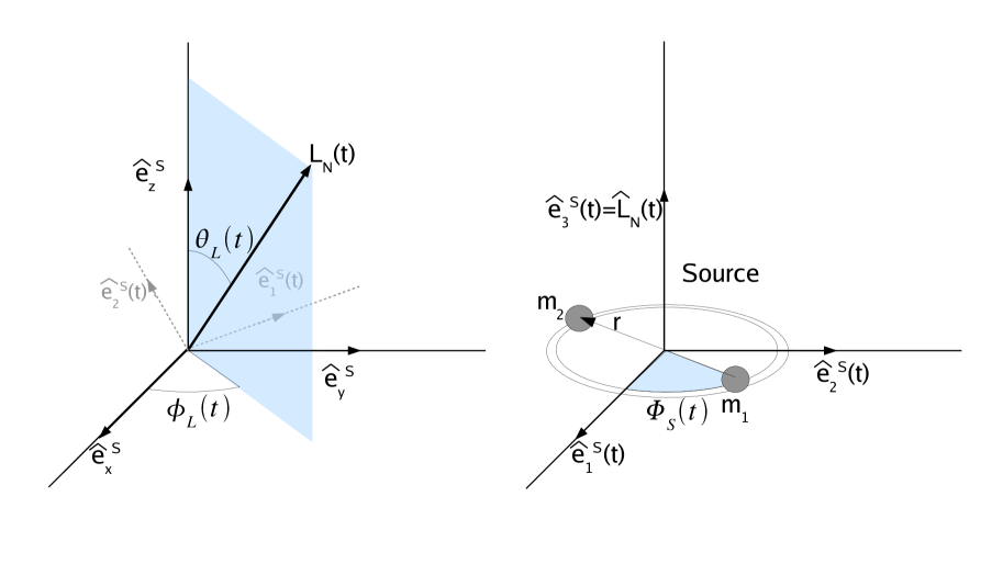
Figure 2.1: The binary in the source frame. The left hand plot shows the binary’s orbital angular momentum $\mbox{\boldmath$L$}_{N}$ within the fixed source frame $\{\mbox{\boldmath$e$}_{x}^{S},\mbox{\boldmath$e$}_{y}^{S},\mbox{\boldmath$e$}_{z}^{S}\}$. We also show the orthonormal basis for the instantaneous orbital plane $\{\mbox{\boldmath$e$}_{1}^{S},\mbox{\boldmath$e$}_{2}^{S}\}$. The right hand plot shows the binary within the orthonormal basis $\{\mbox{\boldmath$e$}_{1}^{S},\mbox{\boldmath$e$}_{2}^{S}\}$. The separation vector of the binary’s components $r$ and the orbital phase $\Phi_{S}$ are marked on this plot.

In order to project the quadrupolar moment $Q$ of the system onto the detector we use the tensor $P$ as shown in Eq. (2.15). We will define the (fixed) radiation source frame relative to our previously defined fixed source frame:

$$\mbox{\boldmath$e$}_{x}^{R} = \mbox{\boldmath$e$}_{x}^{S}\cos\Phi-\mbox{\boldmath$e$}_{z}^{S}\sin\Phi$$ (2.21)

$$\mbox{\boldmath$e$}_{y}^{R} = \mbox{\boldmath$e$}_{y}^{S}$$ (2.22)

$$\mbox{\boldmath$e$}_{z}^{R} = \mbox{\boldmath$e$}_{x}^{S}\sin\Phi+\mbox{\boldmath$e$}_{z}^{S}\cos\Phi$$ (2.23)

where the $\Phi$ is the angle between the vector $N$ which points from the source to the detector and $\mbox{\boldmath$e$}_{z}^{S}$. Similarly to how we defined $\{\mbox{\boldmath$e$}_{+}^{S},\mbox{\boldmath$e$}_{\times}^{S}\}$ we also define polarization tensors of the radiation frame (following the notation of BCV2 [40]):

$$\mbox{\boldmath$T$}_{+}\equiv\mbox{\boldmath$e$}_{x}^{R}\otimes\mbox{\boldmath$e$}_{x}^{R}-\mbox{\boldmath$e$}_{y}^{R}\otimes\mbox{\boldmath$e$}_{y}^{R},\;\,\,\,\mbox{\boldmath$T$}_{\times}\equiv\mbox{\boldmath$e$}_{x}^{R}\otimes\mbox{\boldmath$e$}_{y}^{R}+\mbox{\boldmath$e$}_{y}^{R}\otimes\mbox{\boldmath$e$}_{x}^{R}.$$ (2.24)

We also define the detector frame $\{\overline{\mbox{\boldmath$e$}}_{x},\overline{\mbox{\boldmath$e$}}_{y},\overline{\mbox{\boldmath$e$}}_{z}\}$ so that the detector’s arms lie along $\overline{\mbox{\boldmath$e$}}_{x}$ and $\overline{\mbox{\boldmath$e$}}_{y}$. The radiation and detection frames are shown in Fig. 2.2.

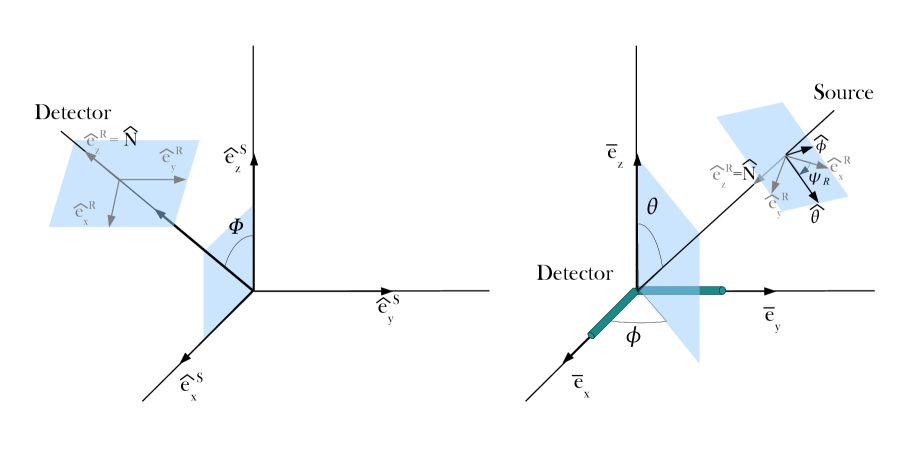
Figure 2.2: The radiation and detector frames. The left hand plot shows the fixed radiation frame $\{\mbox{\boldmath$e$}_{x}^{R},\mbox{\boldmath$e$}_{y}^{R},\mbox{\boldmath$e$}_{z}^{R}\}$ and the fixed source frame $\{\mbox{\boldmath$e$}_{x}^{S},\mbox{\boldmath$e$}_{y}^{S},\mbox{\boldmath$e$}_{z}^{S}\}$. We choose $\mbox{\boldmath$e$}_{z}^{R}$ to lie along the vector $N$ which points from the source to the detector. The right hand plot shows the detector in the frame $\{\overline{\mbox{\boldmath$e$}}_{x},\overline{\mbox{\boldmath$e$}}_{y},\overline{\mbox{\boldmath$e$}}_{z}\}$ chosen so that the detector’s arms lie along $\overline{\mbox{\boldmath$e$}}_{x}$ and $\overline{\mbox{\boldmath$e$}}_{y}$.

The tensor $P$ will depend upon the sky position $(\theta,\phi)$ and polarization angle $\psi_{P}$ of the source in relation to the detector. The inclination angle $\iota$ of a binary system is the angle between the vector $N$ joining the binary and detector, and the binary’s orbital angular momentum $L$,

$$\iota=\cos^{-1}\hat{\mbox{\boldmath$L$}}\cdot\hat{\mbox{\boldmath$N$}}.$$ (2.25)

A circular orbit with inclination angle $\iota\neq 0,\pi$ will make an ellipse on the plane of the sky (i.e., the plane containing $\mbox{\boldmath$e$}_{x}^{R}$ and $\mbox{\boldmath$e$}_{y}^{R}$ ). The orientation of this ellipse is described by the polarization angle $\psi_{P}$. For a binary consisting of spinning components, both inclination $\iota$ and the polarization angle $\psi_{P}$ will be functions of time due to the precession of the orbital plane. Using the FC style convention, the polarization angle $\psi_{P}$ is measured anti-clockwise from the semi-major axis of the ellipse made by projecting the binary’s orbit onto the plane of the sky to a line of constant azimuth $\hat{\theta}$ (i.e., a vertical line from the detector’s horizon). This is shown in Fig. 2.3. Note that there are two parts of the polarization angle shown on this figure; i) $\psi_{R}$ is the (constant) angle between the x-axis of the radiation frame $\mbox{\boldmath$e$}_{x}^{R}$ and $\hat{\theta}$ and ii) $\psi_{t}(t)$ which is the angle between the semi-major axis of the ellipse made by projecting the binary’s orbit onto the plane of the sky and $\mbox{\boldmath$e$}_{x}^{R}$ which will evolve as the binary precesses.

Note that during the relatively short duration of the inspiral we can make the approximation that the sky position $(\theta,\phi)$ of the source is constant. For sources that emit for longer duration in the detectors band of good sensitivity, such as pulsars that will be observed by LIGO or inspiral events that will be observed by LISA, it is necessary to include the time-dependence of the source’s sky position when calculating the detector’s response.

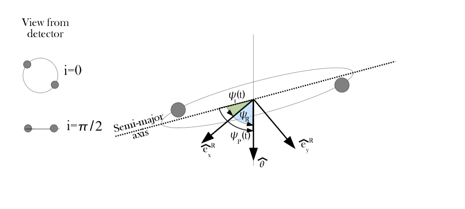
Figure 2.3: The two small diagrams on the left show projections of a circular orbit onto the plane of the sky with inclination angle $\iota=0$ and $\iota=\pi/2$. The diagram on the right shows the polarization angle $\psi_{P}(t)$ measured anti-clockwise from the semi-major axis of the ellipse made by projecting the binary’s orbit onto the plane of the sky to a line of constant azimuth $\hat{\theta}$ (i.e., a vertical line from the detector’s horizon). We see that $\psi_{P}(t)$ is the sum of the angles $\psi_{t}(t)$ measured between the semi-major axis and $\mbox{\boldmath$e$}_{x}^{R}$ and $\psi_{R}$ measured between $\mbox{\boldmath$e$}_{x}^{R}$ and $\hat{\theta}$. Since the radiation frame is fixed, $\psi_{R}$ remains constant with time. As the binary precesses $\psi_{t}(t)$, and therefore $\psi_{P}(t)$, will evolve.

The antenna patterns $F_{+}$ and $F_{\times}$ encode the detector’s directional sensitivity to plus ($+$) and cross ($\times$) polarization gravitational waves (see, for example Eqs. (4a,b) of ACST [12] or Eqs. (29) and (30) of BCV2 [40]) and are given by

$$F_{+}(t)=\frac{1}{2}\left(1+\cos^{2}\theta\right)\cos 2\phi\cos 2\psi_{R}-\cos\theta\sin\phi\sin 2\psi_{R},$$ (2.26)

$$F_{\times}(t)=\frac{1}{2}\left(1+\cos^{2}\theta\right)\cos 2\phi\cos 2\psi_{R}+\cos\theta\sin\phi\sin 2\psi_{R}.$$ (2.27)

The final form for the detector response is

$$h_{\rm{resp}}=\frac{\mu}{D}\frac{M}{r}\underbrace{-2\left(\left[\mbox{\boldmath$e$}_{+}^{S}\right]^{ij}\cos 2\Phi_{S}+\left[\mbox{\boldmath$e$}_{\times}^{S}\right]^{ij}\sin 2\Phi_{S}\right)}_{\mbox{\boldmath$Q$}}\underbrace{-2\left(\left[\mbox{\boldmath$T$}_{+}\right]_{ij}F_{+}+\left[\mbox{\boldmath$T$}_{\times}\right]_{ij}F_{\times}\right)}_{\mbox{\boldmath$P$}}.$$ (2.28)

Note that $P$ does not vary with time and that the time evolution of the binary is encoded within $Q$.

2.2.4 Parameters of the binary

17 physical parameters are required to fully describe a generic spinning binary system relative to a particular observer. These parameters are the masses of the binary’s components, $m_{1}$ and $m_{2}$ (2); the spins of the binary’s components, $\mbox{\boldmath$S$}_{1}(t)$ and $\mbox{\boldmath$S$}_{2}(t)$ (6), the orbital angular momentum of the system, $\mbox{\boldmath$L$}_{N}(t)$ (3), and the orbital phase $\Phi_{S}(t)$ (1) at a particular time $t$; the eccentricity $e$ and the point of perihelion (or aphelion) (2) and the distance and direction of the observer from the system $N$ (3). Note that in this analysis we assume that the emission of gravitational waves has circularized the binary’s orbit before it is observable (see Sec. 2.2.1).

The set of parameters listed here is not unique since various parameters can be recoded in terms of other parameters with no loss of information. For instance specifying both component masses $m_{1}$ and $m_{2}$ is obviously equivalent to specifying both total mass $M=m_{1}+m_{2}$ and the symmetric mass ratio $\eta=m_{1}m_{2}/M^{2}$ or the reduced mass $\mu=m_{1}m_{2}/M$. The absolute separation of the binary’s components can be found using $r=(M/\omega^{2})^{1/3}$ (from Kepler’s third law in geometric units) where $\omega$ is the orbital frequency. The direction of the orbital angular momentum relative to the detector can be specified by the inclination angle $\iota$ and polarization angle $\psi_{P}$ and its magnitude is given by Eq. (2.13). We can write the spins as $\mbox{\boldmath$S$}_{i}=\chi_{i}m_{i}^{2}\hat{\mbox{\boldmath$S$}}_{i}$, where $\chi_{i}$ is a dimensionless parameter such that $0<\chi_{i}<1$ for compact objects.

The parameters used to describe the system relative to an observer can be classified into two groups: intrinsic and extrinsic parameters. Intrinsic parameters describe the system itself and include its masses and spins whereas the extrinsic parameters describe the system’s distance and orientation to an observer. This distinction proves significant in the design of the detection template families we use to search for spinning systems as it turns out that, in general, to determine intrinsic parameters we need to include them in the templates we use to matched-filter our detector data whereas extrinsic parameters can be found automatically by maximising over the matched-filter output.

2.3 Development of detection template families to capture gravitational waves from spinning systems

In the introduction (Sec. 1.4) we showed that the optimal method to detect a known signal in a noisy data stream is to perform matched-filtering using templates that accurately represent the signal weighted (in the frequency domain) by the power spectrum of the detector noise. We cannot use the target model waveform (described in Sec. 2.2) as a detection template since the large number of parameters needed to describe the waveform (i.e., 17, or 15 if we assume circular orbits) mean that we would require an intractably huge number of templates to cover the parameter space (i.e., the range of masses, spin magnitudes and orientations) we wish to search.

Detection template families

Instead of using the target model, we will make use of a detection template family (DTF) that is designed to capture the essential features of the true gravitational wave signal (as approximated by the target model) but which depends on a smaller number of parameters. Detection templates might be parameterised by either physical parameters of the source or, as in the case of the DTF we will use, by non-physical or phenomenological parameters that describe the properties of the observed waveform rather than the source itself.

At their best, DTFs can reduce the computational requirements of a gravitational wave search while achieving essentially the same detection performance as exact templates (i.e., as generated using the target model). However, DTFs can include non-physical signal shapes that may increase the number of spurious triggers caused by noise (i.e., false alarms) which will in turn require us to set larger SNR thresholds and will affect the calculation of upper limits (see Sec. 2.8). Detection template families are also less adequate for parameter estimation, since the mapping between the detection template parameters and those of the binary are not one-to-one, this is why they are called detection template families.

Apostolatos (1995) [10] introduces the fitting factor ($FF$) as a quantitative measure of how well a given family of templates can “fit” a predicted gravitational waveform. The value of the fitting factor gives the reduction in signal to noise ratio (SNR) caused by using a given template family rather than the true signal, this is described in more detail in the next few Sections. In the terminology of Damour et al. (2001) [53]) we would say that DTFs are effectual (good fitting factor with target model) if not particularly faithful (i.e., poor estimation of parameters of target model).

The distance-range of a search for gravitational wave signals emitted by astrophysical systems is limited by the lowest SNR for which a true signal can be distinguished from noise. Using a detection template family with a $FF=0.9$ would result in a $10\%$ drop in distance-range and a corresponding $(1-0.9^{3}\approx)27\%$ drop in detectable event rate when compared with using “perfect” templates with $FF=1$. Apostolatos measures low fitting factors when using non-modulated PN templates to search for spin-modulated gravitational wave signals (Sec. VIII of Apostolatos (1995) [10]. Results from this analysis will be discussed later in this Section). These results clearly motivate the development of a detection template family which can accurately model the spin-induced modulation of the gravitational wave signal. We will now review the analysis of the effects of precessing, inspiraling binary systems and see how this has informed the development of a new detection template family designed to capture their gravitational wave emission.

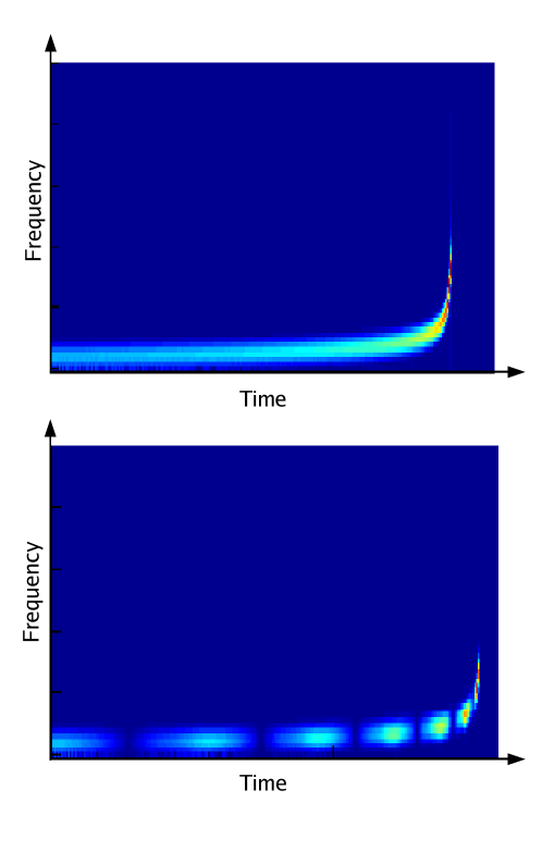
Figure 2.5: Spectrograms showing the gravitational waveforms we expect to observe from the late inspiral phase of two different binary systems, one consisting of non-spinning bodies (upper plot) and the other consisting of maximally spinning bodies (lower plot). Both systems are in quasi-circular orbits (i.e., not eccentric, although the binary with spinning components will precess) and are identical apart from the spin of their component bodies. The spin-induced precession of the binary’s orbital plane causes modulation of the gravitational wave signal and can be clearly seen in the lower spectrogram. The motion of LISA will cause similar modulations in the gravitational waves it will observe.

2.3.1 Previous analysis on the effect of spin on gravitational waves

In ACST [12] the authors consider a simplified form of the target model which neglects other post-Newtonian corrections in order to emphasise the effects of spin upon upon the system’s dynamics and gravitational wave emission. The authors concentrate their analysis on two special binary configurations; i) $m_{1}\simeq m_{2}$ which could represent a NS-NS system or a symmetric BH-BH system and ii) $\mbox{\boldmath$S$}_{2}=0$ which could represent a very asymmetric system ($m_{1}\gg m_{2}$) for which the spin of the lower mass component could be neglected. For case i) the authors make the additional assumption that spin-spin effects can be ignored since they occur at a higher post-Newtonian order (2PN), and are therefore typically smaller than the leading spin-orbit term (1.5PN). Spin-spin effects are not present for a system with only one spinning component as in case ii). Making the assumptions described the authors were able to write the equations governing the system’s precession as

$$\dot{\hat{\mbox{\boldmath$S$}}}_{1} = \left(2+\frac{3m_{2}}{2m_{1}}\right)\frac{\mbox{\boldmath$J$}}{r^{3}}\times\hat{\mbox{\boldmath$S$}}_{1}$$ (2.29)

$$\dot{\hat{\mbox{\boldmath$L$}}}_{N} = \left(2+\frac{3m_{2}}{2m_{1}}\right)\frac{\mbox{\boldmath$J$}}{r^{3}}\times\hat{\mbox{\boldmath$L$}}_{N}$$ (2.30)

where $\mbox{\boldmath$J$}=\mbox{\boldmath$L$}+\mbox{\boldmath$S$}$ and $\mbox{\boldmath$S$}=\mbox{\boldmath$S$}_{1}+\mbox{\boldmath$S$}_{2}$ . For these ACST configurations the authors constructed approximate solutions to the precession and inspiral equations and were able to gain insight into the dynamics of these binaries during their inspiral.

The authors identify two distinct evolutionary behaviours of the binary: i) simple precession occurs when total angular momentum $\mbox{\boldmath$J$}>0$ and the orbital angular momentum $\mbox{\boldmath$L$}_{N}$ and the spin angular momentum $S$ precess about a near constant $J$, ii) transitional precession occurs when $L$ and $S$ are anti-aligned and of the same approximate magnitude such that $\mbox{\boldmath$J$}\sim 0$ and the system temporarily “loses its gyroscopic bearings and tumbles in space”. As discussed previously in Sec. 2.2.2, $|\mbox{\boldmath$S$}|$ will remain almost constant during the course of inspiral while $|\mbox{\boldmath$L$}|$ will decay with time. Therefore, for transitional precession to occur we require that initially $|\mbox{\boldmath$L$}|>|\mbox{\boldmath$S$}|$ and that $L$ and $S$ be approximately anti-aligned with each other.

The evolution of orbital $L$, spin $S$ and total angular momentum $J$ during simple and transitional precessions is shown in Fig. 2.6. Considering the simplified precession equations (Eqs. (2.29) and (2.30)) we can show that $L$ and $S$ maintain fixed directions relative to each other as they precess about $J$. We can write

$$\kappa\equiv\hat{\mbox{\boldmath$S$}}\cdot\hat{\mbox{\boldmath$L$}}$$ (2.31)

where $\kappa$, and therefore the opening angle $\rm{cos}^{-1}\kappa$ between $L$ and $S$, will remain constant throughout the inspiral . The decay of $|\mbox{\boldmath$L$}|$ and $|\mbox{\boldmath$J$}|$ during the inspiral as $|\mbox{\boldmath$S$}|$ remains approximately constant will cause the opening angle $\lambda_{L}$ between $L$ and $J$ to increase during the inspiral. This is shown in Fig. 2.6. The random nature of the motion of $J$ during transitional precession makes the accurate prediction of the resulting waveform practically impossible and it is therefore fortunate that most inspiral evolutions do not exhibit transitional precession (this is discussed further in Sec. 2.3.2).

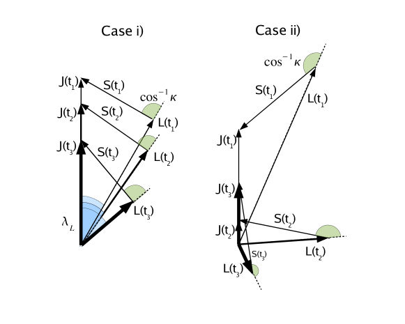
Figure 2.6: The evolution of orbital angular momentum $L$, spin angular momentum $S$ and total angular momentum $J$ during simple and transitional precession. In case i) only simple precession occurs as the total angular momentum $J$ remains relatively large and roughly constant in direction while $L$ and $S$ precess about it. In case ii) the evolution undergoes simple precession at early times ($t_{1}$) until at around $t_{2}$, $L$ has become anti-aligned with and similar in magnitude to $S$ so that $\mbox{\boldmath$J$}=\mbox{\boldmath$L$}+\mbox{\boldmath$S$}\sim 0$. The system will undergo a period of transitional precession, during which the system will tumble randomly in space, until $|\mbox{\boldmath$L$}|<|\mbox{\boldmath$S$}|$ and simple precession is resumed ($t_{3}$). This figure is based upon Fig. 2 of ACST [12].

From the simplified precession equations (Eqs. (2.29) and (2.30)) we see that during simple precession $L$ and $S$ will precess about $J$ with angular frequency

$$\Omega_{p}=\left(2+\frac{3m_{2}}{2m_{1}}\right)\frac{|\mbox{\boldmath$J$}|}{r^{3}}=\frac{d\alpha}{dt}$$ (2.32)

where we have also defined the precession angle $\alpha$ (see Fig. 2.7). The authors of ACST [12] considered cases where $|\mbox{\boldmath$L$}|\gg|\mbox{\boldmath$S$}|$ and where $|\mbox{\boldmath$S$}|\gg|\mbox{\boldmath$L$}|$ and found that the evolution of the precession angle could be approximated by a power law in orbital frequency $f=\omega/2\pi$:

$$\frac{\alpha(f)}{2\pi}\simeq\left\{\begin{array}[]{ll}11\left(1+\frac{3m_{2}}{4m_{1}}\right)\frac{10M_{\odot}}{M}\frac{10{\rm{Hz}}}{f}&\rm{for}\,|\mbox{\boldmath$L$}|\gg|\mbox{\boldmath$S$}|\\ 1.9\left(1+\frac{3m_{2}}{4m_{1}}\right)\frac{m_{1}}{m_{2}}\frac{S}{m_{1}^{2}}\left(\frac{10M_{\odot}}{M}\frac{10{\rm{Hz}}}{f}\right)^{2/3}&\rm{for}\,|\mbox{\boldmath$S$}|\gg|\mbox{\boldmath$L$}|.\end{array}\right.$$ (2.33)

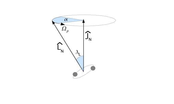
Figure 2.7: During simple precession the orbital angular momentum $L$ of the (ACST configuration) binary will precess about the total angular momentum $J$ with frequency $\Omega_{p}$. The opening angle $\lambda_{L}$ and the precession angle $\alpha$ are also identified. This figure is based upon Fig. 4 of ACST [12].

Apostolatos (1995) [10] introduces the fitting factor (FF) as a quantitative measure of the reduction in SNR caused by using a particular family of templates in order to capture a predicted gravitational waveform. The fitting factor is given as

$${\rm{FF}}={\rm{max}}_{\lambda_{1},\lambda_{2}\dots}\frac{\left<h,T_{\lambda_{1},\lambda_{2}\dots}\right>}{\sqrt{\left<h,h\right>\left<T_{\lambda_{1},\lambda_{2}\dots},T_{\lambda_{1},\lambda_{2}\dots}\right>}}$$ (2.34)

where $h$ is our best prediction of the gravitational waveform that will be observed and $T$ is a template designed to capture $h$ and which is parameterised by $\lambda_{1},\lambda_{2}\dots$. The denominator ensures that $0\leq{\rm{FF}}\leq 1$. Apostolatos (1995) [10] writes the detector response to a precessing, inspiraling binary as

$$\tilde{h}_{\rm{resp}}(f)\simeq\frac{1}{2}\tilde{h}_{C}(f)\times{\rm{AM}}\times{\rm{PM}}$$ (2.35)

where $\tilde{h}_{C}(f)$ is a non-modulated carrier signal and AM and PM represent amplitude and phase modulations caused by spin-induced precession (see Eq. (17) of Apostolatos (1995) [10] and note that the final multiplicative factor is approximately unity). Apostolatos investigates the relative influence of phase and amplitude modulations upon the fitting factor when the templates used to detect spin-modulated gravitational waves do not themselves include the effects of spin. It was found that at worst, amplitude modulation alone can only account for fitting factors dropping to $\sim 0.9$ whereas phase modulation can cause the fitting factor to drop below $0.6$.

Apostolatos also investigated the effect of the opening angle between spin and orbital angular momentum (i.e., $\cos^{-1}\kappa$) on the fitting factors. When considering a maximally spinning $10M_{\odot}$ BH and a non-spinning NS, $FF<0.9$ were measured for around a quarter of systems with a $\cos^{-1}\kappa=30^{\circ}$. When the opening angle is increased to $\cos^{-1}\kappa=140^{\circ}$ then $FF<0.9$ are measured for nearly all systems.

Building on work in ACST [12], Apostolatos suggests in Refs. [10, 11] that the spin-induced modulational effects of the gravitational wave signal’s phase could be captured by adding modulational terms to the standard non-modulational (NM) frequency domain phasing of templates used to search for the inspiral of binaries with non-spinning components (see Eq. (12) of Apostolatos (1996)) [11]):

$$\psi_{\rm{Spin-Modulated}}(f)\rightarrow\psi_{\rm{Non-Modulated}}(f)+\mathcal{C}\cos(\delta+\mathcal{B}f^{-2/3}).$$ (2.36)

This is the Apostolatos ansatz. It makes sense that the modulational term occurs at $f^{-2/3}$ since this corresponds to the power law evolution of the precession angle when $|\mbox{\boldmath$S$}|\gg|\mbox{\boldmath$L$}|$ (see Eq. (2.33)). An implementation of this detection template family (which we shall refer to as the Apostolatos family) was tested in Grandclément et al. (2003) [76]. Although the fitting factor increased by around $15-30\%$ compared to using templates with no spin-modulation included, the fitting factors were still only $\sim 0.7$ which would lead to a drop in expected event rate of up to $80\%$. We will now describe the work of Buonanno, Chen and Vallisneri which led to the development of a detection template family which captures spin-modulated gravitational waves with $FF>0.9$ and which we shall use to search for gravitational waveforms in real LIGO data.

2.3.2 BCV2 analysis of spinning binary systems

In BCV2 the authors used the target model described in Sec. 2.2 to further investigate the effects of spin upon the observed gravitational waveform which led to the development of a new detection family (which we shall refer to as the BCV2 DTF). The BCV2 analysis considers a wider range of systems than ACST and do not limit themselves the ACST configurations previously discussed (i.e., either $m_{1}\simeq m_{2}$ or $\mbox{\boldmath$S$}_{2}=0$). In BCV2 the authors consider BH-BH systems with masses $(20,10)M_{\odot}$, $(15,15)M_{\odot}$, $(20,5)M_{\odot}$, $(10,10)M_{\odot}$ and $(7,5)M_{\odot}$ consisting of maximally spinning BHs and NS-BH systems with masses $(1.4,10)M_{\odot}$ consisting of a maximally spinning BH and a non-spinning NS (Sec VIB and VIC of BCV2 [40]) . We shall refer to these as BCV2 configurations. The choices of spin are not based upon astrophysical results (most of the spin measurements summarised earlier were published after BCV2 [40]) but to emphasise the effects of spins upon the evolution and emission of these systems. We summarise the findings of their analysis here.

When ignoring spin-spin coupling (but still considering binaries consisting of two spinning bodies) the authors of BCV2 [40] find a generalisation of Eq. (2.31) for the opening angle between the orbital angular momentum and the spins:

$$\kappa_{\rm{eff}}\equiv\frac{\hat{\mbox{\boldmath$L$}}_{N}\cdot\mbox{\boldmath$S$}_{{\rm{eff}}}}{M^{2}}$$ (2.37)

where we have defined an effective spin

$$\mbox{\boldmath$S$}_{{\rm{eff}}}\equiv\left(1+\frac{3m_{2}}{4m_{1}}\right)\mbox{\boldmath$S$}_{1}+\left(1+\frac{3m_{1}}{4m_{2}}\right)\mbox{\boldmath$S$}_{2}.$$ (2.38)

The authors of BCV2 [40] investigate the regularity that transitional precession occurs. For transitional precession to be observed, we require that $|\mbox{\boldmath$L$}_{N}|=|\mbox{\boldmath$S$}|\leq|\mbox{\boldmath$S$}_{1}|+|\mbox{\boldmath$S$}_{2}|$ before the system plunges, i.e., $f_{\rm{trans}}^{\rm{min}}<f_{\rm{Schw}}$ where we assume that plunge occurs at the Schwarzschild radius. For transitional precession to be observed, they find that the symmetric mass ratio must be less than some limiting value $\eta\lesssim 0.22$, see Sec. IIIE of BCV2 [40] . Of the BCV2 configuration binaries considered, only the $(20,10)M_{\odot}$, $(20,5)M_{\odot}$ and $(10,1.4)M_{\odot}$ binaries satisfy the condition on $\eta$. The authors of BCV2 [40] considered $\geq 200$ initial configurations of each of these binaries and observed no transitional precession of the $(20,10)M_{\odot}$ and $(10,1.4)M_{\odot}$ binaries and only a few cases of transitional precession of the $(20,5)M_{\odot}$ binary. Indeed, for the $(10,1.4)M_{\odot}$ binary, consisting of a maximally spinning BH and a non-spinning NS, the magnitude of the spin angular momentum was always greater than the magnitude of the orbital angular momentum meaning that transitional precession could never occur for any configuration of the binaries spin and orbital angular momentum.

The authors of BCV2 [40] also investigated the effects of the spin terms on the evolution of the orbital angular frequency $\omega$ (Eqs. (2.3), (2.5) and (2.6)) and on the accumulated orbital phase $\Psi$ (Eq. 2.10). They find that the effects of spin on the accumulated orbital phase $\Psi$ would be largely non-modulational and could be well captured by the phasing used to describe binaries with non-spinning components. It is important to acknowledge that although the accumulated orbital phase $\Psi$ is not modulated by the effects of spin, the phase (and amplitude) of the gravitational waveform observed at the detector will be modulated by the spin-induced precession of the orbital plane and that these effects should not be neglected. The phase $\Phi_{S}(t)$ which enters the general expression for detector response $h_{\rm{resp}}$ (see Eq. (2.28)) is measured with respect to basis vector $\mbox{\boldmath$e$}_{1}^{S}$ which is always in the instantaneous orbital plane (i.e., $\mbox{\boldmath$L$}_{N}(t)\cdot\mbox{\boldmath$e$}_{1}^{S}(t)=0$, see Fig. 2.1). In general, $\Phi(t)\neq\Psi(t)$ since $\mbox{\boldmath$e$}_{1}^{S}$ (and also $\mbox{\boldmath$e$}_{2}^{S}$) can have arbitrary rotation about $\mbox{\boldmath$L$}_{N}$. In BCV2 [40] the authors define a new precessing convention for the basis $\{\mbox{\boldmath$e$}_{1}^{S},\mbox{\boldmath$e$}_{2}^{S}\}$ such that $\Phi(t)=\Psi(t)$ which allows the use of $\Psi(f)$ when we write down the detector response $h_{\rm{resp}}$. From their earlier observations we know that the non-modulational phase $\psi_{\rm{NM}}(f)$ used to describe the phasing of binaries with non-spinning components is a good approximation to $\Psi$.

2.4 The BCV2 detection template family for spinning systems

Following their analysis the authors of BCV2 [40] proposed a detection template family representing a generalisation of the Apostolatos ansatz designed to capture gravitational waveforms from precessing, inspiraling binaries in the adiabatic limit. Significantly we will find in Sec. 2.4.1 that the majority of the parameters of this DTF are extrinsic parameters that can be found in a computationally cheap manner by maximisation of the measured SNR. From BCV2 [40] Eq. (86) we write the form if the DTF:

$$h(\dots;f)=\left[\sum_{k=1}^{n}(\alpha_{k}+i\alpha_{k+n})\mathcal{A}_{k}(f)\right]e^{2\pi ift_{0}}e^{i\psi_{\rm{NM}}(f)}$$ (2.39)

for $f>0$ and $h(f)=h^{*}(-f)$ for $f<0$. The $\alpha$’s represent the global phase, the strength of the amplitude modulation due to spin-induced precession, the relative phase of these modulations to the leading order amplitude ($f^{-7/6}$) and the internal complex phase of the modulation [40]. The (real) amplitude functions $\mathcal{A}_{k}$ depend on the precise form of the template chosen. The function $\psi_{\rm{NM}}$ is the non-modulated phasing of a non-spinning binary and is given as power series of gravitational wave frequency $f$:

$$\psi_{\rm{NM}}(f)=f^{-5/3}\left(\psi_{0}+\psi_{1}f^{1/3}+\psi_{2}f^{2/3}+\psi_{3}f\dots\right).$$ (2.40)

We have discussed in Sec. 2.3.2 that the non-modulated phase $\psi_{\rm{NM}}$ used to describe a binary with non-spinning components has been to capture well the accumulated orbital phase of binaries with spinning components. In practice we find that the phasing of the gravitational wave can be captured well using only the $\psi_{0}$ and $\psi_{3}$ terms and we will neglect the other terms in this expansion .

In BCV2 [40] the authors suggest and test three forms of the detection template family before recommending the third family which they refer to as $(\psi_{0},\psi_{3},\beta)_{6}$ (Eq. (90) of BCV2 [40]):

$$(\psi_{0}\psi_{3}\beta)_{6}:$$

$$h(\dots;f) = f^{-7/6}\big{[}(\alpha_{1}+i\alpha_{2})+(\alpha_{3}+i\alpha_{4})\cos(\beta f^{-2/3})$$ (2.41)

$$+ (\alpha_{5}+i\alpha_{6)})\sin(\beta f^{-2/3})\big{]}$$

$$\theta(f_{\rm{cut}}-f)e^{2\pi ift_{0}}\,\rm{exp}\,i\big{[}\psi_{0}f^{-5/3}+\psi_{3}f^{-2/3}\big{]}.$$

Rewriting Eq. (2.4) similarly to Eq. (2.39) we find the three real amplitude functions, $\mathcal{A}_{k}(f_{\rm{cut}},\beta;f)$ of $(\psi_{0},\psi_{3},\beta)_{6}$ to be

$$\mathcal{A}_{1}(f_{\rm{cut}},\beta;f) = f^{-7/6}\theta(f_{\rm{cut}}-f)$$

$$\mathcal{A}_{2}(f_{\rm{cut}},\beta;f) = f^{-7/6}\cos(\beta f^{-2/3})\theta(f_{\rm{cut}}-f)$$

$$\mathcal{A}_{3}(f_{\rm{cut}},\beta;f) = f^{-7/6}\sin(\beta f^{-2/3})\theta(f_{\rm{cut}}-f).$$ (2.42)

The $\beta$ parameter varies to capture the effects of spin modulation. We see that in the Apostolatos ansatz Eq. (2.36), the term $\cos(\beta f^{-2/3})$ is an approximation for the precession angle $\alpha$ when $|\mbox{\boldmath$S$}|\gg|\mbox{\boldmath$L$}|$ (see Eq. (2.33)). The parameter $\beta$ takes a similar role in this DTF. In Buonanno et al. (2005) [37] (known as PBCVT) the authors provide some physical interpretation of the $\beta$ parameter identifying it as representing the rate of change of the precession angle $\alpha$, i.e., $\Omega_{p}=d\alpha/dt$ at the frequency band of good detector sensitivity.

The function $\theta$ is the Heaviside step function which is defined as

$$\theta(x)=\left\{\begin{array}[]{cl}0&x<0\\ 1&x\geq 0\end{array}\right.$$

The parameter $f_{\rm{cut}}$ is used to terminate the template when we no longer have confidence that the template will provide a good match to the signal (i.e., at the late stages of inspiral when the adiabatic approximation is no longer valid). For gravitational wave frequency $f\leq f_{\rm{cut}}$ then $\theta(f_{\rm{cut}}-f)=1$. The choice of $f_{\rm{cut}}$ for our templates is discussed in Sec. 2.5.2.

Buonanno, Chen and Vallisneri measured the fitting factor of this detection template family and their results are presented in Sec. VIC of BCV2 [40] (see Fig. 11 in particular) . The BCV2 DTF described here $(\psi_{0},\psi_{3},\beta)_{6}$ outperforms the other variants of the DTF they considered, $(\psi_{0},\psi_{3},\beta)_{4}$ and $(\psi_{0},\psi_{3})_{2}$, which have fewer $\alpha$ terms and therefore less degrees of freedom with which to maximise their overlap with a given target waveform. The BCV2 DTF also outperformed the standard (physically parameterised) stationary phase approximation templates. Average fitting factors of $\simeq 0.93$ were measured for the NS-BH binaries and even higher $\geq 0.97$ for the BH-BH binaries considered (i.e., the BCV2 configurations discussed in Sec. 2.3.2). Lower fitting factors for the asymmetric systems (e.g., $(1.4,10)M_{\odot}$ NS-BH binaries) is unsurprising since we expect spin modulation to have most effect on these systems thereby making their waveforms more complicated and thus harder to capture accurately.

2.4.1 Maximisation of overlap over extrinsic parameters

When listing the parameters used to describe a binary system consisting of spinning components we divided the parameters into two categories: intrinsic parameters which describe properties of the system itself (e.g., masses, spins) and extrinsic parameters which describe the observers relation to the system (e.g., amplitude of observed emission, inclination and polarization angle). Now considering the problem of finding the template $h$ within our DTF (as given in Eq. (2.39)) which yields the highest overlap with a given target signal $s$, we find that we can usefully separate the parameters used to describe our templates into these categories. For the extrinsic parameters used to describe the templates (e.g., $\psi_{0}$, $\psi_{3}$, $\beta$ and $f_{\rm{cut}}$) we must construct templates corresponding to each set of these parameters we wish to search for. Conversely, we are able to search automatically through the range of our intrinsic parameters (e.g., $t_{0}$ and $\alpha_{1\dots 6}$) for the values which yield the best overlap.

To begin with we will consider the maximisation of the overlap over time. The overlap between a time-shifted template $h(t-t_{0})$ and a signal $s$ is given by

$$\left<s,h(t-t_{0})\right>=4\Re\int_{0}^{\infty}\tilde{s}^{*}(f)\tilde{h}(f)e^{2\pi ift_{0}}\frac{df}{S_{n}(f)}.$$ (2.43)

Note that in the case of no time-shift ($t_{0}=0$) we re-obtain the formulae for the inner product given in Eq. (1.101). Rather than evaluate the overlap separately for every value of $t_{0}$ (in reality our time-series will be discretized so there will be a finite number of values) we can employ the inverse Fourier transform to evaluate all values of $t_{0}$ automatically. Finding the value of $t_{0}$ which maximises the overlap is simply a case of noting the time at which the maxima in the resulting overlap time series occurs. We use the computationally efficient Fast Fourier transform (FFT) to carry out forward and inverse Fourier transforms (see Sec. 5.3 and e.g., Chapter 12 of Ref. [120] for documentation of FFTs).

Now we shall consider the maximisation of the overlap over the $\alpha$ parameters. Consider a template characterised only by its extrinsic parameters $h(t_{0},\alpha_{k})$ which has been normalised such that the inner product $\left<h,h\right>=1$. The overlap between the template $h$ and the signal $s$ is

$$\max_{t_{0},\alpha_{k}}\left<s,h(t_{0},\alpha_{k})\right>.$$ (2.44)

We find it expedient to orthonormalise our amplitude functions $\left<\widehat{\mathcal{A}}_{i},\widehat{\mathcal{A}}_{j}\right>=\delta_{ij}$ and then define our basis templates as

$$\hat{h}_{k}(t_{0};f) = \widehat{\mathcal{A}}_{k}(f)e^{2\pi ift_{0}}e^{i\psi_{\rm{NM}}}$$

$$\hat{h}_{k+n}(t_{0};f) = i\widehat{\mathcal{A}}_{k}(f)e^{2\pi ift_{0}}e^{i\psi_{\rm{NM}}}.$$ (2.45)

The orthonormalisation of the amplitude functions, $\mathcal{A}\rightarrow\widehat{\mathcal{A}}$ is a lengthy procedure and is described in the Appendix, Sec. 5.2. We are able to write our original template $h$ in terms of our basis templates $\hat{h}_{k}$:

$$h(t_{0},\alpha_{k};f)=\sum_{k=1}^{2n}\hat{\alpha}_{k}\hat{h}_{k}.$$ (2.46)

The overlap between the template $h$ and a signal $s$ would be:

$$\max_{t_{0},\alpha_{k}}\left<s,h(t_{0},\alpha_{k})\right>=\max_{t_{0}}\max_{\hat{\alpha}_{k}}\sum_{k=1}^{2n}\hat{\alpha}_{k}\left<s,\hat{h}_{k}(t_{0})\right>.$$ (2.47)

We will require that our templates be normalised and find that this will lead to a constraint on the $\hat{\alpha}_{k}$ values

$$\left<h,h\right> = 1$$ (2.48)

$$= \sum_{k=1}^{2n}\left<\hat{\alpha}_{k}\hat{h}_{k},\hat{\alpha}_{k}\hat{h}_{k}\right>$$

$$= \sum_{k=1}^{2n}\hat{\alpha}_{k}^{2}\left<\hat{h}_{k},\hat{h}_{k}\right>$$

$$= \sum_{k=1}^{2n}\hat{\alpha}_{k}^{2}$$

where we have made use of the fact that since the amplitude functions $\widehat{\mathcal{A}}_{k}$ are orthonormal, the basis templates are each orthonormalised, $\left<\hat{h}_{i},\hat{h}_{j}\right>=\delta_{ij}$. We can find $\hat{\alpha}_{k}$ that maximise the overlap by employing the method of Lagrange multipliers

$$\Lambda=\sum_{k=1}^{2n}\hat{\alpha}_{k}\left<s,\hat{h}_{k}(t_{0})\right>-\lambda\left[\sum_{k=1}^{2n}\hat{\alpha}_{k}^{2}-1\right]$$ (2.49)

which leads to

$$\hat{\alpha}_{k}=\frac{\left<s,\hat{h}_{k}(t_{0})\right>}{\sqrt{\sum_{j=1}^{2n}\left<s,\hat{h}_{j}(t_{0})\right>^{2}}}.$$ (2.50)

Substituting Eq. (2.50) into Eq. (2.47) we find the overlap maximised over $\hat{\alpha}_{k}$

$$\max_{t_{0},\alpha_{k}}\left<s,h(t_{0},\alpha_{k})\right>=\sqrt{\sum_{j=1}^{2n}\left<s,\hat{h}_{j}(t_{0})\right>^{2}}.$$ (2.51)

In the case where the data to be filtered $x(t)$ contains both signal $s(t)$ and noise $n(t)$, i.e., $x(t)=n(t)+s(t)$ we can define the SNR as

$$\rho=\max_{t_{0},\alpha_{k}}\left<x,h(t_{0},\alpha_{k})\right>=\sqrt{\sum_{j=1}^{2n}\left<x,\hat{h}_{j}(t_{0})\right>^{2}}$$ (2.52)

The implementation of the SNR calculation including the maximisation over time and $\alpha$ parameters is described in the Appendix, Sec. 5.3.

2.4.2 Testing the detection template family

We have shown in Secs. 5.1.2 and 1.4.1 that when filtering data $x$ with a single template $h$:

• The output of filtering $\left<x,h\right>$ will be a Gaussian distributed variable if $x(t)$ is a Gaussian distributed variable.

• The expectation value of $\left<n,h\right>$ will be zero if $\overline{n(t)}=0$.

• The variance of $\left<n,h\right>$ will be unity if we use a normalised template such that $\left<h,h\right>=1$.

Therefore, for a Gaussian distributed variable $x$ with mean $0$ and variance $1$, i.e. $x\sim N(0,1)$ we expect that $\left<x,h\right>\sim N(0,1)$. Also, for a Gaussian distributed variable $x$ with mean $\mu$ and variance $\sigma^{2}$, i.e. $x\sim N(\mu,\sigma^{2})$ we have

$$\chi_{n}^{2}=\sum_{i=1}^{n}\frac{x_{i}^{2}-\mu_{i}}{\sigma_{i}^{2}}.$$ (2.53)

where $n$ is the number of degrees of freedom of the $\chi^{2}$ distribution. The $\chi_{n}^{2}$ has mean $n$ and variance $2n$.

From Eq. (2.52) we see that

$$\rho^{2}=\max_{t_{0},\alpha_{k}}\left<x,h(t_{0},\alpha_{k})\right>^{2}=\sum_{j=1}^{2n}\left<x,\hat{h}_{j}(t_{0})\right>^{2}.$$ (2.54)

For $x\sim N(0,1)$ we expect $\left<x,\hat{h}_{j}(t_{0})\right>\sim N(0,1)$ and therefore that $\rho^{2}\sim\chi_{2n}^{2}$ (using the range of $n$ used in the summation in this equation).

In general, when $\beta\neq 0$ we have 6 (non-zero) basis templates $\hat{h}_{j}$ and we would therefore expect $\rho^{2}\sim\chi_{6}^{2}$. When $\beta=0$ we find that the (orthonormalised) amplitude functions $\widehat{\mathcal{A}}_{2}$ and $\widehat{\mathcal{A}}_{3}$ become zero at all frequencies (see Eqs. (5.26), (5.41) and (LABEL:app_A3hat)). Consequently we find that 4 of the 6 basis templates $\hat{h}_{j}$ defined in Eq. (2.4.1) become zero at all frequencies. Therefore, we will expect that when $\beta=0$, $\rho^{2}\sim\chi_{2}^{2}$. Figure 2.8 shows histograms of $\rho^{2}$ measured using our detection template family (with $\beta=0$ and $\beta\neq 0$) when filtering Gaussian white noise with zero mean and unit standard deviation. The response of our templates is as we would expect.

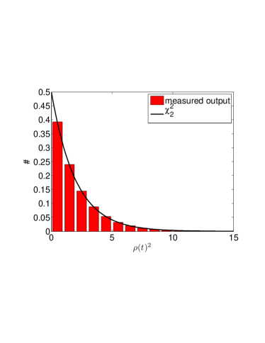
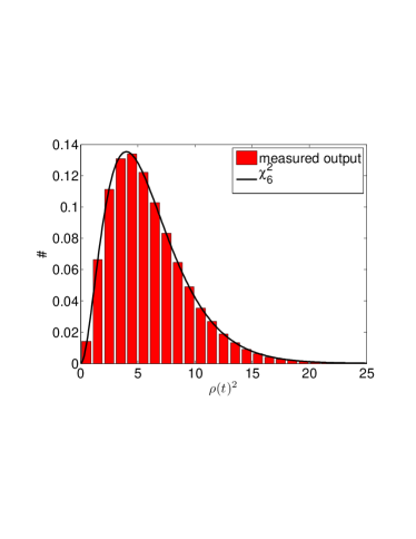
Figure 2.8: Histograms of $\rho^{2}$ when $\beta=0$ (left hand plot) and when $\beta\neq 0$ (right hand plot). As expected $\rho^{2}$ is distributed as a $\chi_{n}^{2}$ with the number of degrees of freedom $n$ equal to the number of non-zero basis templates $\hat{h}_{i}$ used to calculate $\rho^{2}$.

We also expect that for a normalised template $h$ that we would obtain an overlap of unity if we were to use a template as our input data i.e., $x=h$. Figure 2.9 shows the overlap measured (top plot) when we perform this test. As expected an overlap of unity was measured.

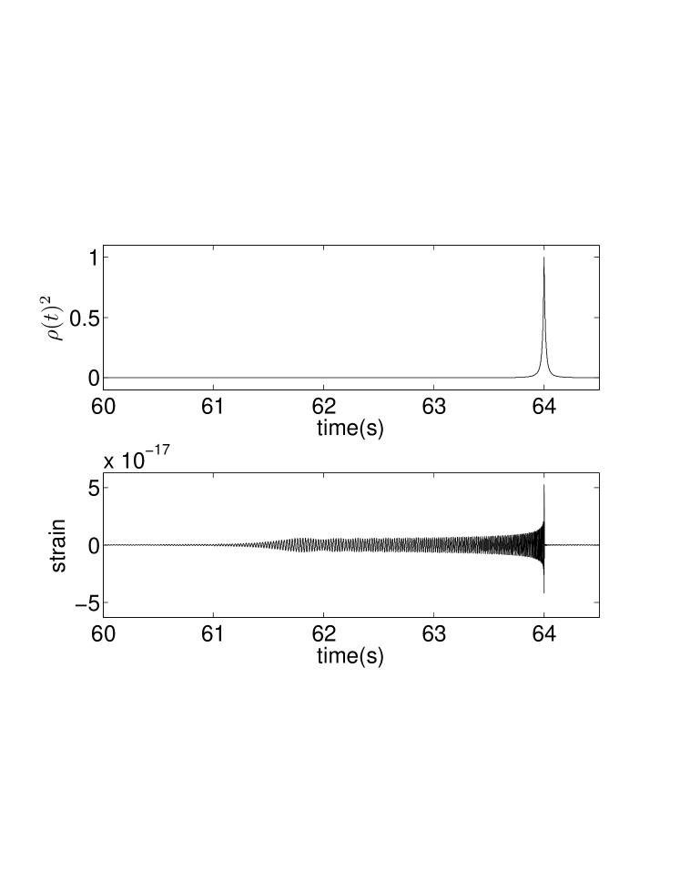
Figure 2.9: Plot showing the overlap ($\rho^{2}$) measured when filtering a template $h$ with itself. As expected we measure an overlap of unity at the end time of the waveform.

2.4.3 Estimating non-physical parameters in terms of physical parameters

We are able to construct approximate relationships between the physical parameters $M$, $\eta$ and $\chi$ of our spinning binary system and the non-physical parameters used in the detection template family $\psi_{0}$, $\psi_{3}$ and $\beta$. In Eq. (3.3) and (3.4) of Arun et al. (2005) [15] the phase of a gravitational wave inspiral is given to 3.5PN in the Fourier domain:

$$\psi(f) \equiv \Psi_{f}(t_{f})-\frac{\pi}{4}$$ (2.55)

$$= 2\pi ft_{c}-\phi_{c}-\frac{\pi}{4}+\frac{3}{128\eta\nu^{5}}\sum_{k=0}^{N}\alpha_{k}\nu^{k}$$

where $\nu=(\pi Mf)^{1/3}$, $M=m_{1}+m_{2}$ and $\eta=m_{1}m_{2}/M^{2}$. In BCV1 [41] (see Sec. VI) it was noted that the phasing of the target model could be captured well using only the $\psi_{0}$ and $\psi_{3}$ terms in the expansion of the non-modulational phase of the templates (see Eq. (2.40)) and setting the other $\psi$ coefficients equal to zero. The values of the $\alpha$ coefficients in Eq. (2.55) corresponding to the same order in frequency as $\psi_{0}$ and $\psi_{3}$ are $\alpha_{0}=1$ and $\alpha_{3}=-16\pi$ respectively. Equating the terms of Eq. (2.55) with the $\psi_{0}$ and $\psi_{3}$ terms of Eq. (2.40) corresponding to the same order in frequency we find

$$\psi_{0} = \frac{3}{128}\frac{1}{\eta(\pi M)^{5/3}}$$ (2.56)

$$\psi_{3} = -\frac{3}{8}\frac{\pi^{1/3}}{\eta M^{2/3}}.$$ (2.57)

From ACST [12] we find that the evolution of the precessional angle $\alpha_{p}$ can be approximated by power laws of $f$ in 2 extreme cases; $|\mbox{\boldmath$L$}|\gg|\mbox{\boldmath$S$}|$ and $|\mbox{\boldmath$S$}|\gg|\mbox{\boldmath$L$}|$. The first case, when $|\mbox{\boldmath$L$}|\gg|\mbox{\boldmath$S$}|$, corresponds to a binary with either comparable masses or which is at the early stages of inspiral (i.e., large separation). The second case, $|\mbox{\boldmath$S$}|\gg|\mbox{\boldmath$L$}|$, corresponds to a binary with small mass ratio (i.e., large mass asymmetry) or which is at the late stages of inspiral (i.e., small separation) [37]. In Fig. (3) of [91], Kidder shows the evolution of $|\mbox{\boldmath$L$}|$ and $|\mbox{\boldmath$S$}|$ with separation $r$ for both an equal mass binary and a binary with a small mass ratio. This figure effectively illustrates the regimes during which the two extreme cases $|\mbox{\boldmath$L$}|\gg|\mbox{\boldmath$S$}|$ and $|\mbox{\boldmath$S$}|\gg|\mbox{\boldmath$L$}|$ are relevant.

When $|\mbox{\boldmath$S$}|\gg|\mbox{\boldmath$L$}|$ we find .

$$\alpha_{p}(f)\sim 3.8\pi\left(1+\frac{3}{4}\frac{m_{2}}{m_{1}}\right)\frac{m_{1}}{m_{2}}\chi\left(\frac{10M_{\odot}}{M}\frac{10Hz}{f}\right)^{2/3}.$$ (2.58)

We use the parameter $\beta$ as the coefficient in the power law, $\alpha_{p}(f)=\beta f^{-2/3}$ and thus find that

$$\beta\propto\left(1+\frac{3}{4}\frac{m_{2}}{m_{1}}\right)\frac{m_{1}}{m_{2}}\chi\left(\frac{10M_{\odot}}{M}\right)^{2/3}.$$ (2.59)

In the analysis of [12] the authors assume either that $m_{1}=m_{2}$ (meaning that spin-spin coupling can be ignored) or that $\mbox{\boldmath$S$}_{2}=0$ which would correspond to systems with small mass ratio, e.g., the inspiral of a NS into a spinning BH. Asymmetric mass systems $m_{1}\gg m_{2}$ can be modelled as systems with only a single body spinning since even if both systems were spinning maximally $|\mbox{\boldmath$S$}_{1}|\gg|\mbox{\boldmath$S$}_{2}|$. Maximal value of $\beta$ occurs when $\chi=1$.

Using the $f^{-2/3}$ power law approximation of $\alpha_{p}(f)$ is only expected to perform well matching binaries with $|\mbox{\boldmath$S$}|\gg|\mbox{\boldmath$L$}|$ but is shown to match well with systems with $|\mbox{\boldmath$L$}|\gg|\mbox{\boldmath$S$}|$ [40].

2.5 Creating template banks

The detection template formula Eq. (2.4) describes a continuous multi-dimensional manifold containing every possible waveform that this family can generate. We can also imagine another manifold containing every possible gravitational waveform we might observe from a binary with spinning components. The parameters used to describe the detection templates/signals act as the co-ordinates on these manifolds. Figure 2.10 shows the continuous manifolds of signals and templates. We must now select a finite, discretely spaced subset of points on the continuous detection template manifold which will form the bank of templates we shall use to search for gravitational wave signals from binaries with spinning components. There are two important decisions to be made in choosing the templates for our bank: i) we must choose the parameter space we would like our template bank to cover (i.e., the range of masses and spins of our target waveforms we are interested in capturing) and ii) the spacing of the templates within this region of parameter space which will in turn directly influence the number of templates we will have in our bank and the computational cost of the search. We wish to space our templates as sparsely as possible (in order to minimize the computational cost of the search) while also ensuring that we will achieve good matches for any point on the continuous detection template manifold with one of the templates in the bank. We will consider the question of template spacing and placement first.

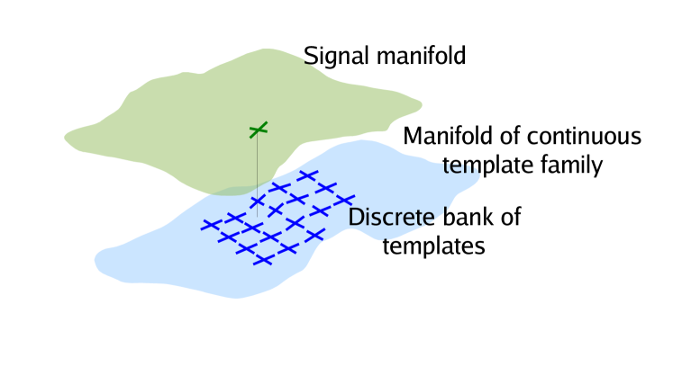
Figure 2.10: Schematic representation of the signal and continuous detection template family manifolds as 2 dimensional surfaces. The signal manifold (green) contains all the possible gravitational waveforms we might observe from a binary with spinning components. The continuous detection template family manifold (blue) contains all the waveforms that can be represented by our detection template family Eq. (2.4). We use the metric (of the intrinsic parameters, Eq. (2.62)) on the continuous detection template family in order to choose a finite set of templates (blue crosses) which we refer to as our template bank. We place the templates of our bank such that for any point chosen within the region of the continuous detection template family manifold we wish to cover, an overlap (or match) greater than the specified minimal match will be obtained with one of the templates in the bank. The fitting factor (previously discussed) describes the separation of the signal and template manifolds. If the fitting factor was unity for a region of parameter space the manifolds would be appear to touch in that region.

2.5.1 Calculating the metric on a continuous detection template manifold

Following the geometric formalism introduced by Balasubramanian et al. (1996) [19] and Owen (1996) [111] we will find a metric on the manifold of continuous detection template family which will inform our choice of template spacing. Our templates are parameterised by extrinsic parameters $\mu$ and intrinsic parameters $\lambda$, i.e., $h(\mbox{\boldmath$\mu$},\mbox{\boldmath$\lambda$}^{a})$ where $a$ is an index which ranges through all the different intrinsic parameters $\lambda$ (i.e., $a$ is not an exponent).

We consider two templates with slightly different parameters, $h(\mbox{\boldmath$\mu$},\mbox{\boldmath$\lambda$})$ and $h(\mbox{\boldmath$\mu$}+\Delta\mbox{\boldmath$\mu$},\mbox{\boldmath$\lambda$}+\Delta\mbox{\boldmath$\lambda$})$ and calculate the match between them (from Owen (1996) [111] Eq. (2.10)):

$$M(\mbox{\boldmath$\lambda$},\Delta\mbox{\boldmath$\lambda$})\equiv{\rm{max}}_{\mbox{\boldmath$\mu$},\Delta\mbox{\boldmath$\mu$}}\left<h(\mbox{\boldmath$\mu$},\mbox{\boldmath$\lambda$}),h(\mbox{\boldmath$\mu$}+\Delta\mbox{\boldmath$\mu$},\mbox{\boldmath$\lambda$}+\Delta\mbox{\boldmath$\lambda$})\right>.$$ (2.60)

We automatically maximise over the extrinsic parameters. Therefore, the match describes the proportion of the optimal match (unity for normalised templates) measured when using templates with intrinsic parameters differing by $\Delta\mbox{\boldmath$\lambda$}$. Expanding the match $M$ as a (Taylor) power series about $\Delta\mbox{\boldmath$\lambda$}=0$ we find

$$M(\mbox{\boldmath$\lambda$},\Delta\mbox{\boldmath$\lambda$})\simeq 1+\underbrace{\frac{\partial M}{\partial\Delta\lambda^{a}}\Delta\lambda^{a}}_{\sim 0}+\frac{1}{2}\frac{\partial^{2}M}{\partial\Delta\lambda^{a}\partial\Delta\lambda^{b}}\Delta\lambda^{a}\Delta\lambda^{b}+\dots$$ (2.61)

where we neglect the first derivative in this expansion since it will tend to zero around the maxima of $M$ at $\Delta\mbox{\boldmath$\lambda$}=0$ and neglect terms beyond the second derivative. Here the indices $a$ and $b$ both range through all the different intrinsic parameters (i.e., they are not limited to $0,1,2,3$). We define the metric on the intrinsic parameter space of the manifold of the continuous detection template family (from Owen (1996) [111] Eq. (2.12)):

$$g_{ab}(\mbox{\boldmath$\lambda$})=-\frac{1}{2}\frac{\partial^{2}M}{\partial\Delta\lambda^{a}\partial\Delta\lambda^{b}}$$ (2.62)

for $\Delta\mbox{\boldmath$\lambda$}\sim 0$ which allows us to write the mismatch as (from Owen (1996) [111] Eq. (2.13)):

$$1-M\simeq g_{ij}\Delta\lambda^{a}\Delta\lambda^{b}$$ (2.63)

We can use the metric $g$ to choose the largest spacings $\Delta\mbox{\boldmath$\lambda$}$ of our intrinsic parameters and still obtain matches greater than $M$ which we call the minimal match.

In Balasubramanian et al. (1996) [19] the authors define the metric in an alternative but usefully intuitive manner (see their Eqs.(3.9) and (3.10)). The (proper) distance between two nearby templates separated by intrinsic parameters $\Delta\mbox{\boldmath$\lambda$}$ on the manifold is given by

$$\left<h(\mbox{\boldmath$\lambda$}+\Delta\mbox{\boldmath$\lambda$})-h(\mbox{\boldmath$\lambda$}),h(\mbox{\boldmath$\lambda$}+\Delta\mbox{\boldmath$\lambda$})-h(\mbox{\boldmath$\lambda$})\right>.$$ (2.64)

Expanding the terms of the inner product we find that the (proper) distance between these templates is

$$\left<\frac{\partial h(\mbox{\boldmath$\lambda$})}{\partial\Delta\lambda^{a}},\frac{\partial h(\mbox{\boldmath$\lambda$})}{\partial\Delta\lambda^{b}}\right>\Delta\lambda^{a}\Delta\lambda^{b}$$ (2.65)

from which, recalling Eq. (1.3) for the spacetime metric, it is natural to define the metric on the continuous detection template family as

$$g_{ab}(\mbox{\boldmath$\lambda$})\equiv\left<\frac{\partial h(\mbox{\boldmath$\lambda$})}{\partial\Delta\lambda^{a}},\frac{\partial h(\mbox{\boldmath$\lambda$})}{\partial\Delta\lambda^{b}}\right>.$$ (2.66)

These two definitions of the metric $g_{ab}$ are equivalent. We will now describe the calculation of the metric for our detection template and then the placement of templates using this metric. This work was performed by Dr. Benjamin Owen and Chad Hanna for the Inspiral/CBC working group of the LSC. The testing of the resulting template bank’s coverage was performed by myself.

2.5.2 Calculating the metric on the BCV2 continuous detection template manifold

In this search we used a metric based on the strong modulation approximation. The rationale is that binary systems with waveforms only weakly modulated by spin-induced precession should be detectable with high efficiency by a search whose matched-filter templates do not model the effects of spin, e.g., [5]. We therefore concentrate on designing a bank that will capture systems whose waveforms will be strongly modulated. The metric calculation and template placement algorithms become much simpler in the strong modulation limit. Recently, more precise treatments of the full metric on the BCV2 detection template family parameter space have become available, see Pan et al. (2004) [114] and Buonanno et al. (2005) [38], and work is in progress to incorporate them into future searches.

In the strong modulation approximation, the orbital plane is assumed to precess many times as the gravitational wave sweeps through the LIGO band of good sensitivity. Also the opening angle between the orbital and spin angular momentum ($\cos^{-1}\kappa$, see Fig. 2.6) is assumed to be large, corresponding to large amplitude modulations of the signal. Mathematically this corresponds to the statement that the precession phase $\mathcal{B}=\beta f^{-2/3}$ sweeps through many times $2\pi$ which means that the basis-templates $h_{j}$ are nearly orthonormal (without requiring the Gram-Schmidt procedure). Below we shall see that this assumption places a condition on the precession parameter $\beta$, which for the initial LIGO design noise power spectral density [6] corresponds to $\beta\gtrsim 200\rm{Hz}^{2/3}$.

The basis templates are written as

$$h_{1}(f)=-ih_{4}(f) \propto f^{-7/6}e^{i\psi_{\rm{NM}}}$$

$$h_{2}(f)=-ih_{5}(f) \propto f^{-7/6}\cos(\beta f^{-2/3})e^{i\psi_{\rm{NM}}}$$

$$h_{3}(f)=-ih_{6}(f) \propto f^{-7/6}\sin(\beta f^{-2/3})e^{i\psi_{\rm{NM}}}$$ (2.67)

where we have proportionality (rather than equality) since we will require our basis templates to be normalized such that $\left<h_{j},h_{j}\right>=1$. We can write our detection template as

$$h=\sum_{j=1}^{2n}\alpha_{j}h_{j}.$$ (2.68)

The overlaps between the various basis templates can be written as

$$\left<h_{1},h_{2}\right>=-\left<h_{4},h_{5}\right> = 4\Re\underbrace{\int_{0}^{\infty}f^{-7/3}\cos(\beta f^{-2/3})\frac{df}{S_{n}(f)}}_{=C_{7}(\beta)}$$

$$\left<h_{1},h_{3}\right>=-\left<h_{4},h_{6}\right> = 4\Re\underbrace{\int_{0}^{\infty}f^{-7/3}\sin(\beta f^{-2/3})\frac{df}{S_{n}(f)}}_{=S_{7}(\beta)}$$ (2.69)

$$\left<h_{2},h_{3}\right>=-\left<h_{5},h_{6}\right> = 4\Re\underbrace{\int_{0}^{\infty}f^{-7/3}\cos(\beta f^{-2/3})\sin(\beta f^{-2/3})\frac{df}{S_{n}(f)}}_{=\frac{1}{2}S_{7}(2\beta)}$$

where we have identified the functions $S_{7}(\beta)$ and $C_{7}(\beta)$ which are plotted in Fig. 2.11. For values of $\beta\gtrsim 200\rm{Hz}^{2/3}$, i.e., when the waveform is strongly modulated, both functions have values less than $0.1$. The overlaps between different basis templates given above will approach zero and we can write $\left<h_{i},h_{j}\right>=\delta_{ij}$.

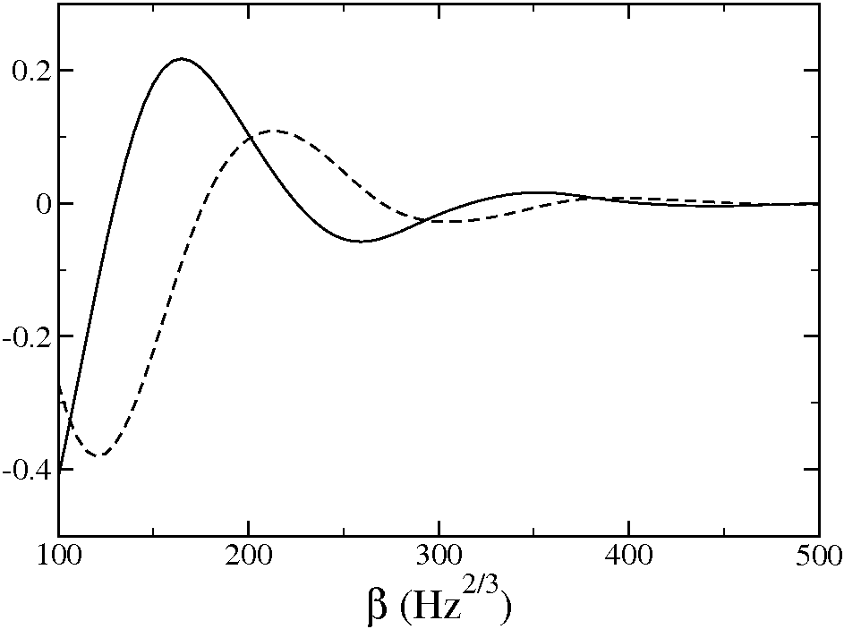
Figure 2.11: Plot of $C_{7}$ (solid line) and $S_{7}$ (dashed-line) that are defined in Eq. (2.5.2). For values of $\beta\gtrsim 200\rm{Hz}^{2/3}$ the value of both functions drop below $0.1$. For these high values of $\beta$, i.e., the regime of strong modulation, we find that the basis templates Eq. (2.5.2) will be orthogonal to each other without need for the Gram-Schmidt procedure. This in turn will simplify the calculation of the metric. This figure was originally produced by Dr. Benjamin Owen.

Therefore, by making the strong modulation approximation we can write

$$\rho^{2}=\sum_{j=1}^{2n}\left<x,\alpha_{j}h_{j}\right>^{2}$$ (2.70)

similarly to how we construct $\rho^{2}$ for our basis templates $\hat{h}_{j}$ which were orthonormalised by the Gram-Schmidt procedure. We can write the detection template with intrinsic parameters $(\psi_{\rm{NM}}+d\psi_{\rm{NM}},\beta+d\beta)$ as

$$h(f) = (\alpha_{1}+i\alpha_{2})e^{i(\psi_{\mathrm{NM}}+d\psi_{\mathrm{NM}})}$$ (2.71)

$$+(\alpha_{3}+i\alpha_{4})\cos([\beta+d\beta]f^{-2/3})e^{i(\psi_{\mathrm{NM}}+d\psi_{\mathrm{NM}})}$$

$$+(\alpha_{5}+i\alpha_{6})\sin([\beta+d\beta]f^{-2/3})e^{i(\psi_{\mathrm{NM}}+d\psi_{\mathrm{NM}})}$$

Expanding the intrinsic parameters up to their second derivatives we find

$$h(f) \approx \left(1+i\,d\psi_{\mathrm{NM}}-\frac{1}{2}d\psi_{\mathrm{NM}}^{2}\right)\Bigg{\{}(\alpha_{1}+i\alpha_{2}){h}_{1}$$ (2.72)

$$+(\alpha_{3}+i\alpha_{4})\left[\left(1-\frac{1}{2}d\mathcal{B}^{2}\right){h}_{2}-d\mathcal{B}{h}_{3}\right]$$

$$+(\alpha_{5}+i\alpha_{6})\left[\left(1-\frac{1}{2}d\mathcal{B}^{2}\right){h}_{3}+d\mathcal{B}{h}_{2}\right]\Bigg{\}}.$$

where we have used $d\mathcal{B}=d\beta f^{-2/3}$. We define the functional $F$ (originally defined in Owen (1996) [111] as $\mathcal{J}$) as

$$F(a)=\frac{1}{I_{7}}\int_{f_{\rm min}/f_{0}}^{f_{\rm max}/f_{0}}dx\frac{x^{-7/3}}{S_{h}(xf_{0})}a(x)$$ (2.73)

and the noise moment $I$ is itself defined as

$$I_{q}\equiv\int_{f_{\rm min}/f_{0}}^{f_{\rm max}/f_{0}}dx\frac{x^{-q/3}}{S_{h}(xf_{0})}$$ (2.74)

where $f_{\rm min}$ and $f_{\rm max}$ define the range of frequencies we integrate over. Since we have shown that our basis templates Eq. (2.5.2) are orthogonal when the waveforms are strongly modulated we are able to write the overlaps between the detection template $h$ and its constituent basis templates $h_{j}$ as

$$\left<h,h_{1}\right> = \alpha_{1}\left[1-\frac{1}{2}F\left(d\psi_{\mathrm{NM}}^{2}\right)\right]-\alpha_{2}F(d\psi_{\mathrm{NM}}),$$ (2.75)

$$\left<h,h_{4}\right> = \alpha_{2}\left[1-\frac{1}{2}F\left(d\psi_{\mathrm{NM}}^{2}\right)\right]+\alpha_{1}F(d\psi_{\mathrm{NM}}),$$

$$\left<h,h_{2}\right> = \alpha_{3}\left[1-\frac{1}{2}F\left(d\psi_{\mathrm{NM}}^{2}\right)-\frac{1}{2}F\left(d\mathcal{B}^{2}\right)\right]$$

$$\,-\alpha_{4}F(d\psi_{\mathrm{NM}})+\alpha_{5}F(d\mathcal{B})-\alpha_{6}F(d\psi_{\mathrm{NM}}\,d\mathcal{B}),$$

$$\left<h,h_{5}\right> = \alpha_{4}\left[1-\frac{1}{2}F\left(d\psi_{\mathrm{NM}}^{2}\right)-\frac{1}{2}F\left(d\mathcal{B}^{2}\right)\right]$$

$$\,+\alpha_{3}F(d\psi_{\mathrm{NM}})+\alpha_{6}F(d\mathcal{B})+\alpha_{5}F(d\psi_{\mathrm{NM}}\,d\mathcal{B}),$$

$$\left<h,h_{3}\right> = \alpha_{5}\left[1-\frac{1}{2}F\left(d\psi_{\mathrm{NM}}^{2}\right)-\frac{1}{2}F\left(d\mathcal{B}^{2}\right)\right]$$

$$\,-\alpha_{6}F(d\psi_{\mathrm{NM}})-\alpha_{3}F(d\mathcal{B})+\alpha_{4}F(d\psi_{\mathrm{NM}}\,d\mathcal{B}),$$

$$\left<h,h_{6}\right> = \alpha_{6}\left[1-\frac{1}{2}F\left(d\psi_{\mathrm{NM}}^{2}\right)-\frac{1}{2}F\left(d\mathcal{B}^{2}\right)\right]$$

$$\,+\alpha_{5}F(d\psi_{\mathrm{NM}})-\alpha_{4}F(d\mathcal{B})-\alpha_{3}F(d\psi_{\mathrm{NM}}\,d\mathcal{B}).$$

Using Eq. (2.70) we can write the square of the overlap when filtering a detection template $h(\psi_{\mathrm{NM}},\beta)$ with another detection template $h(\psi_{\mathrm{NM}}+d\psi_{\mathrm{NM}},\beta+d\beta)$ as

$$\rho^{2} = \sum_{j=1}^{6}\left<h,h_{j}\right>^{2}$$ (2.76)

$$= \sum_{j=1}^{6}\alpha_{j}^{2}\left[1-F(d\psi_{\mathrm{NM}}^{2})+F(d\psi_{\mathrm{NM}})^{2}\right]-\sum_{j=3}^{6}\alpha_{j}^{2}\left[F(d\mathcal{B}^{2})-F(d\mathcal{B})^{2}\right]$$

$$-\bigg{[}2\left(\alpha_{3}\alpha_{6}\right.-\left.\alpha_{4}\alpha_{5}\right)\times\left[F(d\psi_{\mathrm{NM}}\,d\mathcal{B})-F(d\psi_{\mathrm{NM}})F(d\mathcal{B})\right]\bigg{]}.$$

We maximise $\rho^{2}$ subject to the constraint $\sum_{j=1}^{2n}\alpha_{j}^{2}=1$ using the method of Lagrange multipliers (see Eq. (2.49)). We find $\alpha_{1}=\alpha_{2}=0$, $\alpha_{3}=-\alpha_{6}$, and $\alpha_{4}=\alpha_{5}$, which leads to

$$\rho^{2} = 1-F(d\psi_{\mathrm{NM}}^{2})+F(d\psi_{\mathrm{NM}})^{2}-F(d\mathcal{B}^{2})$$ (2.77)

$$+F(d\mathcal{B})^{2}+F(d\psi_{\mathrm{NM}}\,d\mathcal{B})-F(d\psi_{\mathrm{NM}})F(d\mathcal{B}).$$

As well as maximising $\rho^{2}$ with respect to the $\alpha_{j}$ parameters we should also maximise with respect to the time of the sources coalescence $t_{c}$. During matched-filtering we maximise over time using an FFT (see Sec. 2.4.1). Here we will consider a signal perfectly described by a template $h(\psi_{\rm{NM}}+d\psi_{\rm{NM}},\beta+d\beta,t_{c}+dt_{c})$. We can incorporate the time dependence of the template into our phase by writing $\psi=\psi_{\rm{NM}}+2\pi ft_{c}$. To calculate the dependence on time of the match between two signals $h(\psi_{\rm{NM}},\beta,t_{c})$ and $h(\psi_{\rm{NM}}+d\psi_{\rm{NM}},\beta+d\beta,t_{c}+dt_{c})$ we will replace $d\psi_{\rm{NM}}$ with $d\psi=\psi_{0}f^{-5/3}+d\psi_{3}f^{-2/3}+2\pi fdt_{c}$ in Eq. (2.77).

Using Eq. (2.63) for the mismatch we can write

$$\rho^{2}=1-2g_{ab}d\lambda^{a}d\lambda^{b}$$ (2.78)

(where we have used match $M=\rho$ for the case of normalized templates without noise) allowing us to identify the metric’s components (which we will now call $\gamma_{ab}$) as

$$\gamma_{t_{c}t_{c}} = 2\pi^{2}\left(J_{1}-J_{4}^{\phantom{4}2}\right),$$

$$\gamma_{t_{c}\psi_{0}} = \pi\left(J_{9}-J_{4}J_{12}\right),$$

$$\gamma_{t_{c}\psi_{3}} = \pi\left(J_{6}-J_{4}J_{9}\right),$$

$$\gamma_{t_{c}\beta} = \frac{\pi}{2}\left(J_{6}-J_{4}J_{9}\right),$$

$$\gamma_{\psi_{0}\psi_{0}} = \frac{1}{2}\left(J_{17}-J_{12}^{\phantom{12}2}\right),$$

$$\gamma_{\psi_{0}\psi_{3}} = \frac{1}{2}\left(J_{14}-J_{9}J_{12}\right),$$

$$\gamma_{\psi_{0}\beta} = \frac{1}{4}\left(J_{14}-J_{9}J_{12}\right),$$

$$\gamma_{\psi_{3}\psi_{3}} = \frac{1}{2}\left(J_{11}-J_{9}^{\phantom{9}2}\right),$$

$$\gamma_{\psi_{3}\beta} = \frac{1}{4}\left(J_{11}-J_{9}^{\phantom{9}2}\right),$$

$$\gamma_{\beta\beta} = \frac{1}{2}\left(J_{11}-J_{9}^{\phantom{9}2}\right)$$ (2.79)

where $J$ represent the normalized noise moments given by Poisson and Will (1995) [118]

$$J_{q}\equiv\frac{I_{q}}{I_{7}}$$ (2.80)

and the noise moment $I$ was defined in Eq. (2.74).

We are interested in placing templates in the ($\psi_{0}$, $\psi_{3}$, $\beta$) space so we will project out the time dependence of the metric using (from Owen (1996) [111] Eq. (2.28)):

$$g_{ij}=\gamma_{ij}-\frac{\gamma_{ti}\gamma_{tj}}{\gamma_{tt}}$$ (2.81)

where the indices $i$ and $j$ range over all the intrinsic parameters ($\psi_{0}$, $\psi_{3}$, $\beta$). As well as projecting out the time dependence we also neglect the $\psi_{0}\beta$ and $\psi_{3}\beta$ cross terms which will simplify the template placement and only result in a small over-coverage of the parameter space (neglecting these terms will only decrease the volume of parameter space a given template achieves match greater than minimal match by $\sim 3\%$). The metric we finally obtain has components

$$g_{\psi_{0}\psi_{0}} = \frac{1}{2}\left(J_{17}-J_{12}^{\phantom{12}2}\right)-\frac{\left(J_{9}-J_{4}J_{12}\right)^{2}}{2\left(J_{1}-J_{4}^{\phantom{4}2}\right)},$$

$$g_{\psi_{0}\psi_{3}} = \frac{1}{2}\left(J_{14}-J_{9}J_{12}\right)-\frac{(J_{9}-J_{4}J_{12})(J_{6}-J_{4}J_{9})}{2\left(J_{1}-J_{4}^{\phantom{4}2}\right)},$$

$$g_{\psi_{0}\beta} = 0,$$

$$g_{\psi_{3}\psi_{3}} = \frac{1}{2}\left(J_{11}-J_{9}^{\phantom{9}2}\right)-\frac{(J_{6}-J_{4}J_{9})^{2}}{2\left(J_{1}-J_{4}^{\phantom{4}2}\right)},$$

$$g_{\psi_{3}\beta} = 0,$$

$$g_{\beta\beta} = \frac{1}{2}\left(J_{11}-J_{9}^{\phantom{9}2}\right)-\frac{(J_{6}-J_{4}J_{9})^{2}}{8\left(J_{1}-J_{4}^{\phantom{4}2}\right)}.$$ (2.82)

Choosing the upper frequency cutoff

In practice, our upper bound on frequency is the Nyquist frequency $f_{\rm{Nyquist}}=2048\rm{Hz}$ which is defined as half of the sampling frequency $f_{s}=4096\rm{Hz}$ . Ideally, we would perform the integrals to find the moment functions (see Eqs.(2.73) and (2.74)) required in our calculation of the template placement metric up to the upper frequency cutoff $f_{\rm{cut}}$ of our detection templates. For simplicity we use $f_{\rm{Nyquist}}$ as the upper frequency cutoff in these integrals. We find later that despite this approximation our template bank achieves high matches for a range of simulated signals (see Sec.2.5.4).

However, we still must provide an estimate of $f_{\rm{cut}}$ in order to limit our detection templates to the frequencies in which we believe they adequately describe true gravitational waveforms that would be observed (i.e., the adiabatic limit). We know that after the last stable orbit (LSO, similar to the minimum energy circular orbit which is the termination point of the target waveform) the binary’s components will “plunge” and the bodies will merge over a time scale of only very few inspiral orbits. Clearly, the binary is no longer in the adiabatic regime during its plunge and we choose to set $f_{\rm{cut}}$ to the frequency of the last stable orbit $f_{\rm{LSO}}$.

Determining $f_{\rm{LSO}}$ is complicated except in the extreme asymmetric mass ratio limit ($\eta\rightarrow 0$). We approximate the gravitational wave frequency of the last stable orbit (LSO) as the highest gravitational wave frequency that would be emitted by test mass in Schwarzschild geometry:

$$f_{\rm{LSO}}=\frac{1}{6^{3/2}\pi M}.$$ (2.83)

In practice we estimate $M$ to be the total mass of our binary from the non-physical parameters of our template bank $\psi_{0}$ and $\psi_{3}$ using Eqs. (2.56) and (2.57). For reference, a binary with total mass $M=1M_{\odot}$ would have $f_{\rm{LSO}}\simeq 4400\rm{Hz}$ and a binary with total mass $M=40M_{\odot}$ would have $f_{\rm{LSO}}\simeq 110\rm{Hz}$. The $f_{\rm{LSO}}$ calculated is very much an upper limit on the extent of the inspiral stage of the binary’s evolution and it is likely that the evolution will have become non-adiabatic (Allen et al. (2005) [7]). Despite these limitations, using $f_{\rm{cut}}$ rather than $f_{\rm{Nyquist}}$ will improve the matches obtained by our templates with expected inspiral signals.

We know from the studies presented in BCV2 [40] (see Figs. 5 and 6 and surrounding text) that the optimal value of $f_{\rm{cut}}$ depends on $\kappa$ (related to the opening angle of the spin and orbital angular momenta, see Eq. (2.31)). Future searches could benefit from allowing multiple values of $f_{\rm{cut}}$ to be specified for each $(\psi_{0},\psi_{3},\beta)$ combination present in the template bank. The choice of the lower frequency is dependent on the noise spectrum of the detectors and is discussed in Sec. 2.6.3.

2.5.3 Template placement algorithm

The spacing of our templates (i.e., the density of our template bank) is determined by our choice of the minimal match ($MM$) which is defined as the lowest match that can be obtained between a signal and the nearest template, see Owen (1996) [111] and Sathyaprakash and Dhurandhar (1991) [127]. A template bank with minimal match $MM=0.95$ would, therefore, suffer no more than a $1-MM=5\%$ loss in SNR due to mismatch between the parameters of a signal and the best possible template in the bank (assuming that the signal and templates are from the same family, i.e., a fitting factor of unity).

The metric components shown in Eq. (2.5.2) are not dependent on the intrinsic parameters ($\psi_{0}$, $\psi_{3}$, $\beta$) which makes the placement of templates simple. The templates are placed on the vertices of a body-centred cubic (BCC) lattice which is the most efficient template placement in three dimensions (i.e., it leads to the smallest number of templates to cover a given region of parameter space).

The metric $g$ (whose components are given in Eq. (2.5.2)) is diagonalized to form $\mbox{\boldmath$g$}^{\prime}$ which will only have components $g_{\psi_{0}\psi_{0}}^{\prime}$, $g_{\psi_{3}\psi_{3}}^{\prime}$ and $g_{\beta\beta}$ (the $\beta\beta$ component is unaffected by the diagonalization).

The spacings of the template banks (in a single direction and ignoring the others) which yield matches of at least the minimal match $MM$ is given by $ds_{i}^{\phantom{i}2}=2(1-MM)=g_{ii}\Delta(\lambda^{i})^{2}$. The factor of 2 is so that the point where the match is at its worst (i.e., $MM$) is equidistant between two templates in the $\lambda^{i}$ direction. This can be rearranged to find the co-ordinate spacing $\Delta\mbox{\boldmath$\lambda$}$ of our intrinsic parameters for a given minimal match. For body centred cubic placement we require

$$\Delta\psi_{0}^{\prime} = \frac{4}{3}\sqrt{\frac{2(1-MM)}{g_{\psi_{0}\psi_{0}}^{\prime}}},$$ (2.84)

$$\Delta\psi_{3}^{\prime} = \frac{4}{3}\sqrt{\frac{2(1-MM)}{g_{\psi_{3}\psi_{3}}^{\prime}}},$$ (2.85)

$$\Delta\beta = \frac{2}{3}\sqrt{\frac{2(1-MM)}{g_{\beta\beta}}}.$$ (2.86)

We will place templates in order to capture systems with asymmetric masses for which the spin angular momenta is generally larger than the orbital angular momentum leading to more pronounced spin effects. We estimate the range of $\psi_{0}$ and $\psi_{3}$ values needed to cover the physical mass range $1.0M_{\odot}<m_{1}<3.0M_{\odot}$ and $6.0M_{\odot}<m_{2}<12.0M_{\odot}$ using the relationships given by Eqs. (2.56) and (2.57). This choice of mass region allows us to concentrate on asymmetric mass ratio binaries with total mass low enough that we can use $f_{\rm{Nyquist}}$ as the upper frequency when evaluating moments for the template bank metric calculation. Due to the approximate nature of these relationships we find that the range of masses the template bank achieves best matches for is slightly different and this is discussed in Sec. 2.5.4. These choices lead to placing templates with $\psi_{0}$ in the range $\sim 2-8\times 10^{5}\rm{Hz}^{5/3}$ and $\psi_{3}$ in the range $\sim-2--5\times 10^{3}\rm{Hz}^{2/3}$. We place templates with $\beta$ in the range $0-\beta_{\rm{max}}$ where

$$\beta_{\rm{max}}=3.8\pi\left(1+\frac{3}{4}\frac{m_{2,{\rm{max}}}}{m_{1,{\rm{min}}}}\right)\frac{m_{1,{\rm{max}}}}{m_{2,{\rm{min}}}}\left(\frac{10M_{\odot}}{m_{1,\rm{min}}+m_{2,\rm{min}}}\frac{10\rm{Hz}}{150\rm{Hz}}\right)^{2/3}$$ (2.87)

is chosen to give the highest value of $\beta$ possible given the mass range we are seeking to cover and the peak sensitivity of the detector occurring at roughly $f=150\rm{Hz}$. By placing templates with small values of $\beta$ we will be sensitive to weakly spin-modulated binaries as well as the strongly modulated binaries the template bank was designed to cover.

Starting at the lowest values of $\psi_{0}^{\prime}$, $\psi_{3}^{\prime}$ and $\beta$ we place templates in a grid in the plane of constant $\beta=0$ using the co-ordinate spacings for $\psi_{0}^{\prime}$ (Eq. (2.84)) and $\psi_{3}^{\prime}$ (Eq. (2.85)). We then move to the next layer of $\beta$ using Eq. (2.86) and then place another grid of templates. Neighbouring layers of templates will have their $\psi_{0}^{\prime},\psi_{3}^{\prime}$ co-ordinate values offset from each other by $\Delta\psi_{0}^{\prime}/2,\Delta\psi_{3}^{\prime}/2$ in order to create the body-centred cubic spacing.

We only place templates within the range of $\psi_{0},\psi_{3},\beta$ described above. This can lead to the template bank having ragged edges and some under-coverage of the targeted region of parameter space near the boundary of the template bank. Owen and Hanna developed a scheme to solve this problem: if the next template to be placed using co-ordinate spacing $\Delta x$ (where $x$ is $\psi_{0}^{\prime}$, $\psi_{3}^{\prime}$ or $\beta$) according to Eqs.(2.84) to (2.86) would be beyond the boundary of the template bank they assess whether a template placed using spacing $\Delta x/2$ would be within the boundary of the template bank. If so, this template is included in the template bank. Figure 2.12 shows an example of a template bank generated during the search of S3 LIGO data.

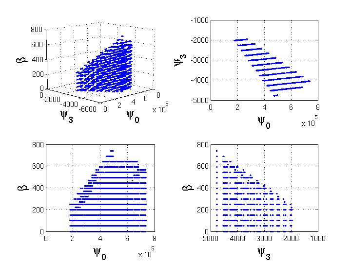
Figure 2.12: A template bank generated with minimal match $=0.95$ using 2048 seconds of H1 data taken during S3. The crosses show the positions of individual templates in the $(\psi_{0},\psi_{3},\beta)$ parameter space. For each template a value for the cutoff frequency $f_{\rm cut}$ is estimated using Eq. (2.83). This bank requires a 3-dimensional template placement scheme in order to place templates in the $(\psi_{0},\psi_{3},\beta)$ parameter space. Previous searches for non-spinning systems have used 2-dimensional placement schemes.

2.5.4 Testing the template bank

The template bank was tested using a series of simulated signals constructed using the equations of the target waveforms described in Sec. 2.2. We considered a variety of spin configurations including systems where neither, one or both bodies were spinning. We also considered masses outside the range we expected the template bank to have good coverage in order to fully evaluate the range of masses for which it could be used. For each spin configuration we created a series of signals for every combination of (integer) masses in the range: $1.0~{}M_{\odot}<m_{1},m_{2}<20.0~{}M_{\odot}$. Using the initial LIGO design sensitivity we then measured the best match that could be obtained for each signal using our template bank. Figure 2.13 shows a sample of the results from the tests of the template bank. As expected we found that our template bank achieved the highest matches for non-spinning (and therefore non-precessing) binaries. Performance degrades as spin-precessional effects become more pronounced i.e., when both bodies are spinning maximally with spins misaligned from the orbital angular momenta. The template achieved matches $>0.9$ for a mass range $1.0~{}M_{\odot}<m_{1}<3.0~{}M_{\odot}$ and $12.0~{}M_{\odot}<m_{2}<20.0~{}M_{\odot}$ (and equivalent systems with $m_{1}$ and $m_{2}$ swapped). The detection template family (described in Sec. 2.4) is capable of obtaining high matches for comparable mass systems, the lower matches obtained for comparable mass systems are a result of targeting our template bank on asymmetric mass ratio systems (which are more susceptible to spin effects and conform to the strong modulation approximation).

Matches below the specified minimal match of $0.95$ in the bank’s region of good coverage are a consequence of (small) differences between the DTF and the target waveforms meaning that the DTF cannot perfectly match the target waveforms (see discussion of the fitting factor of the DTF in Sec. 2.4).

The fitting factor (see Sec. 2.3) measures the reduction of SNR due to differences between the DTF and the target waveform [10] and should not be confused with the minimal match which measures the loss of SNR due to discreteness of the template bank [111]. The DTF performance was evaluated and its fitting factor was measured in Sec. VI of Ref. [40], for NS-BH systems an average FF of $\approx 0.93$ was measured.

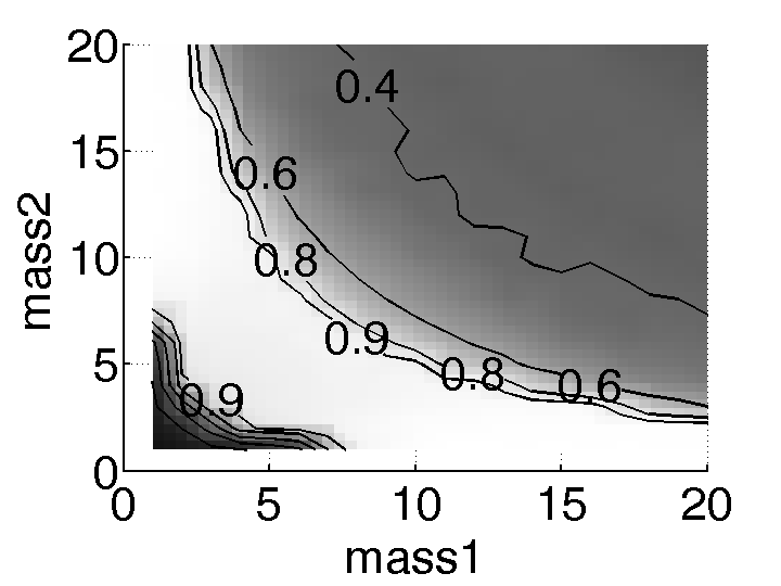
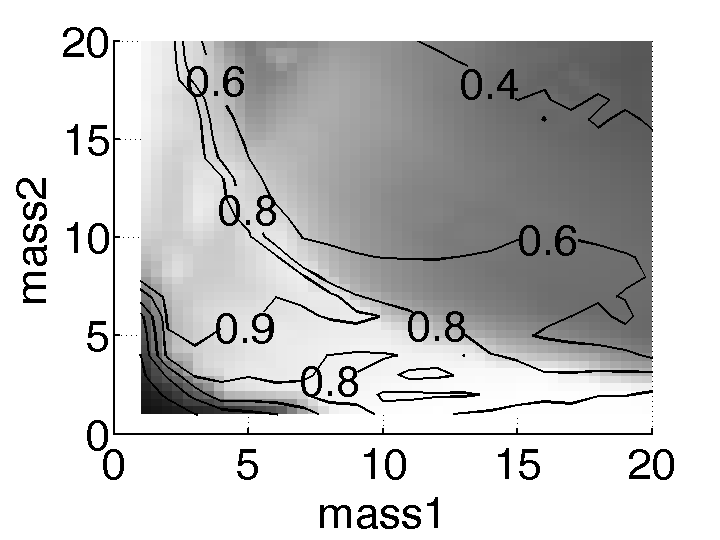
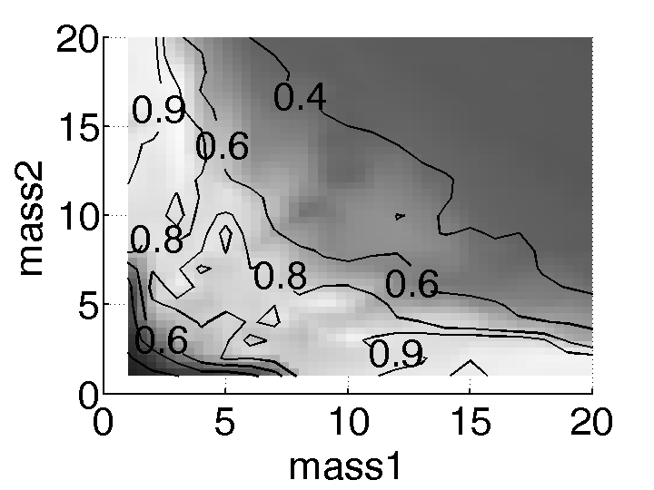
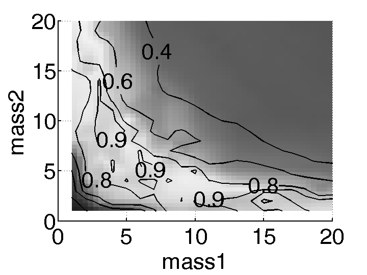
Figure 2.13: Plots showing the best match achieved by filtering a series of simulated signals through the template bank described in this Section. The values on the $x$ and $y$ axes correspond to the component masses of the binary source to which the simulated signal corresponds. The colour of the plots shows the best match achieved for a given simulated signal. The four subplots correspond to four different spin-configurations of the binary source. The top-left subplot shows results for a non-spinning binary system. The top-right subplot shows results for a system consisting of one non-spinning object and one maximally spinning object with its spin slightly misaligned with the orbital angular momentum. We would expect this system to precess. The bottom two subplots show results for two generic precessing systems consisting of two maximally spinning bodies with spins and orbital angular momentum all misaligned from each other. We see that the region of the mass plane for which we obtain matches $>0.9$ is largest for the non-spinning system and tends to be concentrated in the asymmetric mass region loosely bounded by $1.0~{}M_{\odot}<m_{1}<3.0~{}M_{\odot}$ and $12.0~{}M_{\odot}<m_{2}<20.0~{}M_{\odot}$.

2.6 The data analysis pipeline

The analysis of real detector data can be divided into a series of well defined processes that are collectively known as the data analysis pipeline. Figure 2.14 shows the data analysis pipeline that was used in the analysis of LIGO data taken during its third science run (S3, see Sec. 2.6.3). The pipeline used for this search is the same as was used in searches for non-spinning binaries in S3 LIGO data. The searches for primordial black holes, binary neutron star and binary black holes with non-spinning components using S3 and S4 LIGO data are described in Ref. [5].

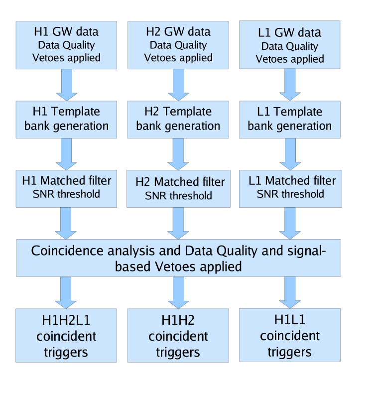
Figure 2.14: Flowchart showing the various stages of the data analysis pipeline. For each of the LIGO detectors, H1, H2 and L1 (see Sec. 1.3.3 for a description) we begin our analysis by discarding data taken during times when there are known environmental disturbances or problems with the detector (Secs. 2.6.1 to 2.6.3). We generate a template bank for each detector (Sec. 2.6.4) and then subsequently matched-filter the data (Sec. 2.6.5) constructing a list of triggers with signal to noise ratio exceeding our predetermined threshold. Triggers occurring within a small time window, with similar parameters consistent with those expected to be caused by true gravitational wave signals in two or more detectors are identified (Secs. 2.6.6 to 2.6.8) as coincident triggers. Coincident triggers are then investigated to see if they are consistent with our predicted background and whether they could be confidently claimed as evidence for a gravitational wave (Sec. 2.7).

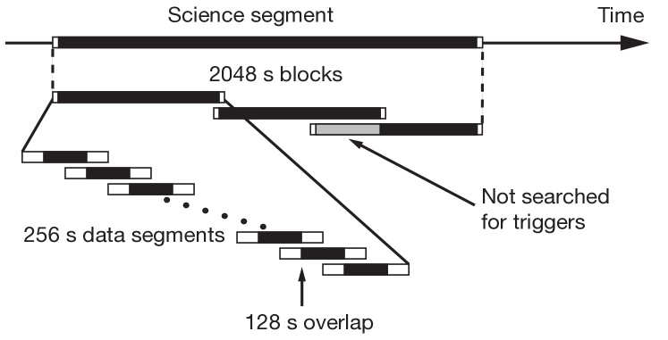
Figure 2.15: Figure showing the subdivision of a science segment. This figure, originally produced by Duncan Brown, was reproduced from B. Abbot et al., Phys. Rev. D 72, 082001 (2005) [3], with permission from the authors.

2.6.1 Data selection

The matched-filter is found to be the optimal filter to find a known signal in stationary and Gaussian noise. In reality, we find that our detector data is neither Gaussian or stationary.

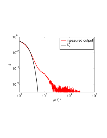
Figure 2.16: Histograms of $\rho^{2}$ measured when matched-filtering real LIGO L1 data taken during S3 with BCV2 templates with i) $\beta=0$ (left hand plot) and ii) $\beta\neq 0$ (right hand plot). In Fig. 2.8 we confirmed that $\rho^{2}$ will be distributed as a $\chi_{n}^{2}$ when the filtered data is Gaussian. On the plots above we see an excess in the distribution of our measured output at high values of $\rho^{2}$ indicating that our real detector data is non-Gaussian. These high SNR events are caused by transients in the detector data and in Sec. 2.6.1 we describe how data taken during times when the detector was performing poorly or when there was a known disturbance is excluded from our analysis.

For Gaussian data we would expect the square of the SNR, $\rho^{2}$ obtained using the matched-filter templates of our DTF to follow a $\chi^{2}$ distribution with 2 degrees of freedom when $\beta=0$ and 6 degrees of freedom when $\beta\neq 0$ (see Sec. 2.4.2). Figure 2.16 shows a comparison between the distribution of $\rho^{2}$ we measured using real LIGO L1 data and the $\chi^{2}$ distribution we would expect to observe if the data was truly Gaussian. We observe a tail of high SNR triggers when matched-filtering the real data indicating that the data is non-Gaussian. Figure 2.18 shows the amplitude spectra for H2 estimated at two different times during S3. We observe a flattening of the spectra as S3 progresses showing that the data is not stationary. Also, in Gonzalez (2003) [74] (also see [122]) the authors introduce the Rayleigh monitor which assesses how Gaussian and stationary an interval of data is. A variant of this monitor is being used in more recent analysis of LIGO data.

Indeed, transients in the data due to problems with the detector or environmental disturbances can lead to a huge number of false alarm triggers, i.e., triggers caused by something other than a true gravitational wave signal. Stretches of data during which the detector had poor performance or when there was an environmental disturbance will be excluded from analysis. The study of the detector’s behaviour is called detector characterisation. The detector characterisation carried out on S3 LIGO data is detailed in Christensen (for the LIGO Scientific Collaboration, 2005) [45].

We categorise times when we know the detector had poor operation with data quality (DQ) flags. Below we list and briefly describe the DQ flags used in this search (which were also used in all searches for inspiral signals in S3 data). The numbers in brackets following the name of the DQ flag indicate the percentage of data associated with that flag.

• NO_DATA ($0.01\%$): Some fault meant that the detector was not collecting data during these times.

• NO_RDS ($0.02\%$): Under normal operation, we create a number of reduced data sets (RDS) which contain a down-sampled time series of the gravitational wave channel as well as a selection of the auxiliary channels. This flag indicates that there was some error meaning that the reduced data set was not created.

• UNLOCKED ($0.03\%$):  When the detector is working correctly, the test mass mirrors of the interferometer will be “locked” into place so that the laser beam will resonate in the optical cavity in each arm (see Sec. 1.3.3). This flag indicates that the detector has become unlocked.

• INVALID_TIMING ($2.3\%$): This flag indicates that the time-stamping of the data taken by the detector is not valid. Knowledge of the exact time that data was taken is crucial if we are to associate an event measured in one detector with an event occurring in another detector (see Sec. 2.6.6). Also, the accuracy of timing directly affects the accuracy to which we can determine the sky location of a gravitational source by triangulation.

• CALIB_LINE_V03 ($2.0\%$): Monochromatic sinusoidal oscillations are applied to the interferometer’s test mass mirrors with known frequency and amplitude. These oscillations appear as spikes, known as calibration lines, in the amplitude spectrum of the gravitational wave channel data. By measuring the amplitude and frequency at which these lines appear in the data it is possible to calibrate the amplitude of the gravitational wave channel strain data [66]. This flag indicates that there is some problem with the oscillation of the test mass mirrors or the measurement of the calibration lines.

• OUTSIDE_S3 ($0.4\%$): The database recording the state of the detector may include details of data taken beyond the end of the S3 run. We will exclude data taken outside of the S3 run.

We construct a list of times for which each detector is operating well in what is known as science mode excluding times associated with various DQ flags. As well as the use of DQ flags, later in the pipeline various short stretches of data will be discarded or vetoed. There are two types of vetoes: signal-based vetoes and detector-based vetoes and these will be discussed in Sec. 2.6.8.

Contiguous stretches of data taken when a detector is in science mode are called science segments. The science segments are divided up into 2048 second blocks. Each block is divided into 15 overlapping 256 second data segments. Figure 2.15 shows a single science segment and how it is divided up for analysis. Each data segment has 64 seconds overlap with the preceding and subsequent data segment (except for the first and fifteenth data segment which only have one adjacent data segment). The power spectrum of each 256 second data segment is estimated using Welch’s method with a Hann window (see Allen et al. (2005) [7] for further details). We then estimate the power spectrum of each 2048 second block as the median average of the power spectra of its 15 data segments. To be clear, we will measure the power contained within a particular frequency bin $f_{i}+\Delta f$ for each of the 15 data segments. We then take the median average of these powers and use that as the power for that frequency bin in the block’s power spectrum. The median average is used rather than the mean to avoid biasing of the average power spectrum by short-duration non-stationary noise events in the data.

There are two reasons we need to overlap data segments (and similarly why we need to overlap 2048 second blocks). This is discussed in detail in Allen et al. (2005) [7] and is briefly summarised here. Firstly, the Fast Fourier Transform (FFT) we use in matched-filtering (see Sec. 5.3) treats each data segment as if it is periodic. The subsequent wrap-around effect causes a stretch of data the length of the template $T_{\rm{Template}}$ to be invalid at the start of each data segment. Secondly, narrow lines (“spikes”) in the inverse noise power spectrum ($S_{n}(f)^{-1}$) used in the inner product (see e.g., Eq. (1.101)) will cause corruption of data throughout each data segment. The inverse noise power spectrum is truncated in the time domain in order to limit the corruption to stretches of data length $T_{\rm{Spec}}$ at the start and end of each data segment. Note that we cannot choose $T_{\rm{Spec}}$ to be arbitrarily small since we would then lose important information about the (inverse) noise power spectrum in the frequency domain. These two effects (wrap-around and “spikes”) lead to stretches of corrupted data of duration $T_{\rm{Template}}+T_{\rm{Spec}}$ at the beginning and $T_{\rm{Spec}}$ at the end of each data segment. In order to avoid corrupted data we only analyse and record triggers from the central 128 seconds of each 256 second data segment and ignore the first and last 64 seconds of each data segment. We then overlap each data segment with the preceding and subsequent data segment by 128 seconds to ensure that all the data will be analysed. We do not analyse the first or last 64 seconds of each 2048 second block and we therefore overlap each block with the preceding and subsequent block by 128 seconds (except for the first and last block in the science segment which only have only have one adjacent block).

At the end of a science segment it might be necessary to overlap the final two 2048 second blocks by more than 128 seconds to ensure that we analyse as much of the remaining data as possible. Care is taken to ensure that the same stretch of data is not analysed twice (i.e., the region marked “Not searched for triggers” in Fig. 2.15). Since it is not possible to overlap a 2048 second blocks at the very beginning or end of a science segment, the first and last 64 seconds of each science segment will not be analysed. Science segments shorter than 2048 seconds in duration will also not be analysed.

2.6.2 Playground data

We specify a subset of our data to be playground data which we use to tune various parameters (e.g., SNR thresholds, coincidence windows). The use of playground data allows the data analyst to tune parameters while remaining blind to the remainder of the data set thus avoiding statistical bias. The set of playground times is defined formally as

$$\mathcal{T}=\left\{t\in\left[t_{n},t_{n}+600\right):t_{n}=729273613+6370n,n\in\mathbb{Z}\right\}$$ (2.88)

where $729273613$ is the GPS time of the beginning of LIGO’s second science run (from internal LIGO technical documents T030256 and T030020). According to this definition playground times will account for, on average, $9.4\%$ of any given stretch of time. Once parameters have been tuned using the playground data, the full data set (including playground) will be searched for gravitational wave events. To avoid statistical bias, the values of the parameters chosen after the analysis of playground data will remain fixed throughout the subsequent analysis of the full data set.

Although it is possible to make a detection of a gravitational wave during playground times, playground times are excluded from any upper limit calculations which are performed when no gravitational waves have been detected.

2.6.3 The S3 data set

The third LIGO science run (S3) took place between October 31st 2003 ($16:00:00$ UTC, $751651213$ GPS) and January 9th 2004 ($16:00:00$ UTC, $757699213$ GPS). Data collected by the LIGO Hanford Observatory (LHO) detectors (i.e., H1 and H2) was only analysed when both detectors were in science mode. This was due to concerns that since both of these detectors share the same vacuum system, the laser beam of a detector in anything but science mode might interfere with the other detector (see Sec. 1.3.1 for a description of the LIGO detectors).

We denote periods of time when all three detectors are in science mode as H1-H2-L1 times and periods when only the LHO detectors are on as H1-H2 times. A coincident trigger consisting of a trigger in the H1 detector and the L1 detector will be referred to as an H1-L1 coincident trigger and similarly for other combinations of detectors. In this search we analysed 184 hours of H1-H2-L1 data and 604 hours of H1-H2 data (see Table 2.2).

Lower frequency cutoff

We must also choose the lower frequency cutoff $f_{\rm{low}}$ which will be the lower limit of any integrals we perform in the frequency domain, e.g., the computation of moments to calculate the template placement metric or the inner product used to calculate the SNR. Note that the upper frequency cutoff will depend on the particular template used and the total mass of the source it represents (see Sec. 2.5.2).

There are competing factors that influence the choice of $f_{\rm{low}}$. Binaries with larger masses will plunge and coalesce at lower frequencies (see Eq. (2.83)). Taking lower values of $f_{\rm{low}}$ means that we will be sensitive to binaries with larger total mass and will also observe more orbital cycles of inspiraling binaries in general. The observation of more cycles allows for greater SNR’s to be achieved but would require longer duration templates (and simulated waveforms) to be produced which would increase the computational cost of the search. This increase in computational cost is far less for searches employing templates which are generated in the frequency (rather than time) domain, such as the BCV2 DTF used in this analysis. Note also, that although increasing the mass range of a search to include heavier binaries will increase the number of templates in the bank (for a given minimal match), the number of templates required to cover the higher-mass region of parameter space is far smaller than the number of templates required to cover the low-mass region (see, for example Fig. 5 of Babak et al. (2006) [17]). However, at lower frequencies seismic activity causes the sensitivity of ground-based detectors to become worse and the spectrum to be non-stationary (see Sec. 1.3.1).

In practice we take the lowest value of $f_{\rm{low}}$ for which the noise spectrum is approximately stationary. For searches of S3 LIGO data a value of $f_{\rm{low}}=70\rm{Hz}$ was chosen. As the detectors achieve better sensitivity and greater stationarity of noise, the values of $f_{\rm{low}}$ we use have decreased allowing higher mass binaries to be searched for. In searches of S4 and S5 LIGO data, lower cutoff frequencies as low as $f_{\rm{low}}=40\rm{Hz}$ have been used.

Table 2.2: Summary of the amount of data analysed in our various data sets. In S3 we only analyse data from the LHO detectors when both H1 and H2 are in science mode. Around $9.4\%$ of the data is classified as playground data and is used to tune the parameters of the search. Playground data is not included in the upper limit calculation but is still searched for possible detections.

Data type	Total analysed (hours)	Non-playground (hours)
H1-H2	604	548
H1-H2-L1	184	167

2.6.4 Template bank generation

Using the estimated PSD we will calculate the template placement metric Eq. (2.62) and create a template bank for each 2048s blocks of data for each detector (H1, H2 and L1). The metric calculation and template placement scheme used in this search is described in Sec. 2.5.

In this search we use a minimal match of $0.95$. Figure 2.17 shows the number of templates in each template bank against GPS time throughout S3. We see a large increase in the size of the H2 template banks which was caused by a flattening of the its power spectral density profile as S3 progressed (see Fig. 2.18). The output of template bank generation will be a list of the $\psi_{0}$, $\psi_{3}$ and $\beta$ values that we are required to search over for each 2048 second block for each detector.

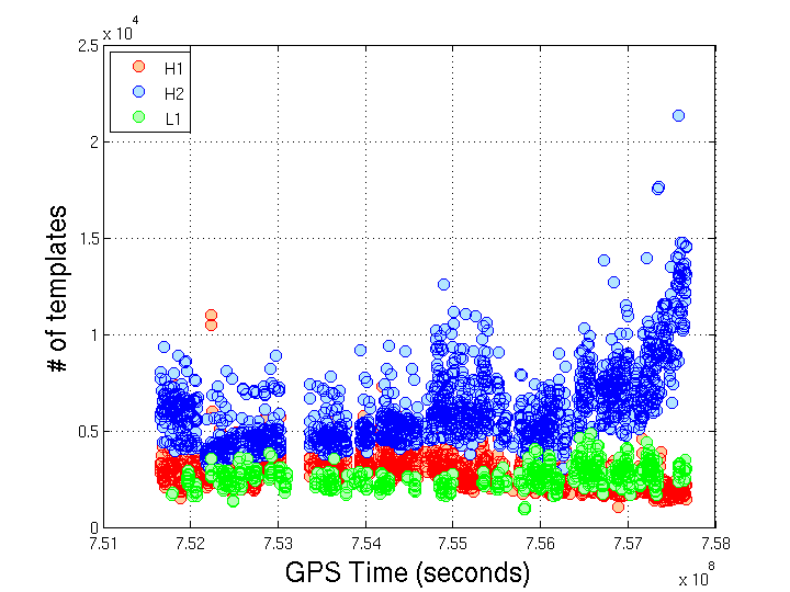
Figure 2.17: Number of templates in each template bank. We generate a separate template bank for each 2048s block of data for each detector. We then matched-filter each template in the bank against the block of data and generate a list of triggers which have SNR exceeding our threshold. See Secs. 2.6.4 and 2.6.5 for further details. The large increase (a factor of $\sim 6$) in the size of the H2 template banks was caused by a flattening of the its amplitude (and therefore power) spectral density profile as S3 progressed. Figure 2.18 compares the amplitude spectra of H2 at two different times during S3.

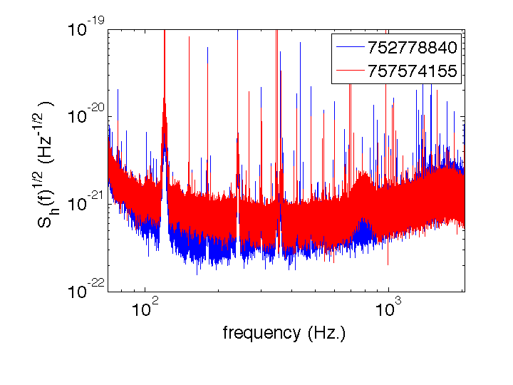
Figure 2.18: Amplitude spectral density curves for H2 estimated at two different times during S3. The GPS times in the legend of this plot indicate the start time of the 2048s block of data that was used to estimate the spectrum. As S3 progresses the amplitude (and therefore power) spectra of H2 become flatter which leads to the increase in the number of templates required for H2 as shown in Fig. 2.17.

2.6.5 Matched-filtering of detector data

We matched-filter every 2048s block of data using each template in the associated template bank. If the SNR measured by a particular template exceeds the SNR threshold, we record a trigger which contains details of the template and the time at which the SNR threshold was exceeded. In practice we take the FFT of each 256 second data segment and matched-filter each separately. We do this because the power spectrum we use in the matched-filter has the frequency resolution of the FFT of a 256 second data segment due to the way we estimate it (see Sec. 2.6.1).

For Gaussian white noise, $\rho^{2}$ will, in general, have a $\chi^{2}$ distribution with 6 degrees of freedom. In the case where the spin parameter $\beta=0$ we find that $\mathcal{\widehat{A}}_{2}$ and $\mathcal{\widehat{A}}_{3}$ both vanish and that $\rho^{2}$ is described by a $\chi^{2}$ distribution with 2 degrees of freedom. To reflect the increased freedom we choose a higher SNR threshold, $\rho_{*}=12$ when $\beta\neq 0$ and a lower value of $\rho_{*}\approx 11.2$ when $\beta=0$. These values were chosen to give approximately the same number of triggers when analysing Gaussian white noise and to ensure that the number of triggers produced during the real search was manageable.

We perform two stages of clustering in order to reduce the number of triggers we are required to store. The first stage involves identifying all triggers with SNR greater than our thresholds that were generated from one particular template. We record only the trigger with the highest SNR over a stretch of data and discard any other triggers generated by the same template within 16 seconds of it. The second stage involves recording only the trigger with the highest SNR in each $100$ms stretch of data regardless of which template was used to generate it.

Due to the huge number of templates required by H2 during the end of S3 we expected that the number of triggers generated might cause the search to become computationally unfeasible. However, through use of the clustering methods described here the number of triggers recorded by the matched-filtering of H2 data was reduced to such a level ($\sim 5\times 10^{4}$ triggers per 2048 second block) that we decided to analyse data from all three LIGO detectors. The output of the matched-filter stage is the list of triggers with SNR exceeding the SNR threshold that survive clustering for each detector. Each trigger will contain information including the time $t$ it was recorded, the values of the intrinsic parameters of the template that was used to generate it (i.e., $\psi_{0},\psi_{3},\beta,f_{\rm{cut}}$), its SNR $\rho$ and the values of the other extrinsic parameters $\alpha_{1\dots 6}$ that were used to obtain the (maximised) SNR.

We know that the amplitude of the gravitational wave emitted by an inspiraling binary increases throughout the inspiral stage of its evolution before its components plunge and coalesce. We expect that the time at which we measure the maximum SNR for a true gravitational signal from a binary will correspond to the end of the inspiral stage of its evolution and, therefore, approximately to the (retarded) time of its coalescence. The time recorded in our trigger is called the coalescence time.

2.6.6 Coincidence analysis

To minimize the false alarm probability and to increase the significance of a true detection we demand that a gravitational wave signal be observed by two or more detectors with similar parameters. In order to determine whether a trigger measured by one particular detector should be considered as coincident with a trigger in another detector we define a set of coincidence windows.

Suppose we measure a parameter $P$ to have a value $P_{1}$ at the first detector and $P_{2}$ at the second. For the triggers to count as coincident we would demand

$$|P_{1}-P_{2}|<\Delta P_{1}+\Delta P_{2}$$ (2.89)

where $\Delta P_{1}$ and $\Delta P_{2}$ are our coincidence windows. We have two choices to make: first we must decide from which of the measured parameters we demand consistency and then we must choose or tune the size of our coincident windows.

Injection of simulated signals

In order to choose and tune these coincidence windows we perform software injections of simulated gravitational wave signals into the data stream of each detector. Each injection will accurately mimic the detectors’ (gravitational wave channel) output for a gravitational wave signal emitted by a particular simulated inspiraling binary source. The orientation, distance and direction of the simulated source relative to each detector is taken into account to ensure that the signal we inject into each detector is consistent with what we would expect from a true source with the same parameters as the simulated source. We use the target model described in Sec. 2.2 to generate the waveforms we will inject.

We perform a large number of software injections ($\sim 8000$) choosing the parameters of each binary in our population at random within chosen ranges. The spins are randomised such that i) the spin magnitude of each of the compact objects is distributed uniformly in the range $0<\chi<1$ and ii) the direction of compact object’s spin is uniformly distributed on the surface of a sphere (that has radius $\chi$). The physical distances $D$ of the simulated sources are chosen uniformly on a logarithmic scale between $50$kpc and $50$Mpc. The sky-positions and initial polarization and inclination angles of the simulated sources are all chosen randomly such that the direction of the initial orbital momenta will be uniformly distributed on the surface of a sphere. We simulated binaries with component masses distributed uniformly in the range $1.0~{}M_{\odot}<m_{1},m_{2}<20.0~{}M_{\odot}$.

Having made the injections into the detectors data we measure the accuracy with which we can measure the parameters of the simulated source. This is made complicated because we describe our simulated source in terms of physical parameters ($m_{1}$, $m_{2}$, $\chi_{1}$, $\chi_{2}$ …) and record the non-physical parameters ($\psi_{0}$, $\psi_{3}$, $\beta$ …) of the detection template family in our triggers (see Sec. 2.6.5). Although we have approximate relations between the physical and non-physical parameters it is not clear how accurate these are. In practice we choose to demand consistency between the coalescence time $t$, $\psi_{0}$ and $\psi_{3}$ since similar values of these parameters are measured for nearby, high-SNR signals.

In this search we demand that for triggers from different detectors to be considered as coincident they must satisfy the following conditions:

$$|t_{1}-t_{2}| < \Delta t_{1}+\Delta t_{2}+T_{1,2},$$ (2.90)

$$|\psi_{0,1}-\psi_{0,2}| < \Delta\psi_{0,1}+\Delta\psi_{0,2}$$ (2.91)

$$|\psi_{3,1}-\psi_{3,2}| < \Delta\psi_{3,1}+\Delta\psi_{3,2}$$ (2.92)

where $t_{i}$, $\psi_{0,i}$ and $\psi_{3,i}$ are the time of coalescence and phenomenological mass parameters measured using our template bank in detector $i$; $\Delta t_{i}$, $\Delta\psi_{0,i}$ and $\Delta\psi_{3,i}$ are our coincidence windows in detector $i$ and $T_{i,j}$ is the light travel time between detector locations $i$ and $j$. The light travel time between LHO and LLO is $\sim 10$ ms. We must take the light travel time into account or with sufficiently small values of $\Delta t_{i}$ we would risk missing coincidences between the Hanford detectors and L1.

We tune our coincidence windows on the playground data in order to recover as many of our simulated signals as possible whilst trying to minimize the false alarm rate caused by our non-gravitational wave background. The use of playground data allows us to tune our search parameters without biasing the results of our full analysis.

Background estimation

We estimate the rate of accidental coincidences, otherwise known as the background or false alarm rate, for this search through analysis of time-shifted data. We time-shift the triggers obtained from each detector relative to each other and then repeat our analysis, searching for triggers that occur in coincidence between 2 or more of the detectors. By choosing our time-shifts to be suitably large ($\gg 10$ ms light travel time between LHO and LLO) we ensure that none of the coincident triggers identified in our time-shift analysis could be caused by a true gravitational wave signal and can therefore be used as an estimate of the rate of accidental coincidences. In practice we leave H1 data unshifted and time-shift H2 and L1 by increments of $10$ and $5$ seconds respectively. In this search, we analysed 100 sets of time-shifted data (50 forward shifts and 50 backward shifts). For clarity we will use the term in-time to mean triggers which have not been time-shifted.

Figure  2.19 shows a histogram of the number of triggers against the difference in coalescence time $t_{\rm{H1}}-t_{\rm{H2}}$ between H1 and H2. We choose the smallest possible values for our coincidence windows that mean that all simulated signals that can be distinguished from our background would be found in coincidence.

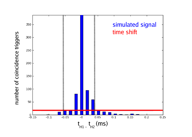
Figure 2.19: A histogram of the number of triggers against the difference in coalescence time $t_{\rm{H1}}-t_{\rm{H2}}$ between H1 and H2. The blue bars represent triggers caused by the software injection of simulated signals and indicate where we might expect to observe triggers caused by true gravitational wave signals (foreground). The red line represent triggers found during analysis of time-shifted data and are used to estimate the non-gravitational wave background. We choose the coincidence windows (vertical dotted lines) so that we will find all the simulated signals that lay above the background in coincidence. Note that the plot shown here only uses nearby injections corresponding to simulated sources with physical distances $50\rm{kpc}<D<500\rm{kpc}$. In order to find simulated sources at larger distances we extended our windows to $\Delta t=100$ms.

Using this tuning method we find our coincidence windows for each detector to have values $\Delta t=100$ ms, $\Delta\psi_{0}=40,000~{}\rm{Hz}^{5/3}$ and $\Delta\psi_{3}=600~{}\rm{Hz}^{2/3}$ (we rounded and symmetrized these values for simplicity). The value of $\Delta t$ used in this search is four times larger than the $25$ ms value used in the S3 search for non-spinning binary black holes [5] indicating that the estimation of arrival time of a gravitational waveform is less well determined in this search than in the non-spinning search.

2.6.7 Combined SNR

We expect rough consistency between the SNR of triggers measured in different LIGO detectors if they originate from the same true gravitational wave signal (or software injected simulated signal) . Conversely, we would not necessarily expect any consistency between the triggers measured in different detectors that are caused by spurious noise events (however, we will see later that seismic activity at the Hanford site can cause triggers in H1 and H2 that are consistent with each other). We assign a combined signal-to-noise ratio $\rho_{c}$ to our coincident triggers based upon the individual signal-to-noise ratios $\rho_{i}$ measured by each detector. For triggers found in coincidence between two detectors we use

$$\rho_{c}^{2}={\rm min}\left\{\sum_{i}^{2}\rho_{\rm i}^{2},(a\rho_{\rm i}-b)^{2}\right\}$$ (2.93)

and for coincident triggers found in all three LIGO detectors we use

$$\rho_{c}^{2}=\sum_{i}^{3}\rho_{\rm i}^{2}.$$ (2.94)

Equation (2.93) assigns higher combined SNR $\rho_{c}$ to coincident triggers with similar SNRs measured in both detectors $\rho_{1}\sim\rho_{2}$ than those consisting of a very loud trigger in one detector and a relatively quiet trigger in the other detector $\rho_{1}\gg\rho_{2}$. In practice the parameters $a$ and $b$ are tuned so that the contours of false alarm generated using Eq. (2.93) separate triggers generated by software injection of simulated signals and background triggers as cleanly as possible [136](see Sec. 2.6.6 for details of how we estimate the background). In this search we used values $a=b=3$ for all detectors. Figure 2.20 shows a scatter plot of the SNR measured in H1 and L1 with lines of constant $\rho_{c}$ (as assigned using Eq. (2.93)). We see that the combined SNR allows us to differentiate between foreground (simulated signals) and background (estimated using time-shifts).

In some cases the presence of a weak (typically H2) trigger would cause the combined SNR of a triple coincidence trigger (using Eq. (2.93)) to be lower than the combined SNR of a double coincidence trigger where the weakest trigger of the triple coincidence has been neglected. This is undesirable since triple coincident triggers are less likely to be caused by noise events than double coincident triggers and we would like to assign triple coincident triggers a higher value of combined SNR to reflect their increased significance. By using Eq. (2.94) to assign the combined SNRs of triple coincident candidates we ensure that the combined SNR of a triple coincident trigger will always be greater than the combined SNR of any two of its constituent triggers would be assigned from Eq. (2.93).

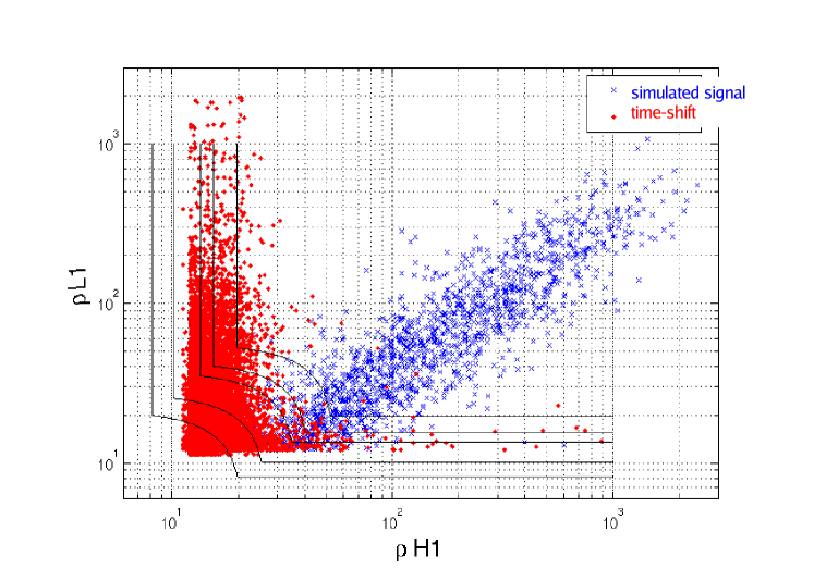
Figure 2.20: Scatter plot of SNR measured in H1 and L1 for H1-L1 coincident triggers occurring in H1-H2-L1 times (i.e., times when all three LIGO detectors were taking science quality data, see Sec. 2.6.3). The blue crosses represent triggers caused by the software injection of simulated signals and indicate where we might expect to observe triggers caused by true gravitational wave signals (foreground). The red dots represent triggers found during analysis of time-shifted data and are used to estimate the non-gravitational wave background. The black curves show contours of constant combined SNR $\rho_{c}$ assigned using Eq. (2.93). Higher values of combined SNR are assigned to coincident triggers caused by simulated signals allowing us to separate these from our estimated background.

2.6.8 Vetoes

Instrument-based vetoes

We are able to veto some background triggers by observing correlation between the gravitational wave channel (AS_Q) of a particular detector and one or more of its auxiliary channels which monitor the local physical environment. Since we would not expect a true gravitational wave signal to excite the auxiliary channels, we will treat as suspicious any excitation in the gravitational wave channel that is coincident in time with excitations in the auxiliary channels. A list of auxiliary channels found to effectively veto spurious (non-gravitational wave coincident triggers) were identified and used for all S3 searches [45]. Additional vetoes based upon other auxiliary channels were considered but were subsequently abandoned because the total amount of data these channels would have discounted, known as the dead-time, was unacceptably large.

Signal-based vetoes

We can use the fact that the Hanford detectors are co-located to veto coincident triggers whose measured amplitude is not consistent between H1 and H2. We check for consistency between the SNR values measured using H1 and H2 data for triggers found in coincidence. Since H1 is the more sensitive instrument we simply required that the SNR measured in H1 be greater than that measured in H2 for an event to survive this veto. Figure 2.21 shows a scatter plot of the SNR measured in H1 and H2 for triggers caused by simulated signals as well as those measured during time-shift analysis with this veto applied. We find that the application of this veto will vastly reduce the number of background triggers but does not affect the number of simulated signals that were observed. Since H1 and H2 were only operated when both were in science mode during S3, this veto means that there will be no H2-L1 coincident triggers since this would indicate that H2 had detected a trigger which H1 was unable to detect.

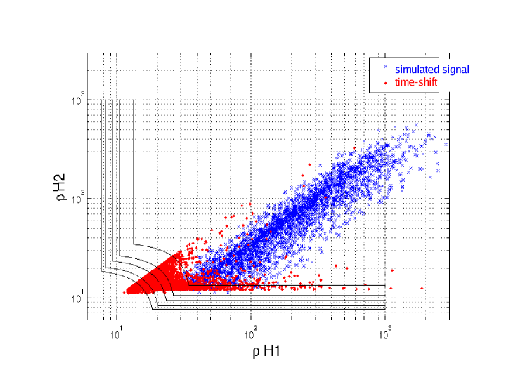
Figure 2.21: Scatter plot of SNR for H1-H2 coincident triggers in H1-H2 times (see caption of Fig. 2.20). We have removed coincident triggers that were measured to have a larger SNR in H2 than in H1. We find that applying this veto vastly reduces the number of background triggers but does not affect the number of simulated signals that were observed.

The $\chi^{2}$ veto used for the primordial black hole and binary neutron star searches [5] has not not been investigated for use in searches using detection template families (i.e., this search and the S2-S4 searches for non-spinning binary black holes [4, 5]).

2.7 Results and follow-up analysis

In the search of the S3 LIGO data described in this paper, no triple-coincident event candidates (exceeding our pre-determined SNR threshold and satisfying the coincidence requirements described in Sec. 2.6.6) were found in triple-time (H1-H2-L1) data. Many double-coincident event candidates were found in both triple-time and double-time (H1-H2) data.

A cumulative histogram of combined SNR for in-time and background coincident triggers is shown in Fig. 2.23. We see that, at the SNR threshold (i.e., the leftmost points on this figure), the number of in-time double-coincident triggers is consistent with the number of coincident triggers yielded by the time-shift analysis. The small excess in the number of in-time H1-H2 coincident triggers at higher SNRs indicates that there is some correlation between the LHO detectors. The coincident triggers contributing to this excess have been investigated and are not believed to be caused by gravitational waves. Seismic activity at the Hanford site has been recorded throughout S3 and can cause data to become noisy simultaneously in H1 and H2. Coincident triggers caused by seismic noise will predominantly cause only in-time coincidences (although time-shift coincidences caused by two seismic events separated in time but shifted together can occur) leading to an excess of in-time coincident triggers as we have observed in Fig. 2.23. As mentioned previously, there were no coincident triggers observed by all three detectors. A scatter plot of the SNRs measured for coincident triggers in H1-H2 times is shown in Fig. 2.24. The distribution of our in-time triggers is consistent with our estimation of the background. This is also true for the double-coincident triggers measured in H1-H2-L1 times.

The loudest in-time coincident trigger was observed in H1-H2 when only the Hanford detectors were in science mode. This event candidate is measured to have SNRs of $119.3$ in H1, $20.4$ in H2 and a combined SNR of $58.3$. The loudest coincident triggers are subjected to systematic follow-up investigations in which a variety of information (e.g., data quality at time of triggers, correlation between the detector’s auxiliary channels and the gravitational wave channel) is used to assess whether the coincident triggers could be confidently claimed as detection of gravitational wave events. This event is found at a time flagged for “conditional” vetoing. This means that during these times some of the detectors auxiliary channels exhibited correlation with the gravitational wave channel (AS_Q ) and that we should be careful in how we treat event candidates found in these times. For this particular coincident trigger an auxiliary channel indicated an increased numbers of dust particles passing through the dark port beam of the interferometer [45]. Upon further investigation it was found that this coincident trigger occurred during a period of seismic activity at the Hanford site and we subsequently discounted this candidate as a potential gravitational wave event. Time-frequency images of the gravitational wave channel around the time of this candidate (see Fig. 2.22) were inconsistent with expectations of what an inspiral signal should look like further reducing the plausibility of this candidate being a true gravitational wave event. It is interesting, but unsurprising, to note that during the search for non-spinning binary black holes that also used S3 LIGO data, high-SNR triggers associated with this seismic activity were also detected [5]. Furthermore, the 20 next loudest event candidates were also investigated and none were found to be plausible gravitational wave event candidates. Work is in progress to automate the follow-up investigative procedure and to include new techniques including null-stream and Markov chain Monte Carlo analysis for assessing the plausibility of coincident triggers as gravitational wave events.

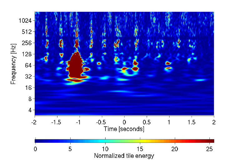
Figure 2.22: Time-frequency image of the gravitational wave channel data taken by H1 about the time of the loudest event candidate, an H1-H2 coincident trigger occurring when only the Hanford detectors were in science mode. A gravitational wave signal would occur at 0 seconds on the time scale of this figure. This figure shows that the H1 gravitational wave channel is noisy at the time of this event and consequently does not improve the likelihood that this candidate was caused by a true gravitational wave signal (see Sec. refsub:results). The H2 gravitational wave channel is also noisy at this time. It is useful to compare this figure with Fig. 2.5 which shows time-frequency maps of the gravitational wave signals observed from inspiraling binaries without the effects of detector noise. This figure was produced using Q Scan [121, 44].

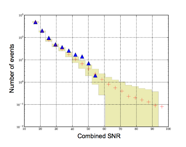
Figure 2.23: Cumulative histograms of the combined SNR, $\rho_{c}$ for in-time coincident triggers (triangles) and our background (crosses with one-sigma deviation shown) for all H1-H2 and H1-H2-L1 times within S3. We see a small excess in the number of in-time coincident triggers with combined SNR $\sim 45$. This excess was investigated and was caused by an excess of H1-H2 coincident triggers. Since H1 and H2 are co-located, both detectors are affected by the same local disturbances (e.g., seismic activity) which contributes to the number of in-time coincidences but which is under-represented in time-shift estimates of the background.

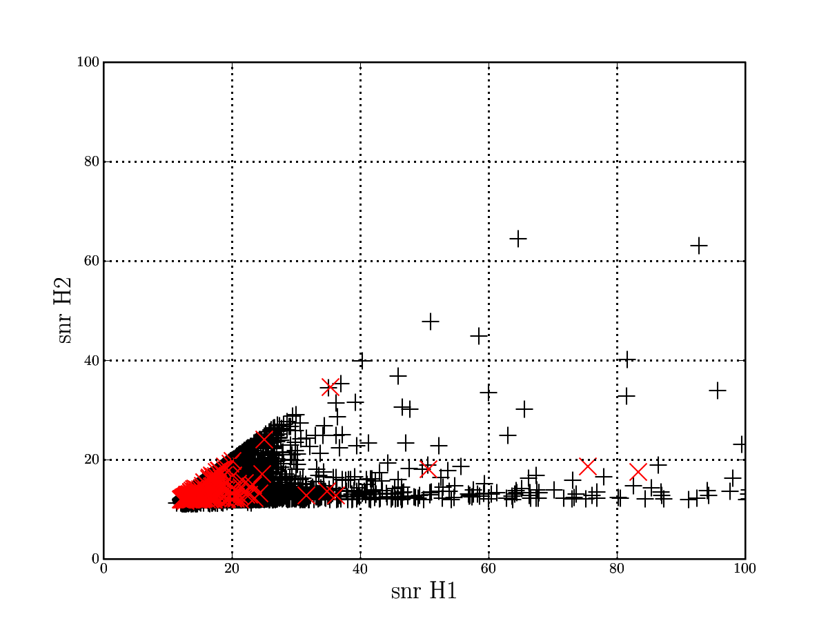
Figure 2.24: Scatter plot of SNR for coincident triggers in H1-H2 times. The light coloured crosses represent in-time coincident triggers and the black pluses represent time-shift coincident triggers that we use to estimate the background. Note that we observe more background triggers than in-time triggers since we perform 100 time-shift analyses to estimate the background but can perform only a single in-time analysis to search for true gravitational wave signals (see Sec. 2.6.6 for further details on background estimation). Note that due to our signal-based veto on H1/H2 SNR we see no coincident triggers with $\rho_{\mathrm{H1}}<\rho_{\mathrm{H2}}$.

2.8 Upper limit on the rate of binary coalescences

Given the absence of plausible detection candidates within the search described above, we calculate an upper limit on the rate of spinning compact object coalescence in the universe. We quote the upper limit rate in units of coalescences per year per $\rm{L}_{10}$ where $\rm{L}_{10}=10^{10}\,\rm{L}_{\odot,B}$ is $10^{10}$ times the blue light luminosity of the Sun.

We assume that binary coalescences only occur in galaxies. The absorption-corrected blue light luminosity of a galaxy infers its massive star formation rate, and therefore supernova rate, which we assume scale with the rate of compact binary coalescence within it [117]. This assumption is well justified when the population of galaxies reached by the detector (i.e., those galaxies which are close enough that it would be possible to detect a stellar mass binary inspiral from within them) is dominated by spiral galaxies with ongoing star formation (e.g., the Milky Way). Papers reporting on S1 and S2  [2, 3, 4] have quoted the upper limit in units of Milky Way Equivalent Galaxy (MWEG) which is equivalent to about $1.7\,\rm{L}_{10}$. Upper limits on the rate of coalescences calculated during other searches using S3 and S4 LIGO are given in units of $\rm{L}_{10}$ [5].

Our primary result will be an upper limit on the rate of coalescence of precessing neutron star - black hole binaries with masses $m_{\rm{NS}}\sim 1.35M_{\odot}$ and $m_{\rm{BH}}\sim 5M_{\odot}$. These mass values correspond to NS-BH binaries with component masses similar to those used to assess the NS-NS and BH-BH upper limits in [5]. We will now detail the calculation of the upper limit on the rate of binary coalescence before applying it to our search of S3 data for systems with spinning components.

The setting of upper limits on rates is discussed in the following publications which were used by the author in writing this Section: Biswas et al. (2007) [23], Brady and Fairhurst (2007) [61] Brady et al. (2004) [33].

2.8.1 Calculating the upper limit

We will treat arrival of a gravitational wave at our detectors as a rare event which can be described by a Poissonian distribution. The probability of detecting no gravitational waves (emitted during binary coalescence) with combined SNR greater than some value $\rho_{c}$ is given by

$$P_{F}(\rho_{c})=e^{-\nu(\rho_{c})}$$ (2.95)

where $\nu(\rho_{c})$ is the mean number of gravitational wave events detected with combined SNR greater than $\rho_{c}$ during the course of a search (e.g., a science run). We can write $\nu$ more explicitly as the product of i) the rate of binary coalescence (per year per $\rm{L}_{10}$), ii) the total (cumulative) luminosity $C_{L}(\rho_{c})$ (in $\rm{L}_{10}$) that the detectors were sensitive to with combined SNR greater than $\rho_{c}$ and iii) the total observation time $T$ (in years). We can therefore write

$$P_{F}(\rho_{c}|R,T)=e^{-R\,T\,C_{L}(\rho_{c})}.$$ (2.96)

The subscript $F$ stands for foreground and is used to distinguish this probability from the probability of measuring a background event with combined SNR greater than $\rho_{c}$ which we shall call $P_{B}(\rho_{c})$.

The probability of measuring no event candidates (true gravitational wave foreground or noise-induced background) with combined SNR greater than that of our loudest observed event candidate $\rho_{c,\rm{max}}$ is given by

$$P(\rho_{c,\rm{max}}|B,R,T) = P_{B}(\rho_{c,\rm{max}})P_{F}(\rho_{c,\rm{max}})$$ (2.97)

$$= P_{B}(\rho_{c,\rm{max}})e^{-R\,T\,C_{L}(\rho_{c,\rm{max}})}.$$

We can calculate the probability density as

$$p(\rho_{c,\rm{max}}|B,R,T) = \frac{d}{d\rho_{c}}P(\rho_{c,\rm{max}}|B,R,T)$$ (2.99)

$$= P_{B}^{\prime}(\rho_{c,\rm{max}})e^{-R\,T\,C_{L}(\rho_{c,\rm{max}})}\times$$

$$\left[1+R\,T\,C_{L}(\rho_{c,\rm{max}})\,\Lambda\right]$$

where we have defined

$$\Lambda=\frac{|\mathcal{C}_{L}^{\prime}(\rho_{c,\rm{max}})|}{P_{B}^{\prime}(\rho_{c,\rm{max}})}\left[\frac{\mathcal{C}_{L}(\rho_{c,\rm{max}})}{P_{B}(\rho_{c,\rm{max}})}\right]^{-1}\,,$$ (2.100)

where the derivatives are with respect to combined SNR $\rho_{c}$. $\Lambda$ is a measure of the likelihood that the loudest event measured during a search is consistent with being a true gravitational wave signal (foreground) rather than being caused by noise (background). We know by definition that the cumulative luminosity $C_{L}(\rho_{c})$ our detectors were sensitive to with combined SNR greater than $\rho_{c}$ will decrease as $\rho_{c}$ increases and therefore that $C_{L}^{\prime}(\rho_{c})$ will always be negative.

Using Bayes’ theorem we can find the posterior probability distribution of the rate $p(R|\rho_{c,\rm{max}},T,B)$ using our prior knowledge or guess of its distribution $p(R)$ and our probability distribution $p(\rho_{c,\rm{max}}|B,R,T)$ for the number of events exceeding the combined SNR of the loudest measured event:

$$p(R|\rho_{c,\rm{max}},T,B)=\frac{p(R)\,p(\rho_{c,\rm{max}}|B,R,T)}{\int p(R)\,p(\rho_{c,\rm{max}}|B,R,T)\,dR}.$$ (2.101)

Since this is the first dedicated search for gravitational waves emitted by binaries with spinning component bodies we have no prior knowledge about the rate. To reflect this, we use a uniform prior, $p(R)=\rm{constant}$. In upper limit calculations for future searches we will be able to use the posterior probability distribution calculated in this search as the prior. Integrating the denominator of Eq. (2.101) by parts yields

$$\int p(R)p(\rho_{c,\rm{max}}|B,R,T)dR$$ (2.102)

$$= P_{B}^{\prime}(\rho_{c,\rm{max}})p(R)\int e^{-R\,T\,C_{L}(\rho_{c,\rm{max}})}\left[1+R\,T\,C_{L}(\rho_{c,\rm{max}})\,\Lambda\right]dR$$

where we can take the prior outside the integral since it is a constant and $P_{B}^{\prime}$ outside the integral since it will clearly not depend on the rate of true gravitational wave events. Evaluating the integrand over all possible rates (from $R=0$ to $R=\infty$) we find

$$\int_{0}^{\infty}p(R)p(\rho_{c,\rm{max}}|B,R,T)dR = P_{B}^{\prime}p(R)\frac{1+\Lambda}{T\,C_{L}}.$$ (2.103)

In practice we can use a finite upper bound on this integral by choosing a large value for the rate $R$ with a suitably low probability of occurring.

Substituting this result back into Bayes’ theorem Eq. (2.101) we find the posterior distribution to be:

$$p(R|\rho_{c,\rm{max}},T,B) = e^{-R\,T\,C_{L}}\frac{T\,C_{L}}{1+\Lambda}\left[1+R\,T\,C_{L}\,\Lambda\right]$$ (2.104)

To find the upper limit $R_{\alpha}$ on the rate of coalescences with confidence $\alpha$ we evaluate

$$\alpha=\int_{0}^{R_{\alpha}}p(R|\rho_{c,\rm{max}},T,B)\,dR.$$ (2.105)

Integrating by parts yields

$$1-\alpha=e^{-R_{\alpha}\,T\,\mathcal{C}_{L}(\rho_{c,\rm{max}})}\left[1+\left(\frac{\Lambda}{1+\Lambda}\right)\,R_{\alpha}\,T\,\mathcal{C}_{L}(\rho_{c,\rm{max}})\right].$$ (2.106)

The corresponding statistical statement would be that we have $\alpha\times 100\%$ confidence that the rate of binary coalescences is less than $R_{\alpha}$.

We evaluate the cumulative luminosity $\mathcal{C}_{L}$ at the combined SNR of the loudest coincident trigger seen in this search, $\rho_{c,\rm{max}}=58.3$ (see Sec. 2.7 for discussion of this coincident trigger).

2.8.2 Observation time

We only use data that was taken during non-playground times in the calculation of the upper limit. The (in-time) non-playground dataset is blinded in the sense that all analysis parameters are tuned and fixed prior to its analysis in order to avoid statistical bias (as described in Sec. 2.6) The observation time $T$ is taken from Table 2.2, where we use the non-playground analysed times.

2.8.3 Calculating the cumulative luminosity

The cumulative luminosity $\mathcal{C}_{L}(\rho_{c})$ to which our search was sensitive to is a function of the detection efficiency of our search $\mathcal{E}$ and the predicted luminosity $L$ of the local universe.

Effective distance and inverse expected SNR

In searches for systems consisting of non-spinning bodies detection efficiency $\mathcal{E}$ is found as a function of its chirp mass $\mathcal{M}=M\eta^{3/5}$ and effective distance which are combined to construct a quantity called the “chirp distance” which describes how detectable a given source is [61, 5]. For low values of chirp distance we would expect high detection efficiency and vice versa. We find that the effective distance is not well defined for a source consisting of spinning bodies and we find an alternative.

For a binary source located at a distance $D$ from a detector, the effective distance $D_{\rm eff}$ is the distance at which it would produce the same SNR if it was positioned directly overhead the detector and with optimal orientation (i.e., face on to the detector, $\iota=0$) [7]. For a system consisting of non-spinning bodies effective distance can be calculated using

$$D_{\rm eff}=\frac{D}{\sqrt{F_{+}^{2}(1+\cos^{2}\iota)^{2}/4+F_{\times}^{2}(\cos\iota)^{2}}}$$ (2.107)

where $D$ is the distance between the binary and the observer, $\iota$ is the inclination angle of the binary with respect to the observer and $F_{+}$ and $F_{\times}$ are the antenna patterns of the detector (see Eq. (2.26)). The effective distance $D_{\rm eff}$ of a binary will always be equal or greater than the physical distance $D$.

For a system consisting of spinning bodies, its inclination $\iota$ with respect to a detector will evolve during the course of the inspiral making the calculation of effective distance complicated (it would in fact be time dependent if we used the formula above). Instead, in this search we find efficiency and predicted source luminosity as a function of the inverse of the expected SNR of a source. The expected SNR is defined as the SNR that would be obtained for a given simulated source assuming we use a template that perfectly matches the emitted gravitational waveform (i.e., fitting factor $=1$) and a detector whose noise power spectrum we can estimate accurately. We therefore define $\rho_{\rm{expected}}=\left<s,h\right>$ where $h$ is our template and $s=Ah$ is our signal. We can calculate the combined expected SNR using the formulae in Sec. 2.6.7.

By taking our distance measure $D_{\rho}$ as the inverse of the expected SNR we obtain a quantity which behaves similarly to the chirp distance by taking larger values for signals which are detectable with a high SNR and by taking smaller values as the signals become less detectable. Since a binary system will have slightly different orientations with respect to the two LIGO observatories, detectors at different sites will measure slightly different expected SNRs and therefore slightly different $D_{\rho}$. We will denote $D_{\rho,\rm{H}}$ as the inverse expected SNR that would be measured at the Hanford site and $D_{\rho,\rm{L}}$ as the inverse expected SNR that would be measured at the Livingston site.

We will find the detection efficiency $\mathcal{E}$ and the luminosity of the nearby universe $L$ both as functions of $D_{\rho,\rm{H}}$ and $D_{\rho,\rm{L}}$ and we need to perform a two-dimensional integration in order to obtain $C_{L}$:

$$\mathcal{C}_{L}(\rho)=\int_{0}^{\infty}\int_{0}^{\infty}\mathcal{E}(D_{\rho,\rm{H}},D_{\rho,\rm{L}},\rho)\,L(D_{\rho,\rm{H}},dD_{\rho,\rm{L}})\,dD_{\rho,\rm{L}}\,dD_{\rho,\rm{H}}.$$ (2.108)

As mentioned earlier, we evaluate $\mathcal{C}_{L}$ at the combined SNR of our loudest event candidate $\rho_{c,\rm{max}}=58.3$.

Detection efficiency

We define detection efficiency as

$$\mathcal{E}(\rho_{c})=\frac{\#_{\rm{found}}(\rho_{c})}{\#_{\rm{found}}(\rho_{c})+\#_{\rm{missed}}(\rho_{c})}$$ (2.109)

where $\#_{\rm{found}}(\rho_{c})$ is the number of simulated signals with combined SNR greater than some $\rho_{c}$ that were detected (found) during the search and similarly $\#_{\rm{missed}}(\rho_{c})$ is the number of simulated signals with combined SNR greater than $\rho_{c}$ that were not detected (missed).

We use software injection of a population of simulated signals (the target waveforms described in Sec. 2.2) to evaluate the detection efficiency $\mathcal{E}$ for observing events with combined SNR greater than $\rho_{c}$, as a function of the source’s inverse expected SNR $D_{\rho}$. In order to sample the parameter space of the binary as thoroughly as possible and to obtain a good estimate of the detection efficiency $\mathcal{E}$ we perform thousands of software injections. We choose the parameters of each binary in our population at random as we described in Sec. 2.6.6 when discussing software injections for the tuning of coincidence windows.

We evaluated the detection efficiency of this search for binaries with component masses distributed uniformly in the range $1.0~{}M_{\odot}<m_{1},m_{2}<20.0~{}M_{\odot}$. During S3, LIGO’s efficiency to binaries in this range was dominated by sources within the Milky Way for which detection efficiency was high across the entire mass range investigated due to the proximity of these sources to Earth. Figure 2.25 shows the detection efficiency measured for recovering software injections in coincidence between H1 and H2 in H1-H2 times against the simulated sources inverse expect SNR.

To calculate the upper limit on the rate of coalescence of NS-BH binaries we will use a Gaussian distribution to generate the component masses of each binary. For the neutron star mass we assume a mean $\mu_{\rm{NS}}=1.35M_{\odot}$ and standard deviation $\sigma_{\rm{NS}}=0.04M_{\odot}$. This choice is motivated by the mass measurements of radio pulsars by Thorsett and Chakrabarty (1999) [139]. Drawing upon analysis of stellar mass black hole observations (Orosz (2002) [106]) and theoretical black hole population studies (Belczynski et al. (2002) [22]), O’Shaughnessy and Kalogera [110] recommend that upper limits on the rate of binary coalescence assume a black hole mass distribution with mean $\mu_{\rm{BH}}=5M_{\odot}$ and standard deviation $\sigma_{\rm{BH}}=1M_{\odot}$. This choice, although slightly ad hoc, corresponds to likely values of BH mass predicted by the population studies in Ref. [110]. Also, by assuming relatively low mass black holes that will appear less luminous to our detector the upper limit we calculate will be correspondingly conservative.

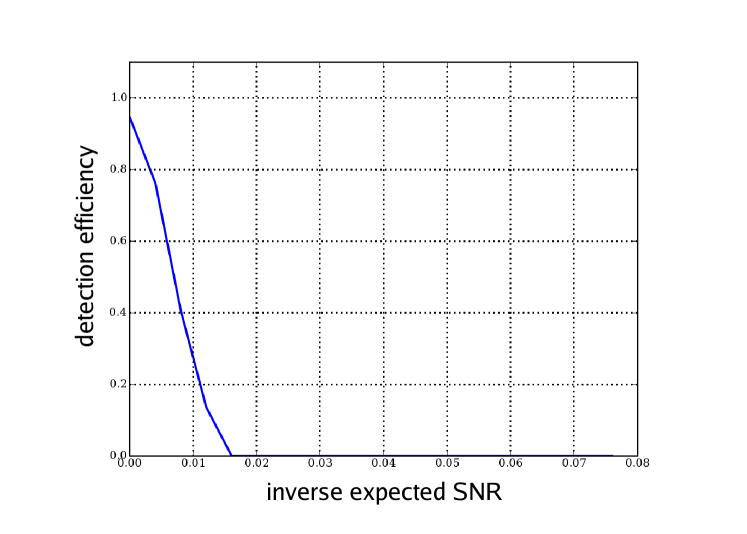
Figure 2.25: Detection efficiency for recovering software injected simulated signals measured against the inverse of the sources expected SNR. This figure contains results for recovering injections in coincidence between H1 and H2 in H1-H2 times only. The reason we only achieve $\sim 95\%$ efficiency at low inverse expected SNR values is because we veto around $5\%$ of H1-H2 times and therefore veto around $5\%$ of our injections which are then subsequently classified as “missed” (see Eq. (2.109)).

Luminosity of the nearby universe

As well as the detection efficiency $\mathcal{E}$ we will also require an estimate of the expected distribution of coalescing binary sources in the nearby universe in order to evaluate the cumulative luminosity $C_{L}$ that our search was sensitive to.

We calculate the luminosity of binary inspirals in the nearby universe by generating a population of simulated signals using information on the observed distribution of sources from standard astronomy catalogues. We use a model based on the work of Kopparapu et al. (2007) [94] for the distribution of blue light luminosity throughout the nearby Universe which we assume is proportional to the rate of binary coalescences (see start of this Section). We will use the same distribution of spins and mass for this population of binaries as we did when assessing the detection efficiency. For each simulated signal we calculate the expected SNR as we did when assessing the efficiency of the search. Figure 2.26 shows the luminosity distribution of the nearby universe.

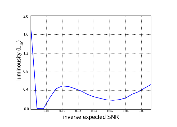
Figure 2.26: Estimated luminosity of the nearby universe against the inverse expected SNR of our simulated sources. Comparing this plot with a similar plot made for the search for black hole binaries with non-spinning components (which had effective distance along the $x$-axis, see Sec. 2.8.3) we are able to find an approximate conversion between inverse expected SNR $D_{\rho,H}$ and effective distance $D_{\rm{eff}}$. We find that $D_{\rm{eff}}\rm{(Mpc)}\simeq 63D_{\rho,H}$. We identify the left most peak on this plot to be caused by the Milky Way, the peak at $D_{\rho,H}\simeq 0.02$ to correspond to Andromeda (M31,NGC0224) and the peak at $D_{\rho,H}\simeq 0.07$ to correspond to Centaurus A (NGC5128).

From our search of S3 data we measure the cumulative luminosity $C_{L}(\rho_{c,\rm{max}})$ and $C_{L}^{\prime}(\rho_{c,\rm{max}})$ for H1-H2 times and H1-H2-L1 times separately. We find

$$C_{L}(\rho_{c,\rm{max,H1-H2}}) = 1.76\,\rm{L}_{10},$$

$$|C_{L}^{\prime}(\rho_{c,\rm{max,H1-H2}})| = 9.2\times 10^{-3}\,\rm{L}_{10}\,\rho_{c}^{\phantom{c}-1},$$

$$C_{L}(\rho_{c,\rm{max,H1-H2-L1}}) = 2.23\,\rm{L}_{10},$$

$$|C_{L}^{\prime}(\rho_{c,\rm{max,H1-H2-L1}})| = 1.5\times 10^{-2}\,\rm{L}_{10}\,\rho_{c}^{\phantom{c}-1}.$$ (2.110)

The averaged values of $C_{L}(\rho_{c,\rm{max}})$ and $C_{L}^{\prime}(\rho_{c,\rm{max}})$ used to calculate the upper limit on the rate (Eq. (2.106)) are simply

$$C_{L}(\rho_{c,\rm{max}}) = \frac{T_{\rm{H1-H2}}\,C_{L}(\rho_{c,\rm{max,H1-H2}})+T_{\rm{H1-H2-L1}}\,C_{L}(\rho_{c,\rm{max,H1-H2-L1}})}{T_{\rm{H1-H2}}+T_{\rm{H1-H2-L1}}},$$

$$C_{L}^{\prime}(\rho_{c,\rm{max}}) = \frac{T_{\rm{H1-H2}}\,C_{L}^{\prime}(\rho_{c,\rm{max,H1-H2}})+T_{\rm{H1-H2-L1}}\,C_{L}^{\prime}(\rho_{c,\rm{max,H1-H2-L1}})}{T_{\rm{H1-H2}}+T_{\rm{H1-H2-L1}}}$$

where $T_{\rm{H1-H2}}$ and $T_{\rm{H1-H2-L1}}$ are the non-playground times listed in Table 2.2.

2.8.4 Background probability

We estimate the background using time-shifts, see Sec. 2.6.6. We estimate the probability $P_{B}(\rho_{c,\rm{max}})$ of there being no background events with combined SNR greater than that of the loudest event as the fraction of time-shift events with combined SNR less than $\rho_{c,\rm{max}}$. Our estimate of the probability density $p_{B}(\rho_{c,\rm{max}})$ is the gradient of $P_{B}(\rho_{c})$ with respect to $\rho_{c}$ at the combined SNR of the loudest event $\rho_{c,\rm{max}}$. For our search of S3 data we estimate $P_{B}(\rho_{c,\rm{max}})=0.23$ and $P_{B}^{\prime}(\rho_{c,\rm{max}})=0.026$.

Combining our results for the background probability $P_{B}$ and cumulative luminosity $C_{L}$ we can find the likelihood (Eq. (2.100)) that the loudest event observed in this S3 was a true gravitational wave event to be  $\Lambda=0.05$ (i.e., 20 times more likely to be caused by noise than a gravitational wave).

We are now in a position to calculate the upper limit on the rate of coalescences of NS-BH binaries. Substituting the values we have calculated for the observation time $T$, the cumulative luminosity $C_{L}$ and the likelihood $\Lambda$ into Eq. (2.106) we obtain the $90\%$ confidence upper limit on the rate to be $R_{90\%}=15.8\,\mathrm{yr}^{-1}\,\mathrm{L_{10}}^{-1}$.

2.8.5 Marginalization of errors

There are a number of systematic uncertainties in this calculation of the upper limit arising from astrophysical and instrumental uncertainties as well as the assumptions we have made during the calculation itself. Systematic errors in the calculated upper limit rate can arise from

• uncertainties in the distances and luminosities of nearby galaxies,

• uncertainties related to the calibration of data recorded by the detectors,

• uncertainties due to the distribution of mass and spins assumed for the population of binaries we use to assess the detection efficiency of our search and the luminosity of the nearby universe,

• uncertainties due to the limited number of software injections we performed in order to assess the detection efficiency and luminosity of the nearby universe.

Note that for searches using different families of matched-filter templates that rely directly upon the modelling of the binary inspiral and the post-Newtonian approximation there is also an uncertainty associated with how well the templates match true gravitational wave signals. However, since we use a detection template family designed to capture a broad range of signals based upon their wave shape (see discussion of detection template families in Sec. 2.3) we ignore this uncertainty.

In order to obtain the most accurate upper limit possible we will marginalize over these uncertainties. This involves specifying a prior distribution that describes how we expect the uncertain parameter to behave. For instance, suppose that our posterior on the rate $p(R|\rho_{c,\rm{max}},T,B,\Lambda)$ depended not only on the combined SNR of the loudest event $\rho_{c,\rm{max}}$, observation time $T$ and our background $B$ but also on some uncertainty in the likelihood $\Lambda$ (due to some uncertainty in $P_{B}$ or $C_{L}$). By assuming a prior distribution $p(\Lambda)$ of the likelihood we would be able to marginalize over this uncertainty using

$$p(R|\rho_{c,\rm{max}},T,B)=\int p(\Lambda)p(R|\rho_{c,\rm{max}},T,B,\Lambda)d\Lambda.$$ (2.111)

The process of marginalization is described further in Biswas et al. (2007) [23] and its application to searches for gravitational waves emitted by binary systems is detailed in Brady and Fairhurst (2007) [61]. After marginalization over these errors we obtain an upper limit of $R_{90\%}=15.9\,\mathrm{yr}^{-1}\,\mathrm{L_{10}}^{-1}$. We also calculate upper limits for a range of binary systems with $m_{1}=1.35M_{\odot}$ and $m_{2}$ uniformly distributed between $2$ and $20M_{\odot}$. These upper limits, both before and after marginalization are shown in Fig. 2.27. These upper limit results are around 7 orders of magnitude larger than the expected rates discussed in Sec. 2.1.1 so do not allow us to constrain the uncertainties in them.

Upper limits on the rate of binaries with non-spinning components

There was no detection of gravitational waves in the S3 and S4 LIGO searches for binaries with non-spinning components and the upper limits on the rate of their coalescence were calculated. The S3 and S4 searches for binaries with non-spinning components are described in Abbott et al. (2007) [5]. We briefly summarise the results of these searches and compare the upper limits on the rates of coalescence calculated.

The S3 search for binary black holes with non-spinning components targeted systems with component masses in the range $3.0M_{\odot}<m_{1},m_{2}<40.0M_{\odot}$. The loudest event candidate observed was in H1 and H2 in H1-H2 times with combined SNR $\rho_{c}=106.5$. We find that this event was the second loudest event observed in the search for binaries with spinning components where it was observed with $\rho_{c}=53.2$ (we identified these events by the GPS time in which their peak SNR was measured). This event was found by the search for binaries with non-spinning components with optimal $\psi_{0}$ and $\psi_{3}$ values well outside the region covered by the search for binaries with spinning components thus explaining the higher SNR it achieved in the non-spinning search. It was noticed that another two of the five loudest event candidates observed in H1-H2 times during the search for asymmetric binaries with spinning components were among the loudest (four) event candidates observed in the search for binary black holes with non-spinning components. In cases where both searches have triggers lying in (or very near) the range of $\psi_{0}$ and $\psi_{3}$ covered by the search for binaries with spinning components we would expect it to yield higher SNR since the BCV2 detection template family used to capture spin-modulated signals has more degrees of freedom (i.e., 6 when $\beta\neq 0$) than the BCV1 detection template family used to capture signals from binaries with non-spinning components.

The upper limit on the rate of coalescence of (approximately symmetric) binary bank holes consisting of non-spinning components with masses distributed with means $m_{\rm{BH}}=5M_{\odot}$ and standard deviations $\sigma_{\rm{BH}}=1M_{\odot}$ was calculated to be $R_{90\%}=23.6\,\mathrm{yr}^{-1}\,\mathrm{L_{10}}^{-1}$. The lack of a $\chi^{2}$ test and the large mass region the search covered lead to the high combined SNR of the loudest event candidate which in turn lead to a comparably high upper limit on the rate of coalescences.

The S3 search for binary neutron stars with non-spinning components targeted systems with component masses in the range $1.0M_{\odot}<m_{1},m_{2}<3.0M_{\odot}$. The upper limit on the rate of coalescence for binary neutrons consisting of non-spinning components with masses distributed with means $m_{\rm{NS}}=1.35M_{\odot}$ and standard deviations $\sigma_{\rm{NS}}=0.04M_{\odot}$ was calculated to be $R_{90\%}=7.97\,\mathrm{yr}^{-1}\,\mathrm{L_{10}}^{-1}$. Again the value of this loudest event can be understood, at least partially, in terms of the loudest event candidate observed in the search which had combined SNR $\rho_{c}\sim 12$. This search utilised a $\chi^{2}$ test and actually used the effective SNR (higher for events that have good $\chi^{2}$ fit to the matched-filter template) to measure the loudness of the events.

The expectation is that we will obtain more interesting (i.e., lower) values for the upper limits on the rates of coalescences in future searches as the sensitivity of the detectors improves leading to larger detection efficiency (and therefore cumulative luminosities $C_{L}$) and improved detector stability leads to longer observation times $T$. This is borne out by the results of the searches of S4 LIGO data for binaries with non-spinning components (B. Abbott et al. (2007) [5]) which yielded $R_{90\%}=0.5\,\mathrm{yr}^{-1}\,\mathrm{L_{10}}^{-1}$ for binary black holes and $R_{90\%}=1.2\,\mathrm{yr}^{-1}\,\mathrm{L_{10}}^{-1}$ for binary neutron stars.

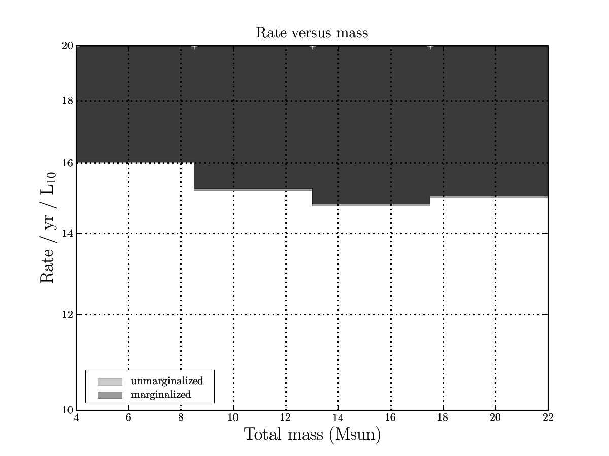
Figure 2.27: Upper limits on the spinning binary coalescence rate per $\mathrm{L}_{10}$ as a function of the total mass of the binary. For this calculation, we have evaluated the efficiency of the search using a population of binary systems with $m_{1}=1.35M_{\odot}$ and $m_{2}$ uniformly distributed between $2$ and $20M_{\odot}$. The darker area on the plot shows the region excluded after marginalization over the estimated systematic errors whereas the lighter region shows the region excluded if these systematic errors are ignored. The effect of marginalization is typically small ($<1\%$). The initial decrease in the upper limit corresponds to the increasing amplitude of the signals as total mass increases. The subsequent increase in upper limit is due to the counter effect that as total mass increases the signals become shorter and have fewer cycles in LIGO’s frequency band of good sensitivity.

Chapter 3 Searching for Extreme Mass Ratio Inspirals using time-frequency algorithms

In this Chapter will turn our attention to the development of data analysis techniques to enable the detection of inspiral events using the planned LISA detector (described in Sec. 1.3.1). We will first describe the various sources LISA is expected to be sensitive to in Sec. 3.1 before reviewing existing data analysis techniques in Sec. 3.2. Having identified the requirement for a computationally cheap method to provide initial detection and rough parameter estimation of LISA sources, in Sec. 3.6 we will detail a time-frequency technique for this purpose, the Hierarchical Algorithm for Clusters and Ridges (HACR). We will then go on to use HACR on a simulated LISA data set and assess its ability to detect gravitational waves from our expected sources.

The analysis described in this Chapter was performed by the author (Gareth Jones) in collaboration with Dr. Jonathan Gair (Institute of Astronomy, University of Cambridge) and has been previously published in Gair and Jones (2007) [85] and Gair and Jones (2007) [86].

3.1 LISA sources

3.1.1 Extreme Mass Ratio Inspirals

Astronomical observations indicate that many galaxies contain a supermassive black hole (SMBH) in its nuclei [57, 113] with masses in the range $\sim 10^{5}-10^{10}M_{\odot}$ [84, 77]. Encounters between bodies in the surrounding star cluster can perturb the orbit of one of those bodies so that its periapse becomes close to the SMBH. The body will radiate energy in the form of gravitational waves and will become bound to the central SMBH. If that body happens to be a compact object such as a white dwarf, neutron star or black hole, it will withstand the tidal forces exerted upon it and will inspiral into the central SMBH. These events are called extreme mass ratio inspirals (EMRIs). The inspiral of compact objects into a SMBH of mass $\sim 10^{5}-10^{7}M_{\odot}$ will emit gravitational waves that we expect to observe with LISA during the final few years before plunge. For a discussion of EMRIs with regard to data analysis, tests of General Relativity and astrophysics see Amaro-Seoane et al. (2007) [8].

The rate at which these extreme mass ratio inspiral (EMRI) events occur in the Universe is highly uncertain, but is likely to be at most only a few times per year in each cubic Gpc of space, see Freitag (2001) [69] and Gair et al. (2004) [71] (see particularly Table 2). LISA EMRI events are thus unlikely to be closer than $~{}1$Gpc, at which distance the typical instantaneous strain amplitude is $h\sim 10^{-22}$ (from Eq. (1) of Wen and Gair (2005) [148] which is similar to Eq. (1.65) of this thesis with the inclusion of the reduced mass $\mu$ in order to take into account the extreme mass asymmetry of these systems). Comparing this value to the characteristic noise strain in the LISA detector of $\sim 5\times 10^{-21}$ at the floor of the noise curve near 5 mHz (see Cutler (1998) [52], Barack and Cutler (2004) [20] and Fig. 1.4) we can see that the instantaneous (rather than accumulated coherent) SNR will be no more than $\sim 0.1$.

3.1.2 Merger of supermassive black holes

LISA should also detect $\sim$ 1-10 signals per year (Sesana et al. (2005) [130], see particularly Fig. 5) from the inspiral and merger of supermassive black hole binaries (SMBHBs) of appropriate mass ($\sim 10^{5}M_{\odot}$ - $10^{7}M_{\odot}$). These events will occur during the merger of the host galaxies of the supermassive black holes and will be visible out to very high redshifts appearing in the LISA data stream with very high signal-to-noise ratio.

3.1.3 Inspiral of white dwarfs

We expect to detect gravitational waves from many millions of compact binaries (composed of white dwarfs (WDs) or neutron stars (NSs)) in the nearby Universe. The orbital shrinkage of these binaries is slow and they generate essentially monochromatic gravitational wave signals (modulo modulation caused by the motion of LISA). At low frequencies the huge number of these binaries will form a confusion foreground, but at higher frequencies we hope to individually resolve several thousands of these binaries (Danzmann et al. (1998) [60], see Fig 1.3 and discussion).

3.2 Data analysis and detection schemes

In this Section we will briefly summarise different methods for the analysis of LISA data in order to detect EMRI signals. We shall see that due to the complexity and duration of these sources matched-filter based analysis will be very computationally expensive (in some cases unfeasible) and we will suggest and subsequently develop a time-frequency based approach.

3.2.1 Matched-filtering for EMRIs

EMRI waveforms will be detectable for several years before plunge, which makes detection possible by building up the signal-to-noise ratio over many waveform cycles using matched filtering as discussed for the inspiral of stellar mass compact objects previously. An EMRI waveform depends on $17$ parameters (although several of these are not important for determining the waveform phasing and we can neglect the spin of the lower mass component) and LISA will detect up to $\sim 10^{5}$ cycles of the waveform prior to plunge. Estimating that one template might be required per cycle in each parameter, and $\sim 6$ important (intrinsic) parameters, gives an estimate of $10^{30}$ templates required for the simplest case of a search for a single EMRI embedded in pure Gaussian noise, this is far more templates than the few $\times 10^{3}-10^{4}$ required in the search for stellar mass spinning systems, see Fig. 2.17. This is far more than can be searched in a reasonable computational time Gair et al. [71].

Markov Chain Monte Carlo techniques

As well as the large number of parameters required to describe an EMRI, the analysis of LISA data is further complicated by the fact that it is signal dominated, i.e., at any moment the data stream includes not only instrumental noise but thousands of signals of different types which overlap in time and frequency. The optimal matched-filter template should, therefore, be a superposition of all the signals that are present. Techniques exist to construct such a global matched filter iteratively, such as Markov Chain Monte Carlo (MCMC) methods, and are currently being investigated in the context of LISA (Cornish and Crowder (2005) [49], Umstätter et al. (2005) [140], Wickham et al. (2006) [150], Cornish and Porter (2007) [50]), including for characterisation of LISA EMRIs [134].

However, even when performed efficiently the MCMC approach still requires the matched-filtering of $\sim 10^{7}$ templates which need to be either generated on the fly or looked up in a template bank. For EMRIs, the computational cost of either approach may be prohibitively high, unless some advance estimate has been made of the parameters of the signals present in the data. To devise such parameter estimation techniques, it is reasonable to first consider the problem of detecting a single source in noisy data, before using and adapting the methods to the case of multiple sources. It is this second problem, searching for a single source while ignoring source confusion, that work on EMRI searches has concentrated on so far.

Semi-coherent matched-filtering for EMRIs

Another possibility for the detection of EMRIs in LISA data is a semi-coherent approach. Rather than search for the full waveform (which may last the majority of LISAs run) we first perform a coherent matched-filter search for $\sim 2-3$ week segments of EMRI waveforms. Subsequently the power in each segment is (incoherently) summed (see e.g., Gair et al. (2004) [71] Sec. 3 for a description of this technique). Assuming reasonable computational resources, this technique could detect individual EMRI events out to a redshift $z\approx 1$ (Gair et al. (2004) [71]), which would mean as many as several hundred EMRI detections over the duration of the LISA mission, although this result is clearly dependent on the intrinsic astrophysical rate of EMRI events. The semi-coherent method, although computationally feasible, makes heavy use of computing resources.

However, the high potential event rate suggests that it might be possible to detect the loudest several EMRI events using much simpler, template-free time-frequency techniques, at a tiny fraction of the computational cost.

3.3 Time-frequency techniques

A promising technique for the detection of EMRIs, and other types of LISA sources, is a time-frequency analysis. We divide the full LISA data set into segments of shorter duration ($\sim 2-3$ weeks) and construct a Fourier spectrum of each, hence creating a time-frequency spectrogram. We then search this time-frequency map for features. The simplest possible time-frequency algorithm is an Excess Power search, where we search the time-frequency map of our data for unusually bright pixels. While Excess Power searches perform poorly when applied to the basic time-frequency map, if the pixels of the time-frequency map are binned first the Excess Power method is able to detect typical EMRI events at distances of up to $\sim 2.25$Gpc (Wen and Gair (2005) [148] and Gair and Wen (2005) [70]) which is about half the distance of the semi-coherent search (Gair et al. (2004) [71]). The disadvantage of the Excess Power method is that it does not by itself provide much information about the source parameters, but merely indicates that a source is present in the data. A follow up analysis must therefore be used to extract information about events identified by the Excess Power search (Wen et al. (2006) [147]).

In this analysis we consider a somewhat more sophisticated time-frequency algorithm, the Hierarchical Algorithm for Clusters and Ridges (HACR) (Heng et al. (2004) [81]). This method involves first identifying unusually bright pixels in the time-frequency map, then constructing a cluster of bright pixels around it, before finally using the number of pixels in the cluster as a threshold to distinguish signals from noise events. The properties of the HACR clusters encode information about the source, and thus in a single analysis HACR allows both detection and parameter estimation.

The HACR search encompasses the Excess Power search as a subset (with the pixel threshold set to 1), which will allow us to compare HACR’s performance to the performance of the Excess Power algorithm in this analysis. We have found that when HACR is applied to the unbinned spectrogram, it performs poorly, but if the spectrogram is first binned via the same technique used for the Excess Power search (Wen and Gair (2005) [148] and Gair and Wen (2005) [70]), we find that HACR outperforms the Excess Power search, as we would expect. HACR is able to detect typical EMRI events at distances of $\sim 2.6$Gpc, which is a little further than the Excess Power technique. However, the HACR clusters associated with detection events tend to have several hundred pixels, and thus encode a significant amount of information about the source. The HACR search can be tuned to be sensitive to a specific source at a specific distance, or to a specific source at an unknown distance, or to an unknown source at an unknown distance. While the detection performance for a specific source does depend on how the HACR thresholds are tuned, we find that the variation of detection rate is not huge and so a single HACR search could be used to detect multiple types of events in a search of the LISA data.

3.4 The LISA data set

The LISA detector was described in Sec. 1.3.4. The main source of noise in LISA is random variations in the frequency of the laser it uses to measure the change in (proper) distance between the spacecraft. However, this laser frequency noise can be suppressed without eradicating the gravitational wave signal through use of Time Delay Interferometry (TDI, see for instance Vallisneri (2005) [141] and references therein). At high frequencies, there are three independent TDI channels in which the noise is uncorrelated which are typically denoted $A$, $E$ and $T$. At low frequencies, there are essentially only two independent data channels since LISA can be regarded as a superposition of two static Michelson ($90^{\circ}$) interferometers at $45^{\circ}$ to each other over the relevant timescales. These two low-frequency response functions, denoted $h_{I}$ and $h_{II}$, are defined in Cutler (1998) [52]. In this analysis we treat the LISA data stream as consisting of only these two channels, since our sources are at comparatively low frequencies, and the responses of the two Michelson interferometers are quick and easy to compute. While not a totally accurate representation of LISA, this approach incorporates the modulations due to the detector motion in a reasonable way and so is sufficient for the qualitative nature of the current analysis.

3.4.1 LISA’s noise spectral density

To characterise the search, we need to include the effects of detector noise. To do this, we use the noise model from Barack and Cutler (2004) [20] , which includes both instrumental noise and “confusion noise” from the unresolvable white dwarf binary foreground. The noise power spectral density is given by

$$S_{h}(f)={\rm min}\left\{S_{h}^{\rm{inst}}(f)\,\exp\left(\kappa T^{-1}_{\rm{mission}}\,dN/df\right),S_{h}^{\rm{inst}}(f)+S_{h}^{\rm{gal}}(f)\right\}$$

$$\hskip 42.67912pt+S_{h}^{\rm{ex.gal}}(f)$$

where $$S_{h}^{\rm{inst}}(f)=9.18\times 10^{-52}\,\,f^{-4}+1.59\times 10^{-41}+9.18\times 10^{-38}\,\,f^{2}{\rm Hz}^{-1}$$

and $$S_{h}^{\rm{gal}}(f)=50\,S_{h}^{\rm{ex.gal}}(f)=2.1\times 10^{-45}\left(\frac{f}{1\,{\rm Hz}}\right)^{-7/3}\,\,{\rm Hz}^{-1}.$$ (3.1)

In this, the parameter $\kappa\,T^{-1}_{\rm{mission}}$ measures how well white dwarfs of similar frequency can be distinguished, and we take $\kappa\,T^{-1}_{\rm{mission}}=1.5/{\rm yr}$ as in Barack and Cutler (2004) [20]. In practice, rather than adding coloured noise to the injected signal, we first whiten the signal using this theoretical noise prescription and then add it to white Gaussian noise. These procedures are equivalent under the assumption that the LISA data stream can be regarded as stationary and supposing that the noise spectral density is known or can be determined. This is likely to be a poor assumption, but a more accurate analysis is difficult and beyond the scope of this project.

3.5 A typical EMRI

In this analysis we concentrate on the issue of detection of EMRI events and to do so we must consider a typical EMRI signal. Work by Gair et al. (2004) [71] using a the semi-coherent search suggested that the LISA EMRI event rate would be dominated by the inspiral of black holes of mass $m\sim 10M_{\odot}$ into SMBHs with mass $M\sim 10^{6}M_{\odot}$. An EMRI will be detectable for the last several years of the inspiral, and hence could last for a significant fraction of the LISA mission duration ($\sim 3-5$ years). Moreover, since the stellar mass black hole will typically be captured with very high eccentricity and random inclination with respect to the equatorial plane of the SMBH, its orbit as it inspirals is likely to have some residual eccentricity and inclination at plunge.

Theoretical models (Volonteri et al. (2005) [143]) and some observational evidence indicate that most astrophysical black holes will have significant spins (see Table 2.1 for a summary of the measured spins of stellar mass black hole binaries). A super massive black hole that has accreted substantial mass via accretion of material with constant angular momentum axis (e.g. a non-precessing disk) would spin up to near the maximal value allowed (i.e. 0.998). A super massive black hole formed by the merger of two objects of comparable mass is expected to have substantial spin whereas a super massive black hole that has accreted mass via capture of low-mass objects from random directions would not accumulate significant spin (see Rees and Volonteri (2007) [123] Sec II and references therein). Since our analysis, Brenneman and Reynolds (2006) [34] analysed XMM-Newton (X-ray) observations of the supermassive black hole (M = $3-6\times 10^{6}M_{\odot}$ from McHardy et al. (2005) [101]) in the centre of galaxy MCG-06-30-15. Their analysis (X-ray spectroscopy) strongly ruled out that the black hole is non-spinning and instead infers a value $\chi\simeq 0.989$.

Bearing all this in mind, we choose as a “typical” EMRI event (which we shall refer to as source “A”) the inspiral of a $10M_{\odot}$ black hole into a $10^{6}M_{\odot}$ SMBH with spin $a=0.8M$. We assume conservatively that the LISA mission will last only three years ($3\times 2^{25}$s) and that the EMRI event is observed for the whole of the LISA mission, but plunges shortly after the end of the observation. This sets the initial orbital pericentre to be at $r_{p}\approx 11M$. We take the eccentricity and orbital inclination at the start of the observation to be $e=0.4$ and $\iota=45^{\circ}$ and fix the sky position in ecliptic coordinates to be $\cos\theta_{S}=0.5$, $\phi_{S}=1$. The orientation of the SMBH spin is chosen such that if the SMBH was at the Solar System Barycentre, the spin would point towards ecliptic coordinates $\cos(\theta_{K})=-0.5$, $\phi_{K}=4$. These latter orientation angles were chosen arbitrarily, but are non-special.

We generate the EMRI waveform using the approximate, “kludge”, approach described in Babak et al. (2007) [18] and Gair and Glampedakis (2006) [72]. These kludge waveforms are much quicker to generate than accurate perturbative waveforms, but capture all the main features of true EMRI waveforms and show remarkable faithfulness when compared to more accurate waveforms.

In addition to source “A”, we will consider two other EMRI injections. These have the same parameters as “A”, except for the initial orbital eccentricity, which is taken to be $e=0$ for source “K” and $e=0.7$ for source “N”. The waveforms and waveform labels used are the same as those examined in the context of the Excess Power search in Gair and Wen (2005) [70] (see Table 1) to facilitate comparison. Figures 3.1 and 3.2 show how these signals can expect to be observed by LISA.

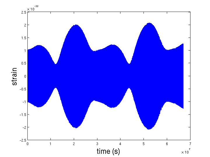
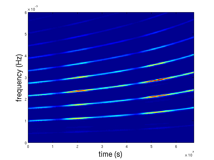
Figure 3.1: Time-series (upper panel) and spectrogram (lower panel) plots of EMRI “A” as it would be observed by LISA. The amplitude modulation of the observed signal due to LISA’s orbit about the sun is clearly visible in these plots. In the spectrogram various harmonics of the fundamental gravitational wave frequency are observed (see caption of Fig. 3.2 for further details). Note the “chirping” nature of the individual tracks on the spectrogram showing the increase of gravitational wave amplitude and frequency as the system evolves.

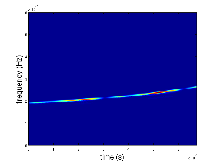
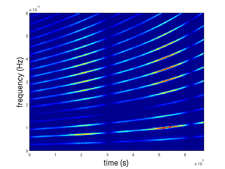
Figure 3.2: Spectrograms of EMRI “K” (upper panel) and “N” (lower panel) as they would be observed by LISA. The splitting of signal power into the different harmonics of the fundamental gravitational wave frequency is a function of the EMRI’s orbital eccentricity $e$. For eccentric orbits, like those of sources “A” and “N” most of the gravitational radiation is emitted at the periapse of the orbit. For more eccentric orbits, these peaks in the emission of gravitational radiation become more concentrated in time than for less eccentric orbits and higher harmonics in the frequency domain are observed (see Sec. III of Peters and Matthews (1964) [116]). Indeed, more harmonics are observed for EMRI “N” ($e=0.7$) than EMRI “A” ($e=0.4$, see Fig. 3.1) or EMRI “K” ($e=0$). Estimation of an EMRI’s parameters using time-frequency representations of an observed signal is described in Wen et al. (2006) [147] and Gair et al. (2007) [73] (see Sec. 3.11). For example, the separation between the time-frequency tracks corresponding to different harmonics can be used to estimate the system’s orbital frequency near peripase. Precession of the system’s orbital plane, discussed in the previous Chapter for stellar mass binaries, will cause splitting of each of the tracks into different sidebands. The separation of these sidebands can be used to estimate the rate of precession of the orbital plane and the orientation of the SMBH’s spin [73].

In Section 3.10, we will examine the performance of HACR in detecting other LISA sources, namely white dwarf binaries and SMBH mergers. For both of these sources, we take the waveform model, including detector modulations, from Cutler (1998) [52]. Although more sophisticated SMBH merger models are available, the prescription in Cutler (1998) [52] is sufficiently accurate for our purposes. The waveform model for a non-evolving white dwarf binary is very simple and has been well understood for many years and is summarised in Cutler (1998) [52].

3.6 The Hierarchical Algorithm for Clusters and Ridges

The HACR algorithm identifies clusters of pixels containing excess power in a time-frequency map (not necessarily a spectrogram) and represents a variation of the TFClusters algorithm described in Sylvestre (2002) [135]. In a given time-frequency map, we denote the power in a pixel as $P_{i,j}$ where $i$ and $j$ are the time and frequency co-ordinates of the pixel. HACR employs two power thresholds, $\eta_{\rm{up}}>\eta_{\rm{low}}$ and a threshold on the number of pixels above the power thresholds, $N_{p}$. At the first stage, the algorithm identifies all black pixels with $P_{i,j}>\eta_{\rm{up}}$ and all grey pixels with $P_{i,j}>\eta_{\rm{low}}$. At the second stage, HACR takes each black pixel in turn and counts all the grey pixels that are connected to that black pixel through a path of touching grey pixels. Touching is defined as sharing an edge or corner. This process is repeated for each black pixel. To be classified as an event candidate a cluster of pixels must have $N_{c}>N_{p}$ where $N_{c}$ is the number of pixels contained in a particular cluster. The algorithm is illustrated in Fig. 3.3.

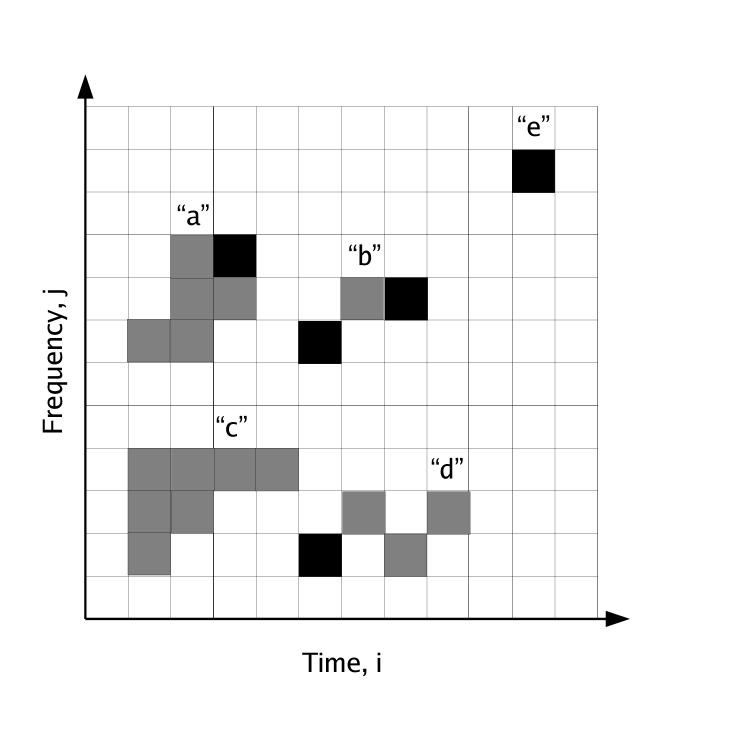
Figure 3.3: A simple time-frequency map illustrating properties of the HACR algorithm. Pixels with power $P_{i,j}>\eta_{\rm{up}}$ are classified as black pixels. Surrounding pixels with $P_{i,j}>\eta_{\rm{low}}$ are then classified as grey pixels building a cluster around the black pixel. The cluster is classified as an event candidate if the number of pixels it contains, $N_{c}$, exceeds the threshold $N_{p}.$ Assuming $N_{p}<6$ we would classify cluster “a” as an event candidate. Clusters (“b”) may contain more than more black pixel (or even consist solely of black pixels) but still require $N_{c}>N_{p}$ to be classified an event candidate. Clusters of any size (“c”) require at least one black pixel to be classified an event candidate. Pixels connected by their corners (“d”) only still count as connected. In the limit $N_{p}=1$ HACR will mimic a simple Excess Power search identifying all black pixels as event candidates (e.g., “e”).

There is some degeneracy between the thresholds, particularly $\eta_{\rm{low}}$ and $N_{p}$. Choosing a low value of $\eta_{\rm{low}}$ tends to make clusters larger but we can limit the number of these clusters which become an event candidate by using a larger value for the pixel threshold, $N_{p}$. In our preliminary analysis, we fixed the value of $\eta_{\rm{low}}$ and tuned only $N_{p}$. However, tuning $\eta_{\rm{low}}$ as well can enhance the detection rate by $10-15\%$. The results shown in this analysis use tuning over both thresholds. The thresholds affect not only the detection rate, but also parameter extraction. Reducing $\eta_{\rm{low}}$ in order to make clusters larger might increase the detection rate, but it will also increase the number of noise pixels in each event candidate which will hamper parameter extraction. The optimal thresholds for the final search will ultimately come from a compromise between greater reach and more accurate parameter extraction. In a future paper, when we explore parameter estimation, we will examine this issue more carefully. In the current analysis, we look only at maximizing the detection rate.

3.6.1 Investigating binning of the time-frequency maps

It is possible to improve the performance of the search by “binning” the time-frequency maps. This binning procedure was the key stage in the simple Excess Power search discussed in Wen and Gair (2005) [148] and Gair and Wen (2005) [70].

This binning procedure involves constructing an average power map using boxes of a particular size. The average power contained within a box is defined by

$$P_{i,j}^{n,l}=\frac{1}{m}\,\sum^{n-1}_{a=0}\sum^{l-1}_{b=0}P_{i+a,j+b}$$ (3.2)

where $n$, $l$ are the lengths of the box edges in the time and frequency dimensions respectively, and $m=n\times l$ is the number of data points enclosed. This average power is computed for a box aligned on each pixel in the (original unbinned) time-frequency map. Adjacent pixels in the binned time-frequency map are therefore not independent. In practice, for ease of computation we choose the alignment so that the pixel we use to label each box is in the top left hand corner of that particular box. As in Wen and Gair (2005) [148], we use only box sizes $(n,l)=(2^{n_{t}},2^{n_{f}})$ for all possible integer values of $n_{t}$ and $n_{f}$. We denote the total number of different box shapes used as $N_{\rm{box}}$.

For a given source, the box size that will do best for detection will be large enough to include much of the signal power but small enough to avoid too much contribution from noise. This optimum will be source specific due to the wide variation in waveforms. The inspiral of a $0.6M_{\odot}$ white dwarf occurs much more slowly than that of a $10M_{\odot}$ black hole, so in the first case, the optimal box size is likely to be longer in the time dimension. Gravitational waves from an inspiral of a compact object into a rapidly spinning black hole or from a highly eccentric inspiral orbit are characterised by many (often closely packed) frequency harmonics. In this case, a box that is wider in the frequency dimension may perform well. In designing a search, a balance must therefore be struck between having sensitivity to a range of sources and increasing the reach of the search for a specific source. We will consider this more carefully in Sec. 3.9.

Efficient “binning” method

The binned spectrograms for each box size can be generated in a particular sequence that improves the efficiency and speed of the search as shown in Figure 3.4. We first construct the unbinned $(n=1,l=1)$ map of the data and store it as map A. Before analysing map A we construct the $(n=1,l=2)$ map by summing the powers in vertically adjacent pixels and storing this as map B (step 1). We then search map A using HACR before summing the power of pixels in horizontally adjacent pixels to construct the $(n=2,l=1)$ map, and overwrite map A (step 2). Repeating this procedure on this new map A, we construct and search all the box sizes $(n=2^{n_{t}},l=1)$. Before analysing the $(n=1,l=2)$ map stored as map B we construct the $(n=1,l=4)$ map and store this as map A (step 3). Using and overwriting map B, we construct and search all the box sizes $(n=2^{n_{t}},l=2)$ (step 4). We repeat this procedure until we have searched all possible box sizes up to the limit imposed by the size of our time-frequency map.

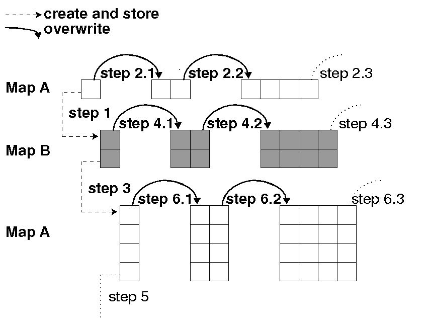
Figure 3.4: A schematic showing how we bin the pixels of our time-frequency map in an efficient manner following the algorithm described in Sec. 3.6.1. This Figure was designed by Gair and Jones for [85] and was drawn by Gair.

This efficient binning method requires the storage of only two time-frequency maps at any given time and reduces the number of floating point operations needed through careful recycling of maps. It is therefore very computationally efficient.

We set the HACR thresholds separately for each binned time-frequency map and label them according to the dimensions of the box they are tuned for, i.e., $\eta_{\rm{low}}^{n,l}$, $\eta_{\rm{up}}^{n,l}$ and $N_{p}^{n,l}$. A HACR detection occurs if there is an event candidate (i.e., a cluster satisfying our thresholds) in at least one binned time-frequency map.

To characterise the entire search (over all box sizes) we define an overall false alarm probability ($OFAP$). This is defined as the fraction of LISA missions in which HACR would make at least one false detection in at least one of the binned time-frequency maps in the absence of any gravitational wave signals. Each box size that we use to analyse the data could be allowed to contribute a different amount to $OFAP$, but to avoid prejudicing our results, we choose to assign an equal false alarm probability to each box size. We call this quantity the additional false alarm probability ($AFAP$). To be clear, $AFAP$ is the probability of a false alarm in a time-frequency map with a particular box size, i.e., the fraction of LISA missions in which that particular box size would yield a false detection. The way in which the thresholds are computed ensures that time-frequency maps with each box size adds $AFAP$ to the overall false alarm rate (hence “additional”), despite the fact that the binned time-frequency maps are not all independent. This will be described in Sec. 3.8.1, and ensures that in practice $OFAP=N_{\rm{box}}\times AFAP$.

It is important to note that in the case $N_{p}=1$ then the HACR algorithm is equivalent to the Excess Power method described in earlier papers Wen and Gair (2005) [148] and Gair and Wen (2005) [70]. A comparison between these two algorithms will be made in subsequent Sections of this thesis.

3.6.2 Constructing spectrograms

We consider a three year LISA mission, and used $T_{\rm{LISA}}=3\times 2^{25}$ seconds of simulated LISA data sampled at $f_{s}=0.125$ Hz (a cadence of $\Delta t=8$ seconds). To construct the time-frequency map, we divided our time series data into $T_{\rm{segment}}=2^{20}$ seconds ($\sim 2$ week) time segments and an FFT was performed on each segment. The frequency resolution of the spectrogram is $\Delta f=1/T_{\rm{segment}}$. The highest frequency we can sample without suffering low frequency aliasing is determined by the frequency at which we sample our continuous stream of data, $f_{s}$. The Shannon-Nyquist sampling theorem states that we can exactly reconstruct the original continuous stream of data from our sampled data set as long as the original data stream is band limited to contain only frequencies less than half the sampling frequency. This critical frequency is known as the Nyquist frequency, $f_{\rm{Nyquist}}=0.5f_{s}$. Figure 3.5 shows how the various quantities described above define the resulting spectrogram. The resulting time-frequency spectrograms consist of $96$ points in time and $65536$ points in frequency giving us $N_{\rm{box}}=7\times 17=119$ possible box sizes of the form $n=2^{n_{t}},l=2^{n_{f}}$ where $n_{t}=0\dots 6$ and $n_{f}=0\dots 16$. Note that we do not use box size $(n=2^{6},l=2^{16})$ since in this case our entire spectrogram will be represented by only a single box.

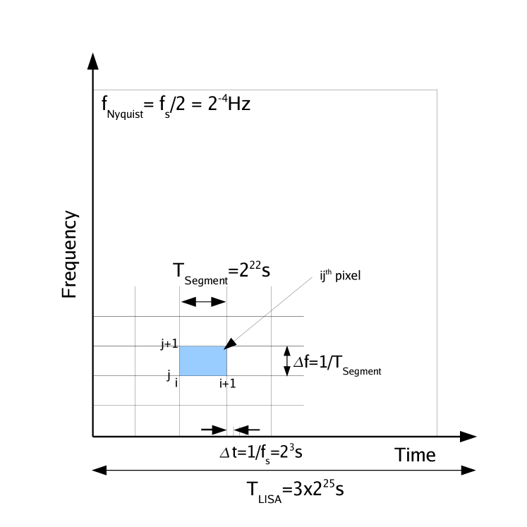
Figure 3.5: Schematic diagram describing the construction of a spectrogram. The LISA data set, length $T_{\rm{LISA}}$ is divided into $N_{\rm{segment}}$ time segments of length $T_{\rm{segment}}$. The data stream is sampled at $f_{s}=0.125$ Hz which corresponds to a cadence of $\Delta t=8$ seconds. Each segment will contain $N_{\rm{sample}}$ samples, i.e., $T_{\rm{segment}}=N_{\rm{sample}}\Delta t$. We have frequency resolution $\Delta f=1/T_{\rm{segment}}$ the maximum frequency we can sample without aliasing is $f_{\rm{Nyquist}}=0.5f_{s}$. We will therefore have $N_{\rm{samples}}$ frequency bins in our spectrogram.

A power spectrogram was constructed separately for both LISA low-frequency channels, $h_{I}$ and $h_{II}$ and these were summed pixel by pixel to produce the time-frequency map searched by the HACR algorithm. The power in the $ij^{th}$ pixel of the time-frequency map searched by HACR is given by

$$P_{i,j}=\sum_{\alpha=I,II}\left[\frac{2|\tilde{h}_{\alpha,i,j}+\tilde{n}_{\alpha,i,j}|^{2}}{\sigma^{2}_{\alpha,j}}\right],$$ (3.3)

where we have written our data in the Fourier domain as $\tilde{x}=\tilde{h}+\tilde{n}$ (where $h$ is a signal and $n$ is noise) and $\sigma^{2}$ is the expected variance of the noise component $n_{j}$. This is given by

$$\sigma^{2}_{j}=\frac{S_{h}(f)}{2(\Delta t)^{2}\Delta f}.$$ (3.4)

In practice, the noise in the two LISA channels was taken to be Gaussian and white and the injected signals were whitened using the theoretical LISA noise curve $S_{h}(f)$ described in Sec. 3.4.1. In this approach, in the absence of a signal the power, $P_{i,j}$, in each pixel of the unbinned spectrogram will be distributed as a $\chi^{2}$ with 4 degrees of freedom.

The division into $\sim 2$ week segments was chosen to facilitate comparison with the Excess Power search (Wen and Gair (2005) [148] and Gair and Wen [70]), and it is a fairly reasonable choice for EMRIs. We would ideally like to ensure that the power measured in the spectrogram corresponding to a particular gravitational wave signal (e.g., a given harmonic of an inspiral chirp) is not split into too many small clusters. The maximum segment length that ensures a source whose frequency is changing at $df/dt$ does not move by more than one frequency bin over the duration of the segment (i.e., $df/dt=\Delta f/T_{\rm{segment}}$) is $T_{\rm{segment}}=1/\sqrt{df/dt}$. In the extreme mass ratio limit, the leading order post-Newtonian rate of change of frequency is

$$\frac{df}{dt}=\frac{192}{5}\frac{m}{M^{3}}\left(\frac{M}{r}\right)^{11/2}$$ (3.5)

for a circular orbit of radius $r$ (in units with $c=G=1$) (use Eq. (5.6) of Peters (1964) [115] for $dr/dt$ with Kepler’s third law). For the inspiral of a $m=10M_{\odot}$ object into a $M=10^{6}M_{\odot}$ this gives a maximum segment length of $\sim 1$ day when the orbital radius is $r=10M$. At that radius, the frequency would change by $\sim 10$ bins during one $2$ week time segment. This change is less rapid earlier in the inspiral and more rapid later in the inspiral. If we choose time segments that are too short, the spectrogram will be dominated by short timescale fluctuations in the detector noise, and the frequency bins will be broad, so we lose resolution in the time frequency map. Time segments with length $\sim 1$ week seem like a reasonable compromise. In the future, we plan to experiment with shorter and longer time segments. However, the choice of time segment length should not significantly affect our results thanks to the binning part of the search algorithm.

3.6.3 Computational cost of a HACR search

The computational cost of running the HACR search is very low. We divide the LISA data stream ($T_{\rm{LISA}}$) into $N_{\rm{segments}}$ time segments of length $T_{\rm{segment}}$. Each time segment contains $N_{\rm{samples}}$ time samples. To FFT one time segment we perform $\sim N_{\rm{samples}}\log N_{\rm{samples}}$ floating point operations. Therefore, to construct spectrograms for the full LISA data stream ($N_{\rm{segments}}$) for both channels, $h_{I}$ and $h_{II}$, must perform $\sim 2N_{\rm{segments}}N_{\rm{samples}}\log N_{\rm{samples}}$ operations.

The efficient binning algorithm ensures that only two floating point operations are needed to evaluate the average power for a given pixel in any one of the binned spectrograms (as opposed to $n\times l+1$ operations if the binned spectrogram was computed directly from the unbinned map). Our unbinned spectrogram will have $N_{\rm{segment}}$ points in the time and $N_{\rm{sample}}$ points in frequency. The number of operations required to construct all the binned spectrograms is therefore less than $N_{\rm{segments}}N_{\rm{samples}}\log_{2}N_{\rm{segments}}\log_{2}N_{\rm{samples}}$ (less since the average power is not defined for pixels in the last $n-1$ columns and $l-1$ rows when using the $n\times l$ box size).

The HACR algorithm first identifies pixels as black, grey or neither ($N_{\rm{segments}}N_{\rm{samples}}$ operations) and then counts the number of pixels in each cluster. For a given cluster, counting the size involves $9$ operations per pixel ($8$ comparisons to see if the 8 possible neighbours are also in the cluster and one addition to increment pixel count $N_{p}$). If HACR has identified $N_{c}$ clusters, and cluster $c_{j}$ has $N_{p}(c_{j})$ pixels, this makes $N_{c}(9N_{p}(c_{j})+1)$ operations in total, assuming no overlap between the clusters. We do not know in advance how many clusters HACR will identify, nor how many pixels will be in each one. However, we know that we cannot have more clusters than pixels $N_{c}<N_{\rm{segments}}\,N_{\rm{samples}}$. We also limit the number of pixels in a cluster to $N_{p}<50000$ by choosing the minimal lower power threshold $\eta_{\rm{low}}$ (this will be described in the Sec. 3.7).

In practice, to run the HACR search with a single set of tuned thresholds on a spectrogram containing a single source, and with LISA and box size parameters as described in Sec. 3.6.2, takes about $1$ minute on a $3.5$GHz workstation. If more sources were present, this time would be larger since more clusters would be identified, but $10$ minutes would be an upper limit. This should be compared to the cost of the semi-coherent search which requires $\sim 3$ years on a $50$Tflops cluster (Gair et al. (2004) [71]). It should be noted that noise characterisation and tuning of HACR is more expensive, since it involves using low thresholds (thus increasing the number of HACR clusters identified), and repeating over many noise realisations. However, to complete $1000$ tuning runs using $40$ nodes of a typical computer cluster still takes only a few hours.

3.7 Searching characterisation

Tuning HACR is a two step process. Firstly, simulated noisy data is analysed in order to identify triplets of our thresholds $\eta^{n,l}_{low}$, $\eta^{n,l}_{up}$ and $N^{n,l}_{p}$ which yields a specified false alarm probability $AFAP$ for each box size $n\times l$. Secondly, a stretch of simulated data containing both noise and a signal is analysed using these threshold triplets and the detection rate (or detection probability) is measured. For each value of false alarm probability considered we can then choose the threshold triplet that gives the largest detection rate. In this way, we obtain the optimal Receiver Operating Characteristic (ROC) curve for the detection of a particular source.

We will use the terms detection rate and false alarm probability in order to make a distinction between event candidates caused by a signal or by noise. What we are really computing as the detection rate is the detection probability, i.e., the fraction of LISA missions in which a particular source would be detected if we had many realisations of LISA. A more relevant observational quantity is the fraction of sources of a given type in the Universe that would be detected in a single LISA observation. The population of LISA events will have random sky positions, plunge times and plunge frequencies. They therefore sample different parts of the time-frequency spectrogram, which to some extent mimics averaging over noise realisations. The detection rate can thus be taken as a guide to the fraction of sources similar to the given one that would be detected in the LISA mission. A more accurate assessment of the fraction of sources detected requires injection of multiple identical sources simultaneously, but we do not consider that problem here.

To characterise the noise properties of the search we used $10000$ noise realisations and analysed them for twenty choices of $\eta_{\rm{low}}^{n,l}$ and with the threshold $\eta_{\rm{up}}^{n,l}$ set as low as is sensibly possible, recording the peak power, $P_{\rm{max}}$, and size, $N_{c}$, of every cluster detected. With such a list of clusters, it is possible during post-processing (discussed in Sec. 3.7.1) to obtain the number of false alarm detections that would be made using any of the twenty lower thresholds, $\eta_{\rm{low}}$, any value of $\eta_{\rm{up}}>(\eta_{\rm{up}}^{n,l})_{\rm{min}}$ and any value of $N_{p}$. The value of $(\eta^{n,l}_{\rm{up}})_{\rm{min}}$ has to be chosen carefully. If it is too low, many clusters will be found in every noise realisation, increasing the computational cost. If it is too high, too few clusters will be identified to give reasonable statistics. We used values of $(\eta^{n,l}_{\rm{up}})_{\rm{min}}$ chosen to ensure that a few clusters were found for each box size in each noise realisation. The lower threshold has to be less than or equal to $(\eta^{n,l}_{\rm{up}})_{\rm{min}}$. If it is set too low, large portions of the time-frequency map can be identified as a single cluster. Therefore, we choose the minimum value of $\eta_{\rm{low}}^{n,l}$ to ensure that all clusters are of reasonable size, which we define to be less than $50000$ pixels. By examining cluster properties in a few thousand noise realisations, we found suitable empirical choices to be

$$\alpha^{n,l} = 4+\frac{10\sqrt{2}}{(nl)^{5/9}}$$ (3.6)

$$(\eta_{\rm{low}}^{n,l})_{\rm{min}} = 4+4\sqrt{\frac{10}{50000+nl}}$$ (3.7)

$$(\eta_{\rm{up}}^{n,l})_{\rm{min}} = \rm{max}[\alpha^{n,l},(\eta_{\rm{low}}^{n,l})_{\rm{min}}].$$ (3.8)

We note that for large box sizes, $\alpha^{n,l}<(\eta^{n,l}_{\rm{low}})_{\rm{min}}$ and so we set $\eta_{\rm{up}}^{n,l}=\eta_{\rm{low}}^{n,l}$. Above this point, we no longer ensure that at least one cluster is found for each box size, as this is inconsistent with the more important requirement that no cluster exceeds $50000$ pixels. We emphasise that our search is robust to the somewhat arbitrary choice of these minimal values. For box sizes where $(\eta_{\rm{low}})_{\rm{min}}<(\eta_{\rm{up}})_{\rm{min}}$, we use 20 values of $\eta_{\rm{low}}$ spaced evenly between $(\eta_{\rm{low}})_{\rm{min}}$ and $(\eta_{\rm{up}})_{\rm{min}}$. Where $(\eta_{\rm{low}})_{\rm{min}}=(\eta_{\rm{up}})_{\rm{min}}$ we use only one lower threshold $\eta_{\rm{low}}=(\eta_{\rm{up}})_{\rm{min}}$. This comparatively small number of lower threshold choices is sufficient to find the maximum detection rate thanks to the degeneracy between $N_{p}$ and $\eta_{\rm{low}}$ mentioned earlier.

3.7.1 Post-processing

For each box size and each lower threshold value we can consider values of $\eta_{\rm{up}}^{n,l}$ between $(\eta_{\rm{up}}^{n,l})_{\rm{min}}$ and the maximum power measured $(\eta_{\rm{up}}^{n,l})_{\rm{max}}$, and construct a list of all clusters with peak power $P_{\rm{max}}>\eta_{\rm{up}}^{n,l}$, ordered by increasing number of pixels $N_{c}$.

If we have set the false alarm rate of each box size to be $AFAP$, we expect to see $N_{\rm{rls}}\times AFAP$ false alarms in $N_{\rm{rls}}$ noise realisations. By looking at the list of clusters, we can identify a value of the threshold $N_{p}^{n,l}$ with each pair of values for $\eta_{\rm{up}}^{n,l}$ and $\eta^{n,l}_{\rm{low}}$ that would give the correct number of false alarms in the realisations considered. If HACR was used to analyse pure noise with those three thresholds and only one box size $(n,l)$, it would yield a detection rate $AFAP$. A typical relationship between $\eta_{\rm{up}}^{n,l}$ and $N_{p}^{n,l}$ for a fixed choice of $\eta_{\rm{low}}^{n,l}$ is shown in the upper panel of Figure 3.6. This was generated for a box size $n=1$, $l=64$, the $6$th lower threshold value of the $20$ examined, and for three choices of $AFAP=0.01,0.005$ and $0.0025$.

Figure 3.6: Upper panel: Contours of constant (additional) false alarm probability $AFAP$ for the box size $n=1,l=64$ and one particular lower threshold value. Pairs of thresholds $\eta_{\rm{up}}$ and $N_{p}$ which lie on a contour yield the same additional false alarm probability. Lower panel: Rate of signal detection plotted against choice of threshold, again for fixed lower threshold. Each point on the $x$-axis represents a set of thresholds which yield a particular value of $AFAP$. By choosing the threshold set which yields the largest value of detection rate, plotted on the $y$-axis, we can maximise the rate of signal detection for a given false alarm probability.

To determine which combination of thresholds is optimal, we subsequently analyse spectrograms containing both noise and an injected signal. As mentioned earlier, since we are using white noise to generate the noise realisations, the signal is first whitened using the noise model described in Sec. 3.4.1 before injection. For each box size we may then select the triplet of thresholds which yields the largest detection rate. The lower panel of Fig. 3.6 shows detection rate plotted against upper threshold value for EMRI source “A” at a distance of 2Gpc using the box size $n=1$, $l=64$ with $AFAP=0.01,0.005$ and $0.0025$ and for a fixed lower threshold value (the $6$th of the $20$ values used). Although only the $\eta_{\rm{up}}$ threshold value is shown a corresponding value of $N_{p}$ is inferred, determined by the assigned $AFAP$. This stage of the analysis will be discussed further in the next Section.

The full search uses multiple box sizes, searched in a particular order. We want the thresholds in a given box size to contribute an additional false alarm rate of $AFAP$. When determining the threshold triplets we therefore need to ignore realisations in which false alarms have already been found. The procedure above is thus slightly modified when considering more than one box size. If we are using $N_{\rm{rls}}$ noise realisations to determine the thresholds, each box size should give $N_{\rm{rls}}\times AFAP$ false alarms. The necessary threshold triplet can be determined for the first box size as described above. It is then possible to identify the realisations in which the false alarms were found for the first box size. This set of realisations will be somewhat different for each of the triplets of thresholds that give the desired $AFAP$. So, in practice we must do this in conjunction with the source tuning described in the next Section. This allows us to identify an optimal threshold triplet and we can find the noise realisations in which that threshold triplet gave false alarms. We then repeat the procedure described above, but now considering only clusters identified in the remaining realisations. This process is repeated for each box size in turn, ignoring in each subsequent box size any realisations in which false alarms have been identified in earlier box sizes. This means that the order in which the different box sizes are searched affects the thresholds. However, our results show that it does not matter in which order the box sizes are searched, provided the order is the same for tuning and the actual search. This will be discussed further in Sec. 3.8.1.

3.8 Performance of HACR in EMRI detection

3.8.1 Tuning HACR for a single specific EMRI source

The fact that HACR has three thresholds allows the search to be tuned to optimally detect a specific source at a specific distance. For a given choice of false alarm probability, $AFAP$, we can choose triplet of thresholds for each box size $\eta_{\rm{low}}^{n,l}$, $\eta_{\rm{up}}^{n,l}$ and $N_{p}^{n,l}$ that maximises the detection rate. For this optimal threshold triplet, a Receiver Operating Characteristic (ROC) curve can be plotted for the HACR search tuned for that source. The ROC curve shows the detection rate as a function of the overall false alarm probability, $OFAP$, of the search using all box sizes.

In practice, the ROC is determined by generating a sequence of noise realisations, injecting the whitened signal into each one, and then constructing and searching the binned spectrograms. A detection is defined as any realisation in which all thresholds are exceeded in at least one box size. The box sizes are searched in the order they were constructed (see Fig. 3.4). As discussed in the previous Section, if a detection has been made for one box size, we want to ignore that realisation when we search with subsequent box sizes. This ensures that we always choose the threshold triplet for a box size that provides the maximum number of additional detections. In practice, we achieve this goal using the following algorithm

• Search all realisations using the first box size, for threshold triplets (typically $\sim 100$ upper thresholds and $20$ lower thresholds) that all yield the assigned $AFAP$ (obtained through tuning of the pixel threshold).

• Choose the threshold triplet that yields the highest detection rate. Identify every realisation in which this optimal threshold triplet gives a detection.

• Move onto the second box size and repeat this procedure, but only search realisations in which the optimal threshold triplet for the first box size did not yield any detection.

• Repeat for all other box sizes in order.

Once the optimal threshold triplets have been determined in this way, the detection rate must be measured by using these optimal thresholds to search a separate set of signal injections, to avoid biasing the rates. We experimented with using different numbers of injections and concluded that using 1000 signal injections to determine the thresholds and another 1000 signal injections to measure the rate gave reliable answers. We estimate the error in the resulting ROC curve due to noise fluctuations to be less than $3\%$. All the results in this paper are computed in this way. To characterise the noise, we use the same set of 10000 pure noise realisations in all calculations.

In Fig. 3.7 we show the ROC curves for detection of source “A” at a range of distances using HACR. The random search line on this Figure represents a search for which the detection rate and false alarm rate are equal. This is the “random limit” since it is equivalent to tossing a coin and saying that if it is heads the data stream contains a signal and if it is tails it does not. A search that yields a ROC curve equal to this random line is essentially insensitive to signals. In Fig. 3.7, we see that the source has very nearly $100\%$ detection rate for all $OFAP$s explored out to a distance of $\sim 1.8$Gpc. An overall false alarm probability of 10% is probably quite a conservative value, since this is the probability that in a given LISA mission the entire HACR search would yield just a single false alarm. At a distance of 2Gpc, with the overall false alarm probability set to $10\%$, HACR achieves a detection rate of $\sim 90\%$. As the distance increases further, the detection rate further degrades, and the source becomes undetectable at a distance of $\sim 3$Gpc. The rate of EMRI events is somewhat uncertain, but the range for a $10M_{\odot}$ black hole falling into a $10^{6}M_{\odot}$ black hole is between $10^{-7}$ and $10^{-5}$ events per Milky Way equivalent galaxy per year (Freitag (2001) [69] and Gair et al. (2004) [71]. Using the same extrapolation as in Gair et al. (2001) [71], this gives $0.1-10$ events Gpc^-3 yr^-1. Assuming a 3 year LISA mission, and that the detection rates quoted here are a good approximation to the fraction of EMRI events that LISA would detect in a single realisation of the mission, these rates translate to a detection of $\sim 15-1500$ events using this method (using a Euclidean volume-distance relation). We note, however, that at the high end of this range, source confusion will be a significant problem and it has been ignored in the current work.

Figure 3.7: Receiver Operating Characteristic (ROC) curves for detection of an EMRI (source “A”) at a range of distances from Earth. For each distance we show ROCs for HACR and the Excess Power search. As expected HACR’s performance either matches or exceeds that of the Excess Power search. To aid interpretation of the ROC curve plots in this analysis, the ordering of the labels in the legend reflects the performance of the corresponding ROC curves, i.e. the second label from the top corresponds to the ROC curve with the second best performance.

Comparing the performance of HACR and the Excess Power method

In Fig. 3.7 we also show ROC curves for using the Excess Power search to detect source “A” at a range of distances. Since HACR effectively performs the Excess Power search when $N_{p}^{n,l}=1$ we expect that HACR will always do at least as well as the Excess Power search. Due to the extra levels of tuning allowed by the HACR algorithm we find that it can obtain a somewhat higher detection rate for a given false alarm probability. The increase is in the range of $5-20\%$ for an $OFAP$ of $10\%$, but this translates to a significantly enhanced event rate. With the source at a distance of 1.8Gpc both methods achieve very high detection rates; both have detection rates $>95\%$ with an $OFAP$ of $10\%$. At intermediate distances (e.g. $\sim$2.2Gpc) HACR outperforms Excess Power considerably, but once the source is at 2.6Gpc, there is very little difference in the performance of the two searches. However, as illustrated in Fig. 3.6, the optimal HACR pixel threshold tends to be significantly greater than $1$. Thus, HACR identifies clusters containing significant numbers of pixels, while the Excess Power search at the first stage identifies only individual pixels. Parameter extraction from the Excess Power method requires an additional track identification stage. Such algorithms are currently being investigated (Wen et al. (2006) [147]), but HACR is more efficient, combining both stages into one. The information contained in the structure of HACR clusters should allow parameter estimation which can be used as input for later stages in a hierarchical search. This will be discussed in more detail in Sec. 3.11.

3.9 Targeted searches

In Fig. 3.8 we show how the detection rate depends on the box size. This Figure shows the number of detections made for each box size over the 1000 realisations used in the determination of the ROC curve for source “A” at 2Gpc. It is clear that there is not only one single box size that makes detections, but several box sizes are important. This is because random noise fluctuations will sometimes make one box size better than another. However, it is also clear that many of the box sizes do not make any detections and are apparently not very useful for the detection of this particular source. This is partially due to the box size search order.

As mentioned earlier, the fact that realisations in which detections are made are omitted for the search of subsequent box sizes treats the earlier box sizes preferentially. Fig. 3.8 also shows the detection rate as a function of the box size label when the search order was randomized. Although the distribution is qualitatively similar, the box sizes that make the detections are different in this case. It is clear that there are several box sizes that are equally good at detecting this source (these have approximately the same dimension in frequency, but different dimensions in time). Whichever of these equivalent box sizes is used first will make the detection. However, we find that the overall search performance is independent of the box size search order and we recommend using the order specified by the efficient binning algorithm described in Sec. 3.6.1 because of the computational savings.

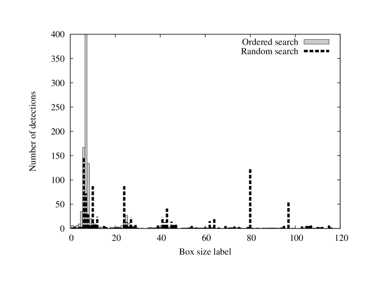
Figure 3.8: Number of detections as a function of box size when searching 1000 realisations of source “A” at 2Gpc. Results are shown when using the ordered search, and when the box size search order is randomized. The $x$-axis is the box size label, which corresponds to the order in which the boxes are analysed in the ordered search.

Given that we have specified thresholds so that each box size contributes equally to the overall false alarm probability we might expect the search to perform better if we restrict it to use only those few box sizes responsible for most of the detections of the injected signal. By eliminating box sizes that make few detections, we expect to reduce the overall false alarm probability while keeping the overall detection rate approximately constant, thereby improving the overall ROC performance.

This can be investigated by re-analysing the data using only a small subset (i.e., $20$) of the 119 box sizes originally considered, choosing the box sizes that were responsible for the most detections of EMRI source “A”. Having performed the search using only $20$ box sizes, we can eliminate the box size which has the worst performance (i.e., the least number of detections) in the $20$ box search and then repeat the search with the remaining $19$ box sizes. This process can be repeated, eliminating one box size each time, until only one box size remains. The box size that contributes the fewest detections depends to a limited extent on the (additional) false alarm probability assigned to each box size. We used the additional false alarm probability that gave an overall search false alarm probability of $\sim 10\%$ since, as argued earlier, this would be a reasonable value to use in the final LISA search.

The results of this targeting procedure are summarised in Table 3.1. When the number of box sizes is reduced from $119$ to $20$, the ROC performance does improve as the overall FAP reduces, while the detection rate remains largely unchanged. This improvement is of the order of $5\%$ in detection rate. As the number of box sizes used is reduced further, the ROC performance remains roughly constant until only $4$ box sizes are being used. Using fewer than $4$ box sizes leads to performance that degrades and is always worse than the full search. This is in keeping with the understanding that several box sizes are needed for efficient detection of a source due to the effect of noise fluctuations. We also computed results for the Excess Power search (full and targeted), and these are also summarised in the same Table. The trend as box sizes are removed is the same and HACR always outperforms the Excess Power search.

We conclude that it is possible to improve the performance of the search for a specific source by selecting fewer box sizes. However, the improvement is not hugely significant. This is consistent with what was found for the Excess Power search (Gair and Wen (2005) [70]). Since the box sizes that are efficient for the detection of one particular source will almost certainly not be the same as those that are efficient for other sources, the best approach is to include all the box sizes in the search. However, since there are certain box shapes that are good for detecting certain types of source, the box size for which a given detection is made provides a diagnostic of the source system. This will be discussed further in Sec. 3.10.3.

Table 3.1: Detection rates for various overall false alarm probabilities when using the HACR or Excess Power searches with a restricted number of box sizes.

Search	Detection rate at
	OFAP=$5\%$	OFAP=$10\%$	OFAP=$30\%$	OFAP=$60\%$
HACR, All bins	84.9%	89.3%	95.5%	98.7%
HACR, 20 bins	90.2%	92.9%	98.2%	99.7%
HACR, 10 bins	90.5%	93.4%	98.4%	99.6%
HACR, 7 bins	92.0%	94.7%	98.4%	99.4%
HACR, 4 bins	92.7%	95.0%	98.5%	99.4%
HACR, 1 bin	81.7%	87.5%	95.2%	99.0%
Excess Power, All bins	63.8%	71.5%	87.1%	95.4%
Excess Power, 10 bins	72.6%	81.4%	94.0%	98.2%
Excess Power, 7 bins	66.0%	76.0%	91.0%	98.1%
Excess Power, 4 bins	68.7%	78.5%	91.3%	98.4%
Excess Power, 1 bin	47.8%	59.1%	79.7%	93.8%

3.9.1 Detection of other EMRI sources

The results described in the preceding Sections have focused on the detection of one particular EMRI, source “A”. We have also explored the performance of HACR in detecting some of the other EMRI sources used for the investigation of the Excess Power search (Gair and Wen (2005) [70], see Table 1 for a summary). Specifically we used the sources “K” and “N”, which have the same parameters as source “A” except for eccentricity. The source “K” is initially circular, while source “N” has eccentricity of $0.7$, compared to $e=0.4$ for source “A”. We placed these sources at a range of distances between 1.8Gpc and 2.6Gpc, and injected them into noise realisations. We were thus able to determine ROC curves for detection of these sources via the method described in Sec. 3.8.1. In Fig. 3.9 we compare the ROC curves for detection of these sources with HACR when they are at a distance of 2Gpc. We see that our ability to detect a system at a given distance is better for binaries in circular orbits (source “K”) than for systems with eccentric orbits (sources “A” and “N”). This is consistent with what was found for the Excess Power search in Gair and Wen (2005) [70]. The predominant effect of orbital eccentricity is to split the gravitational wave radiation power into multiple harmonics. As the eccentricity increases, the frequencies of these harmonics become increasingly separated. As a consequence, a given box in the time-frequency map contains a smaller ratio of signal power to noise power. The detectability of EMRI sources therefore decreases as the eccentricity is increased.

The overall detectability of these new sources (“K” and “N”) with HACR follows the same pattern as the Excess Power search. HACR has a slightly greater detection rate than Excess Power when the source is nearby, but as the source is put further away, the performance of HACR and Excess Power become comparable before the random limit is reached. However, in all cases, the HACR detection is made with a smaller upper threshold ($\eta_{\rm{up}}^{n,l}$) than Excess Power, compensated by a larger pixel threshold ($N_{p}^{n,l}$). Thus, HACR detections identify clusters with significant numbers of pixels, the properties of which will be invaluable for subsequent parameter estimation. This will be discussed in Sec. 3.11.

Figure 3.9: ROC curves for detection of EMRI sources “A”, “K” and “N” at a distance of 2Gpc using HACR. These sources all have the same parameters except for their eccentricity.

3.9.2 Tuning HACR for multiple EMRI sources

In the preceding Sections, we have focused on detection of a single EMRI source at a fixed distance. However, in the actual analysis of LISA data, we will not know a priori what sources will be in the data stream, and so the HACR thresholds need to be tuned as generally as possible. Even in the case of a single EMRI source, the optimal threshold combination depends to some extent on the distance at which the source is placed. This is in contrast to the Excess Power search, where there is only one threshold that is uniquely determined by the choice of false alarm probability. There are two possible approaches to constructing a general HACR search: 1) have several separate HACR searches, targeting different sources and using different sets of thresholds or 2) have a single HACR search with a set of thresholds chosen to be sensitive to as many LISA sources as possible. We have focussed on the latter approach, since our results have shown that it is possible to do almost as well with a single set of “generic” thresholds as with source specific thresholds.

As a first step, we took the thresholds designed to optimally detect source “A” at 2Gpc and used those thresholds to search for sources “K” and “N”. We found that there was some degradation of performance, but that this was negligible. At an $OFAP$ of $10\%$, the detection rate for source “K” changed from $99.3\%$ to $99.7\%$, and that of source “N” changed from $18.4\%$ to $17.9\%$. This is a promising result and suggests that certain threshold combinations do well at detecting all the EMRI events. It is also possible to tune the thresholds to be generally sensitive to many different sources. This is not really necessary for the case of EMRI detection, but we will describe the procedure here as it will be needed when other types of sources are included in the search (this is discussed in Sec. 3.10).

We want to tune the search to maximize the total LISA event rate (i.e., the number of events observed). If we knew in advance which sources would be present in the LISA data, we could tune the search by considering multiple noise realisations with that family of sources injected and choosing the threshold combination that gives the maximum total detection rate for given $OFAP$. Since we do not know what the actual sources in the LISA data will be, we can instead tune the thresholds to be as sensitive as possible to a single event of unknown type, using prior knowledge to weight the relative likelihood of different types of events. This procedure ignores issues of source confusion, but should ensure that the loudest events are detected, no matter of what type or at what distance they might be.

In practice, tuning for multiple sources is done as follows:

• Generate realisations of noise with injected signals for each of the sources $s$ we want to include in the tuning.

• For the first box size, determine the rate of detections, $R_{s}({\bf t_{i}})$, of each of the signals when using HACR with each threshold triplet, ${\bf t_{i}}$, that yields a pre-chosen $AFAP$.

• Construct a sum over these rates for each threshold triplet, $\sum w_{s}R_{s}({\bf t_{i}})$, using an appropriate weighting factor, $w_{s}$, for each source.

• Choose the threshold triplet that maximizes this weighted sum. For each signal, identify the realisations in which that optimal threshold triplet gave a detection.

• Move onto the next box size, but for each signal search only realisations in which the optimal thresholds for the previous box size(s) did not yield any detections.

• Repeat for all box sizes.

One question is what to use for the weighting factors. If we knew that only one type of source existed in the Universe, but it was equally likely to be at any point in space, we want a volume weighted average. This is done by taking our set of sources to be a single given source placed at a sequence of distances, $d_{i}$. The source at distance $d_{i}$ can then be regarded to be representative of all sources in the range $d_{i-1}<d<d_{i}$, and should be weighted by the (Euclidean) volume of space in that range, $w_{i}\propto 4\pi(d_{i}^{3}-d_{i-1}^{3})/3$. We carried out this procedure using source “A” at distances of $1.8$Gpc, $2.0$Gpc, …, $2.6$Gpc, with weightings $1.8^{3}=5.832$, $2.0^{3}-1.8^{3}=2.168$, $2.2^{3}-2.0^{3}=2.648$ … $2.6^{3}-2.4^{3}=3.752$ (we have neglected common factors of $4\pi/3$). We took the closest source to be at $1.8$Gpc since up to that distance, the detection rate is always $100\%$. This appears to give artificial weight to the $1.8$Gpc source, but in practice this does not happen since virtually every threshold combination gives a $100\%$ detection rate for that source, and the variation in rate is determined primarily by the other injections. We used distance weighted thresholds to search for source “A” at various distances. The thresholds did change to some extent, but these changes were small since the optimal thresholds are almost independent of distance, and the overall ROC performance was largely unaffected. We deduce that it is possible to detect a given EMRI source at any distance with a single set of thresholds.

LISA will see more than one type of source, and we can fold in prior information about the relative abundance of different events by adjusting the weighting factors. We repeated the above, tuning for sources “A”, “K” and “N” at a single distance of $2$Gpc, and given equal weighting. In that case too, we found that the ROC performance was not significantly changed when tuning for these multiple sources. We also tuned for all three sources, placed at all the distances, $1.8$Gpc, …, $2.6$Gpc, with the volume weightings listed previously. Once again, the ROC performance was not significantly altered. Thus, there is a single set of HACR thresholds that can detect all three EMRI sources at any distance.

These results may not be truly generic, since the three EMRI sources are quite similar, differing only in eccentricity. It is therefore perhaps unsurprising that a single set of thresholds can detect all three sources almost optimally. However, we will see in Sec. 3.10.3 that this result carries over to the case when the sources have quite different characteristics. This is not totally surprising, since we know that HACR includes the Excess Power search as the pixel threshold $N_{p}=1$ limit. The Excess Power search thresholds are independent of the tuning source at fixed assigned FAP. Thus, a HACR search tuned for a collection of sources can do no worse than the Excess Power search for each of those sources. Since the HACR search does not seem to hugely outperform the Excess Power search, we would not anticipate that this combined tuning procedure would lead to a serious degradation of performance even when considering very different classes of sources.

3.10 Performance of HACR in detection of other LISA sources

We have shown that HACR may be successfully tuned in order to detect multiple EMRI sources with different parameters. In this Section we investigate HACR’s ability to detect other classes of signals, specifically white dwarf (WD) binaries and supermassive black hole (SMBH) binary mergers. We expect these other classes of signals to have quite different structures in a time-frequency map. A typical EMRI signal consists of several frequency components (due to the eccentricity of the orbit), which “chirp” slowly over the course of the observation, i.e., the frequency and amplitude increase. By contrast, the gravitational wave emission from a WD binary is essentially monochromatic. A SMBH binary inspiral also gives a chirping signal, but the chirp occurs much more quickly than the EMRI due to the increased mass ratio (see Eq. (3.5)), so it will be characterised by a signal that is broader in frequency. This difference in structure allows HACR to be tuned for all three types of source simultaneously.

3.10.1 A typical SMBH binary source

As a preliminary investigation, we repeated the tuning procedure described earlier, injecting a typical SMBH binary inspiral and a typical WD binary at various distances. The SMBH binary waveform represented the inspiral of two $10^{6}M_{\odot}$ non-spinning black holes, placed at a random sky position, and with merger occurring $\sim 3$ weeks before the end of the observation. As mentioned in Sec. 3.5, our SMBH injections use the waveform model given in Cutler (1998) [52]. This is a restricted post-Newtonian waveform accurate to 1.5PN. More accurate waveforms are available in the literature, with post-Newtonian corrections up to 3.5PN. However, the simple model captures the main features of a SMBH merger signal and is accurate enough for the more qualitative nature of this preliminary study. The quoted masses are the intrinsic masses of the black holes, i.e., not redshifted. When the source was placed at higher redshift there are two effects — an increase in the luminosity distance to the source, and a redshifting effect — which pushes the signal into the less sensitive part of the LISA noise curve.

In Figure 3.10 we show the ROC curves for detection of this SMBH binary source at a range of redshifts. At each redshift the optimal thresholds were chosen using the tuning method described in Section 3.8.1. We find that SMBH binary sources at redshifts $z\leq 3$ are detected with almost perfect efficiency using HACR, but we stop being able to resolve signals for redshifts $z>3.5$. This is primarily because the (matched-filtering, coherent) SNR of the source decreases significantly due to the redshifting effect mentioned above.

3.10.2 A typical white dwarf binary source

The “typical” white dwarf binary was chosen to have the parameters of RXJ0806.3+1527 (one of LISA’s “verification binaries” described in Stroeer and Vecchio (2006) [133]), except for distance and sky position. The latter was chosen randomly, but this choice, and the noise model used meant the SNR of this source at a distance of $1$kpc was approximately a factor of $3$ greater than that quoted in Stroeer and Vecchio (2006) [133]. This should be born in mind when considering the distances quoted in the following discussion. In Fig. 3.10 we show the ROC curve for this WD source, injected at various distances. At distances $\leq 15$kpc, we obtain near perfect detection using HACR. The sensitivity falls off rapidly for greater distances and the source becomes undetectable at greater than $\sim 20$kpc. Even allowing for the SNR discrepancy mentioned above, this source would be detectable at $\sim 6$–$7$kpc, i.e., almost at the distance of the galactic center. Since this particular source is estimated to be at a distance of $300$–$1000$pc, it would be detectable via this method. We would expect to detect other similar white dwarfs at distances of $1$–$10$kpc depending on the source parameters. This does not allow for source confusion, as we have only injected single sources into the data stream, but the conclusion for RXJ0806 should be robust, since it radiates at $\sim 6$mHz, which is in the regime where WD binaries are well separated in frequency (this can be seen in the results of population synthesis models described in Nelemans et al. (2001) [104] and is reflected in the LISA noise curve (Eq. (3.4.1)) in which the contribution from WD binaries, accounting for resolvability of sources, is below the instrumental noise at $6$mHz).

Figure 3.10: ROC curves for detection of a SMBH binary merger (upper panel) and a WD binary inspiral (lower panel) at various distances. The optimal thresholds for each distance were chosen using the tuning method described in Sec. 3.8.1

In the preceding plots, the HACR thresholds have been tuned to detect the source in question (either an EMRI or a WD binary or SMBH merger), at a particular distance. If instead we imagined that we would use only one set of thresholds, tuned for EMRI source “A” at a distance of 2Gpc, then the ROC performance for detection of the SMBH binary and WD binary events is significantly degraded. This is shown in Fig. 3.11, which compares the ROC curve for detection of the SMBH binary at a redshift of $z=3.125$ and the WD binary at a distance of $17$kpc when the EMRI thresholds are used, versus the result when the source specific tuned thresholds are used. We chose distances of $z=3.125$ and $17$kpc since in that case the sources are loud, but have less than a $100\%$ detection rate, so we will be able to see ROC variations. Figure 3.11 shows that using the EMRI thresholds to detect other sources typically reduces the detection rate by a factor of $\sim 5$ at an $OFAP$ of $10\%$.

Figure 3.11: ROC curves for detection of the SMBH and WD binary sources using thresholds tuned for EMRI source “A” at a distance of 2Gpc. For comparison, the ROC performance when the search is tuned for the source in question is also shown.

3.10.3 Tuning HACR for multiple classes of sources

One solution to this problem in a LISA search would be to run several independent searches focussed on different source families. However, it is also possible to tune a single set of HACR thresholds to be sensitive to all three types of sources simultaneously. This is done in the same way as the source and distance-averaged tuning described in Sec. 3.9.2, but now we inject not only EMRI signals, but also WD and SMBH signals. When the thresholds are tuned using EMRI source “A” at 2Gpc, the WD binary at 17kpc and the SMBH binary at $z=3.125$ with equal weighting, the detection rate at an $OFAP$ of $10\%$ for the EMRI source “A” at 2Gpc is $87.0\%$ as opposed to $89.3\%$ using optimal tuning.

This difference is of the same order as the expected error in our ROC estimates (see Sec. 3.8.1) and is therefore considered to be negligible. For the SMBH binary at $z=3.125$ and the WD binary at 17kpc the change in detection rate when using the thresholds tuned for all three sources when compared to the detection rate obtained using the optimal thresholds is also negligible. It is clear that when the thresholds are tuned for all three types of source, the performance of HACR is almost as high as the source specific searches, and still exceeds the performance of the Excess Power search.

This is due to the different time-frequency properties of the three types of sources. The time-frequency properties of a source determine which box sizes are good for its detection. This is illustrated in Fig. 3.12, which shows schematically all box sizes that contribute more than $1\%$ of the detection rate for four different sources: EMRIs “A” and “K”, the WD binary and the SMBH binary inspiral. Physically, we expect WD binary tracks to be virtually monochromatic, and of long duration. Therefore, we might expect to detect such sources in box sizes that are long in time but very narrow in frequency. The SMBH binary inspiral (at that redshift) is fairly short in duration, but sweeps through a reasonable range in frequency and is also quite loud. Therefore, we might expect to see it in boxes that are narrow in time, and broader in frequency.

EMRIs are similar in structure to SMBH binary inspirals, but last longer in time and evolve more slowly. For a circular EMRI (e.g., source “K”), one might expect to detect it in boxes that were long in time and quite narrow in frequency, although shorter in time and slightly broader in frequency than the WD binary (since the frequency changes as the source inspirals). However, an eccentric EMRI (e.g., source “A”) will have multiple frequency harmonics, and one might expect to do better using a slightly broader box in frequency which then includes more of the frequency components.

The distribution in Fig. 3.12 fits precisely with this physical intuition. When tuning for multiple sources, the threshold in a given box size will be determined by the source that the box size is most suited to detecting. The fact that the various types of sources favour distinct groups of box sizes means the overall performance is comparable to the source specific performance. The box sizes in which HACR detections are made thus provide an additional way to classify the source type.

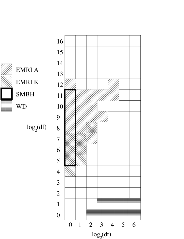
Figure 3.12: Box sizes in which the majority of detections are made for various sources. For each of four different sources — EMRI “A” at 2Gpc, EMRI “K” at 2Gpc, the SMBH binary at z=3.125 and the WD binary at 17kpc — we indicate all box sizes which were responsible for $>1\%$ of the detections of that source in 1000 realisations. The sources are identified by the patterns in the key. Box sizes that were good for several sources are indicated by multiple patterns, e.g. the box with co-ordinates (0,7).

3.11 Using HACR for parameter estimation

We have emphasised throughout this paper that, although the HACR search does not provide a much greater detection rate than the Excess Power search, the clusters it identifies may be used to characterise the source. Parameters estimated from HACR clusters can then be used as input for other algorithms in subsequent stages of a hierarchical search of the LISA data.

An Excess Power detection essentially contains only two pieces of information: the time and frequency at which the detection is made. Since we are using binning as part of the search, there is also some information contained in the box sizes used to bin the spectrograms in which the detections are made. To gain further information, a detection made by Excess Power must be followed by a track identification stage, and this is currently being investigated Wen et al. (2006) [147]. In contrast, a cluster identified by HACR consists not of one but many pixels. Thus, in addition to the previous properties, the HACR cluster has shape information which is potentially a much more powerful diagnostic. The information that we can extract includes the size of the event in time and frequency and the shape and curvature of the boundary of the cluster. An event that is short in the time direction but broad in frequency might be an instrumental noise burst, whereas events long in time and narrow in frequency are probably inspiral events.

The difference in frequency between the latest and earliest pixels in the cluster divided by the difference in time provides an estimate of the rate of change of frequency (or chirp rate) of the event. In Wen et al. (2006) [147] and Gair et al. (2007) [73] the authors show that by measuring the evolution of the frequency $f_{n}(t)$ and its derivative $\dot{f}_{n}(t)$ we can estimate six of the EMRI’s intrinsic parameters including both component masses, the spin of the SMBH, the orbital eccentricity and its inclination with respect to the spin of the SMBH as well as the system’s orbital frequency. The power profile along an inspiral track would reveal the modulations associated with the motion of the detector and thus provide a method to find the sources sky position (although it turns out that opposite points in the sky are degenerate). Figures 3.1 and 3.2 show spectrograms of our three EMRI signals. The amplitude modulation caused by LISA’s motion and the different harmonics caused by the orbit’s eccentricity can be seen.

Application of HACR for the Mock LISA Data Challenge

In Gair et al. (2007) [73] the authors used HACR to detect EMRI’s in simulated LISA data as part of the Mock LISA Data Challenge (MLDC, see Arnaud et al. (2006) [13] for an overview). In each of the five data sets provided (called $1.3.1$ - $1.3.5$) a single EMRI signal was embedded in simulated LISA noise (i.e., no confusion between different sources). HACR performed well and identified four of the five EMRI’s with clusters that enabled the authors to estimate the sources parameters to reasonable accuracy using the methods previously discussed. (see Table 1 of Gair et al. (2007) [73]). In the fifth case, an EMRI with relatively low SNR, only a small number of bright pixels were identified and parameter estimation was not performed.

Source confusion

As mentioned previously, source confusion is a major issue for LISA, with many events likely to be overlapping in time and frequency in the data stream. A detection in the time-frequency plane could therefore either be a single source or several overlapping sources. An analysis of the cluster boundary should be able to distinguish these two cases in certain situations, i.e., distinguish a “cross” from a “line”.

The shape parameters presented in Sahni et al. (1998) [126] may provide diagnostics which might be able to distinguish instrumental bursts from astrophysical bursts from long lived astrophysical events. A further use of a detected signal’s power profile would be to distinguish crossing tracks (clusters) caused by different inspiral events. In a more sophisticated analysis, cluster properties would allow different clusters that are generated by the same event to be identified. An EMRI is characterised by several different frequency components and these might well appear as different clusters in a time-frequency analysis (see spectrograms in Wen and Gair (2005) [148]). However, these tracks remain almost parallel as they evolve, and so the rate of change of frequency provides a way to connect the tracks in a second stage analysis of the HACR clusters. If tracks can be identified like this, the properties, such as the track separation, encode information about the orbital eccentricity etc.

One complication in all of this is that the construction of the binned spectrograms makes use of bins that overlap in time and frequency. This has the effect of smearing out tracks from astrophysical sources and noise events in the data, which complicates cluster characterisation and parameter extraction. In analysing cluster properties, this effect must be accounted for, or methods developed to deconvolve the effect of binning once a source has been identified.

It is clear that HACR cluster properties are a potentially powerful tool both for vetoing, i.e., distinguishing astrophysical events from instrumental artifacts, and for parameter estimation. Work is currently underway to investigate which of these and other cluster properties are most powerful as diagnostics, and how the system’s parameters may be estimated from them.

Chapter 4 Summary and Conclusions

From Einstein’s General Theory of Relativity we identify gravitational waves as perturbations to the curvature of spacetime caused by the acceleration of matter and which propagate at the speed of light. Gravitational waves cause a periodic strain (i.e., stretching and contraction) of the proper distance between points in spacetime as they pass and we describe how they can be detected using laser-interferometers.

Binary systems will lose energy and angular momentum through the emission of gravitational waves causing their orbits to shrink and leading to their eventual coalescence. In Chapter 2 we consider the challenging prospect of detecting gravitational waves from the orbital decay or inspiral of stellar mass binary systems with spinning components using the ground-based LIGO detectors. Using approximations to the Einstein equations we are able to produce predictions of the gravitational wave signals that would be observed from the inspiral of binaries consisting of compact objects, such as black holes and neutron stars. We employ matched-filtering, a method which requires accurate predictions of the gravitational wave signals we expect to observe, in order to identify gravitational wave signals in the noise-dominated detector data. The accurate predictions of the observed gravitational wave signal are our templates.

Interactions between the orbital angular momenta of the binary and the spin angular momenta of its components will cause the binaries orbital plane to precess which in turn leads to modulation of the amplitude and phase of the gravitational wave signal that will be observed. Matched-filter searches using templates which do not include the effects of spin may miss the gravitational wave signals emitted by binaries with spinning components.

Using post-Newtonian approximations to the Einstein equations we are able to produce templates for spin-modulated gravitational wave signals that are functions of the 17 physical parameters used to describe a binary system with spinning components. Unfortunately, using templates with this many parameters is very computationally expensive. Instead, we use a detection template family (DTF) which captures the essential features of the true gravitational wave signal but which is a function of fewer non-physical or phenomenological parameters. We use the post-Newtonian approximated waveforms as a target model used to assess the ability of our DTF to capture spin-modulated gravitational waves.

We describe the methods and results of the first dedicated search for gravitational waves emitted during the inspiral of compact binaries with spinning component bodies. Using the BCV2 DTF we performed a matched-filter search of $788$ hours of LIGO data collected during its third science run (S3). Details of the implementation of the detection template family and calculation of the signal to noise ratio are given in the Appendix. No detection of gravitational wave signals was made, but by estimating our search pipeline’s sensitivity to gravitational wave signals we are able to set a Bayesian upper limit on the rate of coalescence of stellar mass binaries. The upper limit on the rate of coalescence for prototypical NS-BH binaries with spinning component bodies was calculated to be $\mathcal{R}_{90\%}=15.9\,\mathrm{yr}^{-1}\,\mathrm{L_{10}}^{-1}$ once uncertainties had been marginalized over (see Sec. 2.8). The upper limits on the rate of coalescence we calculate are around 7 orders of magnitude larger than the rates predicted by population synthesis studies (see Sec. 2.1.1) and therefore do not allow us to constrain uncertainties in these studies.

Future searches for gravitational waves will benefit from improvements to the detectors used to collect the data as well as the algorithms we use to analyse it with. Data taken during LIGO’s fifth science run (S5) is greatly improved in both sensitivity and observation time (i.e., $\sim 1$ year of data with all three LIGO detectors simultaneously taking science quality data) than previous data sets. In 2007, during the final months of LIGO’s S5 run, the French-Italian detector Virgo began taking its first science quality data.

Preparation for a search of LIGO S5 data for binaries with spinning components utilising templates described by physical (rather than phenomenological) parameters [114, 39] is well underway. This new template family, which we shall call the PBCV family, has two significant advantages over the BCV2 DTF. In using physical parameters to describe the templates the PBCV family consists only of the physical waveforms predicted by our target model and does not allow for any non-physical waveforms that can arise using the BCV2 DTF. Therefore, in describing spin-modulated gravitational waves using fewer degrees of freedom than the BCV2 DTF, the PBCV family will have a lower false alarm rate and will consequently be able to use lower detection (SNR) thresholds. Also, since the PBCV templates are described using the physical parameters of the binary source they are better suited to parameter estimation than the BCV2 templates.

We found that the BCV2 DTF has good sensitivity to binary sources consisting of non-spinning, as well as spinning, components (see Fig. 2.13). However, compared to dedicated searches for systems with non-spinning components [5], the BCV2 DTF requires a larger number of templates (see Table II of Abbott et al. [5]) in order to capture the effects of spin and suffers from requiring a larger SNR threshold in order to reduce the number of triggers generated to a reasonable level. Instead, searches of LIGO S5 data for systems with non-spinning components are likely to use post-Newtonian waveforms which will benefit from using templates described by physical parameters (see discussion above regarding the PBCV family).

In Chapter 3 we turn our attention to developing data analysis algorithms for the planned space-based mission, LISA (Laser Interferometer Space Antenna). LISA will be sensitive to extreme mass ratio inspirals (EMRIs) during which a stellar mass compact object orbits and finally merges with a super massive black hole. An EMRI waveform will depend on up to 17 parameters (similarly to the stellar mass binaries we considered previously although in this case eccentricity cannot be neglected whereas the spin of the smaller body can be) and will be observable throughout the duration of LISA’s operation ($\sim 3$ years). Due to the long duration and complexity of the EMRI signals, matched-filter based searches will be extremely computationally expensive. We describe a less sensitive but computational cheap time-frequency based method that can be used to quickly identify the loudest few EMRI events.

The time-frequency method we describe combines and improves upon two previous algorithms. The Excess Power algorithm [148, 70] searches a time-frequency map (e.g., a spectrogram) for unusually bright pixels. This method works best when the power contained in the pixels of the time-frequency map are combined or binned so that a significant fraction of a gravitational wave signal’s power is contained within a single box. The Hierarchical Algorithm for Clusters and Ridges (HACR) [81] is somewhat more sophisticated and works by identifying an unusually bright pixel and then building around it a cluster of pixels whose power exceeds another (lower) threshold.

Our new algorithm, combines the binning stage of Excess Power with the cluster identification stage of HACR. We call our new algorithm HACR since it is simply an extension to the existing algorithm of the same name. The distance to which EMRI signals could be detected was similar for both HACR and for Excess Power. However, by associating a gravitational wave signal with a cluster of pixels rather than just one, we are able to extract more information about its source making HACR a potential first stage analysis in a hierarchical detection scheme. The estimation of parameters from time-frequency map events identified by HACR could be used to perform targeted (and therefore less computationally expensive) matched-filter based searches.

We are able to tune the thresholds involved in classifying a cluster of pixels as an event candidate in order to improve our sensitivity to particular EMRI source at a particular distance. We find that by setting different thresholds for the different boxes (created when we bin the power in the pixels of our time-frequency map) we are able to remain sensitive to a range of EMRI signals whilst also being able to detect white dwarf binaries (WDBs) and the merger of super massive black holes (SMBHs). This is possible because EMRIs, WDBs and SMBHs occupy different shaped regions of the time-frequency map and are therefore found by separate sets of boxes (see Fig. 3.12).

HACR was subsequently used to analyse data generated as part of the Mock LISA Data Challenge (MLDC) and identified four of the five EMRI signals [73]. Future developments to HACR should include both refinement of the estimation of the source’s parameters and methods to deal with the issue of source confusion, the overlapping of signals in the time-frequency plane discussed in Sec. 3.11.

Chapter 5 Appendix

5.1 Miscellaneous Derivations

5.1.1 Proof of Eq. (1.61)

We will prove that

$$\int T^{ij}d^{3}x=\frac{1}{2}\frac{d^{2}}{dt^{2}}\int x^{i}x^{j}T^{00}d^{3}x.$$ (5.1)

Using integration by parts:

$$\int_{a}^{b}u(x)\frac{dv(x)}{dx}dx=\left[u(x)v(x)\right]_{a}^{b}-\int_{a}^{b}v(x)\frac{du(x)}{dx}dx$$ (5.2)

we can write:

$$\int\frac{\partial}{\partial x^{k}}\underbrace{\frac{\partial T^{kl}}{\partial x^{l}}}_{v(x)}\underbrace{x^{i}x^{j}}_{u(x)}d^{3}x = \underbrace{\left[x^{i}x^{j}\frac{\partial T^{kl}}{\partial x^{l}}\right]}_{=0}-\int\frac{\partial T^{kl}}{\partial x^{l}}\frac{\partial}{\partial x^{k}}\left(x^{i}x^{j}\right)d^{3}x$$ (5.3)

$$= -\int\frac{\partial T^{kl}}{\partial x^{l}}\left(\delta^{kj}x^{i}+\delta^{ki}x^{j}\right)d^{3}x$$

where the integrand term in square brackets goes to zero since we evaluate the integral over a surface far from the source where $T^{kl}=0$. Integrating by parts again we can write:

$$-\int\frac{\partial}{\partial x^{l}}\underbrace{T^{kl}}_{v(x)}\underbrace{\left(\delta^{kj}x^{i}+\delta^{ki}x^{j}\right)}_{u(x)}d^{3}x = -\underbrace{\left[\left(\delta^{kj}x^{i}+\delta^{ki}x^{j}\right)T^{kl}\right]}_{=0}$$ (5.4)

$$+ \int T^{kl}\frac{\partial}{\partial x^{l}}\left(\delta^{kj}x^{i}+\delta^{ki}x^{j}\right)d^{3}x$$

$$= \int T^{kl}\left(\delta^{li}\delta^{kj}+\delta^{lj}\delta^{ki}\right)d^{3}x$$

$$= 2\int T^{ij}d^{3}x.$$

5.1.2 Response of Gaussian random variables to linear transformations

Consider a set of random variables $x$ where $\mbox{\boldmath$x$}^{T}=[x_{1},x_{2}\dots x_{N}]$ is a row vector of random variables. We will use matrix notation for convenience and have used a superscript $T$ to denote the transpose. We consider a set of random variables $x$ described by a multivariate Gaussian probability density function

$$p_{x}(\mbox{\boldmath$x$})=\frac{1}{(2\pi)^{N/2}|\mbox{\boldmath$C$}|^{1/2}}\mathrm{exp}\left[-\frac{1}{2}(\mbox{\boldmath$x$}-\mbox{\boldmath$\mu$})^{T}\mbox{\boldmath$C$}^{-1}(\mbox{\boldmath$x$}-\mbox{\boldmath$\mu$})\right]$$ (5.5)

where $\mu$ are the means of $x$, i.e., $\mbox{\boldmath$\mu$}^{T}=[\mu_{1},\mu_{2}\dots\mu_{N}]$. $C$ is the covariance matrix of the $x$ and $|\mbox{\boldmath$C$}|$ is the determinant of $C$. The covariance matrix $C$ of $x$ is defined as

$$C_{x}=\left(\begin{array}[]{cccc}\sigma^{2}_{1}&\dots&\rho_{1,N}\sigma_{1}\sigma_{N}\\ \vdots&\ddots&\vdots\\ \rho_{1,N}\sigma_{1}\sigma_{N}&\dots&\sigma^{2}_{N}\end{array}\right).$$ (5.9)

where $\sigma^{2}_{1}$ is the variance of $x_{1}$ and $\rho_{1,2}\sigma_{1}\sigma_{2}$ is the covariance between $x_{1}$ and $x_{2}$.

Finally, we will be interested in the linear transform of a multivariate Gaussian where each random variable $x_{i}$ is described by an (independent) Normal distribution with mean $\mu_{i}=0$ and variance $\sigma_{i}^{2}=1$.

We define a linear transform $L$ such that

$$\mbox{\boldmath$y$}=\mbox{\boldmath$L$}\mbox{\boldmath$x$}$$ (5.10)

and where its inverse is given by

$$\mbox{\boldmath$x$}=\mbox{\boldmath$\Gamma$}\mbox{\boldmath$y$}$$ (5.11)

where we have $\mbox{\boldmath$L$}\mbox{\boldmath$\Gamma$}=\mbox{\boldmath$I$}$ and $I$ is the identity matrix.

We will now find the probability density function $p_{y}$ of the output $x$ of the linear transformation Eq. (5.10). There will be a one-to-one mapping between the values of $x_{i}$ and $y_{i}$. Following [149] (Eqs. (1.12) to (1.14)) we find that

$$p_{y}(\mbox{\boldmath$y$})=|\mbox{\boldmath$J$}|p_{x}(\mbox{\boldmath$x$})$$ (5.12)

where $|\mbox{\boldmath$J$}|$ is the Jacobian determinant of the linear transformation $L$. The Jacobian of the transform $L$ from $x$ to $y$ is defined as

$$J_{xy}=\frac{\partial(x_{1},x_{2},\dots,x_{N})}{\partial(y_{1},y_{2},\dots,y_{N})}=\left(\begin{array}[]{ccc}\frac{\partial x_{1}}{\partial y_{1}}&\dots&\frac{\partial x_{N}}{\partial y_{1}}\\ \vdots&\ddots&\vdots\\ \frac{\partial x_{1}}{\partial y_{N}}&\dots&\frac{\partial x_{N}}{\partial y_{N}}\\ \end{array}\right).$$ (5.16)

The determinant of $J$ is simply the determinant of the reverse transformation, i.e., $|\mbox{\boldmath$J$}|=|\mbox{\boldmath$\Gamma$}|$. From the standard relation $|A|=1/|A^{-1}|$ we find that $|\mbox{\boldmath$J$}|=1/|\mbox{\boldmath$L$}|$.

Therefore we find the probability density function of $Y$ to be

$$p_{y}(\mbox{\boldmath$y$}) = |\mbox{\boldmath$J$}|p_{x}(\mbox{\boldmath$x$})$$ (5.17)

$$= \frac{1}{(2\pi)^{N/2}|\mbox{\boldmath$L$}|\cdot|\mbox{\boldmath$C$}|^{1/2}}\mathrm{exp}\left[-\frac{1}{2}\mbox{\boldmath$x$}^{T}\mbox{\boldmath$C$}^{-1}\mbox{\boldmath$x$}\right]$$ (5.18)

$$= \frac{1}{(2\pi)^{N/2}|\mbox{\boldmath$L$}||\mbox{\boldmath$C$}|^{1/2}}\mathrm{exp}\left[-\frac{1}{2}(\mbox{\boldmath$\Gamma$}\mbox{\boldmath$y$})^{T}\mbox{\boldmath$C$}^{-1}(\mbox{\boldmath$\Gamma$}\mbox{\boldmath$y$})\right]$$ (5.19)

where we have used $\mbox{\boldmath$x$}=\mbox{\boldmath$\Gamma$}\mbox{\boldmath$y$}$ to write the probability density function in terms of $y$. Following the derivation in [149] (Eqs. (4.26) to (4.28)) we define a new matrix $\mbox{\boldmath$F$}=\mbox{\boldmath$L$}\mbox{\boldmath$C$}\mbox{\boldmath$L$}^{T}$. Using this definition and standard matrix identities we can see that

$$(\mbox{\boldmath$\Gamma$}\mbox{\boldmath$y$})^{T}\mbox{\boldmath$C$}^{-1}(\mbox{\boldmath$\Gamma$}\mbox{\boldmath$y$}) = \mbox{\boldmath$y$}^{T}\mbox{\boldmath$\Gamma$}^{T}\mbox{\boldmath$C$}^{-1}\mbox{\boldmath$\Gamma$}\mbox{\boldmath$y$}$$ (5.20)

$$= \mbox{\boldmath$y$}^{T}(\mbox{\boldmath$L$}^{T})^{-1}\mbox{\boldmath$C$}^{-1}\mbox{\boldmath$L$}^{-1}\mbox{\boldmath$y$}$$ (5.21)

$$= \mbox{\boldmath$y$}^{T}(\mbox{\boldmath$L$}^{T}\mbox{\boldmath$C$}\mbox{\boldmath$L$})^{-1}\mbox{\boldmath$y$}$$ (5.22)

$$= \mbox{\boldmath$y$}^{T}\mbox{\boldmath$F$}^{-1}\mbox{\boldmath$y$}.$$ (5.23)

Using $|\mbox{\boldmath$A$}|^{T}=|\mbox{\boldmath$A$}|$ we can write the determinant $|\mbox{\boldmath$F$}|=|\mbox{\boldmath$L$}||\mbox{\boldmath$C$}||\mbox{\boldmath$L$}^{T}|=|\mbox{\boldmath$L$}|^{2}\cdot|\mbox{\boldmath$C$}|$. Rewriting $p_{y}(\mbox{\boldmath$y$})$ we find that it has the form of a multivariate Gaussian with covariance matrix $F$,

$$p_{Y}(\mbox{\boldmath$y$})=\frac{1}{(2\pi)^{N/2}|\mbox{\boldmath$F$}|^{1/2}}\mathrm{exp}\left[-\frac{1}{2}\mbox{\boldmath$y$}^{T}\mbox{\boldmath$F$}^{-1}\mbox{\boldmath$y$}\right].$$ (5.24)

We have therefore shown that the linear transformation (e.g., the matched-filtering) of a multivariate Gaussian distribution is also a multivariate Gaussian distribution.

5.2 Construction of orthonormalised amplitude functions

5.2.1 Definitions

The amplitude functions $\mathcal{A}_{k}(f_{\rm{cut}},\beta;f)$ to be orthonormalised are given below;

$$\mathcal{A}_{1}(f_{\rm{cut}},\beta;f) = f^{-7/6}\theta(f_{\rm{cut}}-f),$$

$$\mathcal{A}_{2}(f_{\rm{cut}},\beta;f) = f^{-7/6}\cos(\beta f^{-2/3})\theta(f_{\rm{cut}}-f),$$

$$\mathcal{A}_{3}(f_{\rm{cut}},\beta;f) = f^{-7/6}\sin(\beta f^{-2/3})\theta(f_{\rm{cut}}-f).$$ (5.25)

We shall denote the orthonormalised amplitude vectors as $\mathcal{\widehat{A}}_{k}(f_{\rm{cut}},\beta;f)$ and we shall use the Gram-Schmidt method to perform the orthonormalisation. The moments of the noise that will be used to abbreviate the expressions for the orthonormalised amplitude functions are given below;

$$I = 4\int_{f_{\rm{low}}}^{f_{\rm{cut}}}f^{-7/3}\frac{df}{S_{n}(f)},$$

$$J = 4\int_{f_{\rm{low}}}^{f_{\rm{cut}}}f^{-7/3}\cos(\beta f^{-2/3})\frac{df}{S_{n}(f)},$$

$$K = 4\int_{f_{\rm{low}}}^{f_{\rm{cut}}}f^{-7/3}\sin(\beta f^{-2/3})\frac{df}{S_{n}(f)},$$

$$L = 2\int_{f_{\rm{low}}}^{f_{\rm{cut}}}f^{-7/3}\sin(2\beta f^{-2/3})\frac{df}{S_{n}(f)},$$

$$M = 2\int_{f_{\rm{low}}}^{f_{\rm{cut}}}f^{-7/3}\cos(2\beta f^{-2/3})\frac{df}{S_{n}(f)},$$ (5.26)

where $S_{n}(f)$ is the one-sided noise power spectral density. Throughout these derivations we shall use $||a(f)||$ to represent the inner product of a function $a(f)$ with itself:

$$||a(f)||=\left<a(f),a(f)\right>$$ (5.27)

and we shall also abbreviate our equations by writing $\mathcal{A}_{k}(f_{\rm{cut}},\beta;f)$ as $\mathcal{A}_{k}$ (and similarly for the orthonormalised functions) with no change in meaning.

5.2.2 Finding $\mathcal{\widehat{A}}_{1}$

To perform the transformation from $\mathcal{A}_{1}$ to $\mathcal{\widehat{A}}_{1}$ we use

$$\mathcal{A}_{1}\to\mathcal{\widehat{A}}_{1}=\frac{\mathcal{A}_{1}}{||\mathcal{A}_{1}||^{1/2}}.$$ (5.28)

Finding $||\mathcal{A}_{1}||$;

$$||\mathcal{A}_{1}|| = \left<\mathcal{A}_{1},\mathcal{A}_{1}\right>$$ (5.29)

$$= 4\int_{f_{\rm{low}}}^{f_{\rm{cut}}}\mathcal{A}_{1}^{*}(f)\mathcal{A}_{1}(f)\frac{df}{S_{n}(f)}.$$

Substituting in for $\mathcal{A}_{1}$, multiplying terms together and rewriting integrals in terms of moments of the noise;

$$||\mathcal{A}_{1}||=4\int_{f_{\rm{low}}}^{f_{\rm{cut}}}f^{-7/3}\frac{df}{S_{n}(f)}=I.$$ (5.30)

Substituting back into Eq. (5.28) for $\mathcal{\widehat{A}}_{1}$;

$$\mathcal{\widehat{A}}_{1}=\frac{f^{-7/6}}{I^{1/2}}.$$ (5.31)

5.2.3 Finding $\mathcal{\widehat{A}}_{2}$

To perform the transformation from $\mathcal{A}_{2}$ to $\mathcal{\widehat{A}}_{2}$ we use;

$$\mathcal{A}_{2}\to\mathcal{\widehat{A}}_{2} = \frac{\mathcal{A}_{2}-\left<\mathcal{A}_{2},\mathcal{\widehat{A}}_{1}\right>\mathcal{\widehat{A}}_{1}}{||\mathcal{A}_{2}-\left<\mathcal{A}_{2},\mathcal{\widehat{A}}_{1}\right>\mathcal{\widehat{A}}_{1}||^{1/2}}.$$ (5.32)

Finding $\left<\mathcal{A}_{2},\mathcal{\widehat{A}}_{1}\right>$;

$$\left<\mathcal{A}_{2},\mathcal{\widehat{A}}_{1}\right>=4\int_{f_{\rm{low}}}^{f_{\rm{cut}}}\mathcal{A}_{2}^{*}(f)\mathcal{\widehat{A}}_{1}(f)\frac{df}{S_{n}(f)}.$$ (5.33)

Substituting in for $\mathcal{A}_{2}$ and $\mathcal{\widehat{A}}_{1}$, multiplying terms together and rewriting integrals in terms of moments of the noise;

$$\left<\mathcal{A}_{2},\mathcal{\widehat{A}}_{1}\right> = \frac{4}{I^{1/2}}\int_{f_{\rm{low}}}^{f_{\rm{cut}}}f^{-7/3}\cos(\beta f^{-2/3})\frac{df}{S_{n}(f)}$$ (5.34)

$$= \frac{J}{I^{1/2}}.$$

Finding numerator of $\mathcal{\widehat{A}}_{2}$, $\mathcal{A}_{2}-\left<\mathcal{A}_{2},\mathcal{\widehat{A}}_{1}\right>\mathcal{\widehat{A}}_{1}$;

$$\mathcal{A}_{2}-\left<\mathcal{A}_{2},\mathcal{\widehat{A}}_{1}\right>\mathcal{\widehat{A}}_{1}=f^{-7/6}\cos(\beta f^{-2/3})-\frac{J}{I}f^{-7/6}.$$ (5.35)

Finding $||\mathcal{A}_{2}-\left<\mathcal{A}_{2},\mathcal{\widehat{A}}_{1}\right>\mathcal{\widehat{A}}_{1}||$;

$$||\mathcal{A}_{2}-\left<\mathcal{A}_{2},\mathcal{\widehat{A}}_{1}\right>\mathcal{\widehat{A}}_{1}|| = \left<\mathcal{A}_{2}-\left<\mathcal{A}_{2},\mathcal{\widehat{A}}_{1}\right>\mathcal{\widehat{A}}_{1},\mathcal{A}_{2}-\left<\mathcal{A}_{2},\mathcal{\widehat{A}}_{1}\right>\mathcal{\widehat{A}}_{1}\right>$$ (5.36)

$$= 4\int_{f_{\rm{low}}}^{f_{\rm{cut}}}(\mathcal{A}_{2}-\left<\mathcal{A}_{2},\mathcal{\widehat{A}}_{1}\right>\mathcal{\widehat{A}}_{1})^{2}\frac{df}{S_{n}(f)}.$$

Finding $(\mathcal{A}_{2}-\left<\mathcal{A}_{2},\mathcal{\widehat{A}}_{1}\right>\mathcal{\widehat{A}}_{1})^{2}$;

$$(\mathcal{A}_{2}-\left<\mathcal{A}_{2},\mathcal{\widehat{A}}_{1}\right>\mathcal{\widehat{A}}_{1})^{2} = \bigg{[}f^{-7/6}\cos(\beta f^{-2/3})-f^{-7/6}\frac{J}{I}\bigg{]}^{2}$$ (5.37)

$$= f^{-7/3}\cos^{2}(\beta f^{-2/3})+\frac{J^{2}}{I^{2}}f^{-7/3}$$

$$- 2\frac{J}{I}f^{-7/3}\cos(\beta f^{-2/3}).$$

Substituting into Eq. (5.36) for $||\mathcal{A}_{2}-\left<\mathcal{A}_{2},\mathcal{\widehat{A}}_{1}\right>\mathcal{\widehat{A}}_{1}||$;

$$||\mathcal{A}_{2} - \left<\mathcal{A}_{2},\mathcal{\widehat{A}}_{1}\right>\mathcal{\widehat{A}}_{1}||$$ (5.38)

$$= 4\int_{f_{\rm{low}}}^{f_{\rm{cut}}}\bigg{[}f^{-7/3}\cos^{2}(\beta f^{-2/3})+\frac{J^{2}}{I^{2}}f^{-7/3}-2\frac{J}{I}f^{-7/3}\cos(\beta f^{-2/3})\bigg{]}\frac{df}{S_{n}(f)}$$

$$= 4\int_{f_{\rm{low}}}^{f_{\rm{cut}}}f^{-7/3}\cos^{2}(\beta f^{-2/3})\frac{df}{S_{n}(f)}+4\frac{J^{2}}{I^{2}}\int_{f_{\rm{low}}}^{f_{\rm{cut}}}f^{-7/3}\frac{df}{S_{n}(f)}$$

$$- 8\frac{J}{I}\int_{f_{\rm{low}}}^{f_{\rm{cut}}}f^{-7/3}\cos(\beta f^{-2/3})\frac{df}{S_{n}(f)}.$$

Using $\cos^{2}(\beta f^{-2/3})=\frac{1}{2}[1+\cos(2\beta f^{-2/3})]$ and rewriting integrals in terms of moments of the noise;

$$||\mathcal{A}_{2}-\left<\mathcal{A}_{2},\mathcal{\widehat{A}}_{1}\right>\mathcal{\widehat{A}}_{1}||=M+\frac{I}{2}-\frac{J^{2}}{I}.$$ (5.39)

Substituting back into Eq. (5.30) for $\mathcal{\widehat{A}}_{2}$;

$$\mathcal{\widehat{A}}_{2}=\frac{f^{-7/6}\cos(\beta f^{-2/3})-\frac{J}{I}f^{-7/6}}{\bigg{[}M+\frac{I}{2}-\frac{J^{2}}{I}\bigg{]}^{1/2}}$$ (5.40)

and simplifying;

$$\mathcal{\widehat{A}}_{2}=\frac{f^{-7/6}\bigg{[}\cos(\beta f^{-2/3})-\frac{J}{I}\bigg{]}I^{1/2}}{\bigg{[}IM+\frac{I^{2}}{2}-J^{2}\bigg{]}^{1/2}}.$$ (5.41)

5.2.4 Finding $\mathcal{\widehat{A}}_{3}$

To perform the transformation from $\mathcal{A}_{3}$ to $\mathcal{\widehat{A}}_{3}$ we use;

$$\mathcal{A}_{3}\to\mathcal{\widehat{A}}_{3}=\frac{\mathcal{A}_{3}-\left<\mathcal{A}_{3},\mathcal{\widehat{A}}_{1}\right>\mathcal{\widehat{A}}_{1}-\left<\mathcal{A}_{3},\mathcal{\widehat{A}}_{2}\right>\mathcal{\widehat{A}}_{2}}{||\mathcal{A}_{3}-\left<\mathcal{A}_{3},\mathcal{\widehat{A}}_{1}\right>\mathcal{\widehat{A}}_{1}-\left<\mathcal{A}_{3},\mathcal{\widehat{A}}_{2}\right>\mathcal{\widehat{A}}_{2}||}.$$ (5.42)

Finding $\left<\mathcal{A}_{3},\mathcal{\widehat{A}}_{1}\right>$;

$$\left<\mathcal{A}_{3},\mathcal{\widehat{A}}_{1}\right>=4\int_{f_{\rm{low}}}^{f_{\rm{cut}}}\mathcal{A}_{3}^{*}(f)\mathcal{\widehat{A}}_{1}(f)\frac{df}{S_{n}(f)}$$ (5.43)

Substituting in for $\mathcal{A}_{3}$ and $\mathcal{\widehat{A}}_{1}$, multiplying terms together and rewriting integrals in terms of moments of the noise;

$$\left<\mathcal{A}_{3},\mathcal{\widehat{A}}_{1}\right> = \frac{4}{I^{1/2}}\int_{f_{\rm{low}}}^{f_{\rm{cut}}}f^{-7/3}\sin(\beta f^{-2/3})\frac{df}{S_{n}(f)}$$ (5.44)

$$= \frac{K}{I^{1/2}}.$$ (5.45)

Finding $\left<\mathcal{A}_{3},\mathcal{\widehat{A}}_{2}\right>$;

$$\left<\mathcal{A}_{3},\mathcal{\widehat{A}}_{2}\right>=4\int_{f_{\rm{low}}}^{f_{\rm{cut}}}\mathcal{A}_{3}^{*}(f)\mathcal{\widehat{A}}_{2}(f)\frac{df}{S_{n}(f)}.$$ (5.46)

Substituting in for $\mathcal{A}_{3}$ and $\mathcal{\widehat{A}}_{2}$ and multiplying terms together;

$$\left<\mathcal{A}_{3},\mathcal{\widehat{A}}_{2}\right> = \frac{I^{1/2}}{\bigg{[}IM+\frac{I^{2}}{2}-J^{2}\bigg{]}^{1/2}}$$ (5.47)

$$\times \left[4\int_{f_{\rm{low}}}^{f_{\rm{cut}}}f^{-7/3}\sin(\beta f^{-2/3})\cos(\beta f^{-2/3})\frac{df}{S_{n}(f)}\right.$$

$$- \left.\frac{4J}{I}\int_{f_{\rm{low}}}^{f_{\rm{cut}}}f^{-7/3}\sin(\beta f^{-2/3})\frac{df}{S_{n}(f)}\right].$$ (5.48)

Using $2\sin(\beta f^{-2/3})\cos(\beta f^{-2/3})=\sin(2\beta f^{-2/3})$;

$$\left<\mathcal{A}_{3},\mathcal{\widehat{A}}_{2}\right> = \frac{I^{1/2}}{\bigg{[}IM+\frac{I^{2}}{2}-J^{2}\bigg{]}^{1/2}}$$ (5.49)

$$\times \left[2\int_{f_{\rm{low}}}^{f_{\rm{cut}}}f^{-7/3}\sin(2\beta f^{-2/3})\frac{df}{S_{n}(f)}\right.$$

$$- \left.\frac{4J}{I}\int_{f_{\rm{low}}}^{f_{\rm{cut}}}f^{-7/3}\sin(\beta f^{-2/3})\frac{df}{S_{n}(f)}\right].$$

Rewriting in terms of moments of the noise;

$$\left<\mathcal{A}_{3},\mathcal{\widehat{A}}_{2}\right> = \frac{I^{1/2}}{\bigg{[}IM+\frac{I^{2}}{2}-J^{2}\bigg{]}^{1/2}}\bigg{[}L-\frac{JK}{I}\bigg{]}$$ (5.50)

$$= \frac{IL-JK}{I^{1/2}\bigg{[}IM+\frac{I^{2}}{2}-J^{2}\bigg{]}^{1/2}}.$$

Finding numerator of $\mathcal{\widehat{A}}_{3}$, $\mathcal{A}_{3}-\left<\mathcal{A}_{3},\mathcal{\widehat{A}}_{1}\right>\mathcal{\widehat{A}}_{1}-\left<\mathcal{A}_{3},\mathcal{\widehat{A}}_{2}\right>\mathcal{\widehat{A}}_{2}$;

$$\mathcal{A}_{3}-\left<\mathcal{A}_{3},\mathcal{\widehat{A}}_{1}\right>\mathcal{\widehat{A}}_{1}-\left<\mathcal{A}_{3},\mathcal{\widehat{A}}_{2}\right>\mathcal{\widehat{A}}_{2}=f^{-7/6}$$ (5.51)

$$\times \left[\sin(\beta f^{-2/3})-\frac{K}{I}-\frac{IL-JK}{\bigg{[}IM+\frac{I^{2}}{2}-J^{2}\bigg{]}}\left[\cos(\beta f^{-2/3})-\frac{J}{I}\right]\right].$$

Finding $||\mathcal{A}_{3}-\left<\mathcal{A}_{3},\mathcal{\widehat{A}}_{1}\right>\mathcal{\widehat{A}}_{1}-\left<\mathcal{A}_{3},\mathcal{\widehat{A}}_{2}\right>\mathcal{\widehat{A}}_{2}||$;

$$||\mathcal{A}_{3} - \left<\mathcal{A}_{3},\mathcal{\widehat{A}}_{1}\right>\mathcal{\widehat{A}}_{1}-\left<\mathcal{A}_{3},\mathcal{\widehat{A}}_{2}\right>\mathcal{\widehat{A}}_{2}||$$ (5.52)

$$= 4\int_{f_{\rm{low}}}^{f_{\rm{cut}}}\left[\mathcal{A}_{3}-\left<\mathcal{A}_{3},\mathcal{\widehat{A}}_{1}\right>\mathcal{\widehat{A}}_{1}-\left<\mathcal{A}_{3},\mathcal{\widehat{A}}_{2}\right>\mathcal{\widehat{A}}_{2}\right]^{2}\frac{df}{S_{n}(f)}.$$

Finding $\left[\mathcal{A}_{3}-\left<\mathcal{A}_{3},\mathcal{\widehat{A}}_{1}\right>\mathcal{\widehat{A}}_{1}-\left<\mathcal{A}_{3},\mathcal{\widehat{A}}_{2}\right>\mathcal{\widehat{A}}_{2}\right]^{2}$;

$$\left[\mathcal{A}_{3}\right. - \left.\left<\mathcal{A}_{3},\mathcal{\widehat{A}}_{1}\right>\mathcal{\widehat{A}}_{1}-\left<\mathcal{A}_{3},\mathcal{\widehat{A}}_{2}\right>\mathcal{\widehat{A}}_{2}\right]^{2}$$ (5.53)

$$= f^{-7/3}\Bigg{[}\sin^{2}(\beta f^{-2/3})+\frac{K^{2}}{I^{2}}$$

$$+ \frac{(IL-JK)^{2}}{\bigg{[}IM+\frac{I^{2}}{2}-J^{2}\bigg{]}^{2}}\bigg{[}\cos^{2}(\beta f^{-2/3})-\frac{2J}{I}\cos(\beta f^{-2/3})+\frac{J^{2}}{I^{2}}\bigg{]}$$

$$- \frac{2K}{I}\sin(\beta f^{-2/3})+\frac{2(IL-JK)}{IM+\frac{I^{2}}{2}-J^{2}}\bigg{[}\frac{K}{I}\sin(\beta f^{-2/3})-\frac{JK}{I}$$

$$- \sin(\beta f^{-2/3})\cos(\beta f^{-2/3})+\frac{J}{I}\sin(\beta f^{-2/3})\bigg{]}\Bigg{]}.$$

Using double angle formulas to simplify the equation;

$$(\mathcal{A}_{3} - \left<\mathcal{A}_{3},\mathcal{\widehat{A}}_{1}\right>\mathcal{\widehat{A}}_{1}-\left<\mathcal{A}_{3},\mathcal{\widehat{A}}_{2}\right>\mathcal{\widehat{A}}_{2})^{2}$$ (5.54)

$$= f^{-7/3}\Bigg{[}\frac{1}{2}-\frac{1}{2}\cos(2\beta f^{-2/3})+\frac{K^{2}}{I^{2}}$$

$$+ \frac{(IL-JK)^{2}}{\bigg{[}IM+\frac{I^{2}}{2}-J^{2}\bigg{]}^{2}}\bigg{[}\frac{1}{2}+\frac{1}{2}\cos(2\beta f^{-2/3})-\frac{2J}{I}\cos(\beta f^{-2/3})+\frac{J^{2}}{I^{2}}\bigg{]}$$

$$- \frac{2K}{I}\sin(\beta f^{-2/3})+\frac{2(IL-JK)}{IM+\frac{I^{2}}{2}-J^{2}}\bigg{[}\frac{K}{I}\cos(\beta f^{-2/3})-\frac{JK}{I^{2}}$$

$$- \frac{1}{2}\sin(2\beta f^{-2/3})+\frac{J}{I}\sin(\beta f^{-2/3})\bigg{]}\Bigg{]}.$$

Substituting into Eq. (5.52) for $||\mathcal{A}_{3}-\left<\mathcal{A}_{3},\mathcal{\widehat{A}}_{1}\right>\mathcal{\widehat{A}}_{1}-\left<\mathcal{A}_{3},\mathcal{\widehat{A}}_{2}\right>\mathcal{\widehat{A}}_{2}||$;

$$||\mathcal{A}_{3} - \left<\mathcal{A}_{3},\mathcal{\widehat{A}}_{1}\right>\mathcal{\widehat{A}}_{1}-\left<\mathcal{A}_{3},\mathcal{\widehat{A}}_{2}\right>\mathcal{\widehat{A}}_{2}||$$ (5.55)

$$= 2\int_{f_{\rm{low}}}^{f_{\rm{cut}}}f^{-7/3}\frac{df}{S_{n}(f)}-2\int_{f_{\rm{low}}}^{f_{\rm{cut}}}f^{-7/3}\cos(2\beta f^{-2/3})\frac{df}{S_{n}(f)}$$

$$+ \frac{4K^{2}}{I^{2}}\int_{f_{\rm{low}}}^{f_{\rm{cut}}}f^{-7/3}\frac{df}{S_{n}(f)}$$

$$+ \frac{(IL-JK)^{2}}{\bigg{[}IM+\frac{I^{2}}{2}-J^{2}\bigg{]}^{2}}\bigg{[}2\int_{f_{\rm{low}}}^{f_{\rm{cut}}}f^{-7/3}\frac{df}{S_{n}(f)}$$

$$+ 2\int_{f_{\rm{low}}}^{f_{\rm{cut}}}f^{-7/3}\cos(2\beta f^{-2/3})\frac{df}{S_{n}(f)}$$

$$- \frac{8J}{I}\cos(\beta f^{-2/3})\frac{df}{S_{n}(f)}+\frac{4J^{2}}{I^{2}}\int_{f_{\rm{low}}}^{f_{\rm{cut}}}f^{-7/3}\frac{df}{S_{n}(f)}\bigg{]}$$

$$- \frac{8K}{I}\int_{f_{\rm{low}}}^{f_{\rm{cut}}}f^{-7/3}\sin(\beta f^{-2/3})\frac{df}{S_{n}(f)}$$

$$+ \frac{(IL-JK)}{IM+\frac{I^{2}}{2}-J^{2}}\bigg{[}\frac{8K}{I}\int_{f_{\rm{low}}}^{f_{\rm{cut}}}f^{-7/3}\cos(\beta f^{-2/3})\frac{df}{S_{n}(f)}$$

$$- \frac{8JK}{I^{2}}\int_{f_{\rm{low}}}^{f_{\rm{cut}}}f^{-7/3}\frac{df}{S_{n}(f)}-4\int_{f_{\rm{low}}}^{f_{\rm{cut}}}f^{-7/3}\sin(2\beta f^{-2/3})\frac{df}{S_{n}(f)}$$

$$+ \frac{8J}{I}\int_{f_{\rm{low}}}^{f_{\rm{cut}}}f^{-7/3}\sin(\beta f^{-2/3})\frac{df}{S_{n}(f)}\bigg{]}.$$

Rewriting integrals in terms of moments of the noise;

$$||\mathcal{A}_{3} - \left<\mathcal{A}_{3},\mathcal{\widehat{A}}_{1}\right>\mathcal{\widehat{A}}_{1}-\left<\mathcal{A}_{3},\mathcal{\widehat{A}}_{2}\right>\mathcal{\widehat{A}}_{2}||$$ (5.56)

$$= \frac{1}{I}\bigg{[}\frac{I^{2}}{2}-IM-K^{2}-\frac{(IL-JK)^{2}}{IM+\frac{I^{2}}{2}-J^{2}}\bigg{]}$$

Substituting in Eq. (5.51) and Eq. (5.56) into Eq. (5.42) for $\mathcal{\widehat{A}}_{3}$;

$$\mathcal{\widehat{A}}_{3} = \frac{f^{-7/6}\Bigg{[}\sin(\beta f^{-2/3})-\frac{K}{I}-\frac{IL-JK}{IM+\frac{I^{2}}{2}-J^{2}}\bigg{[}\cos(\beta f^{-2/3})-\frac{J}{I}\bigg{]}\Bigg{]}I^{1/2}}{\bigg{[}\frac{I^{2}}{2}-IM-K^{2}-\frac{(IL-JK)^{2}}{IM+\frac{I^{2}}{2}-J^{2}}\bigg{]}^{1/2}}.$$

5.3 Documentation of the BCVSpin matched-filter engine

5.3.1 Introduction

This document describes the functions that have been written to perform matched-filtering of time-domain interferometric detector data using the detection templates developed by Buonanno, Chen and Vallisneri in BCV2 [40]. These functions have been written in C within the LSC Algorithm Library (Sec. 5.3.1) and can be found in lal/packages/findchirp/src in the following files:

Function	Filename
LALFindChirpBCVSpinTemplate()	FindChirpBCVSpinTemplate.c
LALFindChirpBCVSpinFilterSegment()	FindChirpBCVSpinFilter.c

These functions draw heavily upon pre-existing LAL functionality.

LSC Algorithm Library

The LSC Algorithm Library (LAL) is a software package which has been developed by the LIGO Laboratory (LL) and the LIGO Scientific Collaboration for the purpose of analysing data from interferometric gravitational wave detectors. To enable as many contributors as possible LAL is written in C which was thought to be the language the majority of contributors would be most proficient in. A full specification of LAL as well as downloadable versions of the code and documentation is available at the LAL Home Page [1]. Functions written in LAL (e.g., calibration of detector data, estimation of power spectral density, calculation of template bank metric, matched-filtering) are organised to perform higher level tasks (e.g., creating a template bank and measuring of triggers) using the LALapps (LAL Applications) package. LAL is freely available and distributed under the GNU General Public License. The FindChirp package, included within LAL, which performs the matched-filter routines used for inspiral searches is described in Allen et al. (2005) [7].

5.3.2 Definitions

Consider a time series $h(t)$ sampled at $N$ (numPoints) consecutive points with sampling interval $\Delta t$ (deltaT), that is;

$$h_{j}\equiv h(t_{j})\qquad t_{j}=j\Delta t$$ (5.58)

where the sampling frequency $f_{s}$ is given by

$$f_{s}=\frac{1}{\Delta t}$$ (5.59)

and the sampling interval $\Delta f$ is given by

$$\Delta f=\frac{1}{N\Delta t}.$$ (5.60)

Discrete Fourier Transforms

The forward DFT used by LAL is

$$\tilde{h}_{k}=\sum_{j=0}^{N-1}h_{j}e^{-2\pi ijk/N}$$ (5.61)

where $i=\sqrt{-1}$. We can recover the frequency series using

$$\tilde{h}(f_{k})=\Delta t\tilde{h_{k}}.$$ (5.62)

The reverse DFT used by LAL is

$$h(t_{j})=\frac{1}{N}\sum_{k=0}^{N-1}\tilde{h}_{k}e^{2\pi ijk/N}.$$ (5.63)

In practise we use the Fast Fourier Transform to perform (forward and reverse) DFTs. A DFT would typically require $\sim N^{2}$ arithmetic (floating point) operations. Using Fast Fourier Transforms (FFTs) (see e.g., Chapter 12 of Ref. [120] for a description) these transformations can be performed in only $\sim N\log N$ operations.

Discrete inner product

In practice the factor $1/N$ is omitted by the function performing the reverse DFT. The inner product of two time series $x(t_{j})$ and $y(t_{j})$ is defined as

$$\left<x(t_{j}),y(t_{j})\right>=4\Delta f\Re\sum_{k=0}^{N/2}\frac{\tilde{x}(f_{k})^{*}\tilde{y}(f_{k})}{S_{n}(f_{k})}$$ (5.64)

which is equivalent to

$$\left<x(t_{j}),y(t_{j})\right>=\frac{4\Delta t}{N}\Re\sum_{k=0}^{N/2}\frac{\tilde{x}_{k}^{*}\tilde{y}_{k}}{S_{n}(f_{k})}$$ (5.65)

where $S_{n}(f_{k})$ is the one-sided noise power spectral density defined as

$$\overline{\tilde{n}(f_{k})\tilde{n}^{*}(f^{\prime}_{k})}=\frac{1}{2}S_{n}(f_{k})\delta(f_{k}-f^{\prime}_{k})$$ (5.66)

and a superscript $*$ above a quantity indicates that its complex conjugate has been taken. We will define a normalised template (or waveform) $\hat{h}$ such that $\left<\hat{h},\hat{h}\right>=1$. To normalise a template $h$ we say that $\hat{h}=Ah$. Therefore

$$\left<\hat{h},\hat{h}\right>=\frac{4A^{2}\Delta t}{N}\Re\sum_{k=0}^{N/2}\frac{\tilde{h}_{k}^{*}\tilde{h}_{k}}{S_{n}(f_{k})}=1$$ (5.67)

It follows that

$$A=\left[\frac{4\Delta t}{N}\Re\sum_{k=0}^{N/2}\frac{\tilde{h}_{k}^{*}\tilde{h}_{k}}{S_{n}(f_{k})}\right]^{-1/2}$$ (5.68)

BCVSpin detection templates

Here we define a set of orthonormal templates ${\hat{h}}$ (in the frequency domain)

$$\hat{h}=\sum_{l=1}^{2n}\hat{\alpha}_{l}\hat{h}_{l}\qquad n=3$$ (5.69)

where

$$\hat{h}_{l}(t_{j};f_{k}) = \widehat{\mathcal{A}}_{l}(f_{k})e^{i\psi_{\rm{NM}}(f_{k})}e^{ijk/N}$$

$$\hat{h}_{l+n}(t_{j};f_{k}) = i\widehat{\mathcal{A}}_{l}(f_{k})e^{i\psi_{\rm{NM}}(f_{k})}e^{ijk/N}$$ (5.70)

where $l=1,2,3$, $n=3$ and $\hat{\alpha}_{l}$ are values corresponding to the amplitudes of each basis template (vector) $\hat{h}_{l}$. The vectors $\widehat{\mathcal{A}}_{l}$ are called the orthonormalised amplitude vectors and are given later by Eq. (5.81). To ensure that the templates are normalised,

$$\left<\hat{h},\hat{h}\right>=1$$ (5.71)

then it must be true that

$$\sum_{l=1}^{2n}\hat{\alpha}_{l}^{2}=1\qquad n=3$$ (5.72)

Using the relation $f_{k}=k\Delta f=k/(N\Delta t)$ we can find the discretized form of the various powers of frequency we use in the construction of the detection templates

$$f_{k}^{q}=\left(\frac{k}{N\Delta t}\right)^{q}\qquad k=1\dots\frac{N}{2}.$$ (5.73)

In practise we store arrays containing $(k/N)^{q}$ and then include the factor $\Delta t^{-q}$ as required .

5.3.3 BCVSpin matched-filter engine

Calibrating the strain data

Take FFT of time series data $x(t_{j})$

$$\tilde{x_{k}}=\sum_{j=0}^{N-1}x_{j}e^{-2\pi ijk/N}$$ (5.74)

Calculate the strain $\tilde{s_{k}}$

$$\tilde{s_{k}}=\tilde{x_{k}}\times R_{k}\qquad k=0\dots\frac{N}{2}$$ (5.75)

where

$$R_{k}={\tt response}_{k}\times{\tt dynRange}$$ (5.76)

where response is a complex vector ($k=0\dots N/2$) and dynRange is a single user defined value used to artificially adjust the magnitude of the strain. This is useful since realistic strains caused by gravitational wave events will be of the order $\sim 10^{-22}$ and it is easier to deal with quantities with values of around unity. Henceforth we shall refer to the strain $s$ as the detector output.

Calculation of inverse noise power spectrum

Calculating the inverse noise power spectrum $\tilde{\omega}_{v}(f_{k})$

$$\tilde{\omega}_{v}(f_{k})=\left\{\begin{array}[]{cl}0&k=0\dots k_{\rm{min}}-1\\ \frac{1}{S_{n}(f_{k})}&k=k_{\rm{min}}\dots N/2\end{array}\right.$$

where

$$k_{\rm{min}}=\frac{f_{\rm{low}}}{\Delta f}$$ (5.77)

Converting $\tilde{\omega}_{v}(k)$ to $\tilde{\omega}_{h}(k)$

$$\tilde{\omega}_{h}(f_{k})=\frac{\tilde{\omega}_{v}(f_{k})}{R_{k}R^{*}_{k}}$$ (5.78)

LALFindChirpBCVSpinTemplate()

We calculate the non-modulational phase of template as

$$\psi_{\rm{NM}}(f_{k})=\left\{\begin{array}[]{cl}0&k=0\dots k_{\rm{min}}-1\\ f_{k}^{-5/3}(\psi_{0}+f_{k}\psi_{3})&k=k_{\rm{min}}\dots k_{\rm{max}}-1\\ 0&k=k_{\rm{max}}\dots N/2\end{array}\right.$$

where

$$k_{\rm{min}}=\frac{f_{\rm{low}}}{\Delta f}\qquad k_{\rm{max}}=\frac{f_{\rm{cut}}}{\Delta f}.$$ (5.79)

$f_{\rm{low}}$ is the detectors lower frequency cutoff (see Sec. 2.6.3) and $f_{\rm{cut}}$ will eventually be supplied by the template bank.

We now calculate the moments of the noise required to construct the orthonormalised amplitude functions $\widehat{\mathcal{A}}_{l}$

$$I = 4\Delta f\,\sum_{k_{\rm{min}}}^{k_{\rm{max}}}f_{k}^{-7/3}\tilde{\omega}_{h}(f_{k})$$

$$J = 4\Delta f\,\sum_{k_{\rm{min}}}^{k_{\rm{max}}}f_{k}^{-7/3}\cos(\beta f^{-2/3})\tilde{\omega}_{h}(f_{k})$$

$$K = 4\Delta f\,\sum_{k_{\rm{min}}}^{k_{\rm{max}}}f_{k}^{-7/3}\sin(\beta f^{-2/3})\tilde{\omega}_{h}(f_{k})$$

$$L = 2\Delta f\,\sum_{k_{\rm{min}}}^{k_{\rm{max}}}f_{k}^{-7/3}\sin(2\beta f^{-2/3})\tilde{\omega}_{h}(f_{k})$$

$$M = 2\Delta f\,\sum_{k_{\rm{min}}}^{k_{\rm{max}}}f_{k}^{-7/3}\cos(2\beta f^{-2/3})\tilde{\omega}_{h}(f_{k})$$

and

$$\left.\begin{array}[]{c}I\\ J\\ K\\ L\\ M\end{array}\right\}=\left\{\begin{array}[]{cl}0&k=0\dots k_{\rm{min}}-1\\ 0&k=k_{\rm{max}}\dots N/2.\end{array}\right.$$

In practise we use omit prefactors of $\Delta t^{7/3}$ when calculating these moments. We can construct the orthonormalised amplitude functions, in the range $k_{\rm{min}}\geq k<k_{\rm{max}}$

$$\mathcal{\widehat{A}}_{1}(f_{k}) = f_{k}^{-7/6}\frac{1}{I^{1/2}}$$ (5.81)

$$\mathcal{\widehat{A}}_{2}(f_{k}) = f_{k}^{-7/6}\frac{\bigg{[}\cos(\beta f^{-2/3})-\frac{J}{I}\bigg{]}I^{1/2}}{\bigg{[}IM+\frac{I^{2}}{2}-J^{2}\bigg{]}^{1/2}}$$

$$\mathcal{\widehat{A}}_{3}(f_{k}) = f_{k}^{-7/6}\frac{\bigg{[}\sin(\beta f^{-2/3})-\frac{K}{I}-\frac{IL-JK}{IM+\frac{I^{2}}{2}-J^{2}}\big{[}\cos(\beta f^{-2/3})-\frac{J}{I}\big{]}\bigg{]}I^{1/2}}{\bigg{[}\frac{I^{2}}{2}-IM-K^{2}-\frac{(IL-JK)^{2}}{IM+\frac{I^{2}}{2}-J^{2}}\bigg{]}^{1/2}}$$

and

$$\left.\begin{array}[]{c}\mathcal{\widehat{A}}_{1}(f_{k})\\ \mathcal{\widehat{A}}_{2}(f_{k})\\ \mathcal{\widehat{A}}_{3}(f_{k})\end{array}\right\}=\left\{\begin{array}[]{cl}0&k=0\dots k_{\rm{min}}-1\\ 0&k=k_{\rm{max}}\dots N/2.\end{array}\right.$$

In practise we use omit factors of $\Delta t^{7/6}$ from the $f_{k}^{-7/6}$ prefactor terms in these functions. We find that the factors of $\Delta t$ in these terms and in the calculation of the noise moments cancel meaning that our amplitude functions are correctly scaled.

We can calculate the cross products of the orthonormalised amplitude functions

$$\left<\widehat{\mathcal{A}}_{l}(f_{k}),\widehat{\mathcal{A}}_{m}(f_{k})\right>=4\Delta f\,\sum_{k=0}^{N/2}\widehat{\mathcal{A}}_{l}(f_{k})\widehat{\mathcal{A}}_{m}(f_{k})\tilde{\omega}_{h}(f_{k})\qquad l,m=1,2,3$$ (5.82)

These results can be used to check that the amplitude functions are truly orthonormal

$$\left<\widehat{\mathcal{A}}_{l}(f_{k}),\widehat{\mathcal{A}}_{m}(f_{k})\right>=\delta_{l,m}$$ (5.83)

where

$$\delta_{l,m}=\left\{\begin{array}[]{cl}1&l=m\\ 0&l\neq m.\end{array}\right.$$

LALFindChirpBCVSpinFilterSegment()

We calculate the quantities $\tilde{q}_{n}(k)$ and use these to calculate the overlaps between the detector output $s$ and the orthonormalised basis templates $\hat{h}_{j}$

$$\tilde{q}_{l}(k)=\widehat{\mathcal{A}}_{l}(f_{k})e^{i\psi_{\rm{NM}}}\tilde{s}^{*}_{k}\tilde{\omega}_{h}(f_{k})$$ (5.84)

where $l=1,2,3$. The overlaps between the detector output $s$ and the 6 basis templates $\hat{h}_{l}$ can then be found at every time $t_{j}$:

$$\left<s,\hat{h}_{l}(t_{j})\right> = \frac{4}{N}\Re\sum_{k=0}^{N-1}\tilde{q}_{l}(k)e^{2\pi ijk/N}$$ (5.85)

$$\left<s,\hat{h}_{l+n}(t_{j})\right> = -\frac{4}{N}\Im\sum_{k=0}^{N-1}\tilde{q}_{l}(k)e^{2\pi ijk/N}$$ (5.86)

where $l=1,2,3$ and $n=3$. The factor of $1/N$ arises from the need to include a factor $\Delta t$ to convert from $\tilde{s}_{k}$ and $\tilde{s}(f_{k})$. Multiplying the existing factor of $\Delta f$ used in the definition of the inner product (see Eq. (5.64)) and the factor $\Delta t$ gives $1/N$. Using the overlaps calculated above we can find the signal to noise ratio $\rho$ of the detector output $s$ with the normalised template $\hat{h}$ at every time $t_{j}$:

$$\rho(t_{j})=\sqrt{\sum_{l=1}^{6}\left<s,\tilde{h}_{l}(t_{j})\right>^{2}}.$$ (5.87)

We note that we can calculate $\rho(t)$ for all the times we filter using the (Fast) Fourier transform (see Sec. 2.4.1). We can now find the individual $\hat{\alpha}_{l}$ values which correspond to the maxima in $\rho$, $\rho_{\rm{max}}$:

$$\hat{\alpha}_{l}=\frac{\left<s,\tilde{h}_{l}\right>_{\rm{max}}}{\rho_{\rm{max}}}\qquad l=1,2\dots 6.$$ (5.88)

We can then use these values to reconstruct the (normalised) waveform which caused the peak in $\rho$ using Eq. (5.69). The reconstruction of waveforms can be used to test the code when performing injections of known waveforms.

References

- [1] LSC Algorithm Library software packages: lal, lalapps, pylal and glue. http://www.lsc-group.phys.uwm.edu/lal.
- [2] B. Abbott et al. Analysis of LIGO data for gravitational waves from binary neutron stars. Phys. Rev. D, 69:122001, 2004.
- [3] B. Abbott et al. Search for gravitational waves from galactic and extra-galactic binary neutron stars. Phys. Rev. D, 72:082001, 2005.
- [4] B. Abbott et al. Search for gravitational waves from binary black hole inspirals in LIGO data. Phys. Rev. D, 73:062001, 2006.
- [5] B. Abbott et al. Search for gravitational waves from binary inspirals in S3 and S4 LIGO data. Physical Review D (Particles, Fields, Gravitation, and Cosmology), 77(6):062002, 2008.
- [6] Alex Abramovici et al. LIGO: The Laser Interferometer Gravitational wave Observatory. Science, 256:325, 1992.
- [7] Bruce Allen, Warren G. Anderson, Patrick R. Brady, Duncan A. Brown, and Jolien D. E. Creighton. Findchirp: An algorithm for detection of gravitational waves from inspiraling compact binaries. http://www.citebase.org/abstract?id=oai:arXiv.org:gr-qc/0509116, 2005.
- [8] Pau Amaro-Seoane, Jonathan R. Gair, Marc Freitag, M. Coleman Miller, Ilya Mandel, Curt J. Cutler, and Stanislav Babak. Astrophysics, detection and science applications of intermediate- and extreme mass-ratio inspirals. http://www.citebase.org/abstract?id=oai:arXiv.org:astro-ph/0703495, 2007.
- [9] Warren G. Anderson and Jolien D. E. Creighton. Searches for gravitational waves from binary neutron stars: A review. http://www.citebase.org/abstract?id=oai:arXiv.org:0712.2523, 2007.
- [10] T. A. Apostolatos. Search templates for gravitational waves from precessing, inspiraling binaries. Physical Review D (Particles, Fields, Gravitation, and Cosmology), 52:605, 1995.
- [11] Theocharis A. Apostolatos. Construction of a template family for the detection of gravitational waves from coalescing binaries. Phys. Rev. D, 54(4):2421–2437, Aug 1996.
- [12] Theocharis A. Apostolatos, Curt Cutler, Gerald J. Sussman, and Kip S. Thorne. Spin-induced orbital precession and its modulation of the gravitational waveforms from merging binaries. Phys. Rev. D, 49(12):6274–6297, Jun 1994.
- [13] K. A. Arnaud, S. Babak, J. G. Baker, M. J. Benacquista, N. J. Cornish, C. Cutler, S. L. Larson, B. S. Sathyaprakash, M. Vallisneri, A. Vecchio, and J.-Y. Vinet. The Mock LISA Data Challenges: An overview. http://www.citebase.org/abstract?id=oai:arXiv.org:gr-qc/0609105, 2006.
- [14] K. G. Arun, Bala R. Iyer, B. S. Sathyaprakash, and Pranesh A. Sundararajan. Erratum: Parameter estimation of inspiralling compact binaries using 3.5 post-Newtonian gravitational wave phasing: The nonspinning case [phys. rev. d 71, 084008 (2005)]. Physical Review D (Particles, Fields, Gravitation, and Cosmology), 72(6):069903, 2005.
- [15] K. G. Arun, Bala R Iyer, B. S. Sathyaprakash, and Pranesh A Sundararajan. Parameter estimation of inspiralling compact binaries using 3.5 post-Newtonian gravitational wave phasing: The nonspinning case. Physical Review D (Particles, Fields, Gravitation, and Cosmology), 71(8):084008, 2005.
- [16] P. Astone, D. Babusci, L. Baggio, M. Bassan, D. G. Blair, M. Bonaldi, P. Bonifazi, D. Busby, P. Carelli, M. Cerdonio, E. Coccia, L. Conti, C. Cosmelli, S. D’Antonio, V. Fafone, P. Falferi, P. Fortini, S. Frasca, G. Giordano, W. O. Hamilton, I. S. Heng, E. N. Ivanov, W. W. Johnson, A. Marini, E. Mauceli, M. P. McHugh, and R. Mezzena. Methods and results of the IGEC search for burst gravitational waves in the years 1997 - 2000. Phys. Rev. D, 68(2):022001, Jul 2003.
- [17] S. Babak, R. Balasubramanian, D. Churches, T. Cokelaer, and B. S. Sathyaprakash. A template bank to search for gravitational waves from inspiralling compact binaries I: Physical models. Classical and Quantum Gravity, 23:5477, 2006.
- [18] Stanislav Babak, Hua Fang, Jonathan R. Gair, Kostas Glampedakis, and Scott A. Hughes. “Kludge” gravitational waveforms for a test-body orbiting a kerr black hole. Physical Review D, 75:024005, 2007.
- [19] R. Balasubramanian, B. S. Sathyaprakash, and S. V. Dhurandhar. Gravitational waves from coalescing binaries: Detection strategies and Monte Carlo estimation of parameters. Phys. Rev. D, 53(6):3033–3055, Mar 1996.
- [20] Leor Barack and Curt Cutler. LISA capture sources: Approximate waveforms, signal-to-noise ratios, and parameter estimation accuracy. Physical Review D (Particles, Fields, Gravitation, and Cosmology), 69(8):082005, 2004.
- [21] R. M. Barnett, C. D. Carone, D. E. Groom, T. G. Trippe, C. G. Wohl, B. Armstrong, P. S. Gee, G. S. Wagman, F. James, M. Mangano, K. Mönig, L. Montanet, J. L. Feng, H. Murayama, J. J. Hernández, A. Manohar, M. Aguilar-Benitez, C. Caso, R. L. Crawford, M. Roos, N. A. Törnqvist, K. G. Hayes, K. Hagiwara, K. Nakamura, M. Tanabashi, K. Olive, and K. Honscheid. Review of particle physics. Phys. Rev. D, 54(1):1–708, Jul 1996.
- [22] Krzysztof Belczynski, Vassiliki Kalogera, and Tomasz Bulik. A comprehensive study of binary compact objects as gravitational wave sources: Evolutionary channels, rates, and physical properties. The Astrophysical Journal, 572:407, 2002.
- [23] Rahul Biswas, Patrick R. Brady, Jolien D. E. Creighton, and Stephen Fairhurst. The loudest event statistic: General formulation, properties and applications. http://www.citebase.org/abstract?id=oai:arXiv.org:0710.0465, 2007.
- [24] Luc Blanchet. Energy losses by gravitational radiation in inspiraling compact binaries to 5/2 post-Newtonian order. Phys. Rev. D, 54(2):1417–1438, Jul 1996.
- [25] Luc Blanchet. Innermost circular orbit of binary black holes at the third post-Newtonian approximation. Phys. Rev. D, 65(12):124009, May 2002.
- [26] Luc Blanchet. Erratum: Energy losses by gravitational radiation in inspiraling compact binaries to 5/2 post-Newtonian order [phys. rev. d 54, 001417 (1996)]. Physical Review D (Particles, Fields, Gravitation, and Cosmology), 71(12):129904, 2005.
- [27] Luc Blanchet, Thibault Damour, Gilles Esposito-Farese, and Bala R. Iyer. Gravitational radiation from inspiralling compact binaries completed at the third post-Newtonian order. Physical Review Letters, 93(9):091101, 2004.
- [28] Luc Blanchet, Thibault Damour, and Bala R. Iyer. Gravitational waves from inspiralling compact binaries: Energy loss and waveform to second-post-Newtonian order. Phys. Rev. D, 51(10):5360–5386, May 1995.
- [29] Luc Blanchet, Thibault Damour, Bala R. Iyer, Clifford M. Will, and Alan G. Wiseman. Gravitational-radiation damping of compact binary systems to second post-Newtonian order. Phys. Rev. Lett., 74(18):3515–3518, May 1995.
- [30] Luc Blanchet, Guillaume Faye, Bala R. Iyer, and Benoit Joguet. Gravitational-wave inspiral of compact binary systems to 7/2 post-Newtonian order. Phys. Rev. D, 65(6):061501, Feb 2002.
- [31] Luc Blanchet, Bala R. Iyer, and Benoit Joguet. Gravitational waves from inspiraling compact binaries: Energy flux to third post-Newtonian order. Phys. Rev. D, 65(6):064005, Feb 2002.
- [32] Luc Blanchet, Bala R. Iyer, and Benoit Joguet. Erratum: Gravitational waves from inspiraling compact binaries: Energy flux to third post-Newtonian order [phys. rev. 65, 064005 (2002)]. Physical Review D (Particles, Fields, Gravitation, and Cosmology), 71(12):129903, 2005.
- [33] P. R. Brady, J. D. E. Creighton, and A. G. Wiseman. Upper limits on gravitational-wave signals based on loudest events. Class. Quant. Grav., 21:S1775–S1781, 2004.
- [34] Laura W. Brenneman and Christopher S. Reynolds. Constraining black hole spin via X-ray spectroscopy. The Astrophysical Journal, 652:1028, 2006.
- [35] Chris Van Den Broeck and Anand S. Sengupta. Phenomenology of amplitude-corrected post-Newtonian gravitational waveforms for compact binary inspiral. I. Signal-to-noise ratios. Classical and Quantum Gravity, 24:155, 2007.
- [36] Robert G. Brown. Webpage deriving Green’s function for the wave equation. http://www.phy.duke.edu/rgb/Class/phy319/phy319/node56.html.
- [37] Alessandra Buonanno, Yanbei Chen, Yi Pan, Hideyuki Tagoshi, and Michele Vallisneri. Detecting gravitational waves from precessing binaries of spinning compact objects. II. Search implementation for low-mass binaries. Physical Review D (Particles, Fields, Gravitation, and Cosmology), 72(8):084027, 2005.
- [38] Alessandra Buonanno, Yanbei Chen, Yi Pan, Hideyuki Tagoshi, and Michele Vallisneri. Detecting gravitational waves from precessing binaries of spinning compact objects. II. Search implementation for low-mass binaries. Phys. Rev. D, 72:084027, 2005.
- [39] Alessandra Buonanno, Yanbei Chen, Yi Pan, and Michele Vallisneri. Quasiphysical family of gravity-wave templates for precessing binaries of spinning compact objects: Application to double-spin precessing binaries. Physical Review D (Particles, Fields, Gravitation, and Cosmology), 70(10):104003, 2004.
- [40] Alessandra Buonanno, Yanbei Chen, and Michele Vallisneri. Detecting gravitational waves from precessing binaries of spinning compact objects: Adiabatic limit. Phys. Rev. D, 67(10):104025, May 2003.
- [41] Alessandra Buonanno, Yanbei Chen, and Michele Vallisneri. Detection template families for gravitational waves from the final stages of binary black-hole inspirals: Nonspinning case. Phys. Rev. D, 67(2):024016, Jan 2003.
- [42] M. Burgay, N. D’Amico, A. Possenti, R. N. Manchester, A. G. Lyne, B. C. Joshi, M. A. McLaughlin, M. Kramer, J. M. Sarkissian, F. Camilo, V. Kalogera, C. Kim, and D. R. Lorimer. An increased estimate of the merger rate of double neutron stars from observations of a highly relativistic system. Nature, 426(6966):531–533, 2003.
- [43] Manuela Campanelli, Carlos O. Lousto, Yosef Zlochower, and David Merritt. Large merger recoils and spin flips from generic black-hole binaries. The Astrophysical Journal, 659:L5, 2007.
- [44] S. Chatterji. The search for gravitational-wave transients in data from the second LIGO science run. MIT Ph.D. Thesis, 2005.
- [45] N. Christensen et al. Veto studies LIGO inspiral triggers. Class. Quant. Grav., 22:S1059–S1068, 2005.
- [46] The LIGO Scientific Collaboration. Search of S3 LIGO data for gravitational wave signals from spinning black hole and neutron star binary inspirals. http://www.citebase.org/abstract?id=oai:arXiv.org:0712.2050, 2007, approved for publication in Phys. Rev. D.
- [47] Committee on NASA’s Beyond Einstein Program: An Architecture for Implementation Space Studies Board and Board on Physics and Astronomy Division on Engineering and Physical Sciences. NASA’s Beyond Einstein Program: An Architecture for Implementation. http://books.nap.edu/openbook.php?record_id=12006&page=R1, 2007.
- [48] Gregory B. Cook, Stuart L. Shapiro, and Saul A. Teukolsky. Rapidly rotating neutron stars in general relativity: Realistic equations of state. Astrophys. J., 424:823, 1994.
- [49] Neil J. Cornish and Jeff Crowder. LISA data analysis using markov chain monte carlo methods. Physical Review D (Particles, Fields, Gravitation, and Cosmology), 72(4):043005, 2005.
- [50] Neil J. Cornish and Edward K. Porter. Catching super massive black hole binaries without a net. Physical Review D, 75:021301, 2007.
- [51] Elena Cuoco, Giovanni Losurdo, Giovanni Calamai, Leonardo Fabbroni, Massimo Mazzoni, Ruggero Stanga, Gianluca Guidi, and Flavio Vetrano. Noise parametric identification and whitening for LIGO 40-meter interferometer data. Physical Review D, 64:122002, 2001.
- [52] Curt Cutler. Angular resolution of the LISA gravitational wave detector. Phys. Rev. D, 57(12):7089–7102, Jun 1998.
- [53] Thibault Damour, Bala R. Iyer, and B. S. Sathyaprakash. Comparison of search templates for gravitational waves from binary inspiral. Phys. Rev. D, 63(4):044023, Jan 2001.
- [54] Thibault Damour, Bala R. Iyer, and B. S. Sathyaprakash. Comparison of search templates for gravitational waves from binary inspiral: 3.5PN update. Phys. Rev. D, 66(2):027502, Jul 2002.
- [55] Shane W. Davis, Chris Done, and Omer M. Blaes. Testing accretion disk theory in black hole X-ray binaries. The Astrophysical Journal, 647:525, 2006.
- [56] Ray d’Inverno. Introducing Einstein’s Relativity. Clarendon Press, Oxford, Faculty of Mathematical Studies, University of Southampton.
- [57] R. Schödel et al. A star in a 15.2-year orbit around the supermassive black hole at the centre of the milky way. Nature (Letters), 419:694–696, 2002.
- [58] B. Abbott et al. for the LIGO Scientific Collaboration and ALLEGRO Collaboration. First cross-correlation analysis of interferometric and resonant-bar gravitational-wave data for stochastic backgrounds. Physical Review D (Particles, Fields, Gravitation, and Cosmology), 76(2):022001, 2007.
- [59] L. Baggio et al. for the LIGO Scientific Collaboration and AURIGA Collaboration. A joint search for gravitational wave bursts with AURIGA and LIGO. Classical and Quantum Gravity, 25(9):095004 (16pp), 2008.
- [60] Danzmann K et al. of the LISA study team. LISA - Laser Interferometer Space Antenna, Pre-Phase A Report. Max-Planck-Institut für Quantenoptic Report MPQ 233, 1998.
- [61] Stephen Fairhurst and Patrick Brady. Interpreting the results of searches for gravitational waves from coalescing binaries. http://www.citebase.org/abstract?id=oai:arXiv.org:0707.2410, 2007.
- [62] Lee S. Finn. Detection, measurement, and gravitational radiation. Phys. Rev. D, 46(12):5236–5249, Dec 1992.
- [63] Lee Samuel Finn and David F. Chernoff. Observing binary inspiral in gravitational radiation: One interferometer. Phys. Rev. D, 47(6):2198–2219, Mar 1993.
- [64] First Lock of the 2 Kilometer Interferometer at LIGO Hanford Observatory. http://www.ligo.caltech.edu/LIGO_web/firstlock/.
- [65] Daniel Sigg (for the LIGO Scientific Collaboration). Status of the LIGO detectors. Classical and Quantum Gravity, 25(11):114041 (8pp), 2008.
- [66] Michael Landry (for the LIGO Scientific Collaboration). Improvements in strain calibration for the third ligo science run. Classical and Quantum Gravity, 22(18):S985–S994, 2005.
- [67] V. Quetsche (for the LIGO Scientific Collaboration). LIGO - coherent optical length measurement with m accuracy. Proceedings of the 14th Coherent Laser Radar Conference.
- [68] J. M. Fregeau, S. L. Larson, M. C. Miller, R. O’Shaughnessy, and F. A. Rasio. Observing IMBH-IMBH Binary Coalescences via Gravitational Radiation. Astrophysical journal, 646:L135–L138, August 2006.
- [69] Marc Freitag. Monte carlo cluster simulations to determine the rate of compact star inspiralling to a central galactic black hole. Classical and Quantum Gravity, 18(19):4033–4038, 2001.
- [70] Jonathan Gair and Linqing Wen. Detecting extreme mass ratio inspirals with LISA using time-frequency methods ii: search characterization. Classical and Quantum Gravity, 22:S1359, 2005.
- [71] Jonathan R. Gair, Leor Barack, Teviet Creighton, Curt Cutler, Shane L. Larson, E. Sterl Phinney, and Michele Vallisneri. Event rate estimates for LISA extreme mass ratio capture sources. Classical and Quantum Gravity, 21:S1595, 2004.
- [72] Jonathan R Gair and Kostas Glampedakis. Improved approximate inspirals of test bodies into kerr black holes. Physical Review D (Particles, Fields, Gravitation, and Cosmology), 73(6):064037, 2006.
- [73] Jonathan R. Gair, Ilya Mandel, and Linqing Wen. Time-frequency analysis of extreme-mass-ratio inspiral signals in mock LISA data. http://www.citebase.org/abstract?id=oai:arXiv.org:0710.5250, 2007.
- [74] Gabriela Gonzalez. Limiting noises in gravitational wave detectors: guidance from their statistical properties, 2003.
- [75] Philippe Grandclément, Mia Ihm, Vassiliki Kalogera, and Krzysztof Belczynski. Searching for gravitational waves from the inspiral of precessing binary systems: Astrophysical expectations and detection efficiency of “spiky” templates. Physical Review D (Particles, Fields, Gravitation, and Cosmology), 69(10):102002, 2004.
- [76] Philippe Grandclément, Vassiliki Kalogera, and Alberto Vecchio. Searching for gravitational waves from the inspiral of precessing binary systems: Problems with current waveforms. Phys. Rev. D, 67(4):042003, Feb 2003.
- [77] Jenny E. Greene and Luis C. Ho. The mass function of active black holes in the local Universe. http://www.citebase.org/abstract?id=oai:arXiv.org:0705.0020, 2007.
- [78] Rémi Hakim. An Introduction to Relativistic Gravitation. Cambridge University Press, Département d’Astrophysique Relativiste et de Cosmologie, Observatoire de Meudon (France), 1999.
- [79] E. T. Harlaftis and J. Greiner. The rotational broadening and the mass of the donor star of GRS 1915+105. ASTRON.ASTROPHYS., 414:L13, 2004.
- [80] James B. Hartle. Gravity, an introduction to Einstein’s General Relativity. Addison Wesley, University of California, Santa Barbara, 2003.
- [81] I S Heng, R Balasubramanian, B S Sathyaprakash, and B F Schutz. First steps towards characterizing the Hierarchical Algorithm for Curves and Ridges pipeline. Classical and Quantum Gravity, 21(5):S821–S826, 2004.
- [82] R. M. Hjellming and M. P. Rupen. Episodic ejection of relativistic jets by the X-ray transient GRO J1655 - 40. Nature, 375:464–468, 1995.
- [83] R. A. Hulse and J. H. Taylor. Discovery of a pulsar in a binary system. Astrophysical Journal, 195:L51–L53, January 1975.
- [84] A. H. Jaffe and D. C. Backer. Gravitational waves probe the coalescence rate of massive black hole binaries. The Astrophysical Journal, 583(2):616–631, 2003.
- [85] Jonathan R. Gair and Gareth Jones. Detecting extreme mass ratio inspiral events in LISA data using the Hierarchical Algorithm for Clusters and Ridges (HACR). Classical and Quantum Gravity, 24:1145, 2007.
- [86] Jonathan R. Gair and Gareth Jones. Detecting LISA sources using time-frequency techniques. http://www.citebase.org/abstract?id=oai:arXiv.org:gr-qc/0703040, 2007.
- [87] V. Kalogera. Spin-orbit misalignment in close binaries with two compact objects. The Astrophysical Journal, 541:042003, 2000.
- [88] V. Kalogera, K. Belczynski, C. Kim, R. O’Shaughnessy, and B. Willems. Formation of double compact objects. http://www.citebase.org/abstract?id=oai:arXiv.org:astro-ph/0612144, 2006.
- [89] V. Kalogera, C. Kim, D. R. Lorimer, M. Burgay, N. D’Amico, A. Possenti, R. N. Manchester, A. G. Lyne, B. C. Joshi, M. A. McLaughlin, M. Kramer, J. M. Sarkissian, and F. Camilo. The cosmic coalescence rates for double neutron star binaries. Astrophysical Journal Letters, ERRATUM., 614:L137, 2004.
- [90] V. Kalogera, C. Kim, D. R. Lorimer, M. Burgay, N. D’Amico, A. Possenti, R. N. Manchester, A. G. Lyne, B. C. Joshi, M. A. McLaughlin, M. Kramer, J. M. Sarkissian, and F. Camilo. Erratum: “The Cosmic Coalescence Rates for Double Neutron Star Binaries (ApJ, 601, L179 [2004]). Astrophysical Journal Letters, 614:L137–L138, October 2004.
- [91] Lawrence E. Kidder. Coalescing binary systems of compact objects to (post) 5/2-Newtonian order. V. Spin effects. Physical Review D (Particles, Fields, Gravitation, and Cosmology), 52(2):821–847, 1995.
- [92] Lawrence E. Kidder, Clifford M. Will, and Alan G. Wiseman. Spin effects in the inspiral of coalescing compact binaries. Phys. Rev. D, 47(10):R4183–R4187, May 1993.
- [93] Chunglee Kim, Vicky Kalogera, and Duncan R. Lorimer. Effect of psr j0737-3039 on the dns merger rate and implications for gw detection. http://www.citebase.org/abstract?id=oai:arXiv.org:astro-ph/0608280, 2006.
- [94] Ravi Kumar Kopparapu, Chad R. Hanna, Vicky Kalogera, Richard O’Shaughnessy, Gabriela Gonzalez, Patrick R. Brady, and Stephen Fairhurst. Host galaxies catalog used in ligo searches for compact binary coalescence events. http://www.citebase.org/abstract?id=oai:arXiv.org:0706.1283, 2007.
- [95] L. D. Landau and E. M. Lifshitz. Mechanics, Third Edition (translated from the Russian by J. B. Sykes and J. S. Bell). Pergamon Press, Institute of Physical Problems, U.S.S.R. Academy of Sciences.
- [96] LIGO document number LIGO-G06009-03-Z. http://www.ligo.caltech.edu/docs/G/G060009-03/.
- [97] LSC/Virgo Compact Binary Coalesence group homepage. http://www.lsc-group.phys.uwm.edu/ligovirgo/cbc/.
- [98] Clifford M Will Luc Blanchet, Bala R Iyer and Alan G Wiseman. Gravitational waveforms from inspiralling compact binaries to second-post-Newtonian order. Classical and Quantum Gravity, 13(4):575–584, 1996.
- [99] E. Mauceli, Z. K. Geng, W. O. Hamilton, W. W. Johnson, S. Merkowitz, A. Morse, B. Price, and N. Solomonson. The Allegro gravitational wave detector: Data acquisition and analysis. Phys. Rev. D, 54(2):1264–1275, Jul 1996.
- [100] Jeffrey E. McClintock, Rebecca Shafee, Ramesh Narayan, Ronald A. Remillard, Shane W. Davis, and Li-Xin Li. The spin of the near-extreme kerr black hole GRS 1915+105. The Astrophysical Journal, 652:518, 2006.
- [101] I. M. McHardy, K. F. Gunn, P. Uttley, and M. R. Goad. Mcg-6-30-15: Long timescale X-ray variability, black hole mass and AGN high states. MON.NOT.ROY.ASTRON.SOC., 359:1469, 2005.
- [102] Charles W. Misner, Kip S. Thorne, and John Archibald Wheeler. Gravitation. W. H. Freeman and company, San Francisco, 1973.
- [103] R. Narayan, T. Piran, and A. Shemi. Neutron star and black hole binaries in the Galaxy. The Astrophysical Journal Letters, 379:L17–L20, September 1991.
- [104] G. Nelemans, L. R. Yungelson, and S. F. Portegies Zwart. The gravitational wave signal from the galactic disk population of binaries containing two compact objects. http://www.citebase.org/abstract?id=oai:arXiv.org:astro-ph/0105221, 2001.
- [105] R. M. O’Leary, F. A. Rasio, J. M. Fregeau, N. Ivanova, and R. O’Shaughnessy. Binary Mergers and Growth of Black Holes in Dense Star Clusters. Astrophysical journal, 637:937–951, February 2006, See also Kim et al., arXiv:0608280, and Kalogera et al., arXiv:0612144.
- [106] Jerome A. Orosz. Inventory of black hole binaries. http://www.citebase.org/abstract?id=oai:arXiv.org:astro-ph/0209041, 2002.
- [107] R. O’Shaughnessy, J. Kaplan, V. Kalogera, and K. Belczynski. Bounds on Expected Black Hole Spins in Inspiraling Binaries. The Astrophysical Journal, 632:1035–1041, Oct 2005.
- [108] R. O’Shaughnessy, C. Kim, T. Frakgos, V. Kalogera, and K. Belczynski. Constraining population synthesis models via the binary neutron star population. The Astrophysical Journal, 633:1076, 2005.
- [109] R. O’Shaughnessy, C. Kim, V. Kalogera, and K. Belczynski. Constraining population synthesis models via empirical binary compact object merger and supernovae rates. http://www.citebase.org/abstract?id=oai:arXiv.org:astro-ph/0610076, 2006.
- [110] O’Shaughnessy and Kalogera for the LSC. Binary black hole masses. http://www.lsc-group.phys.uwm.edu/iulgroup/data/bbhmasses.html.
- [111] Benjamin J. Owen. Search templates for gravitational waves from inspiraling binaries: Choice of template spacing. Phys. Rev. D, 53(12):6749–6761, Jun 1996.
- [112] C A K Robinson P Ajith, Bala R Iyer and B S Sathyaprakash. Complete adiabatic waveform templates for a test mass in the Schwarzschild spacetime: Virgo and Advanced LIGO studies. Classical and Quantum Gravity, 22(18):S1179–S1188, 2005.
- [113] P. Rosati P. Padovani, M. G. Allen and N. A. Walton. Discovery of optically faint obscured quasars with virtual observatory tools. Astronomy and Astrophysics, 424:545–559, 2004.
- [114] Yi Pan, Alessandra Buonanno, Yan-bei Chen, and Michele Vallisneri. A physical template family for gravitational waves from precessing binaries of spinning compact objects: Application to single-spin binaries. Phys. Rev. D, 69:104017, 2004. Erratum-ibid. 74 (2006) 029905(E).
- [115] P. C. Peters. Gravitational radiation and the motion of two point masses. Phys. Rev., 136(4B):B1224–B1232, Nov 1964.
- [116] P. C. Peters and J. Mathews. Gravitational radiation from point masses in a keplerian orbit. Phys. Rev., 131(1):435–440, Jul 1963.
- [117] E. S. Phinney. The rate of neutron star binary mergers in the universe: Minimal predictions for gravity wave detector. The Astrophysical Journal, 380:L17, 1991.
- [118] Eric Poisson and Clifford M. Will. Gravitational waves from inspiraling compact binaries: Parameter estimation using second post-Newtonian wave forms. Phys. Rev., D52:848–855, 1995.
- [119] S. F. Portegies Zwart and S. L. W. McMillan. Black hole mergers in the Universe. Astrophysical Journal, 528:L17, 2000.
- [120] W. H. Press, S. A. Teukolsky, W. T. Vetterling, and B. P. Flannery. Numerical Recipes in C: The Art of Scientific Computing. Cambridge University Press, Cambridge, England, 1992.
- [121] Q Scan home page. http://www.ligo.caltech.edu/shourov/q/qscan/.
- [122] Rayleigh Monitor, L.S. Finn, G. Gonzalez and P.J. Sutton, CGPG Penn State. http://www-mhp.physics.lsa.umich.edu/keithr/lscdc/sutton_may01.html.
- [123] Martin J. Rees and Marta Volonteri. Massive black holes: formation and evolution. http://www.citebase.org/abstract?id=oai:arXiv.org:astro-ph/0701512, 2007.
- [124] Ronald A. Remillard and Jeffrey E. McClintock. X-ray properties of black-hole binaries. Annual Review of Astronomy and Astrophysics, 44:49, 2006.
- [125] Fintan D. Ryan. Effect of gravitational radiation reaction on circular orbits around a spinning black hole. Physical Review D, 52:3159, 1995.
- [126] Varun Sahni, B. S. Sathyaprakash, and Sergei F. Shandarin. Shapefinders: A new shape diagnostic for large scale structure. The Astrophysical Journal, 495:L5, 1998.
- [127] B. S. Sathyaprakash and S. V. Dhurandhar. Choice of filters for the detection of gravitational waves from coalescing binaries. Phys. Rev. D, 44(12):3819–3834, Dec 1991.
- [128] Bernard F. Schutz. A first course in General Relativity. Cambridge University Press, University College, Cardiff, 1985.
- [129] Antony C. Searle, Susan M. Scott, and David E. McClelland. Spectral Line Removal in the LIGO Data Analysis System (LDAS). Classical and Quantum Gravity, 20:S721, 2003.
- [130] A. Sesana, F. Haardt, P. Madau, and M. Volonteri. The gravitational wave signal from massive black hole binaries and its contribution to the LISA data stream. The Astrophysical Journal, 623:23, 2005.
- [131] Rebecca Shafee, Jeffrey E. McClintock, Ramesh Narayan, Shane W. Davis, Li-Xin Li, and Ronald A. Remillard. Estimating the spin of stellar-mass black holes via spectral fitting of the X-ray continuum. The Astrophysical Journal, 636:L113, 2006.
- [132] Roberto Soria, Kinwah Wu, Mathew Page, and Irini Sakelliou. Xmm-newton optical monitor observations of LMC X-3. 2000.
- [133] A. Stroeer and A. Vecchio. The LISA verification binaries. Classical and Quantum Gravity, 23:S809, 2006.
- [134] Alexander Stroeer, Jonathan Gair, and Alberto Vecchio. Automatic bayesian inference for LISA data analysis strategies. http://www.citebase.org/abstract?id=oai:arXiv.org:gr-qc/0609010, 2006.
- [135] Julien Sylvestre. Time-frequency detection algorithm for gravitational wave bursts. Phys. Rev. D, 66(10):102004, Nov 2002.
- [136] The LIGO Scientific Collaboration. Tuning matched filter searches for compact binary coalescence. Technical Report LIGO-T070109-01, LIGO Project, 2007.
- [137] Abbott The LIGO Scientific Collaboration. Detector description and performance for the first coincidence observations between LIGO and GEO. NUCL.INSTRUM.METH.A, 517:154, 2004.
- [138] Kip S. Thorne. Disk accretion onto a black hole. 2. Evolution of the hole. Astrophys. J., 191:507, 1974.
- [139] S. E. Thorsett and Deepto Chakrabarty. Neutron star mass measurements. I. Radio pulsars. Astrophys. J., 512:288, 1999.
- [140] Richard Umstätter, Nelson Christensen, Martin Hendry, Renate Meyer, Vimal Simha, John Veitch, Sarah Vigeland, and Graham Woan. Bayesian modeling of source confusion in LISA data. Physical Review D (Particles, Fields, Gravitation, and Cosmology), 72(2):022001, 2005.
- [141] Michele Vallisneri. Geometric time delay interferometry. Physical Review D (Particles, Fields, Gravitation, and Cosmology), 72(4):042003, 2005.
- [142] Virgo collaboration home page. http://www.virgo.infn.it.
- [143] Marta Volonteri, Piero Madau, Eliot Quataert, and Martin Rees. The distribution and cosmic evolution of massive black hole spins. The Astrophysical Journal, 620:69, 2005.
- [144] L A Wainstein and V D Zubakov. Extraction of signals from noise. Prentice-Hall, Englewood Cliffs, NJ, 1962.
- [145] J. M. Weisberg and J. H. Taylor. Observations of post-Newtonian timing effects in the binary pulsar PSR 1913+16. Phys. Rev. Lett., 52(15):1348–1350, Apr 1984.
- [146] J. M. Weisberg and J. H. Taylor. Relativistic binary pulsar B1913+16: Thirty years of observations and analysis. http://www.citebase.org/abstract?id=oai:arXiv.org:astro-ph/0407149, 2004.
- [147] Linqing Wen, Yanbei Chen, and Jonathan Gair. Extracting information about EMRIs using time-frequency methods. http://www.citebase.org/abstract?id=oai:arXiv.org:gr-qc/0612037, 2006.
- [148] Linqing Wen and Jonathan R. Gair. Detecting extreme mass ratio inspirals with LISA using time-frequency methods. Classical and Quantum Gravity, 22:S445, 2005.
- [149] Anthony D. Whalen. Detection of signals in noise. Academic Press, New York and London, Bell Telephone Laboratories, Whippany, New Jersey, 1971.
- [150] E. D. L. Wickham, A. Stroeer, and A. Vecchio. A Markov Chain Monte Carlo approach to the study of massive black hole binary systems with LISA. Classical and Quantum Gravity, 23:S819, 2006.
- [151] Clifford M. Will. Living reviews in relativity: The confrontation between general relativity and experiment. http://www.livingreviews.org/lrr-2001-4, 2001.
- [152] Clifford M. Will and Alan G. Wiseman. Gravitational radiation from compact binary systems: Gravitational waveforms and energy loss to second post-Newtonian order. Phys. Rev. D, 54(8):4813–4848, Oct 1996.