Polynomial of best uniform approximation to $\displaystyle x^{-1}$ and smoothing in two-level methods

Abstract.

We derive a three-term recurrence relation for computing the polynomial of best approximation in the uniform norm to $\displaystyle x^{-1}$ on a finite interval with positive endpoints. As application, we consider two-level methods for scalar elliptic partial differential equation (PDE), where the relaxation on the fine grid uses the aforementioned polynomial of best approximation. Based on a new smoothing property of this polynomial smoother that we prove, combined with a proper choice of the coarse space, we obtain as a corollary, that the convergence rate of the resulting two-level method is uniform with respect to the mesh parameters, coarsening ratio and PDE coefficient variation.

1. Introduction

The polynomial of best approximation in uniform norm to $\displaystyle x^{-1}$ on a finite interval can be found in different forms in many classical texts on approximation theory, for example, see [1, p. 33, Equation(4.25)], [2, Exercise 1.20]. In fact, the approximating polynomial for $\displaystyle\frac{1}{t-a}$, $\displaystyle a>1$, has already been discovered by Chebyshev in 1887, see [3].

As an application, we study two-level methods with smoothers based on this polynomial of best approximation to $\displaystyle x^{-1}$ on a finite interval $\displaystyle[\lambda_{\min{}},\lambda_{\max{}}]$, $\displaystyle 0<\lambda_{\min{}}<\lambda_{\max{}}$, in the $\displaystyle\|\cdot\|_{\infty}$ (uniform) norm. We derive several results important for applications: a three-term recurrence relation for constructing these polynomials; error estimates; the positivity and monotonicity of the sequence of polynomials of best approximation, and we use these results in designing components of two-level methods. We show a major smoothing property of the polynomial and as a corollary, based on an abstract two-level estimate we derive two-level (TL or TG) convergence estimates in the case of discretized elliptic PDE with heterogeneous coefficients. The estimate explicitly depends on the degree of the polynomial (or on the range of the spectrum which needs to be resolved by the smoother) and we prove that if coarse spaces with stability and approximation properties that are robust with respect coefficient variation are used, then the two-level methods with polynomial smoothers based on the polynomial of best approximation to $\displaystyle 1/x$ are robust with respect to the variation in the coefficients of the PDE. Several examples of coarse spaces that provide the required contrast independent approximation property are available in the literature, cf., e.g., [4], [5], and earlier [6] as modified recently in [7]).

The paper is organized as follows. In Section 2 we derive a three-term recurrence relation for the polynomial of best approximation to $\displaystyle x^{-1}$. Several properties of the sequence of polynomials of best approximation to $\displaystyle 1/x$ are shown in Section 3. In Section 4 we discuss and prove the major smoothing property of the polynomial, which explicitly involves the polynomial degree and we use it an abstract two-level convergence result. As a corollary, we derive an estimate for the convergence rate in case of finite element discretization of scalar elliptic PDE with coarse spaces that provide contrast independent approximation resulting in contrast independent two-grid convergence. This convergence behavior is illustrated also with numerical tests in Section 5.

2. Best polynomial approximation to $\displaystyle x^{-1}$ in uniform norm

We begin with notation and some simple and well known definitions related to Chebyshev polynomials. We consider a finite interval, $\displaystyle[\lambda_{\min{}},\lambda_{\max{}}]$, with $\displaystyle 0<\lambda_{\min{}}<\lambda_{\max{}}<\infty$. We denote

(2.1) $$\kappa=\frac{\lambda_{\max{}}}{\lambda_{\min{}}},\quad\sigma=\frac{1}{\lambda_{\max{}}-\lambda_{\min{}}},\quad a=\frac{\lambda_{\max{}}+\lambda_{\min{}}}{\lambda_{\max{}}-\lambda_{\min{}}}=\frac{\kappa+1}{\kappa-1}.$$

Note that $\displaystyle a>1$ and $\displaystyle\sigma>0$. The change of variables

$$t=\frac{2}{\lambda_{\max{}}-\lambda_{\min{}}}\left(x-\frac{\lambda_{\max{}}+\lambda_{\min{}}}{2}\right)=2\sigma x-a,$$

maps the interval $\displaystyle[\lambda_{\max{}},\lambda_{\min{}}]$ to $\displaystyle[-1,1]$. The inverse map is

$$x=\frac{1}{2\sigma}(t+a),\quad\mbox{and}\quad\frac{1}{x}=\frac{2\sigma}{t+a}.$$

We thus aim to find the polynomial of degree less than or equal to $\displaystyle m$ of best approximation in the norm $\displaystyle\|\cdot\|_{\infty,[-1,1]}$ of $\displaystyle f(t)=\frac{1}{t+a}$, $\displaystyle a>1$. We note that if $\displaystyle Q_{m}(t)$ is the polynomial of best approximation to $\displaystyle 1/(t+a)$ on $\displaystyle[-1,1]$, and the error of approximation is

$$E_{[-1,1]}=\min_{Q\in\mathcal{P}_{m}}\left\|\frac{1}{t+a}-Q\right\|_{L_{\infty}[-1,1]},$$

then

(2.2) $$q_{m}(x):={2\sigma}Q_{m}(2\sigma x-a),\quad\mbox{and}\quad E=\min_{q\in\mathcal{P}_{m}}\left\|\frac{1}{x}-q\right\|_{L_{\infty}[\lambda_{\max{}},\lambda_{\min{}}]}=2\sigma E_{[-1,1]}$$

are the polynomial of best approximation in $\displaystyle L^{\infty}$-norm on $\displaystyle[\lambda_{\min{}},\lambda_{\max{}}]$ and the error of approximation, respectively.

We denote the (first kind) Chebyshev polynomial of degree $\displaystyle k$ by $\displaystyle T_{k}$. For $\displaystyle T_{k}(\xi)\in\mathcal{P}_{k}$ we have

$$T_{k}(\xi)=\frac{1}{2}\left[(\xi+\sqrt{\xi^{2}-1})^{k}+(\xi+\sqrt{\xi^{2}-1})^{-k}\right]=\frac{1}{2}\left[(\xi+\sqrt{\xi^{2}-1})^{k}+(\xi-\sqrt{\xi^{2}-1})^{k}\right].$$

We recall that

$$T_{k}(t)=\cos k\arccos(t),\quad t\in[-1,1]$$

and denote

(2.3) $$\delta:=a-\sqrt{a^{2}-1}=\frac{\sqrt{\kappa}-1}{\sqrt{\kappa}+1},\quad\eta=-\delta.$$

Evidently, $\displaystyle 0\leq\delta<1$, $\displaystyle\delta^{-1}=a+\sqrt{a^{2}-1}$, $\displaystyle\eta<0$ and $\displaystyle\delta=|\eta|$.

With this notation in hand, we have the following identities,

(2.4) $$a=-\frac{1}{2}(\eta+\eta^{-1}),\quad\frac{1}{t+a}=\frac{2}{2t-\eta-\eta^{-1}},$$

and directly from the expression for $\displaystyle T_{k}(\xi)$ given above, we also have

(2.5) $$T_{k}(a)=\tfrac{1}{2}(-1)^{k}(\eta^{k}+\eta^{-k}),\quad T_{k}(-a)=\tfrac{1}{2}(\eta^{k}+\eta^{-k}).$$

2.1. Approximation error and three-term recurrence

Next, in Theorem 2.1 we give a representation of the best polynomial approximation to $\displaystyle\frac{1}{t+a}$ in the $\displaystyle L^{\infty}$-norm on the interval $\displaystyle[-1,1]$. The proof of this theorem is given in the appendix, and amounts to showing that the form given in (2.6) is equivalent to the one given in [1, p. 33, Equation (4.25)].

Theorem 2.1.

Let $\displaystyle m\geq 1$ be a fixed integer. The polynomial $\displaystyle Q_{m}\in\mathcal{P}_{m}$, which furnishes the best approximation to $\displaystyle\frac{1}{t+a}$ in the $\displaystyle L^{\infty}$-norm on $\displaystyle[-1,1]$ is

(2.6) $$Q_{m}(t)=\frac{1}{t+a}\left(1-\frac{2\eta^{m}}{(\eta-\eta^{-1})^{2}}R_{m+1}(t)\right),$$

where

(2.7) $$R_{m+1}(t)=\eta^{-1}T_{m+1}(t)-2T_{m}(t)+\eta T_{m-1}(t).$$

The error of best approximation is

$$E_{[-1,1]}=\min_{Q\in\mathcal{P}_{m}}\left\|\frac{1}{t+a}-Q\right\|_{L_{\infty}[-1,1]}=\frac{\delta^{m}}{a^{2}-1}.$$

Proof.

We prove this theorem in the appendix by showing how one can derive (2.6) from [1, p. 33, Equation (4.25)]. ∎

The following corollary is immediate and follows after elementary calculations.

Corollary 2.2.

Let $\displaystyle E_{m,[\lambda_{\min{}},\lambda_{\max{}}]}$ be the error of approximation with polynomial of degree $\displaystyle m$ on the interval $\displaystyle[\lambda_{\min{}},\lambda_{\max{}}]$, $\displaystyle 0<\lambda_{\min{}}<\lambda_{\max{}}<\infty$. Then

(2.8) $$E_{m,[\lambda_{\min{}},\lambda_{\max{}}]}=2\delta^{m-1}E^{2}_{0,[\sqrt{\lambda_{\min{}}},\sqrt{\lambda_{\max{}}}]},$$

where $\displaystyle E_{0,[\sqrt{\lambda_{\min{}}},\sqrt{\lambda_{\max{}}}]}$ is given by the expression

$$E_{0,[\sqrt{\lambda_{\min{}}},\sqrt{\lambda_{\max{}}}]}=\frac{1}{2}\left(\frac{1}{\sqrt{\lambda_{\min{}}}}-\frac{1}{\sqrt{\lambda_{\max{}}}}\right).$$

Theorem 2.3.

For the polynomials of best approximation to $\displaystyle\frac{1}{x}$ given in (2.6), the following three-term recurrence relation holds:

(2.9) $$\eta^{-1}Q_{m+2}(t)-2tQ_{m+1}(t)+\eta Q_{m}(t)=-2,\quad m=0,1,\ldots$$

with

$$Q_{0}(t)=\frac{a}{a^{2}-1},\qquad Q_{1}(t)=\frac{1}{\sqrt{a^{2}-1}}-\frac{t}{a^{2}-1}.$$

The error of approximation is:

$$E_{[-1,1]}=\min_{Q\in\mathcal{P}_{m}}\left\|\frac{1}{t+a}-Q\right\|_{L_{\infty}[-1,1]}=\frac{\delta^{m}}{a^{2}-1}.$$

Proof.

It is immediate to check that for $\displaystyle m=0$,

$$Q_{0}(t)=\frac{1}{2}\left(\frac{1}{a-1}+\frac{1}{a+1}\right)=\frac{1}{2}\left(\frac{2a}{a^{2}-1}\right)=\frac{2(\eta+\eta^{-1})}{(\eta-\eta^{-1})^{2}}.$$

Setting

$$r_{m}(t)=(\eta-\eta^{-1})^{2}+q_{m}(t),\quad\mbox{with}\quad q_{m}(t)=2(-1)^{m}\eta^{-m}R_{m+1}(t)$$

we have

$$Q_{m}(t)=\frac{r_{m}(t)}{(t+a)(\eta-\eta^{-1})^{2}}.$$

For $\displaystyle m=1$ we then readily obtain

$$\displaystyle r_{1}(t) \displaystyle= \displaystyle(\eta-\eta^{-1})^{2}-2\eta^{-1}(\eta(2t^{2}-1)+2t+\eta^{-1})$$

$$\displaystyle= \displaystyle\eta^{2}+\eta^{-2}-2-4t^{2}+2-4\eta^{-1}t-2\eta^{-2}$$

$$\displaystyle= \displaystyle\eta^{2}-4t^{2}-4\eta^{-1}t-\eta^{-2}=\eta^{2}-(2t+\eta^{-1})^{2}$$

$$\displaystyle= \displaystyle(\eta-2t-\eta^{-1})(\eta+2t+\eta^{-1})=2(\eta-2t-\eta^{-1})(t+a).$$

This shows that $\displaystyle Q_{1}(t)$ has the form given in the statement of the theorem. For $\displaystyle m\geq 2$, using the recurrence relation for $\displaystyle T_{m}(t)$, it is easy to check that

$$R_{m+2}(t)-2tR_{m+1}(t)+R_{m}(t)=0.$$

We then have

$$\displaystyle\eta q_{m+1}(t)+2tq_{m}(t)+\eta^{-1}q_{m-1}(t) \displaystyle= \displaystyle 2\eta(-1)^{m+1}\eta^{-m-1}R_{m+2}(t)$$

$$\displaystyle~{}~{}+4t(-1)^{m}\eta^{-m}R_{m+1}(t)+2\eta^{-1}(-1)^{m-1}\eta^{-m+1}R_{m}(t)$$

$$\displaystyle= \displaystyle 2(-1)^{m+1}\eta^{-m}(R_{m+2}(t)-2tR_{m+1}(t)+R_{m}(t))=0.$$

On the other hand, for any constant $\displaystyle K$, by the definition of $\displaystyle\eta$ we have

$$\eta K+2tK+\eta^{-1}K=2(t+a)K.$$

Hence, after applying the above identities (with $\displaystyle K=(\eta-\eta^{-1})^{2}$) we get

$$\eta r_{m+1}(t)+2tr_{m}(t)+\eta^{-1}r_{m-1}(t)=2(t+a)(\eta-\eta^{-1})^{2}.$$

The proof then is easily completed by using the definition of $\displaystyle Q_{m}(t)$. ∎

The next lemma gives an estimate on $\displaystyle|R_{m+1}(t)|$ by a linear polynomial, which is used later to derive a sufficient condition for the positivity of $\displaystyle q_{m}(\cdot)$.

Lemma 2.4.

The following estimate holds for the polynomial $\displaystyle R_{m+1}(t)$ defined in Theorem 2.1:

(2.10) $$-2(t+a)\leq R_{m+1}(t)\leq 2(t+a),\quad t\in[-1,1].$$

Proof.

Recall that by the definition of $\displaystyle\eta$ and $\displaystyle\delta$ (see (2.3)), we have that $\displaystyle\eta<0$, and $\displaystyle|\eta|=\delta$. Let $\displaystyle t=\cos\alpha$, for $\displaystyle\alpha\in[0,\pi]$. Then we find that

(2.11) $$\displaystyle R_{m+1}(t)+2t-\eta-\eta^{-1} \displaystyle= \displaystyle\eta^{-1}(T_{m+1}(t)-1)-2(T_{m}(t)-t)+\eta(T_{m-1}(t)+1)$$

$$\displaystyle= \displaystyle-2\eta^{-1}\sin^{2}\frac{m+1}{2}\alpha+4\sin\frac{m+1}{2}\alpha\sin\frac{m-1}{2}\alpha$$

$$\displaystyle~{}~{}-2\eta\sin^{2}\frac{m-1}{2}\alpha$$

$$\displaystyle= \displaystyle-2\eta^{-1}\left(\sin\frac{m+1}{2}\alpha-\eta\sin\frac{m-1}{2}\alpha\right)^{2}$$

$$\displaystyle= \displaystyle 2\delta^{-1}\left(\sin\frac{m+1}{2}\alpha+\delta\sin\frac{m-1}{2}\alpha\right)^{2}\geq 0.$$

In an analogous fashion we obtain

(2.12) $$\displaystyle R_{m+1}(t)-2t+\eta+\eta^{-1} \displaystyle= \displaystyle\eta^{-1}(T_{m+1}(t)+1)-2(T_{m}(t)+t)+\eta(T_{m-1}(t)+1)$$

$$\displaystyle= \displaystyle 2\eta^{-1}\cos^{2}\frac{m+1}{2}\alpha-4\cos\frac{m+1}{2}\alpha\cos\frac{m-1}{2}\alpha$$

$$\displaystyle~{}~{}+2\eta\cos^{2}\frac{m-1}{2}\alpha$$

$$\displaystyle= \displaystyle 2\eta^{-1}\left(\cos\frac{m+1}{2}\alpha-\eta\cos\frac{m-1}{2}\alpha\right)^{2}$$

$$\displaystyle= \displaystyle-2\delta^{-1}\left(\cos\frac{m+1}{2}\alpha+\delta\cos\frac{m-1}{2}\alpha\right)^{2}\leq 0.$$

Combining (2.11) and (2.12) and using $\displaystyle 2t-\eta-\eta^{-1}=2(t+a)$ yields the desired result. ∎

2.2. Algorithm for finding the polynomial of best uniform approximation to $\displaystyle x^{-1}$

The result in Theorem 2.3 gives us the polynomial approximation on the interval $\displaystyle[\lambda_{\max{}},\lambda_{\min{}}]$. Indeed, the recurrence relation for $\displaystyle q_{m+1}(x)=2\sigma Q_{m+1}(2\sigma x-a)$ is:

$$Q_{m+1}(2\sigma x-a)=\eta[-2+2(2\sigma x-a)Q_{m}(2\sigma x-a)-\eta Q_{m-1}(2\sigma x-a)].$$

Multiplying by $\displaystyle 2\sigma$ then gives

$$q_{m+1}(x)=\eta[-4\sigma+2\sigma(2\sigma x-a)Q_{m}(2\sigma x-a)-2\sigma\eta Q_{m-1}(2\sigma x-a)].$$

Based on this identity, we have the following algorithm in which the formulas are obtained by writing $\displaystyle\eta$, $\displaystyle\sigma$ and $\displaystyle a$ in terms of $\displaystyle\mu_{0}=1/\lambda_{\max{}}$ and $\displaystyle\mu_{1}=1/\lambda_{\min{}}$ and $\displaystyle\delta$ (defined in (2.3)). The reason for choosing these parameters is because the constants in the algorithm are symmetric with respect to $\displaystyle\mu_{0}$ and $\displaystyle\mu_{1}$.

Algorithm 2.5.

Set $\displaystyle\mu_{0}=1/\lambda_{\max{}}$ and $\displaystyle\mu_{1}=1/\lambda_{\min{}}$.

1. Calculate the $\displaystyle 0$-th order polynomial $\displaystyle q_{0}$ and the first order polynomial $\displaystyle q_{1}$:

   $$q_{0}(x)=\frac{1}{2}(\mu_{0}+\mu_{1}),\quad\mbox{and}\quad q_{1}(x)=\frac{1}{2}(\sqrt{\mu_{0}}+\sqrt{\mu_{1}})^{2}-\mu_{0}\mu_{1}x.$$

2. For $\displaystyle k=1,\ldots,m-1$, $\displaystyle q_{k+1}$ written as a correction to $\displaystyle q_{k}$ is computed as follows:

   $$\displaystyle\ell_{k+1}(x) \displaystyle= \displaystyle\frac{4\mu_{0}\mu_{1}}{(\sqrt{\mu_{0}}+\sqrt{\mu_{1}})^{2}}[1-q_{k}(x)\,x]+\delta^{2}[q_{k}(x)-q_{k-1}(x)]$$

   $$\displaystyle= \displaystyle\frac{4\mu_{0}\mu_{1}}{(\sqrt{\mu_{0}}+\sqrt{\mu_{1}})^{2}}[1-q_{k}(x)\,x]+\delta^{2}\ell_{k}(x),$$

   $$\displaystyle q_{k+1}(x) \displaystyle= \displaystyle q_{k}(x)+\ell_{k+1}(x).$$

In other words, we have the relation

(2.13) $$q_{k+1}(x)-q_{k}(x)=\delta^{2}(q_{k}(x)-q_{k-1}(x))+\frac{4\mu_{0}\mu_{1}}{(\sqrt{\mu_{0}}+\sqrt{\mu_{1}})^{2}}\left[1-xq_{k}(x)\right].$$

This formula can be used to perform stationary iterations towards solving $\displaystyle A\bm{u}=\bm{f}$ for a given symmetric and positive definite matrix $\displaystyle A$ and a given symmetric positive definite preconditioner $\displaystyle D$ to $\displaystyle A$. A standard stationary iterative method has the form: Given an approximation $\displaystyle{\bm{v}}$ to the solution $\displaystyle\bm{u}$ of the linear system in hand, the next approximation $\displaystyle\bm{w}$ is defined as

$$\bm{w}={\bm{v}}+R\left(\bm{f}-A{\bm{v}}\right).$$

A sequence of such approximations, approaching $\displaystyle\bm{u}$ (when the method is convergent) is obtained by applying this iteration with $\displaystyle\bm{w}=\bm{u}_{j+1}$, $\displaystyle{\bm{v}}=\bm{u}_{j}$, $\displaystyle j=0,\ldots$, and, with $\displaystyle\bm{u}_{0}$, a given initial guess.

We now define

$$R=q_{m}(D^{-1}A)D^{-1},$$

where $\displaystyle q_{m}$ is the polynomial of best approximation to $\displaystyle x^{-1}$ on the interval $\displaystyle\left[\frac{\lambda}{\kappa},\;\lambda\right]$ with $\displaystyle\lambda$ an upper bound for the largest eigenvalue of $\displaystyle D^{-1}A$ and $\displaystyle\kappa>1$, a parameter controlling the length of the interval.

At every iteration, we need to compute the actions $\displaystyle R\bm{r}$, where $\displaystyle\bm{r}=\bm{f}-A{\bm{v}}$ is the current residual. This is accomplished by writing equation (2.13) with a matrix argument, namely:

(2.14) $$\begin{array}[]{rcl}\ell_{k}(D^{-1}A)&=&q_{k}(D^{-1}A)-q_{k-1}(D^{-1}A),\\ \ell_{k+1}(D^{-1}A)D^{-1}&=&\delta^{2}\ell_{k}(D^{-1}A)D^{-1}\\ &&\quad+\frac{4\mu_{0}\mu_{1}}{(\sqrt{\mu_{0}}+\sqrt{\mu_{1}})^{2}}D^{-1}\left[I-Aq_{k}(D^{-1}A)D^{-1}\right].\\ \end{array}$$

Algorithm 2.6 (Polynomial Preconditioning with $\displaystyle R=q_{m}(D^{-1}A)D^{-1}$).

Given $\displaystyle\bm{r}$, in the following steps the algorithms computes at the end $\displaystyle q_{m}(D^{-1}A)D^{-1}\bm{r}$.

• Initially, compute $\displaystyle{\overline{\bm{r}}}=D^{-1}\bm{r}$.

• Then, compute $\displaystyle{\bm{v}}_{0}=\frac{1}{2}\;(\mu_{0}+\mu_{1}){\overline{\bm{r}}}$ and $\displaystyle{\bm{v}}_{1}=\frac{1}{2}\left(\sqrt{\mu_{0}}+\sqrt{\mu_{1}}\right)^{2}{\overline{\bm{r}}}-\mu_{0}\mu_{1}D^{-1}A{\overline{\bm{r}}}$.

• For $\displaystyle k=1,2,\;\dots,\;m-1$, compute the current and preconditioned residuals,

  $$\bm{r}_{k}=\bm{r}-A{\bm{v}}_{k},\qquad{\overline{\bm{r}}_{k}}=D^{-1}\bm{r}_{k}.$$

  The next $\displaystyle{\bm{v}}_{k+1}$ is computed based on the recurrence formula (2.14)

  $${\bm{v}}_{k+1}={\bm{v}}_{k}+\delta^{2}({\bm{v}}_{k}-{\bm{v}}_{k-1})+\frac{4\mu_{0}\mu_{1}}{(\sqrt{\mu_{0}}+\sqrt{\mu_{1}})^{2}}{\overline{\bm{r}}}_{k}.$$

• At the end, we let $\displaystyle R\bm{r}={\bm{v}}_{m}$.

The reason to write $\displaystyle q_{k+1}$ as a correction to $\displaystyle q_{k}$ is to show that such iterations look like iterations in a defect-correction method: First computing the residual $\displaystyle[1-q_{k}(x)\,x]$, and then trying to correct it by adding an additional term. One can also easily see that for any initial $\displaystyle q_{0}$ and $\displaystyle q_{1}$, if the sequence $\displaystyle q_{k}(x)$ converges, then it converges to $\displaystyle x^{-1}$. In other words, choosing $\displaystyle q_{0}$ and $\displaystyle q_{1}$ different from what they are above, will not generate the sequence of best approximations to $\displaystyle x^{-1}$, but still this sequence will converge to $\displaystyle x^{-1}$.

3. Properties of the sequence of polynomials

To simplify the presentation, we now set $\displaystyle\lambda=\lambda_{\max{}}$ and in this notation we have $\displaystyle\lambda_{\min{}}=\frac{\lambda}{\kappa}$ (recall the definition of $\displaystyle\kappa$ given in §2). We thus consider the best approximation $\displaystyle q_{m}(x)$ to $\displaystyle\frac{1}{x}$ on the interval $\displaystyle\left[\frac{\lambda}{\kappa},\lambda\right]$. We prove several results on the positivity of the polynomial $\displaystyle q_{m}(x)$, and the monotonicity of the sequence $\displaystyle\{q_{m}\}$ for sufficiently large $\displaystyle m$.

We first note the following identity

(3.1) $$\begin{array}[]{rcl}x\,q_{m}(x)&=&2\sigma x\,Q_{m}(2\sigma x-a)=(t+a)\,Q_{m}(t)\\ &=&1-\frac{2\eta^{m}}{(\eta-\eta^{-1})^{2}}R_{m+1}(t)=1-\frac{2(-1)^{m}\delta^{m}}{(\delta-\delta^{-1})^{2}}R_{m+1}(t),\quad t\in[-1,1]\end{array}$$

This gives

(3.2) $$1-xq_{m}(x)=\frac{2(-1)^{m}\delta^{m}}{(\delta-\delta^{-1})^{2}}R_{m+1}(t).$$

The next Lemma shows that $\displaystyle(1-q_{m}(x)x)>0$ for all $\displaystyle x\in\left[0,\frac{\lambda}{\kappa}\right]$.

Lemma 3.1.

Let $\displaystyle q_{m}(x)$ be the polynomial of degree less than or equal to $\displaystyle m$, which furnishes the best approximation to $\displaystyle\frac{1}{x}$ in the $\displaystyle L^{\infty}$-norm on the interval $\displaystyle\left[\frac{\lambda}{\kappa},\lambda\right]$, $\displaystyle\kappa>1$. Then the following inequality holds:

(3.3) $$0<1-xq_{m}(x),\quad\forall x\in\left(0,{\frac{\lambda}{\kappa}}\right]$$

Proof.

Consider the polynomial

$$p(x)=1-xq_{m}(x).$$

Note that $\displaystyle p(x)$ is of degree at most $\displaystyle(m+1)$. Since we have

$$p(x)=x\left(\frac{1}{x}-q_{m}(x)\right),$$

and $\displaystyle x>0$ in the intervals of interest, we may conclude that the sign changes in the function $\displaystyle\left(\frac{1}{x}-q_{m}(x)\right)$ are the same as the sign changes in $\displaystyle p(x)$ for any $\displaystyle x>0$. However, $\displaystyle q_{m}(x)$ is the polynomial of best uniform approximation to $\displaystyle\frac{1}{x}$, and hence there are at least $\displaystyle(m+2)$ points of Chebyshev alternance in the interval $\displaystyle\left[\frac{\lambda}{\kappa},\lambda\right]$. Thus, there exist points $\displaystyle\{x_{k}\}_{k=1}^{m+2}$ such that

$$\frac{\lambda}{\kappa}\leq x_{1}<x_{2}<\ldots<x_{m+1}<x_{m+2}\leq\lambda,$$

and also such that

$$\left(\frac{1}{x_{k}}-q_{m}(x_{k})\right)=-\left(\frac{1}{x_{k+1}}-q_{m}(x_{k+1})\right),\quad k=1,\ldots,(m+1).$$

We define now $\displaystyle e:=\left(\frac{1}{x_{1}}-q_{m}(x_{1})\right)$, and use the alternation property to get that

$$p(x_{k})p(x_{k+1})=-x_{k}x_{k+1}e^{2}<0,\quad k=1,\ldots,(m+1).$$

Hence, we may conclude that all the roots of $\displaystyle p(x)$ are disjoint, and that each of them lies in the open interval $\displaystyle(x_{k},x_{k+1})$, $\displaystyle k=1,\ldots,(m+1)$. We may also conclude that there are no roots of $\displaystyle p(x)$ outside of the open interval $\displaystyle\left(\frac{\lambda}{\kappa},\lambda\right)$ and there are no roots of its first derivative outside this interval. This is so by the Rolle’s theorem: the first derivative $\displaystyle p^{\prime}(x)$ clearly has $\displaystyle m$ distinct roots, each lying between the roots of $\displaystyle p(x)$. Hence, $\displaystyle p(x)$ is either strictly increasing or strictly decreasing on the interval $\displaystyle\left[0,{\frac{\lambda}{\kappa}}\right]$ and also it cannot have a zero in this interval. Recall that $\displaystyle 0<\delta=-\eta<1$ and that $\displaystyle T_{k}(-1)=(-1)^{k}$. Using the definition of $\displaystyle R_{m+1}(t)$ from Theorem 2.1, and the relation (3.2) it follows that

$$\displaystyle p\left({\frac{\lambda}{\kappa}}\right) \displaystyle= \displaystyle\frac{2(-1)^{m}\delta^{m}}{(\delta-\delta^{-1})^{2}}R_{m+1}(-1)$$

$$\displaystyle= \displaystyle\frac{2(-1)^{m}\delta^{m}}{(\delta-\delta^{-1})^{2}}[(-\delta^{-1})(-1)^{m+1}-2(-1)^{m}+(-\delta)(-1)^{m-1}]$$

$$\displaystyle= \displaystyle\frac{2\delta^{m}}{(\delta-\delta^{-1})^{2}}(\delta^{-1}+\delta-2)=\frac{2\delta^{m}}{(\delta+\delta^{-1}+2)}<1=p(0).$$

Here we have used that

(3.4) $$(\delta-\delta^{-1})^{2}=[(\delta^{\frac{1}{2}}+\delta^{-\frac{1}{2}})^{2}(\delta^{\frac{1}{2}}+\delta^{-\frac{1}{2}})^{2}=(\delta+\delta^{-1}-2)(\delta+\delta^{-1}+2).$$

We thus conclude that $\displaystyle p(0)>p(\frac{\lambda}{\kappa})$ and therefore $\displaystyle p(x)$ must be decreasing on $\displaystyle\left(0,{\frac{\lambda}{\kappa}}\right]$, and this leads to

(3.5) $$0<\frac{2\delta^{m}}{(\delta+\delta^{-1}+2)}=p\left({\frac{\lambda}{\kappa}}\right)\leq p(x)\leq 1,$$

which concludes the proof. ∎

The next lemma shows that for $\displaystyle x\in\left[0,{\frac{\lambda}{\kappa}}\right]$ the sequence of polynomials of best approximation of increasing degree is monotone.

Lemma 3.2.

The following estimate holds:

(3.6) $$q_{m}(x)<q_{m+1}(x),\quad\mbox{for all}\quad x\in\left[0,{\frac{\lambda}{\kappa}}\right],$$

where $\displaystyle q_{k}(x)$, $\displaystyle k=m,(m+1)$ is the best polynomial approximation of degree at most $\displaystyle k$ to $\displaystyle\frac{1}{x}$ in the $\displaystyle L^{\infty}$-norm on the interval $\displaystyle\left[\frac{\lambda}{\kappa},\lambda\right]$, $\displaystyle\kappa>1$.

Proof.

The proof amounts to showing that $\displaystyle\ell_{m+1}(x)>0$ (defined in Step 2. of Algorithm 2.5) for $\displaystyle x\in\left[0,{\frac{\lambda}{\kappa}}\right]$. With the notation given in Algorithm 2.5 for such values of $\displaystyle x$ we have $\displaystyle x\leq{\frac{\lambda}{\kappa}}=\mu_{1}^{-1}$. Therefore,

$$\displaystyle\ell_{1}(x) \displaystyle= \displaystyle q_{1}(x)-q_{0}(x)=\frac{1}{2}(\mu_{0}+\mu_{1}+2\sqrt{\mu_{0}\mu_{1}})-\mu_{0}\mu_{1}x-\frac{1}{2}(\mu_{0}+\mu_{1})$$

$$\displaystyle= \displaystyle\sqrt{\mu_{0}\mu_{1}}(1-x\sqrt{\mu_{0}\mu_{1}})\geq\sqrt{\mu_{0}\mu_{1}}(1-\mu_{1}^{-1}\sqrt{\mu_{0}\mu_{1}})=\frac{\sqrt{\kappa}-1}{\lambda}>0.$$

Further, from Step 2. of Algorithm 2.5 and Lemma 3.1 we have

$$\displaystyle\ell_{m+1}(x) \displaystyle= \displaystyle\frac{4\mu_{0}\mu_{1}}{(\sqrt{\mu_{0}}+\sqrt{\mu_{1}})^{2}}[1-q_{m}(x)\,x]+\delta^{2}\ell_{m}(x)$$

$$\displaystyle= \displaystyle\frac{4\kappa}{\lambda(1+\sqrt{\kappa})^{2}}[1-q_{m}(x)\,x]+\delta^{2}\ell_{m}(x)$$

$$\displaystyle\geq \displaystyle\frac{8\kappa\delta^{m}}{\lambda(1+\sqrt{\kappa})^{2}(\delta+\delta^{-1}+2)}+\delta^{2}\ell_{m}(x).$$

Noticing that $\displaystyle(\delta+\delta^{-1}+2)=\frac{4\kappa}{\kappa-1}$ then leads to:

(3.7) $$\ell_{m+1}(x)\geq\frac{2}{\lambda}\delta^{m+1}+\delta^{2}\ell_{m}(x).$$

Clearly, $\displaystyle\ell_{m+1}>0$ if $\displaystyle\ell_{m}(x)>0$ and a standard induction argument concludes the proof of the lemma. ∎

Remark 3.3.

From (3.7) one can have sharper bounds below on $\displaystyle\ell_{m+1}(x)$, but we do not pursue these further here.

The next lemma is a straightforward corollary of Lemma 3.1.

Lemma 3.4.

Let $\displaystyle q_{m}(x)$ be the best polynomial approximation of degree at most $\displaystyle m$ to $\displaystyle\frac{1}{x}$ in $\displaystyle L^{\infty}$-norm on the interval $\displaystyle\left[\frac{\lambda}{\kappa},\lambda\right]$, $\displaystyle\kappa>1$. Suppose that $\displaystyle q_{m}(x)$ is positive on the interval $\displaystyle\left[\frac{\lambda}{\kappa},\lambda\right]$. Then $\displaystyle q_{m}(x)$ is positive on the whole interval $\displaystyle x\in\left(0,\lambda\right]$.

Proof.

We have already shown in the previous lemma that $\displaystyle q_{m}(x)>q_{0}(x)>0$, for all $\displaystyle m\geq 1$ and $\displaystyle x\in\left[0,{\frac{\lambda}{\kappa}}\right]$. Since, by assumption $\displaystyle q_{m}(x)$ is positive on the interval $\displaystyle\left[\frac{\lambda}{\kappa},\lambda\right]$ the proof is complete. ∎

In the two-level method convergence estimates in the next section, we will use the following result (which also includes a sufficient condition for the positivity of $\displaystyle q_{m}(x)$).

Lemma 3.5.

Assume that $\displaystyle\kappa$ and $\displaystyle m$ are such that the following inequality holds:

(3.8) $$\left(\frac{\sqrt{\kappa}-1}{\sqrt{\kappa}+1}\right)^{m}\leq\frac{\omega}{\kappa-1},\quad\mbox{for some}\quad\omega\in(0,2).$$

Then the following inequality holds for for all $\displaystyle x\in(0,\lambda]$:

(3.9) $$\frac{1}{2}\min\left\{\frac{\kappa+1}{\lambda},\frac{2-\omega}{x}\right\}\leq q_{m}(x)\leq\frac{1}{x}\left(1+\frac{\omega}{2}\right).$$

Proof.

Lower bound: We prove first the lower bound when $\displaystyle x\in\left[\frac{\lambda}{\kappa},\lambda\right]$. Let $\displaystyle R_{m+1}(t)$ be the polynomial that has been defined in Theorem 2.1. We use the relation (3.1) and Lemma 2.4. Note that $\displaystyle-1\leq t\leq 1$ for $\displaystyle x\in\left[\frac{\lambda}{\kappa},\lambda\right]$, and we estimate below $\displaystyle xq_{m}(x)$ as follows

$$\displaystyle xq_{m}(x) \displaystyle= \displaystyle 1-\frac{2(-1)^{m}\delta^{m}}{(\delta-\delta^{-1})^{2}}R_{m+1}(t)\geq 1-\frac{2\delta^{m}}{(\delta-\delta^{-1})^{2}}|R_{m+1}(t)|$$

$$\displaystyle\geq \displaystyle 1-\frac{2\delta^{m}}{(\delta-\delta^{-1})^{2}}\left(2t+\delta+\delta^{-1}\right)$$

$$\displaystyle\geq \displaystyle 1-\frac{2\delta^{m}}{(\delta-\delta^{-1})^{2}}\left(2+\delta+\delta^{-1}\right)$$

$$\displaystyle= \displaystyle 1-\frac{2\delta^{m}}{\delta+\delta^{-1}-2}=1-\delta^{m}\frac{\kappa-1}{2}\geq\frac{2-\omega}{2}.$$

In the last two steps we have used the identity (3.4) and the definition of $\displaystyle\delta$, given in (2.3). We thus have shown that $\displaystyle q_{m}(x)\geq\frac{2-\omega}{2x}$ for all $\displaystyle x\in\left[\frac{\lambda}{\kappa},\lambda\right]$. Next, we apply Lemma 3.2 and we have that

$$q_{m}(x)\geq q_{0}(x)=\frac{\kappa+1}{2\lambda},\quad\mbox{for}\quad x\in\left[0,\frac{\lambda}{\kappa}\right],$$

which concludes the proof of the lower bound.

Upper bound: To prove the upper bound, we need to consider only the case $\displaystyle x\in\left[\frac{\lambda}{\kappa},\lambda\right]$, because from Lemma 3.1 we already know that $\displaystyle xq_{m}(x)<1$ for $\displaystyle x\in\left[0,\frac{\lambda}{\kappa}\right]$. For $\displaystyle x\in\left[\frac{\lambda}{\kappa},\lambda\right]$, we apply an argument analogous to the one for the lower bound using the relation (3.1) and Lemma 2.4 (just changing “$\displaystyle-$” to “$\displaystyle+$”):

$$\displaystyle xq_{m}(x) \displaystyle= \displaystyle 1-\frac{2(-1)^{m}\delta^{m}}{(\delta-\delta^{-1})^{2}}R_{m+1}(t)\leq 1+\delta^{m}\frac{\kappa-1}{2}\leq 1+\frac{\omega}{2}.$$

∎

Remark 3.6.

Note that this lemma implies that the polynomial of best approximation is positive on $\displaystyle[0,\lambda]$ as long as (3.8) is satisfied with $\displaystyle\omega\in(0,2)$.

To conclude this section, we discuss conditions relating $\displaystyle\kappa$ and the degree of the polynomial $\displaystyle m$ so that (3.8) holds. In what follows, without loss of generality we assume that $\displaystyle\ln((\kappa-1)/\omega)>1$. In applications (particularly for analysis of convergence of two-level methods) we are interested in large values of $\displaystyle\kappa$ (resp. $\displaystyle m$). Since $\displaystyle\omega\in(0,2)$, such condition is clearly satisfied for $\displaystyle\kappa>2e+1$.

For fixed and sufficiently large $\displaystyle\kappa$, (as we assumed above), let $\displaystyle m$ satisfy

(3.10) $$\frac{\sqrt{\kappa}+1}{2}\ln[(\kappa-1)/\omega]\leq m\leq 1+\frac{\sqrt{\kappa}+1}{2}\ln[(\kappa-1)/\omega].$$

We will now show that the lower bound in (3.10) implies (3.8) (and therefore also the conclusion of Lemma 3.5). Since $\displaystyle 0<\delta<1$ we have

$$\delta^{m}=\left(1-\frac{2}{\sqrt{\kappa}+1}\right)^{m}\leq\left[\left(1-\frac{2}{\sqrt{\kappa}+1}\right)^{\sqrt{\kappa}+1}\right]^{\frac{1}{2}\ln[(\kappa-1)/\omega]}$$

On the other hand, the function $\displaystyle(1-2/\xi)^{\xi}$ is increasing for all $\displaystyle\xi>2$, and hence

$$\delta^{m}<\left[\lim_{\xi\to\infty}\left(1-\frac{2}{\xi}\right)^{\xi}\right]^{\frac{1}{2}\ln[(\kappa-1)/\omega]}=\exp\left(-\ln\frac{\kappa-1}{\omega}\right)=\frac{\omega}{\kappa-1}.$$

Thus, if $\displaystyle\kappa$ is given, the polynomial degree $\displaystyle m$ for which (3.8) holds is bounded below by the right hand side of (3.10).

In addition, it is easy to show that if (3.10) holds, then we also have

(3.11) $$\frac{1}{\kappa+1}\leq c_{\omega}\left(\frac{\ln m}{m}\right)^{2},\quad\mbox{with}\quad c_{\omega}=\frac{1}{2}\sup_{\kappa>1;\omega\in(0,2)}\left(\frac{\ln(\kappa/2)}{1+\ln(\kappa/\omega)}\right)^{2}.$$

Note that $\displaystyle c_{\omega}$ is finite. The inequality (3.11) is seen as follows. Since the logarithm is an increasing function on its domain we get

$$\ln m=\ln[\sqrt{\kappa}+1)/2]+\ln\ln[(\kappa-1)/\omega]\geq\frac{1}{2}\ln(\kappa/2).$$

Also, from (3.10), since $\displaystyle\sqrt{\kappa}+1\geq 2$ we have:

$$\displaystyle m^{2} \displaystyle\leq \displaystyle\left(1+\frac{\sqrt{\kappa}+1}{2}\ln[(\kappa-1)/\omega]\right)^{2}\leq\left(\frac{\sqrt{\kappa}+1}{2}(1+\ln[(\kappa-1)/\omega]\right)^{2}$$

$$\displaystyle\leq \displaystyle\frac{1}{2}(\kappa+1)(1+\ln\kappa/\omega)^{2}.$$

Combining the last two estimates then gives (3.11).

4. An application to two-level methods

We consider the linear system of equations

(4.1) $$A\bm{u}=\bm{f},$$

where $\displaystyle A\in{\rm I\!R}^{N\times N}$ is a symmetric and positive definite matrix, and $\displaystyle\bm{f}\in{\rm I\!R}^{N}$ is a given right hand side vector. To describe a general two-level multiplicative method, we denote $\displaystyle\bm{V}={\rm I\!R}^{N}$, and also introduce a coarse space $\displaystyle V_{H}$, $\displaystyle\bm{V}_{H}\subset V$, $\displaystyle N_{H}=\operatorname{dim}V_{H}$, $\displaystyle N_{H}<N$. In the following we will always assume that $\displaystyle\bm{V}_{H}=\operatorname{range}(P)$, where $\displaystyle P:{\rm I\!R}^{N_{H}}\mapsto\bm{V}$ and its matrix representation in the canonical basis of $\displaystyle{\rm I\!R}^{N_{H}}$ is given by the coefficients in the expansion of the basis in $\displaystyle\bm{V}_{H}$ via the basis in $\displaystyle\bm{V}$. Clearly, $\displaystyle P$ is a full rank operator and its matrix representation is oftentimes called prolongation or interpolation matrix. The restriction of $\displaystyle A$ on the coarse space is denoted by $\displaystyle A_{H}=P^{T}AP$.

4.1. Convergence rate estimates

In this subsection we prove convergence estimates for the classical multiplicative two-level iteration, with polynomial smoother which is used to define a preconditioner $\displaystyle B\approx A^{-1}$. In a recent work [8] the properties of special polynomial smoothers have been exploited in order to conduct an improved convergence analysis of smoothed aggregation algebraic multigrid methods. Here, only for completeness, we include a two-level convergence result presented in [7]. The only difference is that we use a polynomial smoother with polynomial defined via Algorithm 2.6. As in [7] we show explicit dependence of the estimates on the degree of the polynomial.

The results up to and including Theorem 4.3 hold for general SPD $\displaystyle A$, $\displaystyle\bm{V}$ and $\displaystyle\bm{V}_{H}$, provided that the smoother is constructed using the polynomials of best approximation to $\displaystyle 1/x$ on a suitably chosen interval.

In this subsection, by $\displaystyle\rho(X)$ we denote the spectral radius of a matrix $\displaystyle X$. If, in addition, $\displaystyle X$ is symmetric and positive definite matrix, we denote the $\displaystyle X$-norm by $\displaystyle\|\bm{v}\|^{2}_{X}=\bm{v}^{T}X\bm{v}$.

We define the two-grid (or TG) preconditioner using a classical two-level algorithm which reads as follows.

Algorithm 4.1.

Given $\displaystyle\bm{w}\in\bm{V}$ which approximates the solution of (4.1) we define the next approximation $\displaystyle\bm{v}\in\bm{V}$ to $\displaystyle\bm{u}$ via the following two steps:

1. Coarse grid correction: $\displaystyle\bm{y}{:=}\bm{w}+PA_{H}^{-1}P^{T}(\bm{f}-A\bm{w})$

2. Smoothing: $\displaystyle\bm{v}{:=}\bm{y}+R(\bm{f}-A\bm{y})$.

We assume that $\displaystyle R$ is symmetric and positive definite and $\displaystyle A$-norm convergent, namely

(4.2) $$\|I-RA\|_{A}^{2}<1.$$

The error propagation operator for the two-level iteration above is

$$E_{{\rm TL}}=(I-RA)(I-\pi_{A}),\quad\pi_{A}=PA_{H}^{-1}P^{T}A.$$

We then define the two-level preconditioner as:

$$B=(I-E_{{\rm TL}}E_{{\rm TL}}^{*})A^{-1}.$$

Here $\displaystyle E_{{\rm TL}}^{*}$ denotes the adjoint with respect to the inner product defined by $\displaystyle A$. Introducing $\displaystyle\bar{R}$ such that

(4.3) $$\left(I-\bar{R}A\right)=\left(I-RA\right)^{2}\quad\mbox{and hence}\quad\bar{R}=2R-RAR.$$

it is straightforward then to compute that (see, e.g., [9]):

(4.4) $$B=\bar{R}+\left(I-RA\right)PA^{-1}_{H}P^{T}\left(I-AR\right).$$

Recall a necessary and sufficient condition for $\displaystyle R$ to be a convergent smoother in $\displaystyle A$-norm, i.e., (4.2) to hold is that $\displaystyle\bar{R}$ is SPD.

Our goal will be to prove a convergence rate estimate for the two-level method with polynomial smoother. First, let us denote with $\displaystyle D$ the diagonal of $\displaystyle A$ and set

$$R=q_{m}(D^{-1}A)D^{-1},$$

where $\displaystyle q_{m}(x)$ is the polynomial of best approximation to $\displaystyle 1/x$, generated by the Algorithm 2.5 on a fixed interval $\displaystyle[\lambda/\kappa,\lambda]$. Both $\displaystyle\lambda$ and $\displaystyle\kappa$ are to be specified later.

One may also write $\displaystyle R$ in the form

(4.5) $$R=D^{-1/2}q_{m}(\widehat{A})D^{-1/2},\qquad\widehat{A}=D^{-1/2}AD^{-1/2}.$$

Using the notation from Section 3, we set $\displaystyle\lambda=\|\widehat{A}\|_{\ell_{\infty}}$. In what follows, we hold $\displaystyle\lambda$ fixed and we vary $\displaystyle\kappa$ and the degree of the polynomial $\displaystyle m$. However, $\displaystyle\kappa$ and $\displaystyle m$ do not vary independently and we assume that $\displaystyle\kappa$ and $\displaystyle m$ satisfy the condition (3.8). With such choice of $\displaystyle\lambda$, $\displaystyle\kappa$ and $\displaystyle m$, one can easily show that $\displaystyle R$ is a contraction (a convergent smoother) in $\displaystyle A$-norm and we do so by showing that $\displaystyle\bar{R}$ is SPD, which, as we mentioned earlier, is both necessary and sufficient condition for (4.2) to hold. Clearly, $\displaystyle\bar{R}$ can be written (see (4.3)) as

$$\bar{R}=D^{-1/2}[2q_{m}(\widehat{A})-q^{2}_{m}(\widehat{A})\widehat{A}]D^{-1/2}.$$

From the upper bound in Lemma 3.5 we immediately get that for all $\displaystyle x\in(0,\lambda]$ we have $\displaystyle xq_{m}(x)\leq\frac{2+\omega}{2}$. Therefore, for all $\displaystyle\bm{w}\in\bm{V}$ we get

$$\displaystyle\bm{w}^{T}(2q_{m}(\widehat{A})-[q_{m}(\widehat{A})]^{2}\widehat{A})\bm{w}\geq(2-\|xq(x)\|_{\infty,(0,\lambda)})\bm{w}^{T}q_{m}(\widehat{A})\bm{w}$$

$$\displaystyle\geq\frac{2-\omega}{2}\bm{w}^{T}q_{m}(\widehat{A})\bm{w}.$$

Applying the inequality above with $\displaystyle\bm{w}=D^{-1/2}\bm{y}$ then shows that for all $\displaystyle\bm{y}\in\bm{V}$

(4.6) $$\bm{y}^{T}\bar{R}\bm{y}\geq\frac{2-\omega}{2}\bm{y}^{T}R\bm{y}\geq\frac{2-\omega}{2}\min_{x\in(0,\lambda]}q_{m}(x)\;\bm{y}^{T}D^{-1}\bm{y}.$$

From the lower bound in Lemma 3.5, we conclude that $\displaystyle\bar{R}$ is SPD.

We further note that each of the off-diagonal entries of $\displaystyle(D^{-1/2}AD^{-1/2})$ is less than 1 and the diagonal entry is equal to 1. Therefore, we have that

(4.7) $$1\leq\|D^{-1/2}AD^{-1/2}\|=\rho(D^{-1/2}AD^{-1/2})\leq\|D^{-1/2}AD^{-1/2}\|_{\ell_{\infty}}=\lambda\leq n_{z},$$

where $\displaystyle n_{z}$ is the maximal number of non-zeros in a row of $\displaystyle A$.

The convergence rate estimates are derived from the following theorem (two-level version of the XZ-identity, cf. [10, 9]).

Theorem 4.2.

Assume that $\displaystyle\bar{R}$ is SPD. Then the following identity holds:

(4.8) $$\bm{v}^{T}B^{-1}\bm{v}=\inf_{\bm{v}_{H}\in\bm{V}_{H}}[\|\bm{v}_{H}\|_{A}^{2}+\|\bm{v}-\bm{v}_{H}\|^{2}_{\bar{R}^{-1}}].$$

Based on Theorem 4.2, we now state and prove a convergence result involving the polynomial smoother.

Theorem 4.3.

Let $\displaystyle A$ be a symmetric positive definite matrix and $\displaystyle D$ be its diagonal. Let $\displaystyle\lambda=\|D^{-1/2}AD^{-1/2}\|_{\ell_{\infty}}$, and also $\displaystyle\kappa>1$ and $\displaystyle m$ satisfy (3.8). If $\displaystyle R=q_{m}(D^{-1}A)D^{-1}$, with $\displaystyle q_{m}(x)$ the polynomial of best approximation to $\displaystyle 1/x$ on the interval $\displaystyle[\lambda/\kappa,\lambda]$, then the following estimate holds for all $\displaystyle\bm{v}\in\bm{V}$:

(4.9) $$\bm{v}^{T}B^{-1}\bm{v}\leq\frac{4}{(2-\omega)}\inf_{\bm{v_{H}}\in\bm{V_{H}}}\left[\|\bm{v}_{H}\|_{A}^{2}+\frac{\lambda}{(\kappa+1)}\|\bm{v}-\bm{v}_{H}\|_{D}^{2}+\frac{1}{2-\omega}\|\bm{v}-\bm{v}_{H}\|^{2}_{A}\right]\;.$$

Proof.

First, we see that from (4.6) we have that

(4.10) $$\bm{y}^{T}\bar{R}\bm{y}\geq\frac{2-\omega}{2}\bm{y}^{T}R\bm{y}\quad\mbox{and hence}\quad\bm{y}^{T}\bar{R}^{-1}\bm{y}\leq\frac{2}{2-\omega}\bm{y}^{T}R^{-1}\bm{y}.$$

Under the assumptions we made in the statement of the theorem we can apply Lemma 3.5, and get that for all $\displaystyle x\in(0,\lambda]$,

(4.11) $$\frac{1}{q_{m}(x)}\leq 2\max\left\{\frac{\lambda}{\kappa+1},\frac{x}{2-\omega}\right\}\leq\left(\frac{2\lambda}{\kappa+1}+\frac{2x}{2-\omega}\right).$$

Since $\displaystyle\widehat{A}$ and $\displaystyle q_{m}(\widehat{A})$ commute, and have the same set of orthonormal eigenvectors, we have that for all $\displaystyle\bm{w}\in\bm{V}$ we have

$$\bm{w}^{T}[q_{m}(\widehat{A})]^{-1}\bm{w}\leq\frac{2\lambda}{\kappa+1}\|\bm{w}\|_{\ell_{2}}^{2}+\frac{2}{2-\omega}\|\bm{w}\|^{2}_{\widehat{A}}.$$

Taking $\displaystyle\bm{y}=D^{1/2}\bm{w}$ in the inequality above and using the estimate given in (4.10)

(4.12) $$\bm{y}^{T}\bar{R}^{-1}\bm{y}\leq\frac{2}{2-\omega}\bm{y}^{T}R^{-1}\bm{y}\leq\frac{4}{(2-\omega)}\left[\frac{\lambda}{(\kappa+1)}\|\bm{y}\|_{D}^{2}+\frac{1}{2-\omega}\|\bm{y}\|^{2}_{A}\right].$$

The proof is concluded by taking $\displaystyle\bm{y}=(\bm{v}-\bm{v}_{H})$ and applying Theorem 4.2. ∎

Without loss of generality, we set now $\displaystyle\omega=1$ and use that in equation (3.11) $\displaystyle c_{\omega}=c_{1}\leq\frac{1}{2}$. The estimate in the Theorem 4.3 takes the form.

Corollary 4.4.

Under the assumptions of Theorem 4.3, with $\displaystyle\omega=1$ we have

(4.13) $$\bm{v}^{T}B^{-1}\bm{v}\leq 4\inf_{\bm{v_{H}}\in\bm{V_{H}}}\left[\|\bm{v}_{H}\|_{A}^{2}+\frac{\lambda}{(\kappa+1)}\|\bm{v}-\bm{v}_{H}\|_{D}^{2}+\|\bm{v}-\bm{v}_{H}\|^{2}_{A}\right]\;.$$

In addition, if $\displaystyle\kappa$ and $\displaystyle m$ satisfy (3.10) we have

(4.14) $$\bm{v}^{T}B^{-1}\bm{v}\leq 2\inf_{\bm{v_{H}}\in\bm{V_{H}}}\left[\|\bm{v}_{H}\|_{A}^{2}+\frac{\lambda\ln^{2}m}{m^{2}}\|\bm{v}-\bm{v}_{H}\|_{D}^{2}+2\|\bm{v}-\bm{v}_{H}\|^{2}_{A}\right].$$

To stress the fact that estimate (4.12) is purely algebraic, we formulate it separately, as this is our main new result.

Theorem 4.5.

Let $\displaystyle A$ be an s.p.d. matrix and $\displaystyle D$ a given s.p.d. preconditioner for $\displaystyle A$ such that $\displaystyle\|D^{-\frac{1}{2}}AD^{-\frac{1}{2}}\|\leq\lambda$. Consider the polynomial preconditioner

$$R=q_{m}(D^{-1}A)D^{-1},$$

where $\displaystyle q_{m}$ is the polynomial of best approximation of $\displaystyle 1/x$ over the interval $\displaystyle\left[\frac{\lambda}{\kappa},\;\lambda\right]$. The parameter $\displaystyle\kappa$ is chosen depending on $\displaystyle m$ such that (3.8) holds for a given $\displaystyle\omega\in(0,2)$. Then the following smoothing property holds for $\displaystyle R$ and its symmetrized version $\displaystyle{\overline{R}}$ (see (4.3)):

$$\frac{2-\omega}{2}\;{\bm{v}}^{T}{\overline{R}}^{-1}{\bm{v}}\leq{\bm{v}}^{T}R^{-1}{\bm{v}}\leq\frac{2\lambda}{\kappa+1}\;{\bm{v}}^{T}D{\bm{v}}+\frac{2}{2-\omega}\;{\bm{v}}^{T}A{\bm{v}}.$$

In addition, if $\displaystyle\kappa$ and $\displaystyle m$ satisfy (3.10), we have

$$\frac{2-\omega}{2}\;{\bm{v}}^{T}{\overline{R}}^{-1}{\bm{v}}\leq{\bm{v}}^{T}R^{-1}{\bm{v}}\leq 2\lambda\;\frac{\ln^{2}m}{m^{2}}\;{\bm{v}}^{T}D{\bm{v}}+\frac{2}{2-\omega}\;{\bm{v}}^{T}A{\bm{v}}.$$

4.2. Two-level method for discretized PDE

In this section we apply the abstract two–level result to the case of a two-level iterative method with large coarsening ratio for the solution of a system of linear algebraic equations arising from a discretization of scalar elliptic equation with heterogeneous coefficients similarly to the presentation in [7], now for the case of a different polynomial smoother from Theorem 4.5. We consider the following variational problem: Find $\displaystyle u\in H^{1}_{D}(\Omega)$, for a given polygonal (polyhedral) domain $\displaystyle\Omega\subset{\rm I\!R}^{d}\ (d=2\text{ or }3)$ and a source term $\displaystyle f\in L_{2}(\Omega)$, such that

(4.15) $$\begin{array}[]{rcl}a(u,\;v)\equiv\int_{\Omega}\alpha(\bm{x})\;\nabla u\cdot\nabla v&=&\int_{\Omega}f(\bm{x})v(\bm{x})=(f,\;v)\;,\quad\mbox{for all}\quad v\in H_{D}^{1}(\Omega).\end{array}$$

Here, $\displaystyle\Omega\subset{\rm I\!R}^{d}$ $\displaystyle d=2,3$ is a given domain whose boundary $\displaystyle\Gamma=\partial\Omega$ is partitioned as $\displaystyle\Gamma=\Gamma_{D}\cup\Gamma_{N}$. We assume that $\displaystyle\Gamma_{D}\neq\emptyset$ is closed as a subset of $\displaystyle\Gamma$ and also has a nonzero $\displaystyle(d-1)$ dimensional measure. We refer to $\displaystyle\Gamma_{D}$ as the Dirichlet part of the boundary and $\displaystyle\Gamma_{N}$ as the Neumann part of the boundary. In the variational problem (4.15), $\displaystyle H^{1}_{D}(\Omega)$ denotes the space of functions in $\displaystyle H^{1}(\Omega)$ whose traces vanish on $\displaystyle\Gamma_{D}$.

We are interested in the case when the diffusion coefficient $\displaystyle\alpha=\alpha(\bm{x})$ is a piecewise constant function, that may have large variations within $\displaystyle\Omega$. We thus assume that $\displaystyle\bar{\Omega}=\cup_{l=1}^{m_{0}}\bar{\mathcal{Y}}_{l}$, with polygonal (polyhedral) subdomains $\displaystyle\mathcal{Y}_{l}$, and that $\displaystyle\alpha(\bm{x})=\alpha_{l}$, for all $\displaystyle\bm{x}\in\mathcal{Y}_{l}$ and $\displaystyle l=1,\ldots,m_{0}$. We introduce the following energy norm

(4.16) $$\|v\|_{a}^{2}=\int_{\Omega}\alpha(\bm{x})|\nabla v|^{2}=\sum_{l=1}^{m_{0}}\alpha_{l}\int_{\mathcal{Y}_{l}}|\nabla v|^{2}.$$

We also need the weighted $\displaystyle L_{2}$ norm

(4.17) $$\|v\|_{0,\alpha}^{2}=\int_{\Omega}\alpha(\bm{x})v^{2}=\sum_{l=1}^{m_{0}}\alpha_{l}\int_{\mathcal{Y}_{l}}v^{2}.$$

We consider a standard discretization of the variational problem (4.15) with piecewise linear continuous finite elements. To define the finite element spaces and the approximate solution, we assume that we have a locally quasi–uniform, simplicial triangulation $\displaystyle\mathcal{T}_{h}$ of $\displaystyle\Omega$. We assume that this triangulation also resolves $\displaystyle\mathcal{Y}_{l}$, namely, for $\displaystyle l=1,\ldots,m_{0}$ we have:

(4.18) $$\bar{\Omega}=\cup_{\tau\in\mathcal{T}_{h}}\tau,\quad\bar{\mathcal{Y}}_{l}=\cup_{\tau\in\mathcal{T}_{Y,l}}\tau,$$

where $\displaystyle\mathcal{T}_{Y,l}\subset\mathcal{T}_{h}$, for $\displaystyle l=1,\ldots,m_{0}$. The standard space of piecewise linear (w.r.t $\displaystyle\mathcal{T}_{h}$) and continuous functions vanishing on the boundary of $\displaystyle\Omega$ is denoted by $\displaystyle V_{h}$.

The discrete problem then reads: Find $\displaystyle u\in V_{h}$ such that

(4.19) $$a(u,v)=(f,v),\quad\mbox{for all}\quad v\in V_{h}.$$

The notation and constructions in the previous section are suitable for the finite element setting as well. Indeed, a coarse space corresponding to $\displaystyle\bm{V}_{H}$ (denoted here with $\displaystyle V_{H}$) as $\displaystyle V_{H}=\operatorname{range}(P)$, with the same $\displaystyle P$ as before, but this time representing the coefficients in the expansion of the basis in $\displaystyle V_{H}$, $\displaystyle\{\varphi_{j}^{H}\}_{j=1}^{N_{H}}$ via the canonical Lagrange basis $\displaystyle\{\varphi_{j}\}_{j=1}^{N}$ in $\displaystyle V_{h}$. Evaluating the bilinear form on the basis for $\displaystyle V_{h}$ and the basis for $\displaystyle V_{H}$ defines the stiffness matrix $\displaystyle A$ and the matrix $\displaystyle A_{H}$:

$$\displaystyle A_{kj}=a(\varphi_{j},\varphi_{k}),\quad(A_{H})_{kj}=(P^{T}AP)_{jk}=a(\varphi^{H}_{j},\varphi^{H}_{k}).$$

According to the considerations in the previous section, we use bold face to represent vectors of degrees of freedom and normal font for functions. Thus a function $\displaystyle v\in V_{h}$ is represented by the vector $\displaystyle\bm{v}\in\bm{V}$.

We make the following assumption for the stability and approximation properties of the coarse function space $\displaystyle V_{H}$.

• Approximation and stability assumption: For any $\displaystyle v\in V_{h}$ there exists $\displaystyle v_{H}\in V_{H}$ such that

  (4.20) $$H^{-2}\|v-v_{H}\|^{2}_{0,\alpha}+\|v-v_{H}\|^{2}_{a}\leq c_{as}\|v\|^{2}_{a},$$

  where $\displaystyle H$ is the diameter of the support of a typical basis function in $\displaystyle V_{H}$, and the constant $\displaystyle c_{as}$ is independent of the variations of the coefficient $\displaystyle\alpha(\bm{x})$.

Construction of coarse spaces satisfying this assumption is possible as already mentioned, and we refer to [4], [5], and earlier [6] as modified recently in [7] for such constructions.

We next introduce a well-known inequality relating the weighted $\displaystyle L^{2}$ norm on the function space $\displaystyle V_{h}$ and the norm provided by the diagonal of the stiffness matrix on the space of degrees of freedom (nodal values of the piece-wise linear functions). Let $\displaystyle\{\lambda_{j,T}\}_{j=1}^{d+1}$ be the barycentric coordinates in an element $\displaystyle T\in\mathcal{T}_{h}$ and $\displaystyle\alpha_{T}$ be the value of the coefficient on $\displaystyle T$ (recall that $\displaystyle\alpha(\bm{x})$ is piece-wise constant). Let $\displaystyle v\in V_{h}$ with corresponding vector of degrees of freedom $\displaystyle\bm{v}\in\bm{V}$. We have the following simple inequality

$$\displaystyle\|\bm{v}\|_{D}^{2} \displaystyle= \displaystyle\sum_{T\in\mathcal{T}_{h}}\alpha_{T}\sum_{j=1}^{d+1}\bm{v}^{2}_{j,T}|\nabla\lambda_{j,T}|^{2}\leq\sum_{T\in\mathcal{T}_{h}}c_{T}h_{T}^{-2}\alpha_{T}\sum_{j=1}^{d+1}\bm{v}^{2}_{j,T}|\lambda_{j,T}|^{2}$$

$$\displaystyle\leq \displaystyle\sum_{T\in\mathcal{T}_{h}}h_{T}^{-2}\alpha_{T}c_{T}c_{M,T}\|v\|_{L^{2}(T)}^{2}.$$

In the inequalities above, we have used standard inverse inequality, and also that the local mass matrix for an element $\displaystyle T$ is equivalent to its diagonal with a bound $\displaystyle c_{M,T}$ independent of the coefficient variation. Finally,

(4.21) $$\|\bm{v}\|_{D}^{2}\leq c_{M}h^{-2}\|v\|^{2}_{0,\alpha},\quad\mbox{with}\quad c_{M}=\max_{T\in\mathcal{T}_{h}}c_{T}c_{M,T}.$$

It is also clear that $\displaystyle\|\bm{v}\|_{A}=\|v\|_{a}$ by the definition of the stiffness matrix.

We now formulate the spectral equivalence result for the two-level method when applied to the discretized PDE (4.15).

Theorem 4.6.

Let $\displaystyle\kappa>1$, and $\displaystyle m$ be such that (3.8) holds with $\displaystyle\omega=1$. Assume that $\displaystyle V_{H}$ is such that the approximation and stability assumption holds. Then we have the following spectral equivalence (for $\displaystyle n_{z}$ see (4.7)):

(4.22) $$\bm{v}^{T}A\bm{v}\leq\bm{v}^{T}B^{-1}\bm{v}\leq K_{TG}\;\bm{v}^{T}A\bm{v},\quad K_{TG}=1+4c_{as}\left[\frac{c_{M}n_{z}}{(\kappa+1)}\left(\frac{H}{h}\right)^{2}+1\right].$$

Moreover, if $\displaystyle\kappa$ (or equivalently the degree of the polynomial $\displaystyle m$) is sufficiently large the spectral equivalence is uniform with respect to mesh parameters and coefficient variation.

Proof.

The proof is the same as the one given in [7] however with a different smoothing property provided by Theorem 4.5.

The lower bound is immediate, since $\displaystyle E_{{\rm TL}}$ is a contraction in $\displaystyle A$-norm. The upper bound follows directly from Corollary 4.4 together used in conjunction with the simple inequalities relating the function space $\displaystyle V_{h}$ and $\displaystyle\bm{V}$ (see (4.21)). Given $\displaystyle v\in V_{h}$, let $\displaystyle\bm{v}\in\bm{V}$ be the corresponding vector of degrees of freedom. We have

$$\displaystyle\bm{v}^{T}B^{-1}\bm{v} \displaystyle\leq \displaystyle 4\inf_{\bm{v_{H}}\in\bm{V_{H}}}\left[\|\bm{v}_{H}\|_{A}^{2}+\frac{\lambda}{(\kappa+1)}\|\bm{v}-\bm{v}_{H}\|_{D}^{2}+\|\bm{v}-\bm{v}_{H}\|^{2}_{A}\right]$$

$$\displaystyle\leq \displaystyle 4\inf_{\bm{v_{H}}\in\bm{V_{H}}}\left[\|\bm{v}_{H}\|_{A}^{2}+\frac{c_{M}n_{z}h^{-2}}{(\kappa+1)}\|v-v_{H}\|_{0,\alpha}^{2}+\|v-v_{H}\|^{2}_{a}\right]$$

$$\displaystyle\leq \displaystyle\left[1+\frac{4c_{as}c_{M}n_{z}}{(\kappa+1)}\left(\frac{H}{h}\right)^{2}+4c_{as}\right]\|v\|^{2}_{a}=K_{TG}\;\bm{v}^{T}A\bm{v}.$$

Clearly, for $\displaystyle(\sqrt{\kappa}+1)\geq\frac{H}{h}$, and $\displaystyle m$ satisfying (3.10), for example, $\displaystyle m\geq\frac{H}{h}\ln(H/h)$, the spectral equivalence is uniform with respect to mesh size and coefficient variation. ∎

5. Choice of coarse spaces and numerical tests

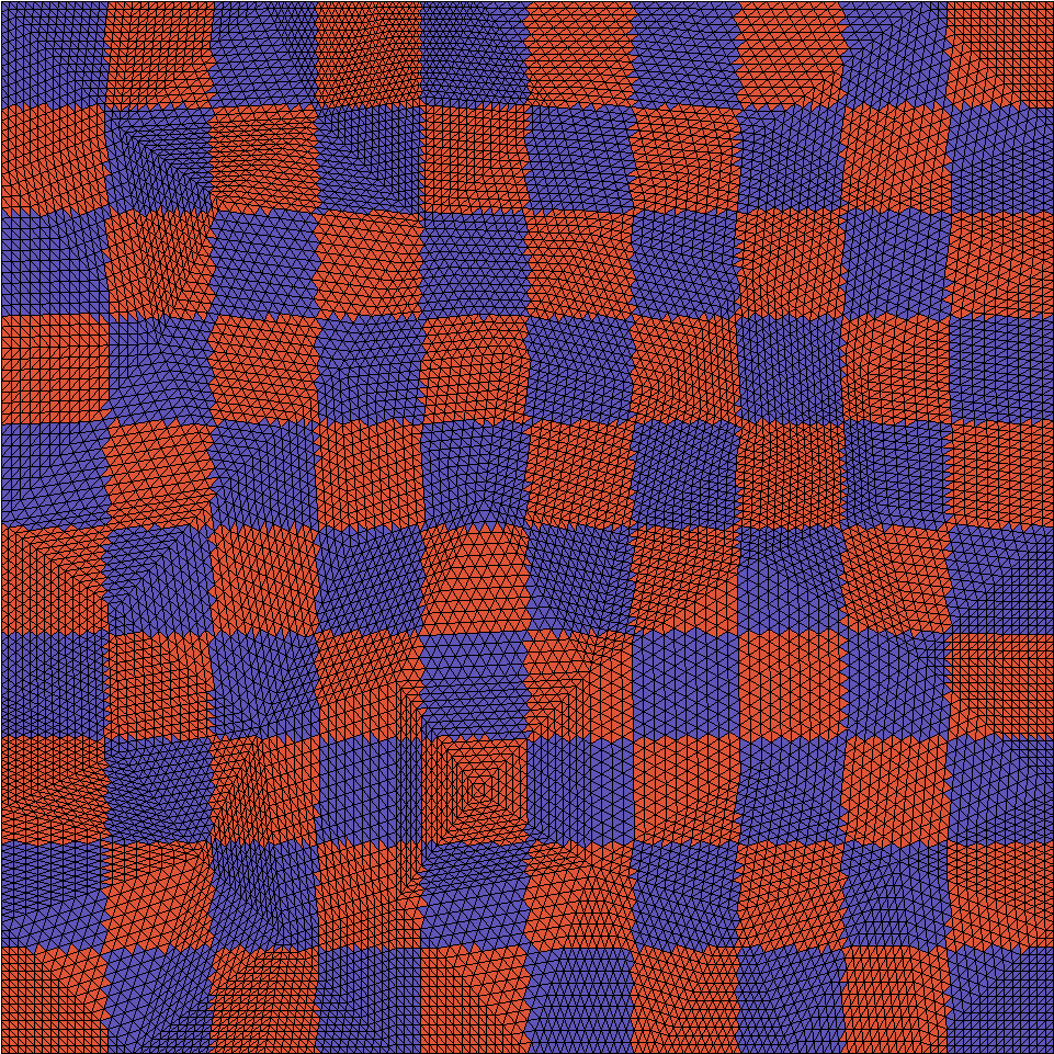
In this section, we present a number of tests that illustrate the robustness of the two–level methods with the polynomial smoother analyzed in the present paper all in accordance with Theorem 4.6. We consider the second order elliptic equation (4.15) with a mixture of Neumann and Dirichlet boundary conditions. The Dirichlet boundary conditions are imposed on the “east” and “west” vertical boundaries, i.e. $\displaystyle\Gamma_{D}=\Gamma_{E}\cup\Gamma_{W}$ of $\displaystyle\Omega$. As we pointed out, the coefficient $\displaystyle\alpha(\bm{x})$ is piecewise constant and we assume that the fine triangulation of $\displaystyle\Omega$ is aligned with (resolves) all the coefficient discontinuities. In Fig. 1 we show an example of a fine grid $\displaystyle\mathcal{T}_{h}$, aligned with discontinuities.

Figure 1. Checkerboard coefficient distribution on a mesh with $\displaystyle 25600$ elements and $\displaystyle 13041$ vertices.

5.1. Coarse spaces

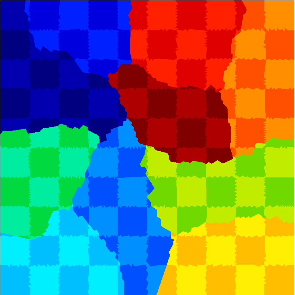
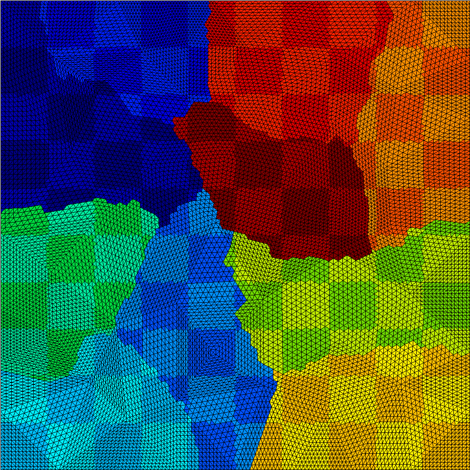
We use element agglomeration to define “coarse elements” as illustrated in Fig. 2. and a variant of the spectral AMGe method (see, e.g. [9]) in the form presented in [7].

(a)

(b)

Figure 2. (a) An example of $\displaystyle 10$ aggregates; (b) the corresponding element agglomerates (unions of fine grid elements) constructed on a mesh with $\displaystyle 6400$ elements and $\displaystyle 3321$ vertices. The distribution of discontinuity of the PDE coefficient is not resolved by the agglomerates.

Briefly the main steps in such coarse space construction are:

• Partitioning of the degrees of freedom as a union of non-overlapping sets, $\displaystyle\{{\mathcal{A}}\}$ called aggregates. This is achieved by first partitioning the set of elements into agglomerated elements $\displaystyle\{\tau\}$ (union of fine-grid elements). We use graph partitioner (metis) applied to the graph having vertices the fine-grid elements with edges between two elements if they share a common interface. Then, we form aggregates $\displaystyle{\mathcal{A}}$, where each aggregate (a set of fine degrees of freedom) corresponds a unique agglomerated element $\displaystyle\tau=\tau_{{\mathcal{A}}}$ by distributing the shared fine degrees of freedom (fine-grid element vertices belonging to two or more agglomerated elements) to a unique aggregate.

• Constructing a tentative interpolation matrix $\displaystyle{\overline{P}}$, defined for an agglomerate $\displaystyle\tau$. Consider the local generalized eigenproblem,

  $$A_{\tau}\bm{\varphi}_{k}=\theta_{k}D_{\tau}\bm{\varphi}_{k},$$

  where $\displaystyle A_{\tau}$ is the local stiffness matrix corresponding to the agglomerated element $\displaystyle\tau$, $\displaystyle D_{\tau}$ is its diagonal and $\displaystyle\theta_{1}\leq\theta_{2}\leq\ldots\leq\theta_{n_{{\mathcal{A}}}}$ with $\displaystyle n_{{\mathcal{A}}}=|{\mathcal{A}}|$ (cardinality of $\displaystyle{\mathcal{A}}$). Given a spectral tolerance $\displaystyle\theta$, we select the eigenvectors $\displaystyle\{\varphi_{k}\}_{k=1}^{n_{\theta}}$, where $\displaystyle n_{\theta}$ is the largest integer for which the inequality $\displaystyle\theta_{n_{\theta}}<\theta$ holds. Extended by zero outside each $\displaystyle{\mathcal{A}}$, the vectors $\displaystyle\{\bm{\varphi_{k}}\}_{k=1}^{n_{\theta}}$ form $\displaystyle n_{\theta}$ columns of the global tentative interpolation operator $\displaystyle{\overline{P}}$.

• Constructing the coarse space as the range of the interpolation matrix $\displaystyle P$, which is defined as

  $$P=s_{m}\left(\lambda^{-1}D^{-1}A\right){\overline{P}}.$$

  Here, as in the previous section, $\displaystyle D$ is the diagonal of $\displaystyle A$, $\displaystyle\lambda\geq\|D^{-\frac{1}{2}}AD^{-\frac{1}{2}}\|$ (e.g. $\displaystyle\lambda=\|D^{-1/2}AD^{-1/2}\|_{\infty}$), and $\displaystyle s_{m}(t)$ is the smoothed aggregation (SA) polynomial (cf., e.g., [8])

  $$s_{m}(t)=\frac{(-1)^{m}}{(2m+1)}\;\frac{T_{2m+1}(\sqrt{t})}{\sqrt{t}}.$$

5.2. Numerical tests

We recall some of the notations and definitions which are used in the tables and figures in this section.

• $\displaystyle N$ is the number of fine grid degrees of freedom;

• $\displaystyle N_{H}$ is the number of coarse degrees of freedom;

• $\displaystyle nnz(X)$ is the number of the nonzero elements in a matrix $\displaystyle X$;

• $\displaystyle{\widetilde{\varrho}}_{TG}$ is the asymptotic convergence factor of the two grid method;

• $\displaystyle oc(B)$ is the operator complexity measure of the two-grid preconditioner $\displaystyle B$, defined as $\displaystyle oc(B)=\frac{nnz(A)+nnz(A_{H})}{nnz(A)}$.

The first set of experiments are on a mesh with $\displaystyle 102,400$ elements and $\displaystyle N=51,681$ vertices using $\displaystyle 300$ agglomerated elements (AEs). We stop the iterations when the relative preconditioned residual norm is reduced by a factor of $\displaystyle\varepsilon=10^{-8}$. The piecewise constant coefficient $\displaystyle\alpha(\bm{x})$ is distributed in a checkerboard fashion with values $\displaystyle 1$ and $\displaystyle 10^{6}$ as illustrated in Fig. 1.

The experiments are performed for $\displaystyle m=2,4,6,8$, $\displaystyle a\equiv\frac{1}{\kappa}=0.158,0.085,0.055,0.04$, and $\displaystyle a=0.2,0.1,0.08,0.06$ respectively. They are chosen such that the inequality (3.8) (with $\displaystyle\omega=1$) holds:

$$\left(\frac{\sqrt{\kappa}-1}{\sqrt{\kappa}+1}\right)^{m}=\left(\frac{1-\sqrt{a}}{1+\sqrt{a}}\right)^{m}<\frac{a}{1-a}=\frac{1}{\kappa-1},\quad a=\frac{1}{\kappa}.$$

The same degree $\displaystyle m$ is used for the polynomial smoother in the two-level algorithm and the smoother of the tentative interpolation matrix (it is smoothed out by $\displaystyle s_{m}\left(D^{-1}A\right)$). The number of non-zero entries of $\displaystyle A$, is $\displaystyle nnz(A)=359,841$. We also show how the spectral tolerance $\displaystyle\theta$ and the polynomial degree $\displaystyle m$ influences the convergence versus operator complexity. The results are presented in Tables 1–4. It is evident from the results that the method can become fairly fast (in terms of convergence factors) at the expense of large operator complexity.

				$\displaystyle\widetilde{\rho}_{TG}$
$\displaystyle\theta$	$\displaystyle N_{H}$	$\displaystyle nnz(A_{H})$	$\displaystyle oc(B)$	$\displaystyle a=0.158$	$\displaystyle a=0.2$
0.010	774	15,930	1.04	0.995	0.995
0.077	3,629	342,515	1.95	0.879	0.889
0.149	6,557	1,115,207	4.10	0.393	0.492

Table 1. Two-grid convergence, $\displaystyle m=2$.

				$\displaystyle\widetilde{\rho}_{TG}$
$\displaystyle\theta$	$\displaystyle N_{H}$	$\displaystyle nnz(A_{H})$	$\displaystyle oc(B)$	$\displaystyle a=0.085$	$\displaystyle a=0.1$
0.010	774	22,092	1.06	0.985	0.986
0.077	3,629	472,907	2.31	0.531	0.538
0.149	6,557	1,538,845	5.28	0.188	0.084

Table 2. Two-grid convergence when $\displaystyle m=4$.

				$\displaystyle\widetilde{\rho}_{TG}$
$\displaystyle\theta$	$\displaystyle N_{H}$	$\displaystyle nnz(A_{H})$	$\displaystyle oc(B)$	$\displaystyle a=0.055$	$\displaystyle a=0.08$
0.010	774	29,448	1.08	0.965	0.969
0.077	3,629	636,671	2.78	0.205	0.179
0.149	6,557	2,074,291	6.76	0.202	0.026

Table 3. Two-grid convergence when $\displaystyle m=6$.

				$\displaystyle\widetilde{\rho}_{TG}$
$\displaystyle\theta$	$\displaystyle N_{H}$	$\displaystyle nnz(A_{H})$	$\displaystyle oc(B)$	$\displaystyle a=0.04$	$\displaystyle a=0.06$
0.010	774	37,618	1.10	0.926	0.933
0.077	3,629	808,357	3.25	0.197	0.111
0.149	6,557	2,632,755	8.32	0.193	0.028

Table 4. Two-grid convergence when $\displaystyle m=8$.

In the last experiment shown in Table 5, we illustrate the behavior of the method with respect to varying the contrast $\displaystyle 10^{c}$ again distributed in a checkerboard fashion. As it is clearly seen, the two-grid method exhibits very good uniform two-grid convergence with operator complexity less than two.

$\displaystyle c$	-12	-9	-6	-3	0	3	6	9	12
$\displaystyle N_{H}$	2336	2336	2336	2339	2322	2322	2322	2322	2322
$\displaystyle oc(B)$	1.94	1.94	1.94	1.94	1.93	1.93	1.93	1.93	1.93
$\displaystyle n_{it}$	17	17	17	17	17	16	16	16	16
$\displaystyle\widetilde{\rho}_{TG}$	0.219	0.219	0.219	0.219	0.219	0.200	0.198	0.197	0.198

Table 5. Contrast independent two-grid convergence; coefficient jumps are $\displaystyle 10^{c}$. The method corresponds to spectral threshold $\displaystyle\theta=0.045$, $\displaystyle m=8$, and $\displaystyle a=0.04$.

Appendix A

The proof of Theorem 2.1 presented in this section is based on an equivalent result given in [1, p. 33, Equation (4.25)]. Let us also remark that in this section our considerations are on the interval $\displaystyle[-1,1]$ and in addition, by best polynomial approximation we mean the best polynomial approximation in the norm $\displaystyle\|\cdot\|_{\infty}$ on $\displaystyle[-1,1]$.

A.1. An approximation result equivalent to Theorem 2.1

We now formulate the result in [1] in the notation introduced earlier and show how the result in Theorem 2.1 can be derived from [1, p. 33, Equation (4.25)].

Theorem A.1 (G. Meinardus, [1]).

The polynomial $\displaystyle\widetilde{Q}_{m}\in\mathcal{P}_{m}$, of degree less than or equal to $\displaystyle m$, which furnishes the best approximation to $\displaystyle\frac{1}{t-a}$, $\displaystyle a>1$ on $\displaystyle[-1,1]$ is given by:

$$\widetilde{Q}_{m}(t)=\frac{1}{t-a}\left(1-\frac{(a-\sqrt{a^{2}-1})^{m}}{a^{2}-1}\widetilde{R}_{m+1}(t)\right),$$

where

$$\widetilde{R}_{m+1}(t)=\left[(at-1)T_{m}(t)+\frac{\sqrt{a^{2}-1}}{m}(t^{2}-1)T_{m}^{\prime}(t)\right].$$

The result we have just stated is for the best approximation to the function $\displaystyle\frac{1}{t-a}$, while to prove Theorem 2.1 we need such result for $\displaystyle\frac{1}{t+a}$. It is however easy to show that Theorem A.1 also provides the best polynomial approximation to $\displaystyle\frac{1}{t+a}$. Indeed, note that for any polynomial $\displaystyle p(t)$ of degree less than or equal to $\displaystyle m$, and for all $\displaystyle t\in[-1,1]$, there holds

$$p(-t)-\frac{1}{(-t)-a}=-\left(-p(-t)-\frac{1}{t+a}\right).$$

Further, for a function $\displaystyle g(t)$ continuous on $\displaystyle[-1,1]$ we also have,

$$\max\{g(t)~{}|~{}t\in[-1,1]\}=\max\{g(-t)~{}|~{}t\in[-1,1]\},$$

These two identities give that

$$\left\|p-\frac{1}{t-a}\right\|_{\infty}=\max_{t\in[-1,1]}\left|p(-t)-\frac{1}{(-t)-a}\right|=\max_{t\in[-1,1]}\left|(-p(-t))-\frac{1}{t+a}\right|.$$

Since $\displaystyle p$ was an arbitrary polynomial of degree less than or equal to $\displaystyle m$, we may take the infimum over all $\displaystyle p\in\mathcal{P}_{m}$. According to Theorem A.1 the left side is minimized for $\displaystyle p(t)=\widetilde{Q}_{m}(t)$. Therefore the right side should also be minimized for $\displaystyle p(t)=\widetilde{Q}_{m}(t)$. More precisely, we have

(A.1) $$\left\|(-\widetilde{Q}_{m}(-t))-\frac{1}{t+a}\right\|_{\infty}=\inf_{p\in\mathcal{P}_{m}}\max_{t\in[-1,1]}\left|(-p(-t))-\frac{1}{t+a}\right|=\inf_{q\in\mathcal{P}_{m}}\left\|q-\frac{1}{t+a}\right\|_{\infty},$$

which shows that the best polynomial approximation to $\displaystyle\frac{1}{t+a}$ on $\displaystyle[-1,1]$ is $\displaystyle(-\widetilde{Q}_{m}(-t))$.

A.2. Proof of Theorem 2.1

We need to show that for the polynomial $\displaystyle Q_{m}(t)$ defined as in (2.6) we have $\displaystyle Q_{m}(t)=(-\widetilde{Q}_{m}(-t))$. We use properties of Chebyshev polynomials to prove this identity. If we set $\displaystyle\alpha=\arccos t$ we have

$$\displaystyle(t^{2}-1)T^{\prime}_{m}(-t) \displaystyle= \displaystyle(-1)^{m}m\sin\alpha\sin m\alpha=\frac{(-1)^{m-1}m}{2}(\cos(m+1)\alpha-\cos(m-1)\alpha)$$

$$\displaystyle= \displaystyle\frac{(-1)^{m-1}m}{2}(T_{m+1}(t)-T_{m-1}(t)).$$

Recall that $\displaystyle T_{k}(-t)=(-1)^{k}T_{k}(t)$, $\displaystyle\delta=(a-\sqrt{a^{2}-1})$, and $\displaystyle 2tT_{m}(t)=(T_{m+1}(t)+T_{m-1}(t))$. Therefore, we have

$$\displaystyle\widetilde{R}_{m+1}(-t) \displaystyle= \displaystyle-(at+1)T_{m}(-t)+\frac{\sqrt{a^{2}-1}}{m}(t^{2}-1)T_{m}^{\prime}(-t)$$

$$\displaystyle= \displaystyle(-1)^{m+1}(at+1)T_{m}(t)+\frac{(-1)^{m-1}\sqrt{a^{2}-1}}{2}(T_{m+1}(t)-T_{m-1}(t))$$

$$\displaystyle= \displaystyle\frac{(-1)^{m+1}}{2}\left[(a(T_{m+1}(t)+T_{m-1}(t))+2T_{m}(t)+\sqrt{a^{2}-1}(T_{m+1}(t)-T_{m-1}(t))\right]$$

$$\displaystyle= \displaystyle\frac{(-1)^{m+1}}{2}\left[\delta^{-1}T_{m+1}(t)+2T_{m}(t)+\delta T_{m-1}(t)\right]$$

$$\displaystyle= \displaystyle\frac{(-1)^{m}}{2}\left[\eta^{-1}T_{m+1}(t)-2T_{m}(t)+\eta T_{m-1}(t)\right].$$

Looking at the definition of $\displaystyle R_{m+1}(t)$, given in Theorem 2.1 (relation (2.7)) it is easily seen that $\displaystyle\widetilde{R}_{m+1}(-t)=\frac{(-1)^{m}}{2}R_{m+1}(t)$. Since $\displaystyle(\eta^{-1}-\eta)^{2}=4(a^{2}-1)$, we finally get

$$\displaystyle(-\widetilde{Q}_{m}(-t)) \displaystyle= \displaystyle-\frac{1}{-t-a}\left(1-\frac{4\delta^{m}}{(\delta+\delta^{-1})^{2}}\widetilde{R}_{m+1}(-t)\right)=\frac{1}{t+a}\left(1-\frac{2(-1)^{m}\delta^{m}}{(\delta^{-1}-\delta)^{2}}R_{m+1}(t)\right)$$

$$\displaystyle= \displaystyle\frac{1}{t+a}\left(1-\frac{2\eta^{m}}{(\eta-\eta^{-1})^{2}}R_{m+1}(t)\right)=Q_{m+1}(t).$$

Thus, $\displaystyle Q_{m}(t)$ and $\displaystyle(-\widetilde{Q}_{m}(-t))$ coincide and the proof is complete. $\displaystyle\Box$

Remark A.2.

It is also possible to prove directly that the polynomial in (2.6) is a polynomial of best approximation to $\displaystyle x^{-1}$ by specifying the points of Chebyshev alternance. Such proof is however much more elaborate than the one presented here.

References

- [1] G. Meinardus. Approximation of functions: Theory and numerical methods. Expanded translation of the German edition. Translated by Larry L. Schumaker. Springer Tracts in Natural Philosophy, Vol. 13. Springer-Verlag New York, Inc., New York, 1967.
- [2] T. J. Rivlin. An introduction to the approximation of functions. Dover Publications Inc., New York, 1981. Corrected reprint of the 1969 original, Dover Books on Advanced Mathematics.
- [3] P. L. Chebyshev. Sur les polynômes réprésentant le mieux les valeurs des fonctions fractionnaires élémentaires pour les valeurs de la variable contenues entre deu limites données. In Oeuvres, volume II, pages 669–678. St Petersburg, 1907.
- [4] Juan Galvis and Yalchin Efendiev. Domain decomposition preconditioners for multiscale flows in high-contrast media. Multiscale Modeling & Simulation, 8(4):1461–1483, 2010.
- [5] Robert Scheichl, Panayot S. Vassilevski, and Ludmil T. Zikatanov. Weak approximation properties of elliptic projections with functional constraints. Multiscale Modeling & Simulation, 9(4):1677–1699, 2011.
- [6] Marian Brezina, Caroline Heberton, Jan Mandel, and Petr Vaněk. An iterative method with convergence rate chosen a priori. Technical Report 140, University of Colorado Denver, CCM, University of Colorado Denver, April 1999. An earlier version presented at the 1998 Copper Mountain Conference on Iterative Methods, April 1998.
- [7] M. Brezina and P. S. Vassilevski. Smoothed aggregation spectral element agglomeration AMG: SA-AMGe. Technical Report LLNL-PROC-490083, Lawrence Livermore National Laboratory, June 29 2011. To appear in Proceedings of the 8th International Conference on ”Large-Scale Scientific Computations”, Sozopol, Bulgaria, June 6, 2011 through June 10, 2011.
- [8] M. Brezina, P. Vaněk, and P. S. Vassilevski. An improved convergence analysis of smoothed aggregation algebraic multigrid. Numerical Linear Algebra with Applications, pages n/a–n/a, 2011.
- [9] P. S. Vassilevski. Multilevel block factorization preconditioners. Springer, New York, 2008. Matrix-based analysis and algorithms for solving finite element equations.
- [10] R. D. Falgout, P. S. Vassilevski, and L. T. Zikatanov. On two-grid convergence estimates. Num. Lin. Alg. Appl., 12:471–494, 2005. Also available as LLNL technical report UCRL-JC-150807.