Detecting circumbinary planets using eclipse timing of binary stars - numerical simulations

Abstract

The presence of a body in an orbit around a close eclipsing binary star manifests itself through the light time effect influencing the observed times of eclipses as the close binary and the circumbinary companion both move around the common centre of mass. This fact combined with the periodicity with which the eclipses occur can be used to detect the companion. Given a sufficient precision of the times of eclipses, the eclipse timing can be employed to detect substellar or even planetary mass companions.

The main goal of the paper is to investigate the potential of the photometry based eclipse timing of binary stars as a method of detecting circumbinary planets. In the models we assume that the companion orbits a binary star in a circular Keplerian orbit. We analyze both the space and ground based photometry cases. In particular, we study the usefulness of the on-going COROT and Kepler missions in detecting circumbinary planets. We also explore the relations binding the planet discovery space with the physical parameters of the binaries and the geometrical parameters of their light curves. We carry out detailed numerical simulations of the eclipse timing by employing a relatively realistic model of the light curves of eclipsing binary stars. We study the influence of the white and red photometric noises on the timing precision. We determine the sensitivity of the eclipse timing technique to circumbinary planets for the ground and space based photometric observations. We provide suggestions for the best targets, observing strategies and instruments for the eclipse timing method. Finally, we compare the eclipse timing as a planet detection method with the radial velocities and astrometry.

1 Introduction

Accurate light curves of eclipsing binary stars can be used to precisely measure the times of eclipses. Such eclipse timing measurements (ET) can then be compared with the predicted ones and used to infer information on e.g. the presence of an additional body orbiting the eclipsing binary. The presence of an additional body will cause the motion of the eclipsing binary with respect to the centre of mass of the entire system and result in advances/delays in the times of eclipses due to the light time effect. This old idea (it dates back to XVII century and Ole Roemer) has been used to e.g. detect stellar companions to eclipsing binaries. It can also be used to detect circumbinary planets (P-type planets, Dvorak 1984). Clearly, this idea is simple and has already been explored in the literature as a potential way of detecting extrasolar planets (see e.g. Muterspaugh et al., 2007; Doyle & Deeg, 2004; Deeg et al., 2008).

In this paper, we carry out detailed numerical simulations of ET to explore in more depth what can be achieved with this technique both from the ground and space. In the first part, we study the CoRoT and Kepler and investigate how their very high photometric precision (Alonso et al., 2008; Koch et al., 2004) can be used to detect circumbinary planets via ET. In the second part, we estimate the influence of the red noise and the gaps in the light curves typical for the ground based photometry caused by e.g. the day-night cycle, technical problems and weather conditions on the discovery space.

In section 2 we describe the light curve and noise models used in the simulations, in section 3 we describe how a planetary timing signal is generated and detected in a simulated light curve, in section 4 we analyze the space missions CoRoT and Kepler, in section 5 we discuss a ground based effort and conclusions are provided in section 6.

2 Light curve of an eclipsing binary and its noise

The model of an eclipsing binary is from Nelson & Davis (1972). It describes systems that do not fill their Roche lobes. We decided to examine detached binaries as such systems are the most likely ones to serve as stable clocks. The adopted model is simple enough to provide fast computations and at the same time enables an adequate description of an eclipsing binary. Eclipses are described as an obscuration of two discs. The algorithm used to compute a synthetic light curve comes from Nelson & Davis (1972) and is based on a few simple equations. Let us note that two of the equations are misprinted in Nelson & Davis (1972). The correct version for the eclipsed surface is

$$B=r_{1}^{2}\arccos{\frac{r_{1}-a}{r_{1}}}-(r_{1}-a)(2r_{1}a-a^{2})^{1/2}$$ (1)

$$\qquad+r_{2}^{2}\arccos{\frac{r_{2}-b}{r_{2}}}-(r_{2}-b)(2r_{2}b-b^{2})^{1/2}$$

for the situation shown in Fig. 1 when the projected stars’ separation is larger than radius of the bigger star and

$$B=\pi r_{1}^{2}-r_{1}^{2}\arccos{\frac{r_{1}-a}{r_{1}}}+(r_{1}-a)(2r_{1}a-a^{2})^{1/2}$$ (2)

$$+r_{2}^{2}\arccos{\frac{r_{2}-b1}{r_{2}}}-(2r_{2}b-b^{2})^{1/2}$$

for the situation shown in Fig. 2. In the above $B$ is the obscured surface, $r_{1}$, $r_{2}$ denote the radius of the first and second star, $a$, $b$ are shown in Fig. 2 and $\cos\alpha=\frac{r_{2}-b}{r_{2}}$, $\cos\Psi=\frac{r_{1}-a}{r_{1}}$. The remaining symbols are as in the original article.

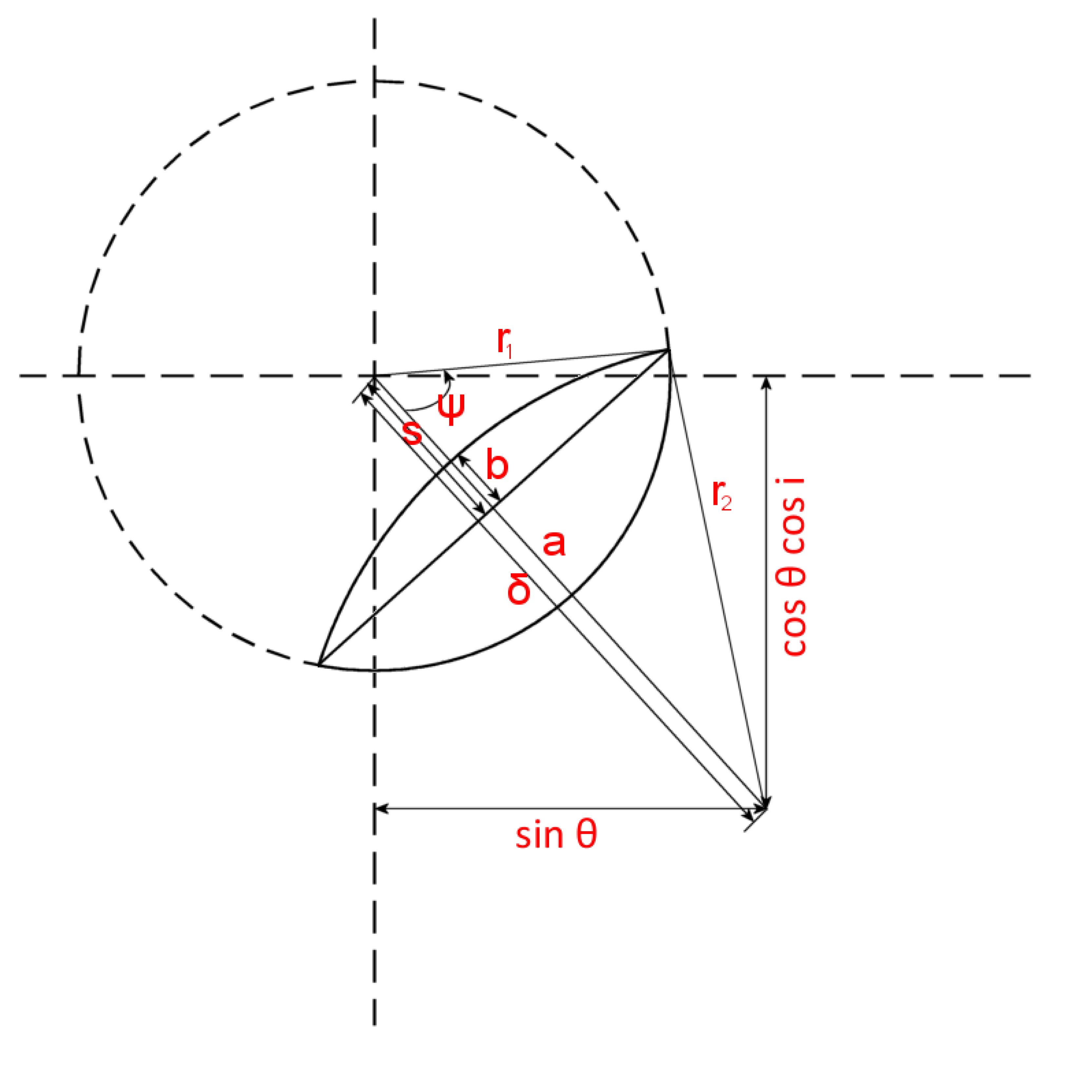
Figure 1: The first type of an occultation when the projected stars’ separation is larger than the radius of the bigger star. The symbols are described in the text and in Nelson & Davis 1972.

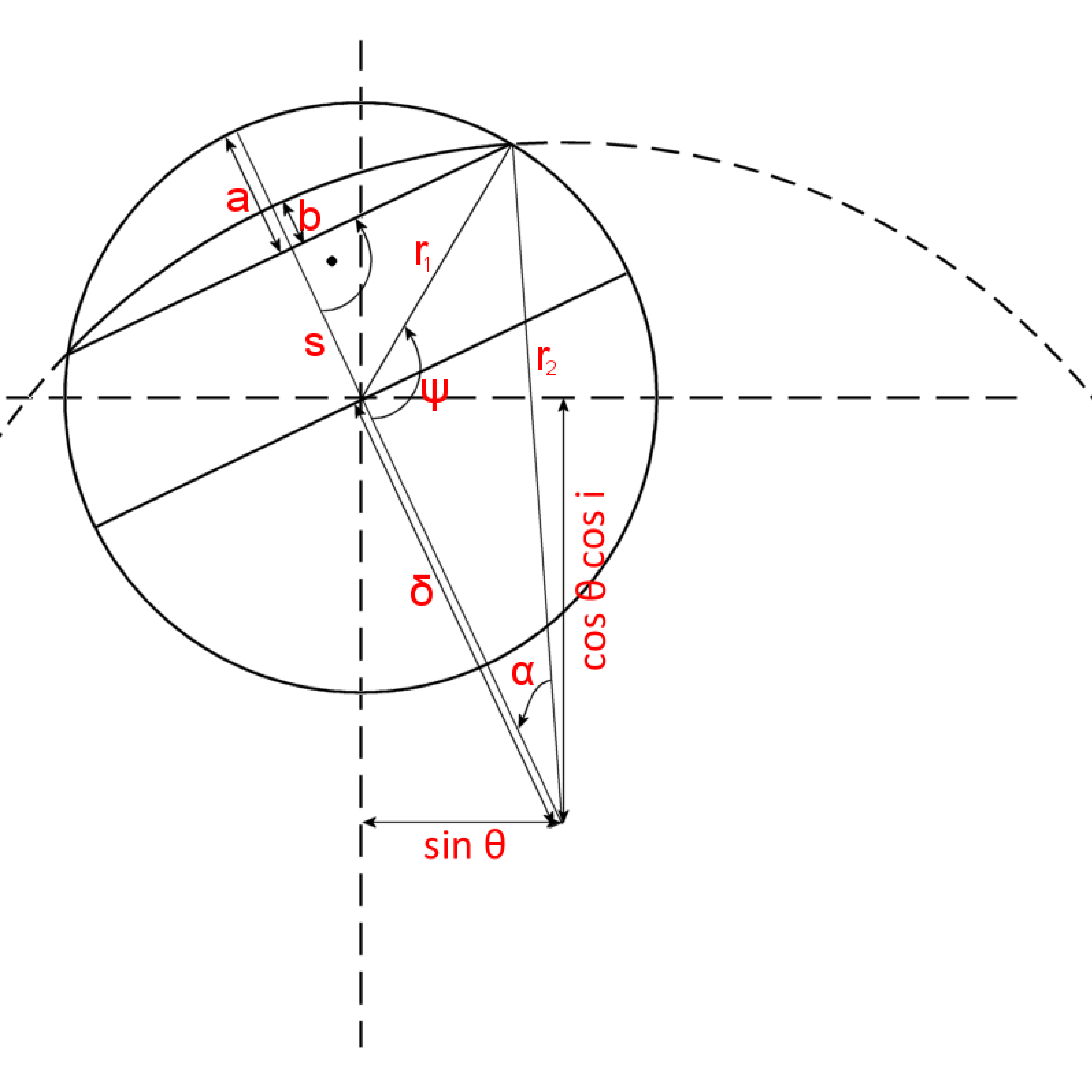
Figure 2: The second type of an occultation, the projected stars’ separation is smaller than the radius of the bigger star.

In the above description, the local perspective effect is ignored. In a typical realistic case the separation between the stars is very small compared to the distance between the observer and binary. The parameters describing the system are the separation $a$, radius of the first and second star $r_{1}$, $r_{2}$, the total luminosity $L$, the fraction of light emitted by second component $L_{2}$, the Keplerian elements of the planetary and binary orbits (ellipticity, inclination, semi major axis). Both orbits, of the planet and the binary star are Keplerian. We assume that the perturbing planet changes only the position of the binary stars’ centre of mass and none of the orbital elements. In our simulations we assume circular orbits.

In general we add three types of noise to the synthetic light curves. The first one is the photon noise depending on the brightness of an observed eclipsing binary, the second one is the white noise of different origin than the photon noise and the third one is the red noise due to e.g. the Earth’s atmosphere, the instrumentation. The first two are typical for the space based photometry and all three are expected to be present in the ground based data.

The red noise is applied using the package for the exact numerical simulation of power-law noises PLNoise (Milotti, 2006, 2007). It is worth noting that the impact of the red noise on the planet discovery space differs with the typical time scale associated with the red noise. In our code the red noise is parameterized via the minimal decay rate of the oscillators generating the noise. Even if the standard deviation remains the same, the eclipses timing precision changes with the typical time scale of the red noise. The examples of red noise with different time scales are shown in Figure 3.

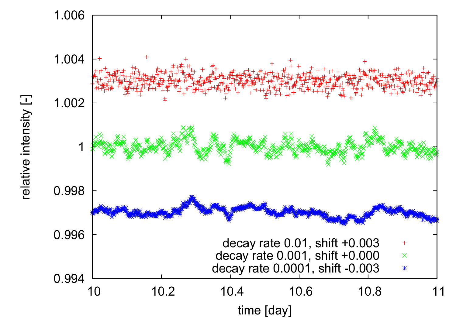
Figure 3: Three examples of the red noise with the same standard deviation and different decay rates $\lambda_{\mathrm{min}}$ of 0.01, 0.001 and 0.0001. Red noise used in our simulations of ground observations is characterized by $\lambda_{\mathrm{min}}=$ 0.01.

3 Planet discovery space

We simulate a light curve of an eclipsing binary with the photon noise dependent on the brightness of a target and additional Gaussian and red noises if necessary. The level of the last two is based on the instrument’s characteristic and the place of the observations (space/ground). For such a light curve, a planetary light time disturbance affecting the times of photometric measurements is also added according to the assumed orbital parameters of a circumbinary planet.

The criterion for a detection or a non detection of a planet is as follows

$$w_{j}=\frac{1}{\sigma_{x,j}^{2}},\quad\overline{x}_{w}=\frac{\sum_{j=1}^{L}w_{j}x_{j}}{\sum_{j=1}^{L}w_{j}},\\$$ (3)

$$\sigma_{S}=\sqrt{\frac{\sum_{j=1}^{L}(\overline{x}_{w}-x_{j})^{2}}{L-1}}\geq 3max(\sigma_{x,1},\dots,\sigma_{x,L})$$ (4)

where $x_{j}$ is the measured time of the $j$-th eclipse (the $t_{0}$ moment of one complete light curve), $\sigma_{x,j}$ denotes its standard deviation and $w_{j}$ the corresponding weight of such a timing measurement. Finally $\sigma_{S}$ is calculated to estimate the magnitude of the timing signal which is present in data and this is compared to the largest error of $x$. Such a procedure allows us to get a quick insight whether a planetary timing signature may be present in the data set. If the inequality 4 is satisfied it means that a planet is detected and this is denoted with red colour. Otherwise, a non detection is denoted with blue colour. The resulting discovery space is a result of an averaging over a rectangle of 121 neighbouring points. Pure red colour denotes a certain detection (fraction 121/121) and pure blue colour a certain non-detection. Intermediate colours are computed as a linear interpolation between the two basic colours according to a given fraction of detections in a rectangle (see Figure 4).

Note that such a definition of the detection means that a planetary signal is detected when its timing amplitude $A$ is equal to or larger than $\sim 4\sigma$ where $\sigma$ is the precision (formal error) of the timing accuracy. Hence, the main factor that defines the discovery space is the precision with which one can measure the moment of one eclipse. Obviously, the longer the data set of timing measurements, the higher is the confidence level with which a planetary signal is detected (for details see Cumming, 2004). For example, since Kepler will provide $\sim$10 times longer data sets than CoRoT, the confidence level of its putative detection would be higher. Or in other words, for the same confidence level Kepler would allow for a detection of smaller amplitudes than CoRoT. We have decided to use our simpler, more conservative approach which is not affected by a particular choice of sampling of the timing measurements.

In the above, the time of an eclipse is computed in two ways. The first and classic approach is to use $x_{j}$ as one of the parameters of a multiparameter least-squares fit of a physical model to the synthetic light curve. In this approach the parameters of the binary assumed to calculate the light curve are disturbed and used as the starting values of the least-squares parameters. Parameters which are varied and then fitted for include the radii $r_{1}$, $r_{2}$, the inclination $i$, $t_{0}$ the orbital reference epoch, the orbital period of the binary $P$ and the luminosity of the secondary $L_{s}$. We use MINPACK library (Moré et al., 1980, 1984) to carry out a least-squares fitting.

The simulations can be easily extended to e.g. cases with the elliptically distorted stars and include the limb darkening as e.g. in Nelson & Davis (1972). As we have tested, in such a case the results are slightly different after introducing these two effects and the total time required to compute a discovery space is a few times longer. The resulting area of the discovery space corresponding to detectable planets is a bit smaller and moves toward upper-right corner (see e.g. Figure 4). This is in our opinion the result of the correlations between the increasing number of parameters used in the least-squares fit which often accounts for very subtle effects. For this reason, we believe that it is best to use an approach known from e.g. radio pulsar timing and precision radial velocities relying on a reference template pulse or spectrum to measure a timing or RV shift.

In such an approach the time of an eclipse is computed by comparing a given light curve with a reference light curve obtained by folding all the simulated photometric measurements with the orbital period of a binary. As mentioned, this is an approach used in radio pulsar timing or in precision radial velocity technique where the cross correlation function and the reference radio pulse or template spectrum are used to compute a timing shift or a Doppler shift. In our case, in order to compute $x_{j}$ and its formal error $\sigma_{x,j}$ we use the least-squares formalism. Let us note that for the simpler light curve model with the spherical binary components and no limb darkening, both approaches result in the same discovery space and for the more complicated binary model case, the approach employing a reference light curve results in a better discovery space (a wider range of detectable planets). Obviously the second approach will work well only if the light curve is sufficiently stable but then only for such stable light curves/binaries one may hope to detect planets.

The parameters of the binary star, the instruments and the simulated photometric measurements are summarized in Tables 1, 2 and 3. The discovery space is computed on a dense grid of planetary periods and masses. For the figures, the discovery space is represented by averaging 121 neighbour points from the grid. The red colour in the diagrams denotes certain detection (fraction 121/121) and the blue one the lack of detection (0/121). All the intermediate colours are computed as a linear interpolation. Black lines in the discovery space show the planet’s mass and period which generates a given timing amplitude, $A$. The equation describing such a line is given by

$$M_{P}(P_{pl})=\left(\frac{4\pi^{2}M_{B}^{2}}{P_{pl}^{2}G}\right)^{\frac{1}{3}}\cdot(Ac)$$ (5)

where $M_{P}$, $P_{pl}$ are the mass and period of a planet, $M_{B}$ is the mass of the binary star, $c$ stands for the speed of light and $G$ is the gravitational constant.

Table 1: Binary’s star characteristic

Total luminosity	2 L☉
Secondary star luminosity	1 L☉
Total binary star mass	2 M☉
Effective temperature of binary components	5780 K
Orbital eccentricity	0
Radii	1 R☉
Orbital period	3 days
Inclination	90 deg
Orbit inclination of a planet	90 deg

Table 2: Instrument characteristic used in our simulations.

Parameter	CoRoT	Kepler	ground	Unit
White noise	0.07	0.02	0.35	mmag
Red noise	0	0	0.35	mmag
Band	370-950	430-890	502-587	nm
Integration time	320	900	varies	s
Observing window	150	1461	365	days
Aperture	588	2256	1963.5	cm2
Throughput	81	81	81	%
Target stars (transits)	12-15.5	9-14	-	mag
Target stars	6-9	-	-	mag
(stellar seismology)
Target stars	-	-	6-14	mag
(ET)

Table 3: Simulation’s internal parameters

Orbital period	from 10 days
Planet mass	from 0.05 MJupiter
Effective no. of simulation points	40401
No. of light curve active parts	varies
Red noise $dt$	1
Red noise $nt$	0.1
Red noise $\lambda_{\mathrm{min}}$	0.01
Red noise $\lambda_{\mathrm{max}}$	1

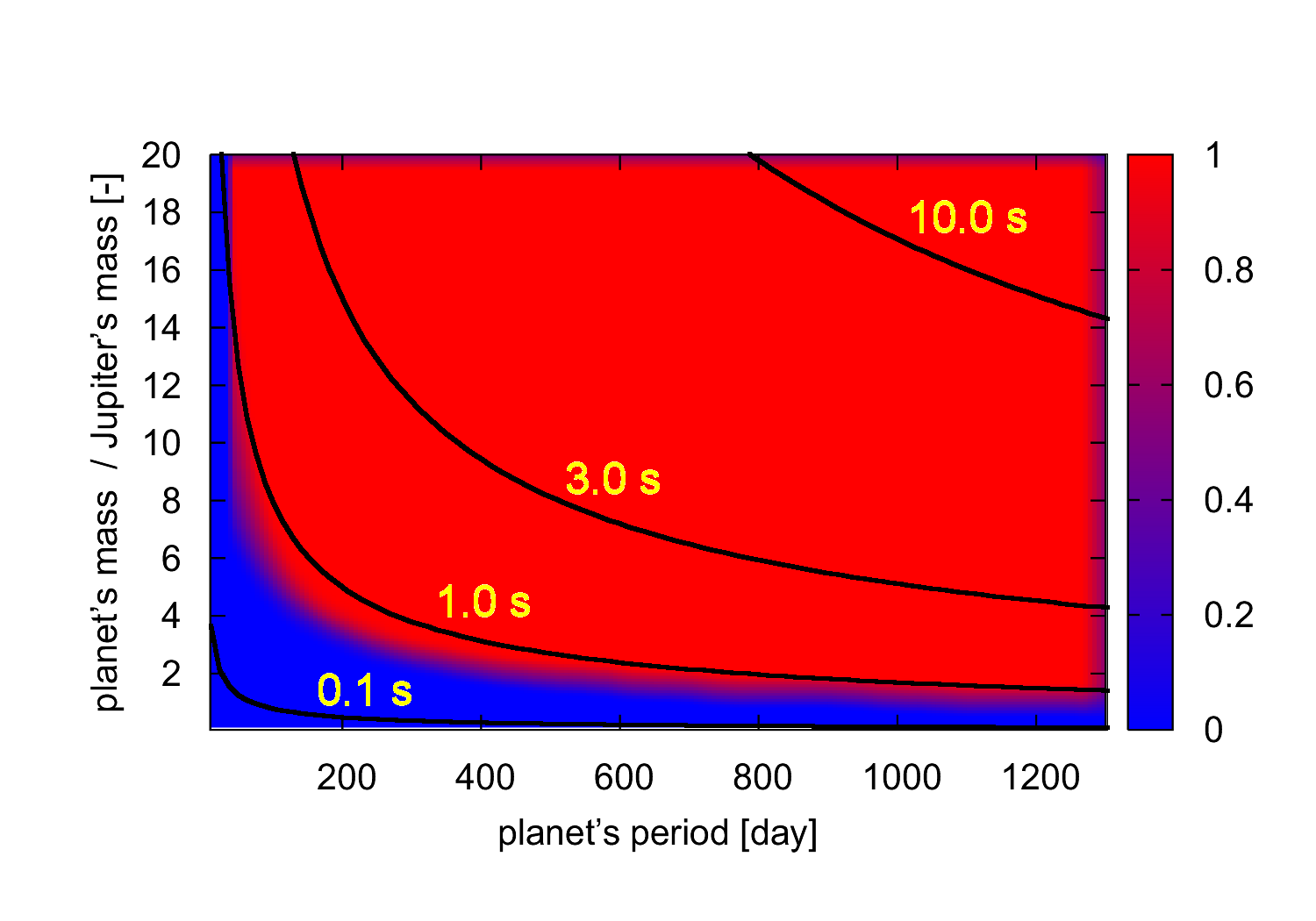
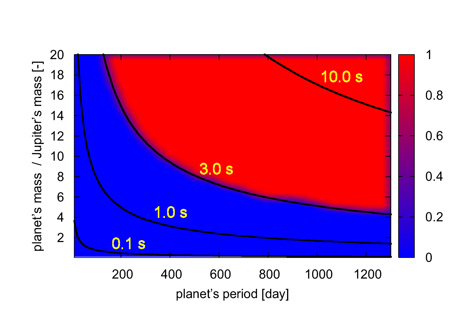
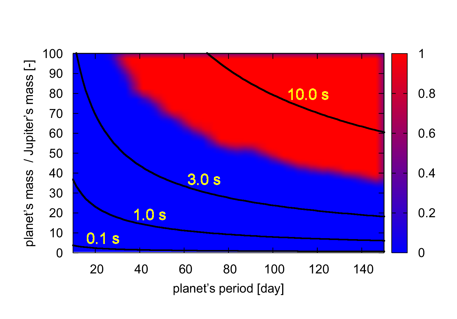
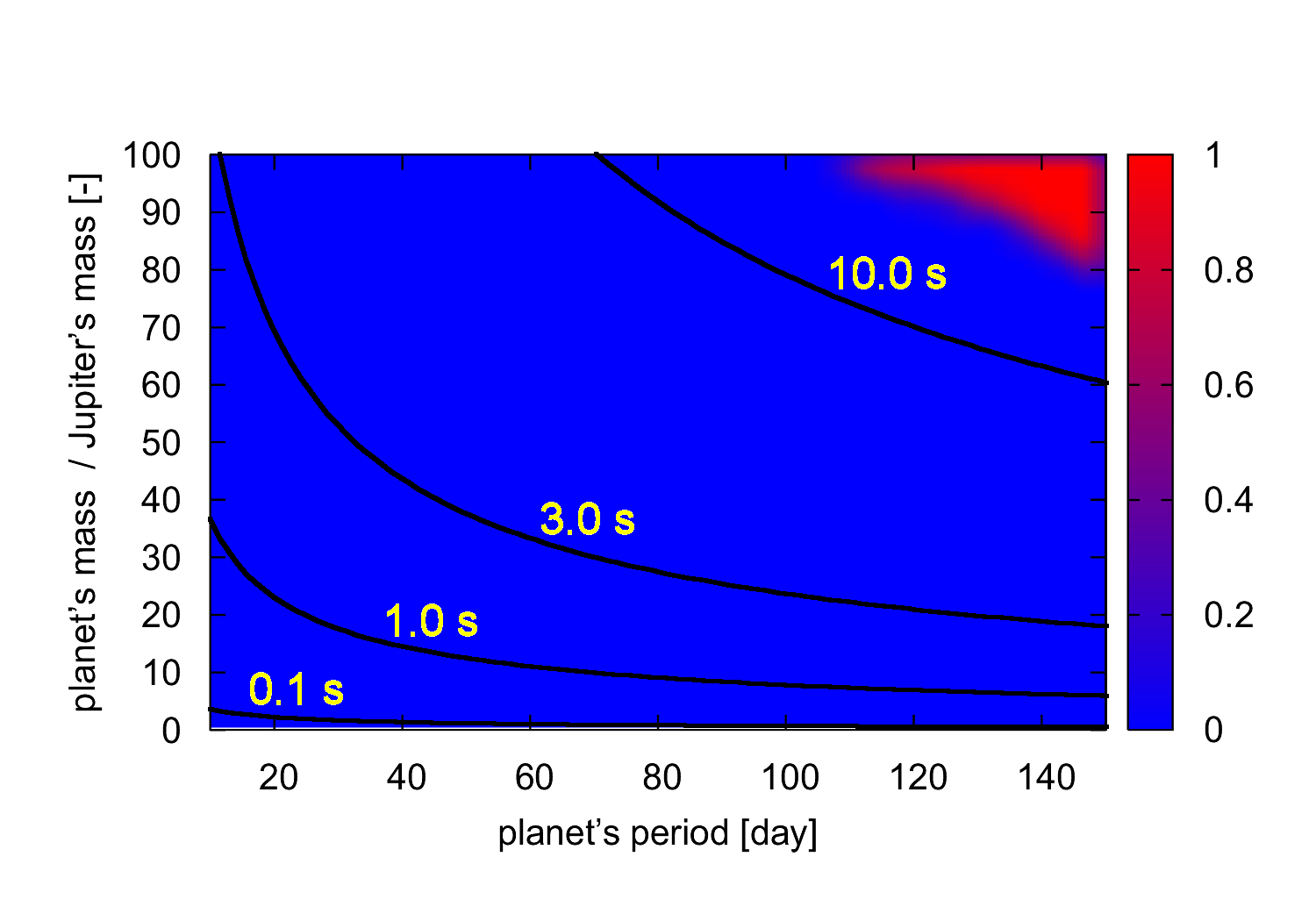
Figure 4: Typical discovery space for Kepler (top) and CoRoT (bottom). Top left for a 9 mag target (the photometric error is $\sigma=0.035$ mmag) and top right for a 14 mag target ($\sigma=0.17$ mmag). Bottom left for a 13 mag target ($\sigma=0.5$ mmag) and bottom right for a 15 mag target ($\sigma=1.5$ mmag). One should remember that a measurement is taken every 900 sec for Kepler which is in the middle of 30 minutes and 1 minute cadence now used and 320 sec for CoRoT hence the total number of measurements varies per one full orbital period of the target binary. Now Kepler uses 30 and 1 minute cadences but this does not affect the outcome of the simulations. For example longer integration times provide a smaller photometric error but also a smaller number of measurements per light curve.

Figure 4 shows a few examples of a typical discovery space for the CoRoT and Kepler missions. Each discovery space is a result of one simulation run covering 40401 points (201 by 201) for which the inequality Eq. 4 was checked. Based on a discovery space and Equation 5, we derive a timing amplitude which fits best to the border between a detection and non detection. As can be seen e.g. in Figure 4(a-b) $A$ is an approximation of the actual border and hence the best fit value of $A$ is also characterized by its non zero error $\sigma_{A}$ depending on how the real border deviates from $A$.

4 CoRoT and Kepler

The ongoing space missions CoRoT and Kepler aimed to detect transiting planets can in principle be used also to detect circumbinary planets via ET. These missions have the obvious advantage over any ground effort of providing an uninterrupted set of photometric measurements of a respectively 150 day and four year time span. In our simulations we used the parameters of the missions as described by Costes et al. (2004), Garrido & Deeg (2006) and Auvergne et al. (2009) for CoRoT and by Koch et al. (2004) for Kepler. They are also summarized in Table 2.

The examples of discovery space for CoRoT and Kepler are shown in Figure 4. While both instruments are capable of providing very precise photometry, the resulting discovery space is also affected by the cadence of photometric measurements and the brightness of the targets. Overall the potential of detecting circumbinary planets with CoRoT and Kepler comes out somewhat less attractive than one may have hoped for. The simulations allow us to determine the following relations for CoRoT $A(\sigma)=10.72~{}\sigma$, and for Kepler $A(\sigma)=19.14~{}\sigma$, $\sigma$ is the photometric precision of a single measurement in mmag and $A$ the detectable timing amplitude (DTA) is given in seconds (see Figure 5).

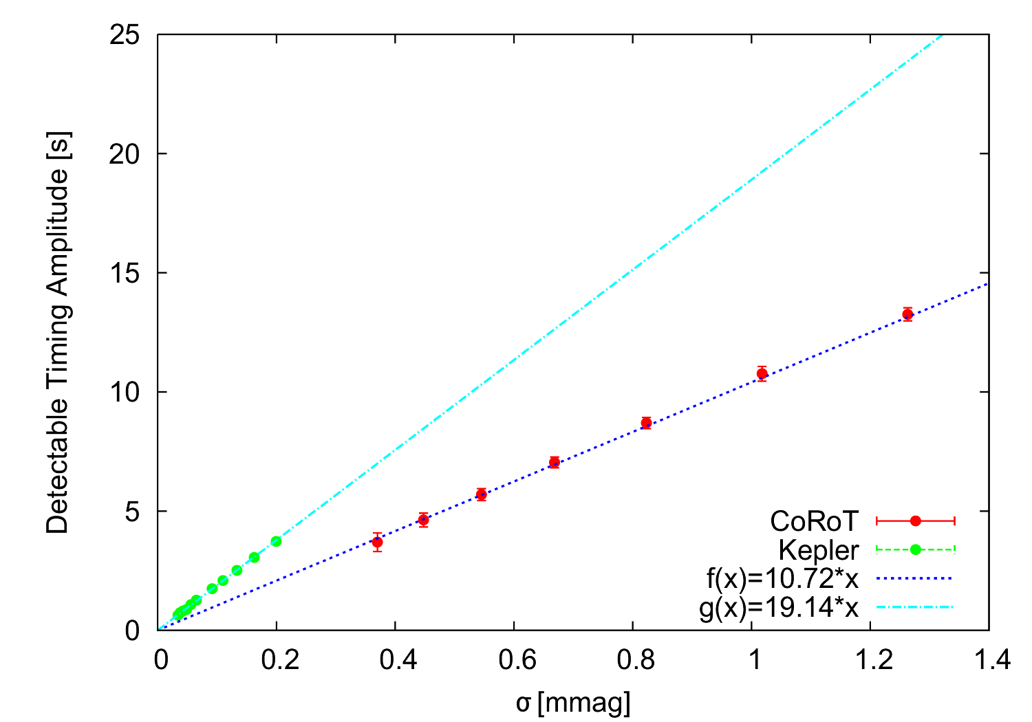
Figure 5: DTA for a given photometric precision for CoRoT and Kepler missions along with the best fitting relation. Note that the difference between the two cases is dependent on the cadence of photometric measuremenets (CoRoT $\sim$320 and Kepler $\sim$900 secodns).

The potential problem with both missions is the predefined target pool. If this is taken into account, despite high photometric precision the chances of detecting a circumbinary, non-transiting planet may be somewhat small. For example for the Kepler mission an upper limit to detectable circumbinary planets may be estimated as follows

$$n_{P}=n_{*}p_{*}p_{J}=10^{5}\cdot 0.00016\cdot 0.06=0.96$$ (6)

where:

• $n_{*}$ is the number of targets, $n_{*}\approx 10^{5}$ (kepler.nasa.gov),

• $p_{*}$ is the eclipsing detached binary stars ratio to all stars, $p_{*}\approx 0.00016$ (Paczyński et al., 2006),

• $p_{J}$ is the percentage of stars having giant planets (assuming that it is the same as for single stars), $p_{J}\approx 0.06$

and this does not take into account the probability of detecting a planet with a given mass and period via ET. Clearly, in order to detect circumbinary planets using ET one may have to turn to the ground based observations where the target pool can be carefully selected and fine-tuned to provide for the highest possible chances of detecting circumbinary planets. However, let us note that in the above we used a percentage of detached binaries in the ASAS catalogue. If one is willing to try the presumably less stable contact binaries as well, then $p_{*}$ increases to $\sim 0.00065$ according to the results from the ASAS sample (Paczyński et al., 2006). Even more optimistic preliminary results come from the Kepler and CoRoT fields for which the percentage of eclipsing binaries is $\sim 0.007$ (H. Deeg, L. Doyle personal communication). In such a case, the number of potentially detectable planets would rise to $\sim 40$.

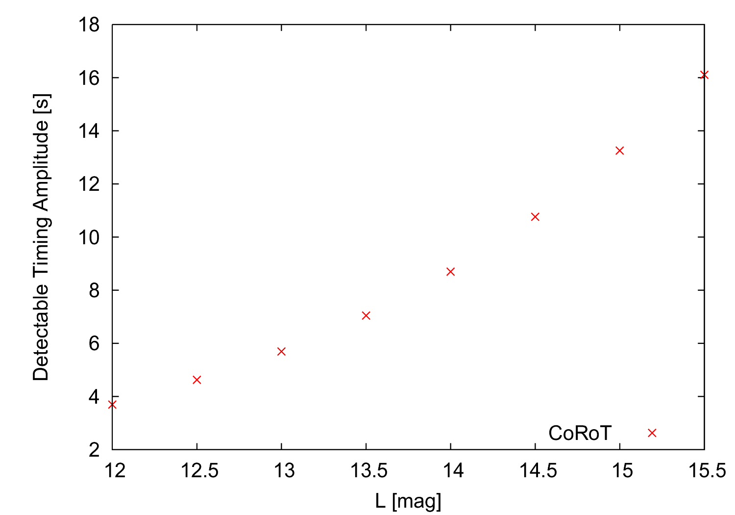
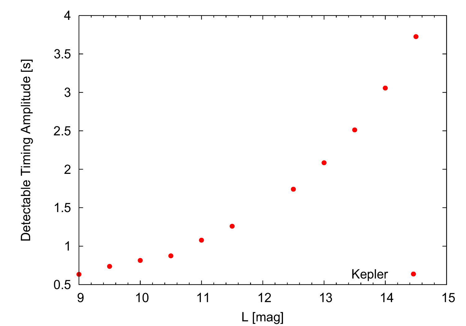
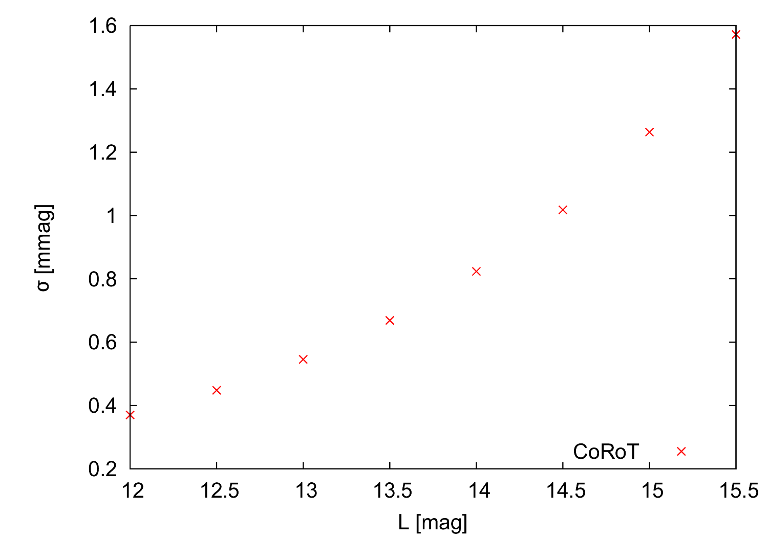
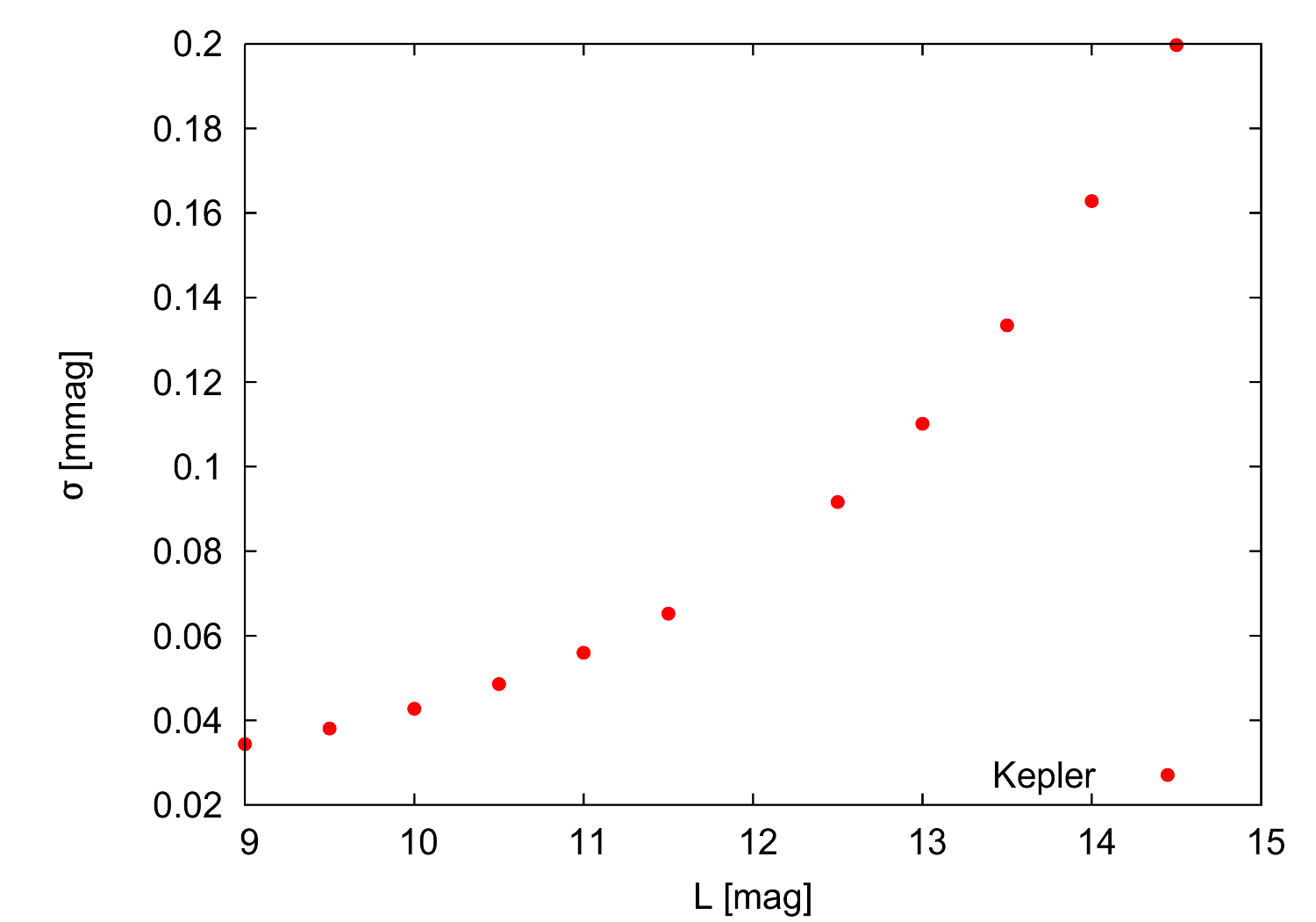
Figure 6: Typical DTA and photometric error for CoRoT (left) and Kepler (right) missions and an object with brightness $L$.

5 Observations from the ground

Performing numerical simulations that would aim to answer all or almost all questions related to a search for circumbinary planets using ground based ET is not practical. Possible observing scenarios are highly dependent on a choice of a target, its parameters and the coordinates of an observatory. Such simulations can be carried out if the target pool and the observatory are already chosen. For these reasons, we present below a few typical problems one may encounter when performing a ground based ET survey and analyze them through numerical simulations. These results are an essence of a much larger set of simulations we carried out.

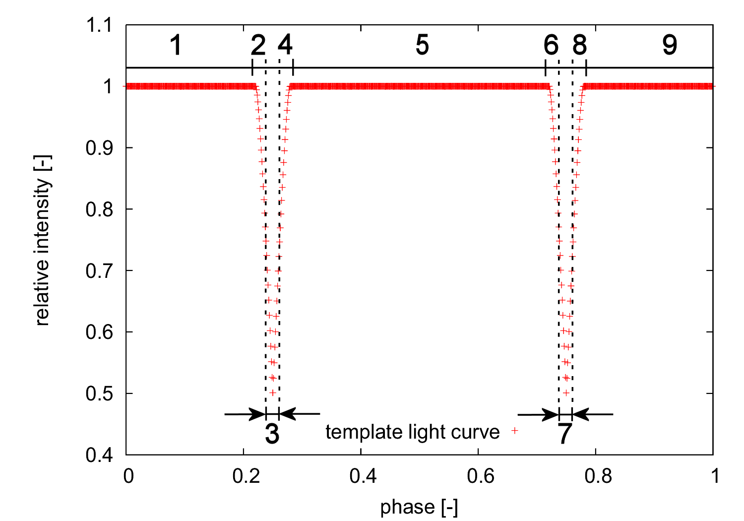
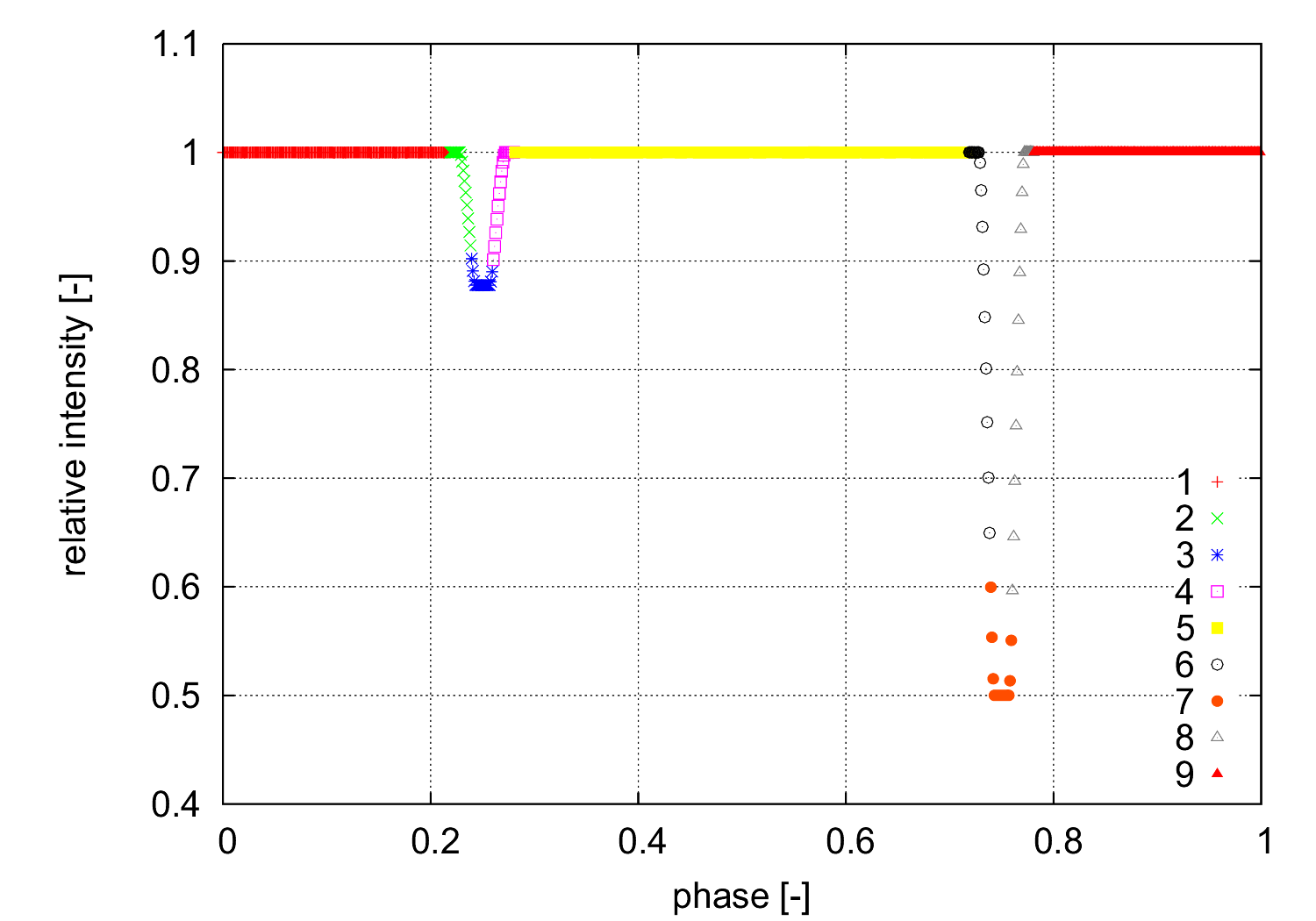
Figure 7: Light curve templates for simulations exploring an influence of the different parts of light curves on DTA. Figure 7 is the template of V-shape eclipses, 7 represents flat bottom eclipses.

Table 4: Impact of different parts of a light curve and their combinations on DTA (in seconds) for a V-shaped eclipse shown in Figure 7. DTA of 20 sec means that a timing measurement was not possible.

no. of active parts \ part no.	1	2	3	4	5	6	7	8	9
1	20.00	6.28	3.74	8.08	20.00	8.16	4.88	8.36	20.00
2	9.95	5.27	3.53	6.34	9.96	6.25	4.26	6.54	9.97
3	6.02	4.50	3.32	5.03	6.01	4.99	3.81	5.13	6.03
4	4.46	3.91	3.12	4.16	4.45	4.15	3.47	4.20	4.47
5	3.71	3.47	2.96	3.59	3.71	3.56	3.20	3.59	3.71
6	3.47	3.36	3.10	3.50	3.58	3.50	3.31	3.52	3.59
7	2.92	2.87	2.70	2.90	2.92	2.89	2.80	2.90	2.93
8	2.67	2.65	2.58	2.66	2.67	2.66	2.62	2.66	2.67
9	2.52	2.52	2.52	2.52	2.52	2.52	2.52	2.52	2.52

Table 5: Impact of different parts of a light curve and their combinations on DTA (in seconds) for an eclipse with a flat bottom shown in Figure 7. DTA of 20 sec means that a timing measurement was not possible.

no. of active parts \ part no.	1	2	3	4	5	6	7	8	9
1	20.00	6.88	20.00	20.00	20.00	4.29	9.60	4.21	20.00
2	12.89	6.76	11.33	11.46	14.51	3.80	8.10	3.87	12.89
3	8.52	6.75	7.61	7.58	9.52	3.52	5.43	3.65	8.51
4	5.14	4.87	5.14	4.85	5.15	3.29	4.51	3.39	5.17
5	4.77	4.49	4.56	4.53	4.72	3.16	3.91	3.22	4.72
6	3.54	3.48	3.51	3.52	3.54	2.93	3.36	3.00	3.53
7	3.06	3.04	3.05	3.06	3.06	2.78	3.00	2.82	3.06
8	2.76	2.75	2.75	2.75	2.75	2.65	2.74	2.66	2.76
9	2.55	2.55	2.55	2.55	2.55	2.55	2.55	2.55	2.55

The two main differences between the space and ground based surveys are the presence of red noise due to predominately the atmosphere and the typically very incomplete light curves one obtains with a ground based telescope for a detached eclipsing binary that typically has an orbital period much longer than the duration of a night. For our reference binary (Table 1), we simulated two types of light curves. One with V-shaped eclipses (the parameters exactly as in Table 1) and one with eclipses with flat bottoms. In the later case, we assumed a radius ratio of 0.5 while keeping $L_{2}=0.5$. To the simulated photometric measurements we added red noise with an RMS of 0.35 mmag, white noise with an RMS of 0.35 mmag and photon noise depended on the actual momentary brightness. We divided the light curves into 9 parts to explore which parts when present have the largest impact on the detectable timing amplitude (see Figures 7 and 7). In the simulations we removed parts of the light curves and used such incomplete light curves to measure the times of eclipse. All the possible permutations without repetition were used for sets ranging from 1 to 9 light curve’s elements. Afterwards an average DTA was calculated. Whenever a DTA could not be computed, the result by default was set to 20 sec. The results are shown in Tables 4, and 5. In the tables the columns correspond to the parts of light curve which were for sure present and the rows correspond to the total number of parts present (”active”) in a light curve. This approach allows us to easily determine the most valuable parts of a light curve and establish which sets of them when present provide even better results.

In the case of V-shaped eclipses the most important are the parts 3 and 7 in Figure 7 which correspond to the middle parts of eclipses. Next come ingress and egress. For the eclipses with flat bottoms the most valuable parts are 6 and 8 in Figure 7 (ingress and egress of the deeper eclipse). Altogether most of the timing information can be derive by just observing the entire eclipses. This is consistent with common sense and is doable from the ground. Let us also note that in the simulations we used the first type of red noise from Figure 3. We also determined that its impact on the detectable timing amplitude is comparable to white noise with and RMS twice as large (i.e. 0.7 mmag).

In another set of simulations we tested a number of features of an eclipse that affect the timing precision and detectable amplitude. We tested the impact of the duration of a flat part of an eclipse (Figure 8), the impact of the eclipse’s depth (Figure 9), the impact of the duration of a V-shaped eclipse, the impact of the secondary star’s luminosity (Figure 11) and the radius ratio (Figure 12) on the detectable timing amplitude (DTA). The conclusion is that it is preferable to observe V-shaped short lasting and deep eclipses to maximize DTA which is not an unexpected result.

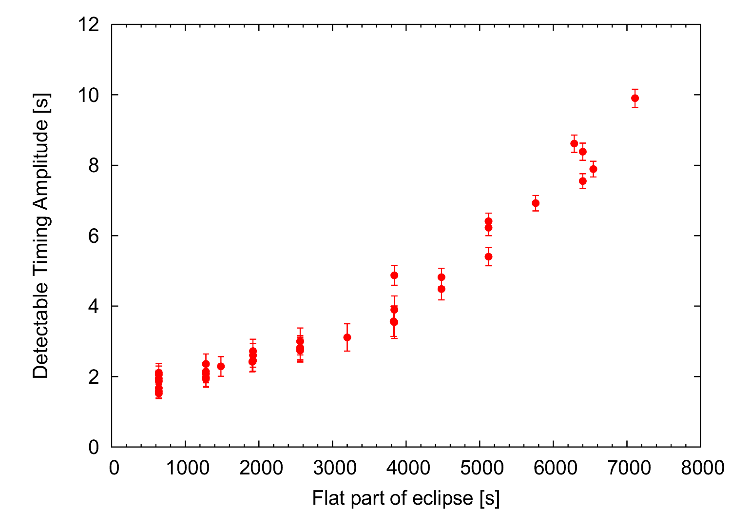
Figure 8: Duration of the flat part of an eclipse and DTA.

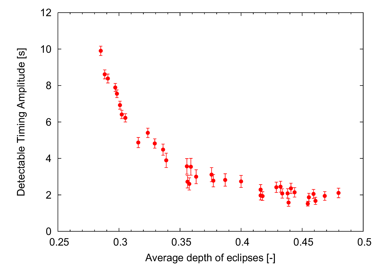
Figure 9: Depth of an eclipse and DTA.

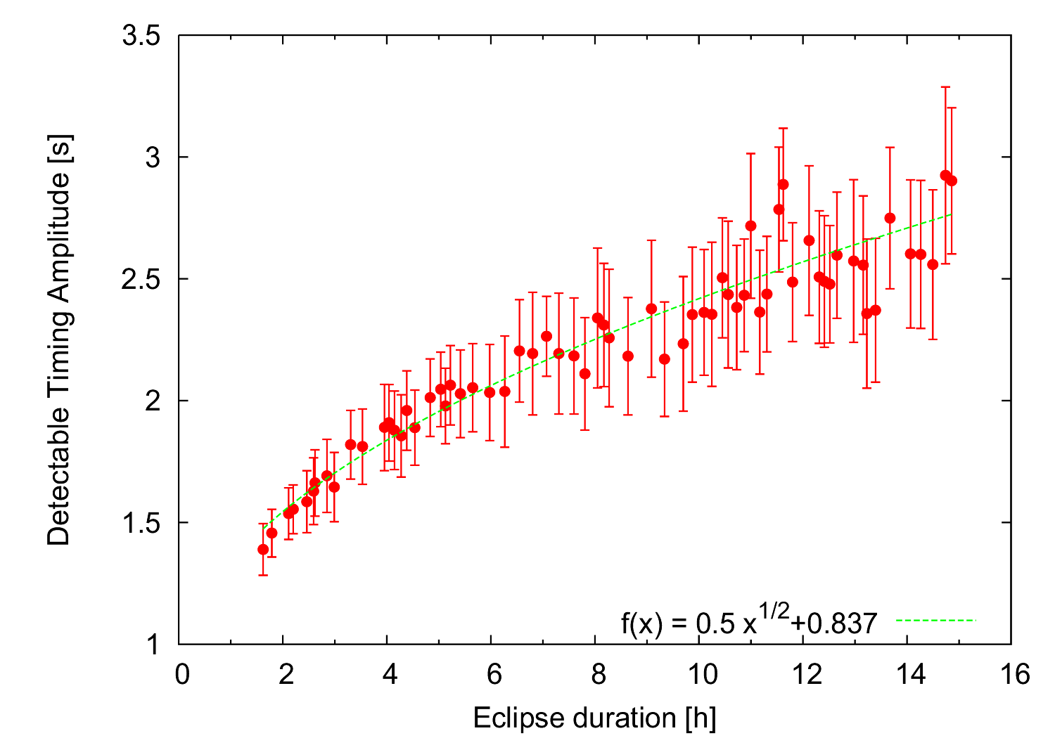
Figure 10: Duration of an eclipse and DTA. The solid line represents the analytic approximation by Doyle & Deeg 2004.

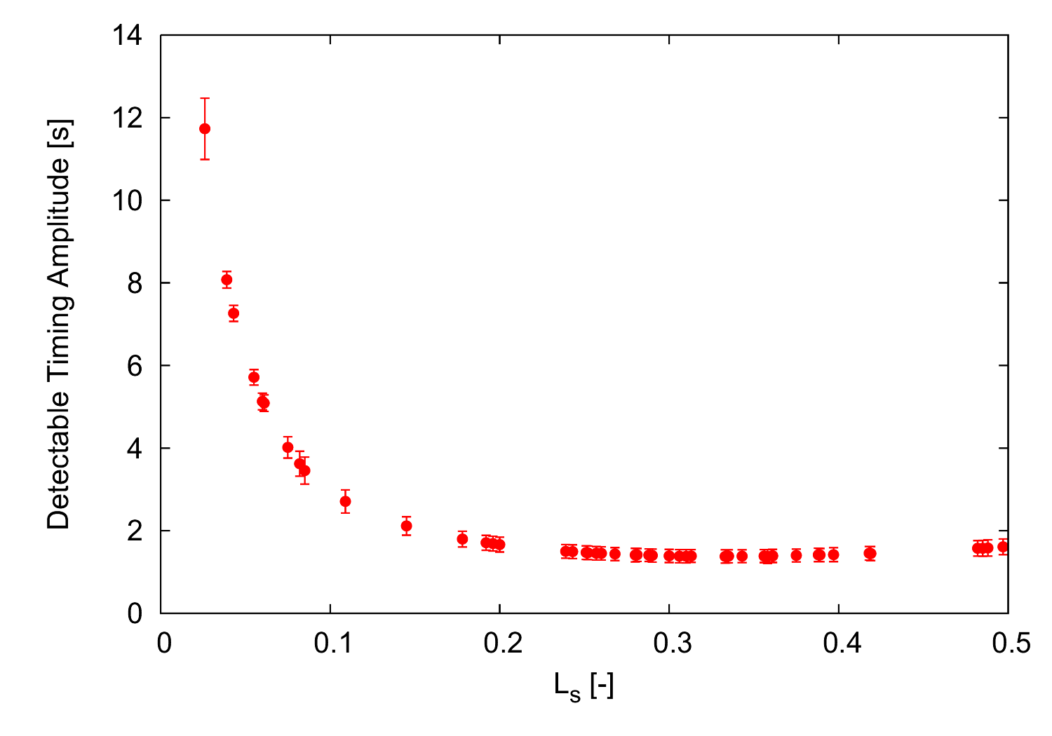
Figure 11: Impact of the second star’s luminosity $L_{S}$ in units of the primary star’s luminosity on the detectable timing amplitude.

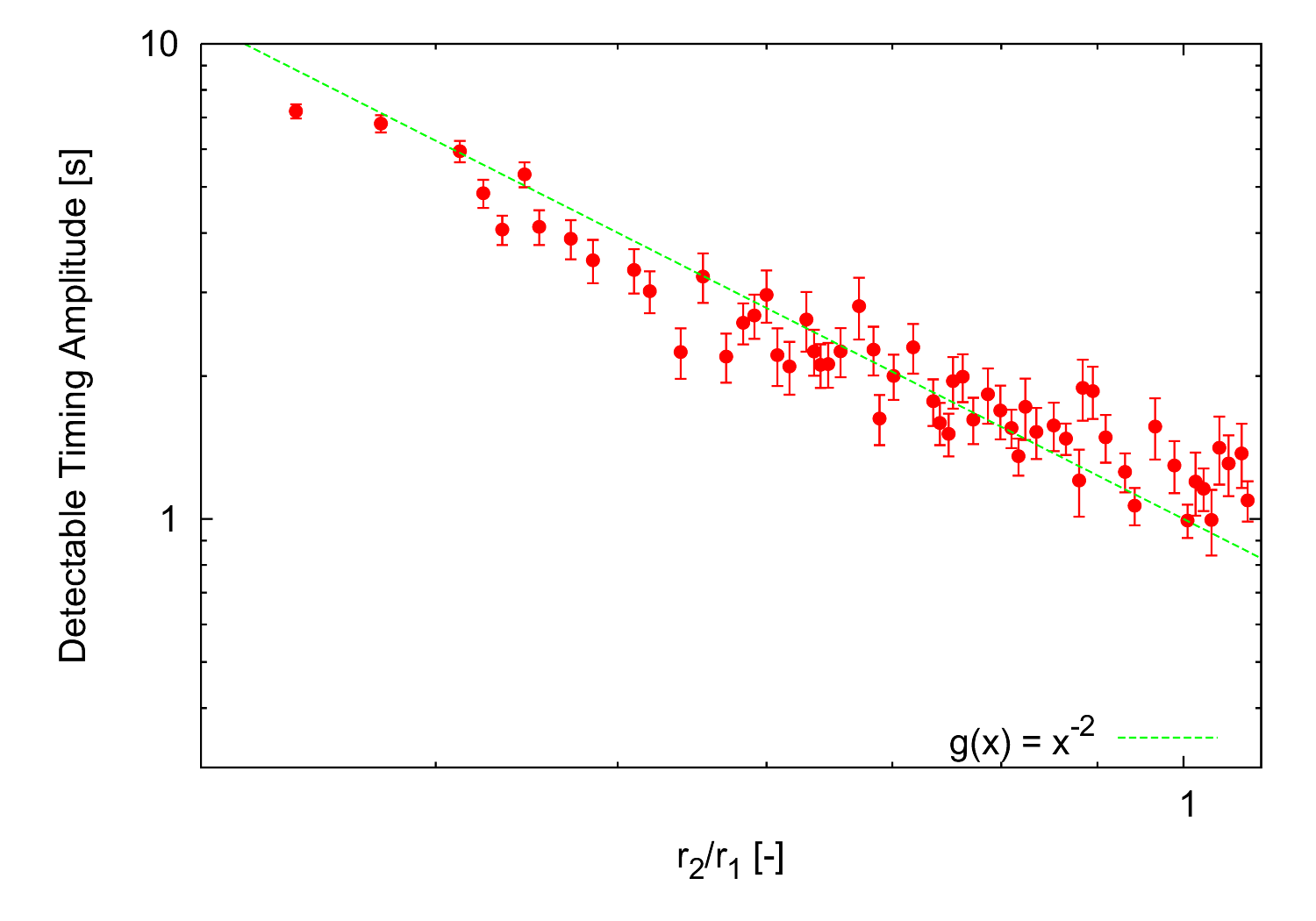
Figure 12: Detectable timing amplitude as a function of the ratio of radii of the secondary and primary star ($r_{2}/r_{1}$). In these simulations the parameters for the ground based case were used.

Let us note that Doyle & Deeg (2004) derived an equation allowing one to estimate an eclipse timing precision assuming that the eclipse has a simple triangular shape

$$\delta_{t_{0}}\approx\delta_{L}\frac{T_{ec}}{2\Delta L\sqrt{N}}$$ (7)

where $T_{ec}$ is the duration of an eclipse, $N$ is the number of photometric measurements taken during $T_{ec}$ and $\Delta L$ is the relative depth of the eclipse. Our simulations prove that this is a good approximation. This can be seen in Figure 10 where one should note that after introducing the integration time $T_{int}$, we have $N=T_{ec}/T_{int}$ and the equation 7 can be rewritten as

$$\delta_{t_{0}}\approx\delta_{L}\frac{\sqrt{T_{ec}T_{int}}}{2\Delta L}$$ (8)

In the above, $T_{int}$ is constant, the DTA is approximately equal to $\delta_{t_{0}}$ and the square root relation between $\delta_{t_{0}}$ and $T_{ec}$ is visible.

We conclude the simulations with two representative figures for a ground base survey based on a 0.5-m telescope. Figure 13 shows DTA and Figure 14 a typical photometric error due to the photon noise for our test scenario.

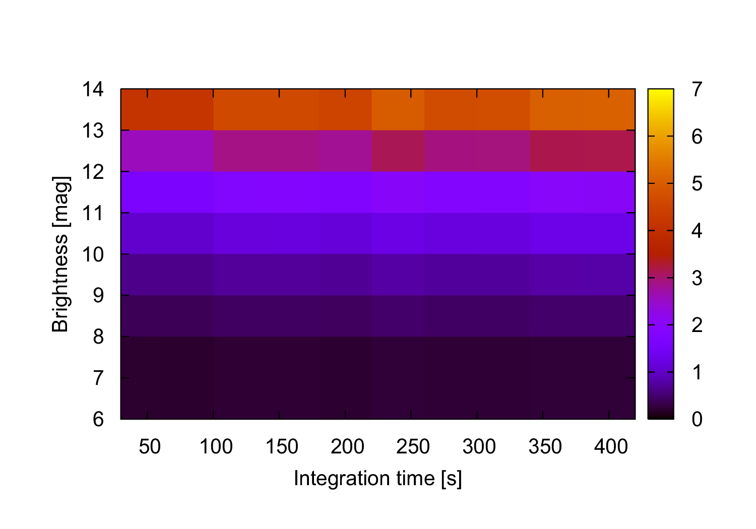
Figure 13: DTA as a function of the integration time and brightness of the target for a ground-based effort.

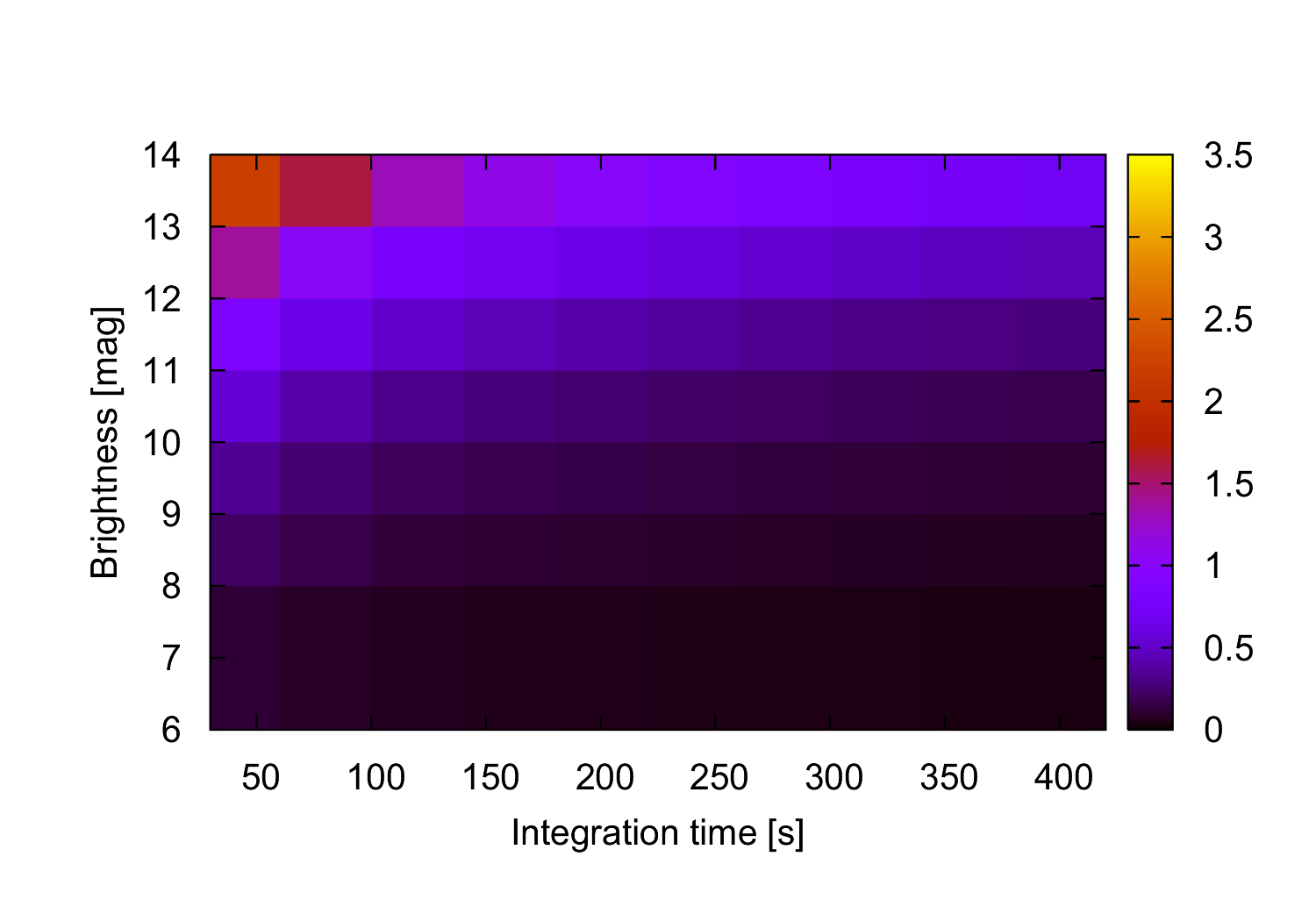
Figure 14: Photometric precision in mmag as a function of the integration time and brightness of the target for a ground-based effort.

6 Conclusions

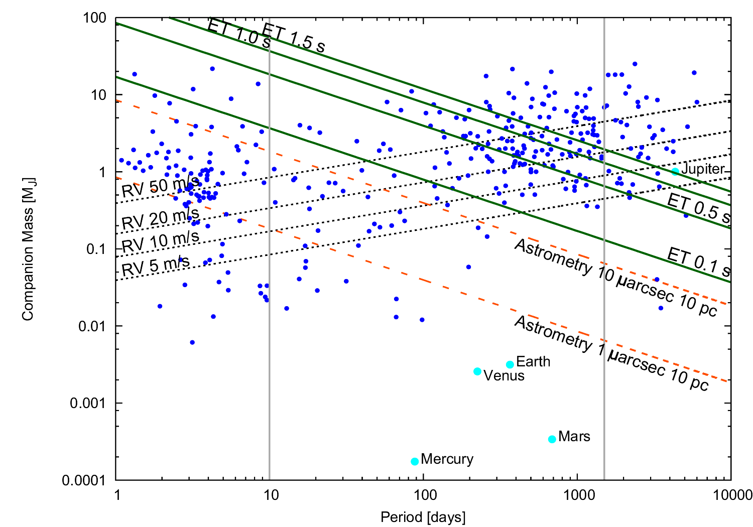
Figure 15: Discovery space for circumbinary planets around a binary star composed of two Sun-like stars. Known exoplanets are marked with dots. The two vertical lines correspond to the shortest stable orbit for this case (Dvorak, 1989; Holman & Wiegert, 1999) and 4 years.

In order to detect giant circumbinary planets around eclipsing stars a timing precision of the order of 0.1-1 seconds is necessary. The Kepler and CoRoT missions are capable of providing photometric precision sufficient to reach such a timing precision. However, in both cases what makes the detections challenging is a predefined target pool. In the case of CoRoT typical targets are quite faint and the duration of an observing window is only 150 days which effectively limits the detection capabilities to brown dwarfs. In the case of Kepler, the target pool puts an upper limit of potentially detectable circumbinary gas giants at about 40 in the best case scenario. This number does not take into account the orbital and physical parameters of circumbinary planets (like e.g. masses). Hence, the more realistic upper limit is expected to be up to several times lower. Nevertheless, both missions still may deliver us a detection of a circumbinary planet via eclipse timing. It seems that the best strategy to detect circumbinary planets around eclipsing binary stars is by carrying out a ground based survey for which targets can be carefully preselected. Such survey would have to employ several 0.5-m class telescopes to be efficient. As the survey would typically focus on the shorter period detached eclipsing binary stars (see Figure 10), it would target a different set of targets than a radial velocity based survey.

In Figure 15 we compare planet detection capabilities of the radial velocity, astrometry and eclipse timing. Eclipse timing which is essentially a 1-d astrometric measurement is complementary to the radial velocity technique and as we have demonstrated one is able to achieve a timing precision sufficient to detect giant planets. Finally, let us note that two circumbinary planets around an eclipsing binary HW Vir (Lee et al., 2009), a circumbinary brown dwarf around an eclipsing binary HS0705+6700 (Qian et al., 2009) and a giant planet around an eclipsing polar DP Leo (Qian et al., 2010) were claimed to be detected by means of eclipse timing. However, it is hard to judge if these cases of timing variation are really caused by substellar companions and not an unknown quasi-periodic phenomenon. Nevertheless this is yet another proof that eclipse timing is becoming a useful tool for detecting subtle timing variations.

References

- Alonso et al. (2008) Alonso R., Auvergne M., Baglin A., Ollivier M., Moutou C., Rouan D., Deeg H. J., Aigrain S. et al., 2008, A&A, 482, L21
- Auvergne et al. (2009) Auvergne M., Bodin P., Boisnard L., Buey J. -T., Chaintreuil S., Epstein G., Jouret M., Lam-Trong T. et al., 2009, A&A, 506, 411
- Costes et al. (2004) Costes V., Bodin P., Levacher P., Auvergne M., 2004, 5th International Conference on Space Optics, 554, 281
- Cumming (2004) Cumming A., 2004, MNRAS, 354, 1165
- Deeg et al. (2008) Deeg H. J., Ocaña B., Kozhevnikov V. P., Charbonneau D., O’Donovan F. T., Doyle L. R., 2008, A&A, 480, 563
- Doyle & Deeg (2004) Doyle L. R., Deeg H. J., 2004, Bioastronomy 2002: Life Among the Stars, 213, 80
- Dvorak (1984) Dvorak R., 1984, Celestial Mechanics, 34, 369
- Dvorak (1989) Dvorak R., Froeschle C., Froeschle C., 1989, A&A, 226, 335
- Garrido & Deeg (2006) Garrido R., Deeg H. J., 2006, Lecture Notes and Essays in Astrophysics, 2, 27
- Holman & Wiegert (1999) Holman M. J., Wiegert P. A., 1999, AJ, 117, 621
- Koch et al. (2004) Koch D. G., Borucki W., Dunham E., Geary J., Gilliland R., Jenkins J., Latham D., Bachtell E. et al., 2004, Proc. SPIE, 5487, 1491
- Lee et al. (2009) Lee J. W., Kim S.-L., Kim C.-H., Koch R. H., Lee C.-U., Kim H.-I., Park J.-H., 2009, AJ, 137, 3181
- Milotti (2006) Milotti E., 2006, Computer Physics Communications, 175, 212
- Milotti (2007) Milotti E., 2007, Phys. Rev, 75, 011120
- Moré et al. (1980) Moré J. J., Garbow B. S., Hillstrom K. E., 1980, User Guide for MINPACK-1, Argonne National Laboratory Report ANL-80-74
- Moré et al. (1984) Moré J. J., Sorensen D. C., Hillstrom K. E., Garbow, B. S., 1984, The MINPACK Project, in Sources and Development of Mathematical Software, W. J. Cowell, ed., 88-111
- Muterspaugh et al. (2007) Muterspaugh M. W., Konacki M., Lane B. F., Pfahl E., 2007, preprint (arXiv:astro-ph/0705.3072v1)
- Nelson & Davis (1972) Nelson B., Davis W. D., 1972, ApJ, 174, 617
- Ofir et al. (2009) Ofir A., Deeg H. J., Lacy C. H. S., 2009, A&A, 506, 445
- Paczyński et al. (2006) Paczyński B., Szczygieł D. M., Pilecki B., Pojmański G., 2006, MNRAS, 368, 1311
- Qian et al. (2010) Qian S.-B., Liao W.-P., Zhu L.-Y., Dai Z.-B., 2010, ApJ, 708, L66
- Qian et al. (2009) Qian S.-B., Dai Z.-B., Liao W.-P., Zhu L.-Y., Liu L., Zhao E. G., 2009, ApJ, 706, L96