Sensitivity analysis of random two-body interactions

Abstract

The input to the configuration-interaction shell model includes many dozens or hundreds of independent two-body matrix elements. Previous studies have shown that when fitting to experimental low-lying spectra, the greatest sensitivity is to only a few linear combinations of matrix elements. Here we consider interactions drawn from the two-body random ensemble, or TBRE, and find that the low-lying spectra are also most sensitive to only a few linear combinations of two-body matrix elements, in a fashion nearly indistinguishable from an interaction empirically fit to data. We find in particular the spectra for both the random and empirical interactions are sensitive to similar matrix elements, which we analyze using monopole and contact interactions.

I Introduction and Motivation

The configuration-interaction shell model is a useful framework for a detailed understanding of low-energy nuclear structure BG77 ; br88 ; ca05 . The many-body basis is a large dimension ($10^{3-10}$) set of Slater determinants, which are antisymmeterized products of single-particle states. One must truncate the single-particle states, corresponding to one or a few shells (typically using the harmonic oscillator as an approximation to the mean-field); the many-body basis may be further truncated. For phenomenological calculations one writes the Hamiltonian in terms of single-particle energies and two-body matrix elements, while for ab initio calculations one may extend this to three-body interactions NO03 .

The two-body matrix elements are the matrix elements of the residual interaction in the lab frame,

$$V_{JT}(ij,kl)=\langle ij;JT|\hat{V}|kl;JT\rangle$$ (1)

where $|ij;JT\rangle$ is the normalized, antisymmeterized product of particles in orbits labeled by $i$ and $j$ and coupled to good angular momentum $J$ and isospin $T$. If one starts from a translationally invariant interaction between particles, one can either compute the integral in the lab frame or start in the relative frame and then transform to the lab frame; in either case there are correlations between the matrix elements, although they are not obvious to the casual observer.

Often for semi-phenomenological calculations, one starts from a “realistic” interaction, and then adjusts the two-body matrix elements until the rms error on a set of experimentally known energy levels is minimized BG77 . In the $1s$-$0d$ shell, such a semi-phenomenological interaction has been recently derived br06 , improving on an earlier interactionWildenthal .

It has been found that the fits are empirically dominated by a few linear combinations of matrix elements. The physical meaning of those dominant combinations is not immediately obvious. One might naively guess the linear correlations are due to an underlying translationally invariant interaction (although a density dependence would destroy this). Somewhat more phenomenologically, it has been argued by appealing to mean-field properties that one can improve fits primarily through adjusting the monopole-monopole part of the interaction, that is, interaction terms that look like $n_{a}(n_{b}-\delta_{ab})$, where $n_{a}$ is the number of particles in the $a$th orbit. This protocol for shifting monopole strengths has been successfully applied to several semi-empirical interactions po81 ; ma97 ; ut99 ; ho04 ; su06

A related study BJ09 , investigating the origin of many-body forces from truncation of the model space, also found an empirical fit dominated by a few linear combinations of matrix elements. While much of the fit was dominated by the monopole interactions, even better agreement was brought about using a contact interaction motivated by its usage in mean-field calculations sk56 ; be03 and effective field theoryvk99 .

In investigating the character and origin of the dominant matrix elements, it is useful to ask if there is anything special about the nuclear interaction. One way to ask this question is to compare with interactions drawn from the two-body random ensemble (TBRE), which despite their arbitrary nature are known to echo some features of real nuclear spectra JBD98 ; ZV04 ; ZAY04 ; PW07 . In this paper we conduct a sensitivity analysis of the low-lying spectra of random interactions and compare against a standard empirical interaction, USDB. We find that for more measures all the interactions are nearly indistinguishable, at least on a statistical level.

II Methodology and results

Our methodology follows previous work BG77 ; br06 ; BJ09 ; we work in the $1s$-$0d$ valence space with an inert ¹⁶O core. Given an input set of two-body matrix elements (we leave aside single-particle energies and any $A$-dependent scaling), which we write as a vector $\vec{v}$, we can calculate the eigenvalues $E_{\alpha}(\vec{v})$ of the many-body Hamiltonian. For this work the label $\alpha$ ranged over all nuclides with $0\leq Z_{\mathrm{valence}}\leq N_{\mathrm{valence}}\leq 10$ and took the ground state binding energy and the first five excitation energies.

If one has a target spectrum $E_{\alpha}^{0}$, say from experiment, then the goal of the fit is to minimize

$$\sum_{\alpha}\left(E_{\alpha}(\vec{v})-E_{\alpha}^{0}\right)^{2}$$ (2)

(for simplicity we leave off the experimental uncertainty in each state). Expanding to first order

$$E_{\alpha}(\vec{v}+\delta\vec{v})\approx E_{\alpha}(\vec{v})+\sum_{i}\delta v_{i}\frac{\partial E_{\alpha}}{\partial v_{i}}$$ (3)

then minimizing (2) yields

$$\sum_{\alpha}\left(E_{\alpha}(\vec{v})-E_{\alpha}^{0}\right)\frac{\partial E_{\alpha}}{\partial v_{i}}=\sum_{j}\sum_{\alpha}\frac{\partial E_{\alpha}}{\partial v_{i}}\frac{\partial E_{\alpha}}{\partial v_{j}}\delta v_{j}.$$ (4)

This equation is in the form $\vec{b}=\mathbf{A}\vec{x}$ where

$$A_{ij}=\sum_{\alpha}\frac{\partial E_{\alpha}}{\partial v_{i}}\frac{\partial E_{\alpha}}{\partial v_{j}}.$$ (5)

The derivatives come via the Hellmann-Feynman theorem F39

$$\frac{\partial E_{\alpha}}{\partial v_{i}}=\left\langle\Psi_{\alpha}\left|\hat{H}_{i}\right|\Psi_{\alpha}\right\rangle$$ (6)

where $\hat{H}_{i}$ is the Hamitonian operator whose strength is $v_{i}$.

We then find the eigenvalues of $\mathbf{A}$ (which is equivalent to finding the squares of the eigenvalues in the singular-value decomposition of $\partial E_{\alpha}/\partial v_{i}$). We do this for both the USDB interaction and for an ensemble of 100 sets of random two-body interactions, also called the two-body random ensemble (TBRE). The results are shown for the TBRE in Fig. 1, where we have separated out the sensitivity just for the binding energies (ground state energies) and the excitation energies. Although not shown, the equivalent SVD eigenvalues for USDB are completely within the TBRE results.

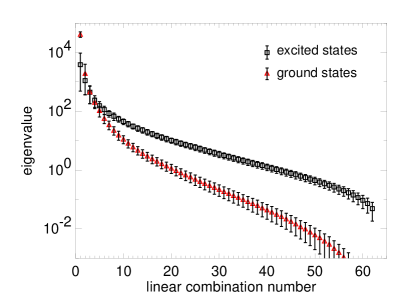
Figure 1: (Color online)The spectra of eigenvalues from a singular-value decomposition of the sensitivity matrix $\mathbf{A}$ (Eq. 5) for the two-body random ensemble. The lower curve is for ground state energies, while the upper curve is for excitation energies.

The lower curve is for ground states only, while the upper curve is for excitations energies relative to the ground state. Clearly, and perhaps unsurprisingly, the ground state energies are predominantly sensitive to just a few linear combinations of matrix elements–significantly fewer than excitations energies.

Fig. 1 characterizes eigenvalues of $\mathbf{A}$. The next step is to characterize the eigenvectors associated with the dominant eigenvalues, specifically by comparing with monopole and contact interactions. To do so we first discuss a method for quantifying the overlap between two vector subspaces MC ; SK08 . Consider two vectors subspaces, $S_{1}$ and $S_{2}$. Let $\mathbf{V}_{1}$ be a matrix whose column vectors are the (orthonormal) basis vectors of $S_{1}$, and similarly with $\mathbf{V}_{2}$. From these one constructs the overlap matrix $\mathbf{\Omega}=\mathbf{V}_{1}^{\dagger}\mathbf{V}_{2}$. Note that if the subspaces are not of equal dimension then $\mathbf{\Omega}$ is not a square matrix. In any case we do a singular value decomposition of $\mathbf{\Omega}$; the SVD eigenvalue spectrum then is a measure of the overlap of the two spaces. If the two spaces perfectly overlap then all eigenvalues are 1, if just $N$ of the dimensions perfectly overlap than $N$ eigenvalues will be 1 and the rest zero. Note that this method is invariant under arbitrary choice of orthonormal bases.

We begin with the monopole-monopole interaction of the form $n_{a}(n_{b}-\delta_{ab})$, which has six unique terms, and thus six vectors or linear combinations of matrix elements, in the $sd$-shell. These we combine with the $k$ most dominant linear combinations that arise from the previous analysis; somewhat arbitrarily we chose $k=6$ (our results do not change qualitatively for other small values of $k$). The results, the SVD eigenvalues of $\Omega$, are shown in Fig. 2. It is important to note we compute the spectrum separately for each randomly generated interaction and then compute the distribution.

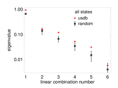
Figure 2: (Color online) The SVD spectrum that measures the overlap of the subspace defined by the six largest eigenvectors from Fig. 1, with the subspace defined by the monopole-monopole interaction. (Black) squares are for the TBRE, while (red) diamonds are for USDB.

The results for ground states and for excited states are similar, so we combine all states into a single calculation. The eigenvalues for USDB are roughly $50\%$ higher than for the TBRE, but otherwise qualitatively very similar.

We also compared for contact interactions; we took only two terms, the $S=0,T=1$ channel and $S=1,T=0$ channel (there being only the $s$-wave channel in relative coordinates). These results we summarize in Table 1.

Table 1: Leading eigenvalues from SVD of subspace overlaps of two-term contact interaction

Interaction	ground states	excited states	all states
USDB	0.60	0.58	0.62
TBRE	$0.55\pm 0.04$	$0.41\pm 0.06$	$0.55\pm 0.04$

For comparison, the leading eigenvalue for the overlaps of USDB versus the six-term monopole is 0.94, while that of the TBRE versus monopole is $0.66\pm 0.03$. There is somewhat more sensitivity to the monopole interaction than the contact interaction; however, the reader should keep in mind that is not the whole story. Recall that when fitting an interaction, the linearized equations are cast in the form $\mathbf{A}\vec{x}=\vec{B}$. Our analysis in this paper is entirely with the eigenvalues of $\mathbf{A}$, but in any fit one must also look to $\vec{b}$ (which in practice is the deviation of the theoretical spectra from experiment). For example, in BJ09 it was found that using a contact interaction brought better agreement than a monopole interaction. One can understand this in terms of conjugate gradient methods NR : the direction of local steepest gradient may not in fact point towards the global minimum.

Figure 3: SVD spectrum from the overlap of the dominant eigenvectors from USDB and the TBRE.

By our measures so far, both the TBRE and the empirically-fit USDB look qualitatively similar. Therefore we take a final analysis by comparing the dominant linear combinations of the USDB with those from the TBRE. This is show in Fig. 3, using the same analysis as for Fig. 2. For comparison with the previous results, the leading eigenvalue is $0.72\pm 0.06$.

III Conclusion

We have analyzed the sensitivity of the low-lying spectra of the random two-body ensemble of interactions to variations of the Hamiltonian matrix elements; by using singular value decomposition, we find the dominant linear combinations, which would be important in any fit to experimental data. We found the SVD eigenvalues follow a pattern remarkably similar to that shown by semi-realistic/semi-phenomenological interactions such as USDB. We also analyzed the most dominant linear combinations of matrix elements by computing the overlap with monopole and contact interactions. Overall, both the TBRE and the empirical USDB had qualitatively similar results.

The U.S. Department of Energy supported this investigation through contracts DE-FG02-96ER40985 and DE-FC02-09ER41587, and through subcontract B576152 by Lawrence Livermore National Laboratory under contract DE-AC52-07NA27344.

References

- (1) P.J. Brussard and P.W.M. Glaudemans, Shell-model applications in nuclear spectroscopy (North-Holland Publishing Company, Amsterdam, 1977).
- (2) B. A. Brown and B. H. Wildenthal, Annu. Rev. Nucl. Part. Sci. 38, 29 (1988).
- (3) E. Caurier, G. Martínez-Pinedo, F. Nowacki, A. Poves, and A. P. Zuker, Rev. Mod. Phys. 77, 427 (2005).
- (4) P. Navrátil and W. E. Ormand, Phys. Rev. C 68, 034305 (2003).
- (5) B.A. Brown and W.A. Richter, Phys. Rev. C 74 034315 (2006).
- (6) B.H. Wildenthal, Prog. Part. Nucl. Phys. 11, 5 (1984).
- (7) A. Poves and A. Zuker: Phys. Rep. 70, 235 (1981).
- (8) G. Martínez-Pinedo, A. P. Zuker, A. Poves, and E. Caurier, Phys. Rev. C55 187 (1997).
- (9) Y. Utsuno, T. Otsuka, T. Mizusaki, and M. Honma: Phys. Rev. C 60, 054315 (1999).
- (10) M. Honma, T. Otsuka, B. A. Brown, and T. Mizusaki, Phys. Rev. C 69, 034335 (2004).
- (11) T. Suzuki, S. Chiba, T. Yoshida, T. Kajino, and T. Otsuka Phys.Rev. C 74, 034307 (2006).
- (12) G. F. Bertsch and C. W. Johnson, Phys. Rev. C 80, 027302 (2009).
- (13) T.H.R. Skyrme, Philos. Mag. 1, 1043 (1956).
- (14) M. Bender, P.-H. Heenen, and P.-G. Reinhard, Rev. Mod. Phys. 75, 121 (2003)
- (15) U. van Kolck, Prog. Part. Nucl. Phys. 43, 337 (1999); P. F. Bedaque and U. van Kolck, Annu. Rev. Nucl. Part. Sci. 52, 339 (2002); E. Epelbaum, Prog. Part. Nucl. Phys. 57, 654 (2006).
- (16) C. W. Johnson, G. F. Bertsch, and D. J. Dean Phys. Rev. Lett. 80, 2749 (1998).
- (17) V. Zelevinsky and A. Volya, Phys. Rep. 391, 311 (2004).
- (18) Y. M. Zhao, A. Arima, and N. Yoshinaga, Phys. Rep. 400, 1 (2004).
- (19) T. Papenbrock and H. A. Weidenmüller, Rev. Mod. Phys. 79, 997 (2007)
- (20) H. Hellman, Einführung in die Quantenchemie (Franz Deuticke, Leipzig, 1937), p. 285; R. P. Feynman, Phys. Rev. 56, 340, (1939).
- (21) G. H. Golub and C. F. van Loan, Matrix Computations, Second Edition (The Johns Hopkins University Press, Baltimore, 1989)
- (22) S. Kvaal, Phys. Rev. C 78, 044330 (2008).
- (23) W. H. Press, S. A. Teukolsky, W. T. Vetterling, and Brian P. Flannery, Numerical Recipes in Fortran, Second Edition (Cambridge University Press, Cambridge, 1992).