Imaging Redshift Estimates for BL Lacertae Objects

Abstract

We have obtained high dynamic range, good natural seeing $i^{\prime}$ images of BL Lacertae objects (BL Lacs) to search for the AGN host and thus constrain the source redshift. These objects are drawn from a sample of bright flat-spectrum radio sources that are either known (via recent Fermi LAT observations) gamma-ray emitters or similar sources that might be detected in continuing gamma-ray observations. All had spectroscopic confirmation as BL Lac sources, but no redshift solution. We detected hosts for 25/49 objects. As these galaxies have been argued to be standard candles, our measured host magnitudes provide redshift estimates (ranging from 0.2–1.0). Lower bounds are established on the redshifts of non-detections. The mean of the fit redshifts (and lower limits) is higher than those of spectroscopic solutions in the radio- and gamma-ray- loud parent samples, suggesting corrections may be needed for the luminosity function and evolution of these sources.

1. Introduction

BL Lac objects, being highly continuum-dominated, are a perennial problem for those wishing to study the evolution of AGN populations. The lack of visible broad lines and, even more, the low equivalent width of host absorption features makes redshift determinations extraordinarily difficult. Yet, since the continuum domination is a manifestation of the good alignment of the relativistic jet outflow to the Earth line-of-sight, (Urry & Padovani, 1995) knowledge of the distance, and hence luminosity scale, of these sources is very interesting.

This problem has become particularly important with gamma-ray detection of large numbers of blazars with the Fermi LAT (Abdo et al., 2009b). It has been known since EGRET that radio loud flat spectrum blazars dominate the bright extragalactic sources in the GeV sky (Hartmann et al., 1999; Mattox et al., 2001; Sowards-Emmerd et al., 2005); these objects are flat-spectrum radio quasars (FSRQ) and radio loud BL Lacs. We have good techniques in place to identify likely radio counterparts for the gamma-ray sources. Extensive spectroscopy campaigns, especially on the EGRET-like ‘CGRaBS’ sample (Healey et al., 2008) have provided nearly complete redshifts and characterizations of the FSRQ. However, despite extensive observation, including 8+m telescope integrations, less than half of the BL Lac counterparts have spectroscopic IDs. In some cases, high quality spectroscopy can give useful lower limits on the source redshift (Shaw et al., 2009), but many remain unconstrained. In the first LAT blazar catalog (Abdo et al., 2009a), the problem is even more pronounced since the excellent high energy response of the LAT favors detection of hard spectrum sources. BL Lacs are substantially harder ($\langle\Gamma\rangle\approx 2.0$) than FSRQ ($\langle\Gamma\rangle\approx 2.4$) and so provide a larger fraction, $\sim 40$% of the Fermi blazar sample, than was seen by EGRET.

We attempt here to constrain the redshifts of radio loud BL Lacs which have shown no convincing spectroscopic redshift solution, despite sensitive observations on large telescopes, by high dynamic range imaging searches for the AGN host. Our targets are drawn from the ‘CRATES’ catalog of bright flat-spectrum $|b|>10^{\circ}$ radio sources (Healey et al., 2007). Specifically, in this program we targeted the subset of CRATES consisting of $i$) sources selected as likely gamma-ray blazars before the Fermi mission (i.e. CGRaBS sources, Healey et al. 2008) and $ii$) sources that are likely counterparts to LAT sources detected early in the mission (Abdo et al., 2009a, 2010). All sources are at Declination $>-20^{\circ}$ and all have been shown to display featureless optical spectra (Healey et al., 2008; Shaw et al., 2009, 2010), with sensitive (4m+ class) observations. We were able to image $\sim 2/3$ of the sources satisfying these critera at the time of the observing campaigns.

It has been claimed (Sbarufatti et al., 2005) that BL Lac host galaxies detected with HST imaging are remarkably uniform giant ellipticals with $M_{R}=-22.9$; accordingly host detections can give redshift estimates and upper limits on the host flux can give lower limits on the distance. Here we do not test this assumption or the possible biases that would select a modest magnitude range for the detected host sample. We simply apply the method to extract redshift constraints, noting that while individual redshifts are doubtless imprecise, the estimates can still be useful for statistical studies of BL Lac evolution and as a guide to and comparison with other methods of redshift estimation. Conversely, when precision spectroscopic redshifts become available, our measurements can be used to help constrain the host evolution.

Since we will be searching for de Vaucouleurs profile excesses in the wings of the stellar PSF of the bright BL Lac core, we require good natural seeing and a moderate field of view for adequate comparison stars. For example, while near-IR adaptive optics can deliver superior PSF cores, the wings of the source at $>$90% encircled energy are extensive and often quite variable over the small corrected FoV. This prevents the accurate PSF modeling and subtraction required to obtain host measurements whose integrated magnitude can be 10% or less of the core flux.

2. Observations & Data Reduction

All observations were carried out using the WIYN 3.6m telescope at Kitt Peak National Observatory, which features good natural seeing and a $\sim 10^{\prime}$ FoV with the standard mosaic imagers.

2.1. OPTIC Camera

We employed OPTIC on the nights of 2008 Oct. 31 – Nov. 2 for our initial imaging run. This 2$\times$2k$\times$4k camera covers 9.6^′ at 0.14^′′/pixel and features Lincoln Labs orthogonal transfer CCDs, which allow rapid electronic (OT) tracking using an appropriate in-field guide star. With a relatively short (25s) read-out time, we were able to combine short exposures that avoided core saturation with longer exposures that probe for the host galaxies in the PSF wings. The targets were imaged with the SDSS $i^{\prime}$ filter KPNO 1586. We observed 31 targets, with total on-source time ranging from 210 s to 2100 s (Table 2). Sky conditions were photometric through the run, and we were able to employ OT guiding for the bulk of the sources, with correction rates up to 50 Hz. The final $i^{\prime}$ image quality had a median FWHM of 0.65^′′; the best 25% of the sources had image stacks with FWHM $<0.5^{\prime\prime}$. A period during which mirror cooling was lost resulted in some observations with poor PSF (up to 1^′′). Software problems in addition cost several hours.

While OT guiding significantly improves the source PSF, which is crucial for our science goals, it does create some complications during data reduction. In particular, flat-field frames must be created for each individual exposure, with weighted exposure per pixel following the history of OT offsets during each individual exposure. This creates some challenges in assembling the final mosaic images, as defects can affect adjacent pixels. The ‘smoothing’ of the flat-field response also affects the noise statistics of the final image. The data were processed using routines in the IRAF package mscred. With the excellent PSF (as small as 0.4^′′) achieved for some frames, we required superior camera distortion corrections at each position angle; for some orientations a lack of field stars limited the accuracy of the astrometric solution. After registration and exposure-weighting, median combined image stacks were prepared for further analysis.

2.2. Mini-Mosaic Camera

Observations were made using the Mini-Mosaic camera (MiniMo) on the nights of 2009 March 24-25, under highly variable conditions. The 2$\times$2k$\times$4k mosaic similarly has a plate scale of 0.14^′′/pixel and covers a field of 9.6 arcmin. We again employed the SDSS $i^{\prime}$ filter. Because of the long ($\sim$3 minute) readout time of the Mini-Mosaic camera, most objects had 3-5 dithered exposures of 300s each. These relatively long exposures meant that many of the BL Lac targets had saturated cores, despite the typically poorer final image quality during this run (median final FWHM 0.84^′′). The exposure sequences and final DIQ for each object are listed in Table 3. In all, 18 BL Lacs were observed. Since early LAT detections had been announced by this run (Abdo et al., 2009b) we were able to specially target known gamma-ray emitters lacking redshift solutions. The sky transparency was variable and half the run was lost to high winds and poor seeing.

MiniMo employs conventional CCDs, and so standard reductions were conducted with the IRAF package mscred. Camera distortions were mapped using USNO A2.0 catalog stars; these were also used to assign a WCS to each frame. After processing and bad pixel correction the individual dither frames were aligned using unsaturated stars near the BL Lac, exposure weighted and median combined using standard sigma-clipping algorithms to produce our final images. MiniMo suffers from ‘ghost’ images due to amplifier cross-talk. Care was taken during target acquisitions to ensure that these did not fall in the vicinity of the BL Lac. We made no attempt to correct these ghosts, but avoid using any affected comparison stars.

3. Calibration

A number of the target fields were covered by the SDSS, so we were able to establish our zero point directly from standard aperture photometry of unsaturated field stars (16 $\lesssim m_{i^{\prime}}\lesssim$ 19). For the OPTIC run only six fields had suitable stars. The median rms of these zero point measurements was 0.052 mag. While this was significantly larger than the intrinsic SDSS photometric errors, the scatter is smaller than our typical host photometric errors and much smaller than the scatter in the claimed absolute magnitude of the BL Lac host ($\delta M=0.5$ mag). For the exposures lacking SDSS comparison stars, we applied the mean zero point after correction for atmospheric extinction (Massey et al., 2002). Given that conditions were photometric throughout, we are conservative in assigning the 0.068 scatter between the zero point measurements as the final zero-point error.

While conditions were variable during the MiniMo observations, 12/18 fields had stars suitable for direct SDSS cross-calibrations. In particular for four observations logged as cloudy we were able to establish in-field calibration. Taking the rms zero point from the remainder of the fields, we established, after extinction correction, a zero point with scatter of 0.036 mag. This was applied to the remaining target fields.

4. PSF Modeling

Accurate PSF modeling is essential to extract the BL Lac host from the wings of the nuclear point source. We built an effective PSF in the stacked image of each BL Lac using the IRAF/DAOPHOT psf routine. PSF stars were selected from those that appeared in all sub-frames making up the image stack, had stellar FWHM and appeared isolated. PSF stars were selected by hand and were individually checked for consistency with a stellar FWHM. In practice the process was iterative; some otherwise desirable PSF template stars had faint unresolved sources in the wings, so we modeled and subtracted these sources before recombining for an improved PSF. Point sources as faint as $i^{\prime}\sim 25$ were removed in this manner. Each template PSF has a radius of 5.6^′′ and covers over 11 FWHM even for our worst DIQ images. The background level for each PSF star was determined from the mode of a 2$-$4^′′ wide annulus starting at 7^′′ from the star. In a few of the images with poor seeing the background was determined from larger radius, to ensure insignificant contamination from the PSF wings. To best model the PSF wings, we also used some stars with nonlinear cores. Above the non-linearity level (30,000 ADU for OPTIC, 40,000 ADU for MiniMo), the cores were masked in the PSF stack.

We found that a PSF model with linear gradients across the image (Davis, 1994) was required to take full advantage of the small FWHM of the best OPTIC data. To guide our fitting we examined the spatial dependence of the FWHM. Three terms might be expected to contribute to PSF degradation. First, we expect the efficacy of the low order atmospheric corrections to fall off with distance from the guide star. We attempted to mitigate this effect by guiding in the target quadrant, whenever possible. Second, distortions in the camera system are expected to increase away from the optical axis (assumed to be near the field center). Finally, since our principal frame registration is on the BL Lac core, registration or residual rotation errors could degrade the PSF as a function of distance from the target itself. To test for these effects, we collected FWHM measurements of unresolved sources across a number of fields. In no case did we find the PSF was primarily correlated with distance to the target either in the individual exposures or in the final combined images, implying that stacking error was not important. In some cases the PSF degradation appeared correlated with distance from the optical axis, implicating camera distortions, but for other images the distance from the guide star appeared to dominate (see Figure 1).

 

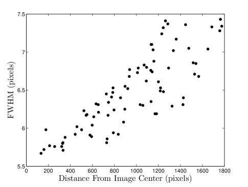
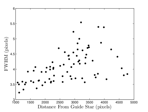
Figure 1.— PSF variation across the field for OPTIC data. Left: FWHM variation with distance from the field center in the image of J0110+6805 (observed without OT guiding). Right: variation with offset from the star used for rapid guiding near J0612+4122.

With the poorer seeing experienced during our MiniMo run, we found that the spatial variation of the PSF was much less important, with the FWHM varying by no more than a few $\sim 0.1$ pixels ($\sim 0.03^{\prime\prime}$) across the field of view. Again stacking errors were negligible. However for consistency we fit for and applied linear gradients in the PSF model.

Thus, in forming the final model PSF for the analysis, we were able to draw stars from across the fields avoiding only the outermost corners of the frames, where there was notable degradation. In general between $\sim$ 1/6 and $\sim$ 1/5 of the PSF stars used were saturated in their cores (only $\sim$ 1/9 with MiniMo, given the poorer seeing). Tables 2 and 3 list the number of PSF stars used in each image. The median number of PSF stars for each field was 30 for both OPTIC and MiniMo.

5. Host Galaxy Model Fitting

Previous studies (Scarpa et al., 2000; Urry et al., 2000; O’Dowd & Urry, 2005) indicate that BL Lac hosts are better fit by de Vaucouleurs profiles than exponential disks. We therefore adopt simple de Vaucouleurs profiles with fixed Sersic index 4, convolving the model with the image PSF, in our galaxy fitting. We did find examples of disturbed galaxies and hosts with faint companions, but no host appeared disk-dominated. Our BL Lac image model includes up to five parameters, introduced hierarchically. We start by fitting for nuclear (PSF) flux plus possible host. We assume that the host galaxy isophotes are centered on the nucleus (Falomo et al., 2000), and fit or bound the host flux, initially assuming a a fixed effective radius of $R_{\rm e}=1.64^{\prime\prime}$ (10  kpc at $z=0.5$; we assume $\Omega_{m}=0.3$, $\Omega_{\Lambda}=0.7$ and $H_{0}=70$ km s^-1 Mpc^-1 throughout this paper). We next allow the de Vaucouleurs profile $R_{\rm e}$ to vary, when required by a high significance for a measurement of $R_{\rm e}$ in the fit. Finally for a few BL Lacs, we find a significant detection of host ellipticity; in these cases we include the ellipticity $\epsilon$ and position angle $\theta$ as additional free parameters in the fit. After fitting the host normalization, we report galaxy magnitudes by extrapolating the integrated light to infinity.

To prepare for host fitting, we determine the centroid position of the core PSF, using the DAOPHOT task peak, which matches to the model PSF, excluding pixels above our (conservative) non-linearity threshold (30,000 ADU for OPTIC, 40,000 ADU for MiniMo), and delivering centroid coordinates accurate to $\pm 0.01$ pixels. Since a number of our images were saturated, this clipping was important for obtaining accurate centroids. In almost all cases, the galaxy surface brightness dropped below the background surface brightness fluctuations within our standard $5.6^{\prime\prime}$ PSF radius. Accordingly the BL Lac image model was fit to $11.2^{\prime\prime}\times 11.2^{\prime\prime}$ cutouts from the image stack centered on the BL Lac core pixel. DAOPHOT provides a 2$\times$-oversampled PSF model. This was re-binned to the original pixel size, using the precisely determined centroid and then used in the subsequent fitting. This PSF centering and re-sampling proved to be quite accurate – dipole structure was never evident in residuals to our final BL Lac model, whereas with even 0.05 pixel shifts for the BL Lac core position such residuals were obvious.

We apply our BL Lac fit to a subset of the pixels in the cutouts around each BL Lac. First all pixels beyond $5.6^{\prime\prime}$ (outside the PSF model) are masked. Pixels associated with resolved objects within the fitting radius but more than three FWHM from the BL Lac core are also masked (in practice we exclude rectangular regions, see Figure 2). Unresolved objects more than three FWHM away are fit to the PSF model and then treated as fixed background. Occasionally, very bright nearby stellar objects show significant residuals at the PSF core after subtraction; in these cases a few pixel rectangular region is masked at the core before the final BL Lac fit. The occasional column or pixel defect or cosmic ray are similarly masked. Finally we mask the pixels within 1 FWHM in diameter of the BL Lac core. In roughly 25% of the OPTIC images this was required in any case due to non-linear ADU levels. However, we found that sampling noise at 1 FWHM could dominate the fit statistics, so a consistent exclusion of pixels at the core was used for all objects. For a few of the brightest objects, we extended the core exclusion region to 1.5 FWHM, while for a few of the faintest, we used 0.5 FWHM. The final results were not sensitive to the precise value used.

For each BL Lac model the background was determined from an annulus starting at 7^′′ containing 2-3$\times$ the pixel count of the PSF model region; for a few poor seeing images and BL Lacs with very extended hosts we used a larger annulus.

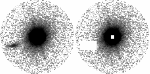
Figure 2.— Preparing the fitting region for J0814+6431 (image FWHM $0.45^{\prime\prime}$). One resolved companion and pixels near the centroid of the nuclear component are masked. The corrected FOV is $7.7^{\prime\prime}$ in radius; N up, E left.

5.1. Noise Model & $\chi^{2}$ Minimization

For all multi-parameter fits, the parameters are determined by minimization of the quantity:

$$\chi^{2}=\displaystyle\sum_{i}\frac{(I_{i}-M_{i})^{2}}{\sigma_{i}^{2}}$$ (1)

Where the sum is over the $\{i\}$ unmasked pixels in the fitting region, $I_{i}$ is the observed intensity in ADU, $M_{i}$ is the model intensity in ADU and $\sigma_{i}^{2}$ is the expected variance. The model is the sum of the constant background, PSF and host galaxy terms, where the analytic host model is integrated over a given pixel to determine the galaxy contribution. The variance is estimated according to simple Poisson statistics to be:

$$\sigma_{i}^{2}=\frac{I_{i}\times g+R^{2}}{g^{2}\times(n_{im}-1)}$$ (2)

Where for OPTIC the gain was $g=1.45\ e^{-}{\rm ADU}^{-1}$ and for MiniMo 1.4$\ e^{-}{\rm ADU}^{-1}$. The read noise $R$ is $R=4\ e^{-}$ (OPTIC) or 5.5$\ e^{-}$ (MiniMo) and our final image stack is the from the median of $n_{im}$ normalized single exposures. This is a simplification since for OPTIC the orthogonal transfer during integration correlated the sky noise (likely an artifact of imperfect flat-fielding). Also the residual pixel noise in the unmasked region adds to the variance for sharp images. Nevertheless we find that this variance is a reasonable first approximation to the local noise, and we can determine the best-fit model by $\chi^{2}$ minimization. We use the simulated annealing algorithm from Press et al. (1986).

The final size of the simplex in $N+1$ dimensions gives the relative errors between the $N$ estimates of the fitting parameters. We would like to relate this to the 1$\sigma$ statistical error, to provide a standard statistical error estimate for each parameter. We do this by scaling to an externally estimated 1$\sigma$ error determined for each point source flux $\sigma_{PSF}$.

5.2. Statistical Uncertainty

We determine this error by analogy with standard aperture photometry. In our case the central FWHM is masked in the fit so we compute the fractional error in the PSF amplitude for an annulus outside the masked region of width 1 FWHM as

$$f_{ann}=\frac{1}{N_{ann}}\times\sqrt{\frac{N_{ann}}{g\times(n_{im}-1)}+n_{ann}\times\sigma_{sky}^{2}+\frac{n_{ann}^{2}\times\sigma_{sky}^{2}}{n_{sky}}}$$ (3)

Where $N_{ann}$ is the source flux (ADU) within the photometry annulus, $n_{ann}$ is the number of pixels within the annulus, $\sigma_{sky}$ is the standard deviation of the background (ADU), and $n_{sky}$ is the number of pixels used to determine the background value. The first term under the radical is Poisson noise. The second is a statistical uncertainty due to the random fluctuations and unresolved sources in the background. The final term accounts for the possibility of a Poisson error in background level. The first term generally dominates, and thus $f_{ann}$ is $\sim\sqrt{2}\times f_{ap}$ as the annulus contains roughly 1/2 the flux of an aperture without the central mask. We found a typical $f_{ann}$ for our PSF stars of $\sim 1-2\times 10^{-3}$.

With the large number of counts for the point sources measured here, even small centroiding errors can in principle contribute to the error, since a varying fraction of the point source falls in the central masked pixels. To test for this in each PSF fit, we artificially shifted the model PSF position by $\pm 0.01$ pixels, the maximum centroiding error, in each coordinate. The rms variation in the included counts was computed to estimate $f_{cent}$, the fractional error in flux estimation due to imprecise centroiding. Although this error only became comparable to $f_{ann}$ for a few of the brightest point sources, we sum it in quadrature to compute our statistical photometry error as $\sigma_{PSF}=N_{PSF}\sqrt{(f_{ann}^{2}+f_{cent}^{2})}$, where $N_{PSF}$ is the total number of counts for the point source in ADU.

As noted above, the size and shape of the simplex determined from our $\chi^{2}$ minimization provides relative fitting errors. We adjusted our convergence criterion such that the rms spread about the mean fit value for the PSF amplitude was always close to $\sigma_{PSF}$ which, since the nuclear point source always dominates the model, is a very good estimate of the true model-fit statistical error. Thus, by rescaling the simplex amplitude such that the rms spread in the nucleus flux estimates was equal to this photometric error $\sigma_{PSF}$, we have normalized the simplex-determined error to be 1$\sigma$ (statistical) in each quantity. We call this error $\sigma_{\rm stat}$.

5.3. Systematic Uncertainty

Since our models are dominated by the bright core PSF, which is different for each exposure, and since we have a limited number of stars in each frame to generate a PSF model, our final uncertainty must be dominated by systematic errors due to imperfections in this model. This is in contrast to the HST-based fitting of Scarpa et al. (2000), where the PSF is, of course, stable and well-modeled and unresolved background structure dominated the final uncertainty. We therefore wish to estimate our systematic PSF uncertainty.

We do so by fitting for a de Vaucouleurs host around unresolved stellar sources. In each image stack we choose such test stars relatively close to the BL Lac with comparable brightness. On average we were able to measure seven such stars per image. Ideally none would have been used in forming the PSF, but since these are the stars most suitable for PSF modeling, they were largely included. Before fitting, each star was treated exactly as its associated BL Lac, including the same masking of central pixels. We then fit for the PSF amplitude and ‘host’ amplitude, with the de Vaucouleurs $R_{\rm e}=1.64^{\prime\prime}$ fixed at our default radius. The fit host amplitude could either be negative (indicating excess wings on the model PSF) or positive (PSF model too narrow). Note that decreasing the host angular size would weaken constraints on its amplitude, since it would be more highly covariant with the PSF. However, our adopted value (appropriate for a typical $R_{\rm e}=10$ kpc at $z=0.5$) is reasonably conservative; even at the minimum angular size at $z\sim 1.6$, this would only decrease by 28%.

The dispersion in the amplitudes of the fitted ‘host’ fluxes provides an estimate of our systematic uncertainty. However, since the stellar fluxes covered a substantial range, we elected to scale the ‘host’ flux significance to the statistical error on this flux for each test star $\sigma_{\rm stat}$ The rms spread in the ‘host’ fluxes fit around the test stars, in units of $\sigma_{\rm stat}$, then provides an estimate of the systematic error, for each individual BL Lac field. Figure 3 shows the distribution of ‘host’ significance ($N_{\rm host}/\sigma_{\rm stat}$) for the test stars in the OPTIC and MiniMo fields, along with the distribution of the rms significance for the individual fields.

The rms significance of these ‘host’ fits for OPTIC and MiniMo were 8.3$\sigma_{stat}$ and 8.0$\sigma_{stat}$, respectively. This suggests that our statistical (Poisson) errors on the host flux substantially underestimate the true errors by $\sim 8\times$. However, it should be noted that the distributions are approximately normal and that the mean fitted host flux is not significant. For the OPTIC data, we obtain $-0.7\sigma_{stat}$ while for MiniMo the average is 0.1$\sigma_{stat}$. In view of the systematic errors we expect random offsets of $\pm 0.6\sigma_{stat}$ and $\pm 0.7\sigma_{stat}$ for the two sets of test stars. We conclude that the frame-to-frame spread in upper limits on surrounding host galaxies are appreciably larger than expected from pure Poisson statistics – this can be attributed to errors in forming the individual PSF models and to unresolved structure in the PSF stars’ and test stars’ backgrounds. However there is no overall introduced host flux; implying that our PSF model is a fair, albeit uncertain, representation of the data.

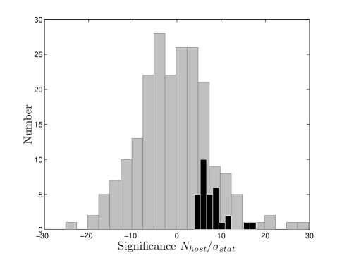
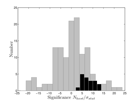
Figure 3.— Statistical significance of ‘host’ detections around field stars. Left: OPTIC stars for 31 fields, Right: MiniMo stars for 18 fields. The dark histograms show the distribution of the rms significances for the individual BL Lac fields. There is a modest tail, but most cluster near the global rms. These individual rms values give our systematic error estimates for the individual BL Lac fields.

To be conservative, we adopt for our final error the sum of the statistical and systematic errors, namely $\sigma_{fin}=\sigma_{stat}(1+\sigma_{syst})$, where $\sigma_{syst}=(N_{host}/\sigma_{stat})_{rms}$ is the rms value of the individual test stars in the stacked image of an individual BL Lac. This is conservative since while we expect the statistical errors to have a normal distribution, it would be very surprising if the much larger systematic errors had wings as large as a Gaussian out to many times the FWHM of the distribution. We tested this error estimate by inserting Poisson realizations of model hosts around isolated stars in several fields. For artificial galaxies assigned the total counts at the 3$\sigma_{fin}$ detection limit, we recovered host fluxes with rms errors of $0.7\sigma_{fin}$. In no case was the difference between the injected and recovered counts larger than $1\sigma_{fin}$.

5.4. Final BL Lac Fitting Procedure

We constrain the properties of the BL Lac host by the hierarchical fit. We first fit for a circularly symmetric host with fixed angular radius $R_{\rm e}=1.64^{\prime\prime}$, just as for the test star measurements. The final uncertainty on the host counts is taken to be $\sigma_{fin}$ where the statistical error is taken from the simplex rescaled to the aperture photometry error for the BL Lac core, while the systematic error is the multiple of this statistical error determined by ‘host’ fits to the test stars in this BL Lac’s field, as described above. If the host flux is larger than $3\sigma_{fin}$ (which is dominated by the systematic uncertainty), we deem it significant. If the significance does not reach $3\sigma_{fin}$, we infer an upper limit of $N_{host}+3\sigma_{fin}$, or $3\sigma_{fin}$, whichever is larger.

If there is a significant detection of a BL Lac host, we next re-run the fits allowing the host angular radius $R_{\rm e}$ to vary. The only fitting constraint is $R_{\rm e}>0$. If the best fit value of $R_{\rm e}$ is less than the FWHM for the image, we do not deem it significant. A value for $R_{\rm e}$ is only quoted if $R_{\rm e}>3\sigma_{fin}$, where the final statistical plus systematic error is estimated from the re-scaled simplex, as above. Significant estimates of $R_{\rm e}$ were found for 25% of the OPTIC-measured BL Lacs and 33% of those measured with MiniMo. Note that the overall flux and its fit error were free to vary, as well. As a consistency check, we note that in no case where a significant $R_{\rm e}$ measurement was found, did the host flux measurement decrease in significance to below $3\sigma$.

Finally, we attempted to fit for a significant host ellipticity, with two additional parameters $\epsilon$ and the position angle $\theta$ added to the model. These parameters both exceeded $3\sigma_{fin}$ significance for only two of the BL Lacs observed with OPTIC. Again the host flux and size $R_{\rm e}$ were free in this final fit.

Tables 2 and 3 contain the final fit nucleus and host amplitudes (converted to magnitudes, see below) and the host physical size (when available). Details of the observations (exposure lengths, FWHM of the stellar sources and the number of stars used in the PSF model) are also listed.

6. Redshift Estimates & Lower Limits

Since Sbarufatti et al. (2005) have argued that BL Lac host galaxies are standard candles with $M_{R}=-22.9\pm 0.5$, we can use our measurements and upper limits on the host flux to extract redshift estimates and lower bounds. To do this we compute an $i^{\prime}$ Hubble diagram for our KPNO 1586 filter. We improve on the similar R-band Hubble diagram of Sbarufatti et al. (2005), by including host evolution, assuming a host (elliptical) formation redshift of $z_{form}=2$ (O’Dowd & Urry, 2005). With this assumption, we adopt an elliptical galaxy spectrum computed at the appropriate age from the PEGASE model of Fioc & Rocca-Volmerange (1997), where the age is computed for each $z_{obs}<z_{form}$ for our standard cosmology. To lock the overall normalization to the $M_{R}$ of Sbarufatti et al. (2005), we fixed the flux of the $z=0$, evolved elliptical spectrum to $M_{R}=-22.9$. This required folding through an $R$ filter. Unfortunately the precise KPNO Kron-Cousins $R$ filter used is not recorded, except in a private 1995 communication between J. Holtzman and Landolt (Holtzman et al., 1995). Accordingly we use the transmission curve for Kron-Cousins R filter KPNO w004, first obtained in 1994; this may be the precise filter used in the original study. In any case, after normalizing with this filter at $z=0$, we take the model flux from each observation redshift, convert to the observed frame using the luminosity distance $d_{L}$ from our standard cosmology and convolve with the $i^{\prime}$ KPNO 1586 transmission (Figure 5) to obtain the apparent magnitude.

The resulting Hubble diagram is shown in Figure 5. For comparison we have also computed the $R$-band Hubble diagram for this evolving model. The curve is quite close to Sbarufatti et al. (2005)’s analytic approximation, although departures caused by the evolution are evident. Hubble diagram computations with other evolving galaxy models yielded similar curves, with differences small compared to those introduced by uncertainty in the host absolute magnitude.

To compare with our measurements, we converted our model fit host counts (in ADU) to $i^{\prime}$ magnitudes, including atmospheric (Massey et al., 2002) and Galactic (Schlegel et al., 1998) extinction corrections. The establishment of the flux scale is discussed above (§3), while the assumed Galactic extinctions from the dust maps at the BL Lac locations are listed in Tables 2 and 3.

Finally, these host magnitudes (and lower limits) are converted to redshifts using our Hubble diagram. Of course the host absolute magnitude uncertainty translates into a range of possible redshifts. There are two contributions to the full redshift uncertainty. The first is host measurement uncertainty, including both statistical and systematic photometry errors. We use the $\pm\sigma_{fin}$ range for the maximum and minimum host magnitude to infer asymmetric error bars on the host redshifts. This is augmented by adding, in quadrature, the photometry errors estimated for our zero point – this increase is however very small. These values are listed as the first error flags in the final columns of Tables 2 and 3. In addition, the claimed $\delta R=0.5$ mag dispersion in the host luminosity leads to a redshift range. We propagate the $z=0$ $R$ absolute magnitude uncertainty through observed $i^{\prime}$ and hence to $\Delta z$ as a function of redshift (see Figure 6). This nearly always completely dominates the redshift uncertainty and is listed as the second error flag in our tables.

For objects with a fit angular $R_{\rm e}$, the central redshift estimate is used to convert to proper kpc; the values are comfortably close to the otherwise assumed $R_{\rm e}=10$ kpc. Finally, for undetected hosts, we take the minimum $z$ allowed by the $3\sigma_{fin}$ host magnitude limit, the photometric scale errors, and the standard value for the host luminosity to obtain a lower limit on the host redshift. Again this is listed in the last column of Tables 2 and 3.

We have treated our measurement errors conservatively, having summed the systematic and statistical uncertainties in our error flags and requiring $3\times\sigma_{fin}$ detections before claiming a measurement is significant. On the other hand, we consider only the assumed dispersion in the host luminosity. Clearly an improved calibration of the host magnitudes (if uniform) can make these measurements much more useful.

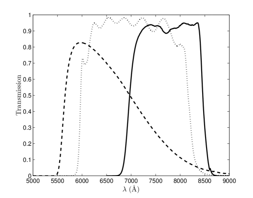
Figure 4.— Filter transmission curves used in this study. Solid $i^{\prime}$, dashed $R$, dotted HST F702W. We convert from the assumed host $z=0$ $R$ magnitude to our observed $i^{\prime}$ magnitude. Note that the $i^{\prime}$ cut-on is redder than used in previous studies.

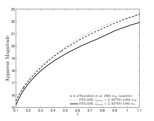
Figure 5.— Hubble diagrams calculated in KPNO w004 $R$ and KPNO 1586 $i^{\prime}$. The analytic estimate for the $R$ Hubble diagram of Sbarufatti et al. (2005) is shown for comparison.

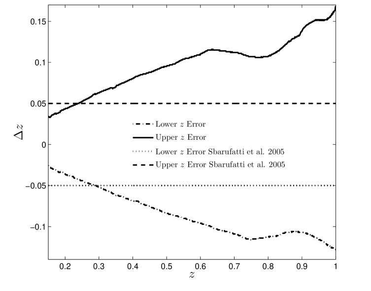
Figure 6.— Upper and lower error error bars as a function of redshift, inferred from the $\pm 0.5$ dispersion in host absolute magnitude $M_{R}$ at $z=0$.

7. Results and Discussion

We were able to detect hosts for 14/31 OPTIC-observed BL Lacs and 11 of 18 observed with MiniMo. The redshift estimates varied from $\sim 0.20-0.95$ and the lower limits from $\sim 0.25-0.9$. For OPTIC the median value was $z=0.54$ for MiniMo $z=0.53$. It is interesting to compare this with the HST  host detections of Scarpa et al. (2000); in this study nearly all BL Lacs at $z<0.5$ were resolved but only 6/23 sources with known $z>0.5$ yielded host detections. While at first sight it might seem surprising that a ground-based program could be competitive, it should be remembered that the HST snapshot BL Lac survey observed with the F606W and F702W filters. The $i^{\prime}$ filter blue cut-on is $\sim 100$ nm redder than for the bulk of the HST observations, and so we do not expect to suffer appreciable surface brightness attenuation from the 4000Å  break until $z\sim 0.75$. Further the typical HST snapshot exposures were $\sim 500$ s with a 2.4 m aperture $vs.$ 900$-$2100 s with a 3.6 m aperture. The combination of redder band and deeper exposure allow some additional sensitivity to the low surface brightness host wings. Of course, our sources were selected from those lacking spectroscopic redshifts, making it likely that these are a higher redshift sub-sample. However it is also worth noting that the typical $\sim 10-30\times$ core host ratio plotted in Figure 7 represents an even stronger core dominance, compared to the HST  sample, than one might think since the continua of BL Lacs is quite blue compared to the hosts, and our $i^{\prime}$ bandpass is redder than that of previous $R$ or $F606W/F702W$ studies.

Figure 7.— Host magnitude $vs.$ nucleus magnitude. The dashed lines show hosts $10\times$ and $100\times$ fainter than the BL Lac nucleus.

For 14 of the 25 detected hosts we obtained estimates of the host angular size. The inferred median effective radii were 9.2 kpc (OPTIC) and 8.0 kpc (MiniMo) in good agreement with previous BL Lac host estimates (Scarpa et al., 2000; Urry et al., 2000; Falomo et al., 2000). The other detected hosts had $R_{\rm e}$ measurements with $<3\sigma_{fin}$ significance or best fit radii smaller than the FWHM and thus were judged to be insignificantly resolved.

In two cases we have a formal detection of ellipticity. For J0211+1051 the small value $\epsilon=0.21$ accords well with the visual impression (Figure 11). In the other case, J0348$-$1610, the ellipticity is also small $\epsilon=0.14$, but here the result is suspect, as there is a bright companion within $2R_{\rm e}$. Indeed it may be no coincidence that the two objects with significant $\epsilon$ both have a large number of companions. While the upper limits on $\epsilon$ are in some cases constraining, we conclude that with our modest ground-based resolution we cannot in most cases probe the host structure.

One arena where the comparison with HST-based measurements should be fairly robust is the host-nucleus flux ratio. Here we find a marked difference with the HST sample. Of the 69 BL Lac hosts resolved by Scarpa et al. (2000), 54% of these had $f_{host}/f_{nucleus}\gtrsim 1$. Even counting the 42 unresolved BL Lacs 34% had a nuclear-host ratio $\gtrsim 1$. In contrast, we find only 1 object of our 49 BL Lacs has $f_{host}/f_{nucleus}>1$. Indeed 63% of our hosts are $\geq 10\times$ fainter than the nucleus (Figure 7). Two selection effects may account for this difference. First, these objects have been selected as bright flat spectrum radio core sources. Further a significant fraction of the MiniMo targets were in addition known to be active gamma-ray emitters. This implies that the Earth line-of-sight is even more nuclear component dominated (on-axis) than for the typical BL Lac. Second, these are the subset of these systems lacking previous spectroscopic redshifts. Again, this suggests that they should be even more core continuum dominated than the typical BL Lac.

7.1. Radial Profile Plots

We present here a sample of azimuthally averaged $i^{\prime}$ instrumental surface brightness plots, compared with our best fit model components (Figures 8 $-$ 10). The surface brightness data are measured from excess counts above the above the fitted background level measured in annuli about the core position. The model curves are from integrations over these radial bins. The error bars shown are 1$\sigma$, calculated in a fashion consistent with the variance in §5. We show two BL Lacs with host detections using the OPTIC camera, as well as two fits providing upper limits. For MiniMo we show one detected host and one unresolved source.

 

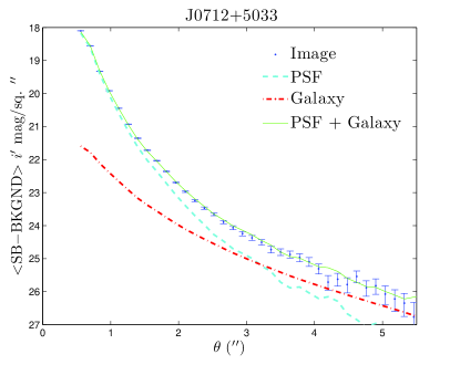
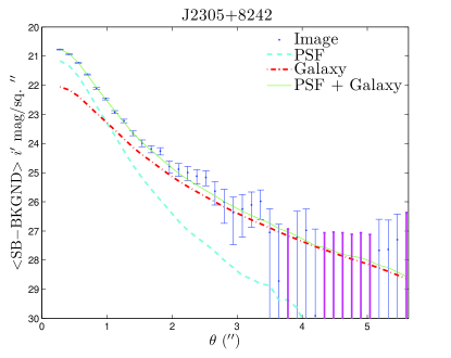
Figure 8.— OPTIC radial profiles for fit BL Lacs: Left: J0712+5033, resolved at $z\approx 0.47$. Right: J2305+8242, resolved at $z\approx 0.62$. The dashed lines show the PSF, the dot-dashed lines the host and the solid line the total model. Error flags on individual radial bins are statistical only.

 

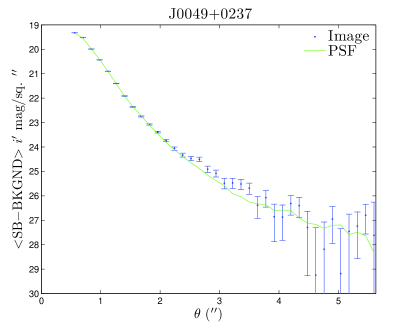
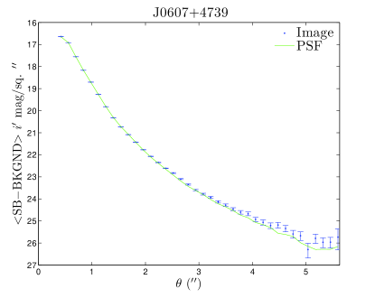
Figure 9.— OPTIC radial profiles for fit BL Lacs with host non-detections: Left: J0049+0237, unresolved $z>0.84$. Right: J0607+4739, unresolved $z>0.54$.

 

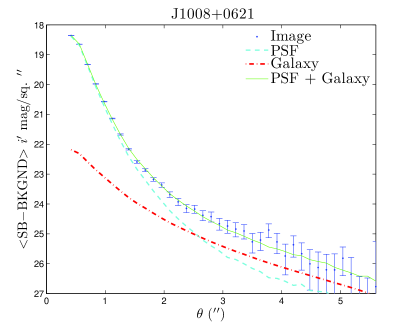
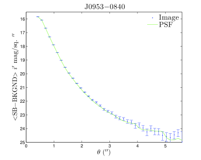
Figure 10.— MiniMo radial profiles for fit BL Lacs. Left J1008+0621, resolved at $z\approx 0.59$. Right: J0953$-$0840, unresolved $z>0.40$.

7.2. Near Environments

It has been noted (Scarpa et al., 2000; Urry et al., 2000; Falomo et al., 2000) that BL Lac hosts are surrounded by a significant excess of nearby galactic objects. Following O’Dowd & Urry (2005), we count companions within a projected proper distance of 50 kpc of the BL Lac centroid. When we do not have a $z$ estimate, we count only companions within $5.9^{\prime\prime}$ of the nucleus (50 kpc at the minimum angular diameter distance $z\sim 1.6$). We count only resolved objects.

We find at least one companion for 51% of our BL Lacs (25/49), in reasonable agreement with the detection rate of Urry et al. (2000) (47%) and O’Dowd & Urry (2005) (62.5%). Of course, with our ground-based imaging, some of the unresolved nearby sources may represent additional compact galactic companions. The number of companions $N_{c}$ within a projected distance of $r_{\perp}=50$  kpc, the magnitudes of the two brightest companions (and the comparison of the brightest to the host flux $\Delta m_{1,host}$) and a flag indicating evidence for interaction are given in Table 1. As noted above, our two hosts with nominal detections of ellipticity have both large numbers of nearby companions and morphological evidence for interaction. These may in fact represent recent mergers in compact groups. J1440+0610 has an extended companion with centroid at $r_{\perp}>50$ kpc which extends within 50 kpc. For two objects (J0050$-$0929 and J0743+1714) the companion at small radius may be physically contiguous with the undetected host. Clear evidence for interaction was seen only for the better-seeing OPTIC data, so additional companion interaction is likely.

Name	$N_{c}$	$m_{i^{\prime},1}$	$m_{i^{\prime},2}$	$\Delta m_{1,host}$	$r_{min}$ (′′)	$r_{min}$ (kpc)	Int.?
J0050$-$0929	1	$>$ 19.5	-	-	$<$ 0.6	-	M
J0202+4205	1	22.7	-	1.3	4.1	33	N
J0203+7232	1	22.3	-	-	5.6	-	N
J0211+1051	7	21.9	23.6	5.0	7.3$\dagger$	24$\dagger$	Y
J0219$-$1842	1	21.5	-	1.7	3.6	25	Y
J0348$-$1610	5	21.5	21.6	2.9	2.7	14	Y
J0607+4739	1	23.0	-	-	4.6	-	Y
J0610$-$1847	1	23.3	-	3.2	4.9	35	N
J0625+4440	2	22.5	24.2	-	3.8$\dagger$	-	M
J0650+2502	2	21.6	22.5	2.6	5.3$\dagger$	31$\dagger$	N
J0743+1714	2	$>$ 21.8	23.7	-	$<$ 0.6	-	M
J0814+6431	1	22.3	-	3.9	5.2	25	M
J0817$-$0933	2	22.4	23.8	2.0	4.9$\dagger$	35$\dagger$	N
J0835+0937	1	22.2	-	-	3.8	-	M
J0907$-$2026	1	21.9	-	3.6	8.0	39	N
J0915+2933	1	22.1	-	3.7	9.4	47	N
J1008+0621	3	22.1	23.7	2.3	4.1	27	M
J1243+3627	1	23.9	-	4.6	4.1	25	M
J1253+5301	1	24.1	-	4.3	7.5	50	M
J1427+2347	1	22.7	-	5.4	8.1	30	M
J1440+0610	1	20.2	-	0.6	8.1	64	N
J1542+6129	1	22.8	-	4.1	7.7	40	M
J1624+5652	1	23.0	-	2.1	5.0	35	N
J2241+4120	2	22.6	23.0	3.5	2.8$\dagger$	18$\dagger$	Y
J2305+8242	1	23.1	-	3.1	5.6	42	N

Table 1 List of brightest observed companions within $r_{\perp}=50$ kpc. Except for those marked $\dagger$, the brightest companion is also the closest. We classify the morphological evidence for interaction as obvious “Y,” possible “M” or absent “N.”

 

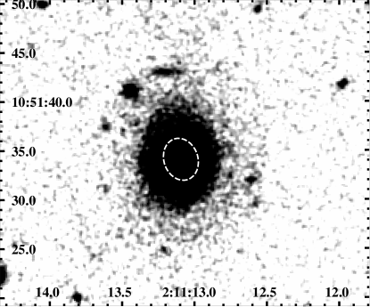
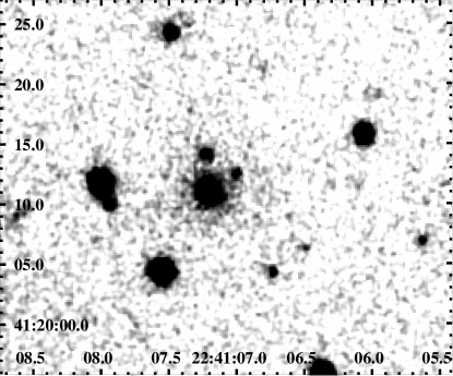
Figure 11.— Two BL Lac fields after core PSF subtraction. Left: J0211+1051 at $z\approx 0.20$, showing the highly resolved host and several fainter companions. The host has significant ellipticity; the fit $R_{\rm e}$ ellipse is shown. Right: J2241+4120 at $z\approx 0.52$, showing the faint wings of the host and two fainter companions. No significant ellipticity is detected.

7.3. Comparison with Other Redshift Estimates

As a part of our on-going spectroscopic campaign to obtain identifications and redshifts for the Fermi-detected blazars, some of these imaging targets have had additional spectroscopic exposure. In a few cases we obtain true spectroscopic redshifts $z_{s}$. In several other cases we have lower limits on the redshift $z_{abs}$ from detection of intervening intergalactic absorption-line systems. Finally, in several cases we were able to use spectroscopic limits on absorption line-strengths (typically Ca H & K and G-band limits), together with the assumption of a uniform host magnitude (as in this paper) to place lower redshift limits $z_{HK}$ on the BL Lac (Shaw et al., 2009).

We have obtained a direct redshift measurement for only one of these targets, using Keck LRIS spectroscopy (Shaw et al., 2010). The value is within $1\sigma$ (statistical+systematic) of the imaging estimate:

J2022+7611 $z_{I}=0.49^{+0.04+0.09}_{-0.03-0.08}$ ($z_{s}=0.584$).

For three objects our imaging $z_{I}$ estimates are in agreement with lower limits from our own spectroscopy (Shaw et al., 2009). The low redshift of J1427+2347 is particularly interesting in view of the recent VERITAS TeV detection of this source (Ong et al. 2009).

J0712+5033 $z_{I}=0.47^{+0.03+0.09}_{-0.02-0.08}$ ($z_{HK}>0.47$).

J1427+2347 $z_{I}=0.23^{+0.01+0.05}_{-0.01-0.04}$($z_{HK}>0.03$).

J1440+0610 $z_{I}=0.55^{+0.02+0.10}_{-0.02-0.09}$($z_{abs}>0.316$).

For two objects our imaging redshift constraints are stronger than those obtained from the spectroscopic constraint on the HK line strengths:

J0909+0200 $z_{I}>0.83$ ($z_{HK}>0.54$, Shaw et al. (2009).

J0049+0237 $z_{I}>0.84$ ($z_{HK}>0.82$ Sbarufatti et al. (2006).

For two objects our lower limit on the redshift from imaging is not as strong as that from our spectroscopy (Shaw et al., 2009):

J0050$-$0929 $z_{I}>0.27$ ($z_{HK}>0.44$) and

J2050+0407 $z_{I}>0.74$ ($z_{abs}>0.819$).

Finally for two objects the imaging redshifts are in disagreement with the lower limits from limits on the HK absorption line strength:

J1253+5301 $z_{I}=0.59^{+0.02+0.11}_{-0.02-0.10}$ ($z_{HK}>0.77$; $1.4\sigma$ higher) and

J1542+6129 $z_{I}=0.39^{+0.03+0.08}_{-0.03-0.07}$ ($z_{HK}>0.63$; $2.2\sigma$ higher).

These last two disagreements may partly be attributed to differences in the host size and slit losses assumed in the spectroscopic method. However, statistically we should expect some $z_{I}$ estimates to be low, as Malmquist bias will assure that fluctuations causing detections make the sources appear artificially close. Of course it is also likely that outliers in the BL Lac host magnitude distribution exist: these will cause larger disagreements. As we continue to collect spectroscopic redshifts and limits for these sources, we should be able to probe the fraction of sub-luminous hosts and test the utility of the standard candle hypothesis of Sbarufatti et al. (2005).

8. Conclusions

We have detected hosts for half of the BL Lac objects imaged in this WIYN campaign. These detections, assuming a standard host luminosity, give redshift estimates with a median value of $z_{\rm med}=0.51$. The upper limits on host flux for the remaining objects also give reasonable redshift constraints with a median value for the bound of $z_{\rm med}>0.61$. This may be compared with the spectroscopic redshifts already obtained for the two parent BL Lac populations: for the BL Lacs in the early Fermi blazar list one finds $z_{\rm med}=0.33$, while for the radio selected CGRaBS BL Lacs, we have $z_{\rm med}=0.45$ (Figure 12). We can further quantify the difference by making Kolmogorov-Smirnoff comparisons of the distributions. While the LBAS and CGRaBS sets are quite consistent, with a KS probability of 0.58, the imaging set differs from both with a KS probability of similarity of only $1-5\times 10^{-3}$. If we include the lower $z$ bounds in the distribution the probability drops to $<2\times 10^{-5}$.

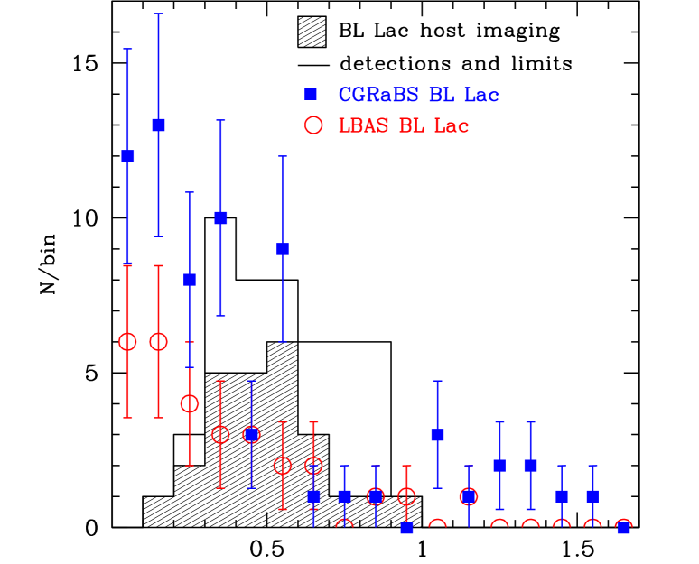
Figure 12.— BL Lac redshift distributions. Estimates from host detections (filled histogram), and with host lower limits (line histogram). For comparison we also show the spectroscopic BL Lac redshift distribution from the two parent populations providing our target lists: Squares – the CGRaBS flat spectrum radio loud BL Lacs (Healey et al., 2008) and Circles – the early Fermi gamma-ray-detected BL Lacs (Abdo et al., 2009a).

The evident lack of low redshift imaging detections is doubtless a selection effect: such objects will in general show the strongest absorption features from the host and thus are most likely to provide spectroscopic redshifts. With the ground-based imaging results, we obtain a number of additional redshift estimates, with good efficiency for host detection out to $z\sim 0.65$. The distribution of our upper limits suggests that space-based imaging searches, using near-IR filters, can be productive to even higher redshift. In any event, it appears that it would be a mistake to assume that the objects in the radio and gamma-ray samples lacking spectroscopic redshifts are similar to those with spectroscopic distances. The imaging results suggest, in contrast, that these other sources are appreciably more distant and, on average have higher luminosity. It will be important to include these imaging $z$ estimates and bounds in attempts to measure the BL Lac luminosity function.

One other major conclusion of this analysis is that host searches should be at the $i$ band or redder. Here the contrast with the relatively blue nuclear continuum flux is improved: we have seen that this allows host detections in sources with extreme core dominance. The increased sensitivity to the low surface brightness halos of the redshifted hosts should also materially improve the detection fraction at $z>0.5$. Again this will be important for study of the population and evolution of BL Lac hosts galaxies. Finally, it will be important to pursue spectroscopic confirmations of these redshift estimates, as only with such data will it be possible to test and extend the claimed uniformity of the BL Lac host population and to probe its possible evolution.

Name	Exposures (s)	Seeing (′′)	$b\ (^{\circ})$	AI	N${}_{PSF\ stars}$	$i^{\prime}_{nucleus}$	$i^{\prime}_{host}$	$f_{host}/f_{nucleus}$	$R_{\rm e}$ (kpc)	$z$
J0004$-$1148	[180,180,300,300,300]	0.74	$-71.1$	0.06	25	19.66	$>$ 21.02	$<$ 0.28	-	$>$ 0.86
J0049+0237	[300,300,300,300,300]	1.04	$-60.3$	0.05	29	17.92	$>$ 20.97	$<$ 0.06	-	$>$ 0.84
J0050$-$0929	[60,60,60,60,60,60,60,60,60]	0.59	$-72.4$	0.06	13	15.31	$>$ 17.65	$<$ 0.12	-	$>$ 0.27
J0110+6805	[180,180]	0.76	5.29	2.38	61	14.48	17.90${}_{-.28}^{+.36}$	0.04	-	0.29${}_{-.03-.05}^{+.03+.06}$
J0202+4205	[180,300,300,300,300]	0.46	$-18.9$	0.18	24	18.05	21.39${}_{-.31}^{+.42}$	0.05	$13.9\pm 1.58$	0.94${}_{-.07-.11}^{+.13+.15}$
J0203+7232	[180,180,180]	0.49	10.4	1.37	52	16.21	$>$ 18.64	$<$ 0.11	-	$>$ 0.39
J0211+1051	[60,60,60,180,180,180]	0.50	$-47.4$	0.27	27	15.32	16.91${}_{-.09}^{+.09}$	0.23	$6.34\pm 0.17$	0.20${}_{-.01-.04}^{+.01+.04}$
J0219$-$1842	[180,180,180,180,180]	0.76	$-68.1$	0.07	20	17.65	19.85${}_{-.16}^{+.18}$	0.14	-	0.60${}_{-.03-.10}^{+.04+.11}$
J0348$-$1610	[180,180,180,180,180]	0.70	$-47.6$	0.09	24	16.67	18.65${}_{-.07}^{+.07}$	0.16	$11.1\pm 2.33$	0.39${}_{-.01-.07}^{+.01+.08}$
J0433+2905	[180,180,300,300,300]	0.46	$-12.6$	1.49	30	17.53	$>$ 19.20	$<$ 0.21	-	$>$ 0.48
J0502+1338	[300,300,300,300,300]	0.49	$-16.8$	0.99	28	18.18	19.05${}_{-.08}^{+.08}$	0.44	$8.87\pm 1.73$	0.45${}_{-.01-.08}^{+.01+.09}$
J0509+0541	[60,60,60,60,60]	0.53	$-19.6$	0.21	28	14.75	$>$ 18.60	$<$ 0.03	-	$>$ 0.38
J0527+0331	[300,300,300,300,300,300,300]	0.67	$-16.9$	0.31	27	18.64	21.24${}_{-.17}^{+.19}$	0.10	$4.91\pm 1.63$	0.90${}_{-.04-.11}^{+.05+.14}$
J0607+4739	[180,180,180,180,180,180]	0.78	12.9	0.36	30	15.53	$>$ 19.56	$<$ 0.02	-	$>$ 0.54
J0610$-$1847	[180,180,180]	0.83	$-17.3$	0.17	24	17.45	20.07${}_{-.31}^{+.42}$	0.09	-	0.64${}_{-.06-.10}^{+.10+.12}$
J0612+4122	[130,90,120,120,120]	0.50	$10.9$	0.39	28	16.67	$>$ 20.28	$<$ 0.04	-	$>$ 0.69
J0625+4440	[180,180,180,180,180]	0.60	14.4	0.29	23	17.12	$>$ 20.60	$<$ 0.04	-	$>$ 0.77
J0712+5033	[240,120,120,120]	0.60	23.9	0.13	28	16.42	19.17${}_{-.14}^{+.16}$	0.08	$8.68\pm 1.83$	0.47${}_{-.02-.08}^{+.03+.09}$
J0814+6431	[90,90,90,90,90]	0.45	33.2	0.12	26	15.51	18.38${}_{-.09}^{+.10}$	0.07	$11.4\pm 3.06$	0.35${}_{-.01-.06}^{+.01+.07}$
J0909+0200	[180,180,180,180,180]	0.52	31.4	0.06	28	17.90	$>$ 20.91	$<0.06$	-	$>$ 0.83
J1813+0615	[180,180,180]	0.83	11.3	0.41	106	17.40	$>$ 20.31	$<$ 0.07	-	$>$ 0.70
J190311+554044	[120,120,120,120]	0.53	20.5	0.12	36	16.27	$>$ 19.75	$<$ 0.04	-	$>$ 0.58
J1927+6117	[120,120,120,120,120]	0.69	19.5	0.13	70	16.95	19.57${}_{-.10}^{+.11}$	0.09	-	0.54${}_{-.02-.09}^{+.02+.10}$
J2009+7229	[180,180,180,180,180]	0.66	20.2	0.53	30	17.23	$>$ 20.50	$<$ 0.05	-	$>$ 0.74
J2022+7611	[180,180]	0.64	21.1	0.47	37	16.68	19.26${}_{-.18}^{+.21}$	0.09	-	0.49${}_{-.03-.08}^{+.04+.09}$
J2050+0407	[180,180,180,180,180]	0.83	$-24.0$	0.18	29	17.93	$>$ 20.48	$<$ 0.10	-	$>$ 0.74
J2200+2137	[300,300,300,300,300]	0.67	$-26.0$	0.20	32	18.50	$>$ 20.64	$<$ 0.14	-	$>$ 0.77
J2241+4120	[300,300,300,300,300]	0.70	$-15.2$	0.47	31	17.68	19.46${}_{-.11}^{+.12}$	0.19	$9.60\pm 1.00$	0.52${}_{-.02-.09}^{+.02+.10}$
J224356+202101	[90,60,60]	0.56	$-33.4$	0.09	39	15.10	$>$ 18.64	$<$ 0.04	-	$>$ 0.39
J2305+8242	[300,300,300]	0.94	$20.6$	0.46	31	19.99	19.97${}_{-.15}^{+.15}$	1.03	-	0.62${}_{-.03-.10}^{+.04+.12}$
J2346+8007	[300,300,300,300]	1.01	$17.6$	0.45	68	17.90	$>$ 21.07	$<$ 0.14	-	$>$ 0.87

Table 2 Summary of OPTIC results. 4+4 names are from CGRaBS (Healey et al., 2008), 6+6 names are from CRATES (Healey et al., 2007). There are also two $>3\sigma$ dectections of host ellipticity: J0211+1051 with $\epsilon=0.21\pm 0.02$ at $\theta=19^{\circ}\pm 10^{\circ}$ and J0348$-$1610 with $\epsilon=0.14\pm 0.04$ at $\theta=32^{\circ}\pm 15^{\circ}$ with angles measured N through E.

Name	Exposures (s)	Seeing (′′)	$b\ (^{\circ})$	AI	N${}_{PSF\ stars}$	$i^{\prime}_{nucleus}$	$i^{\prime}_{host}$	$f_{host}/f_{nucleus}$	$R_{\rm e}$ (kpc)	$z$
J024330+712012	[300,300]	1.09	10.4	1.50	51	16.95	$>$ 18.70	$<$ 0.20	-	$>$ 0.40
J065047+250304	[60,300,300,300,300]	0.68	11.0	0.19	31	16.14	19.03${}_{-.10}^{+.11}$	0.07	-	$0.45_{-.02-.08}^{+.02+.09}$
J0743+1714	[300,300,300]	0.65	19.0	0.07	41	18.43	$>$ 20.82	$<$ 0.11	-	$>$ 0.81
J0817$-$0933	[300,300,300,300]	0.78	14.3	0.20	42	16.61	20.37${}_{-.18}^{+.21}$	0.03	$12.5\pm 0.58$	0.71${}_{-.04-.11}^{+.05+.11}$
J083543+093659	[300,300,300]	0.83	27.5	0.10	30	17.93	$>$ 18.89	$<$ 0.41	-	$>$ 0.42
J0907$-$2026	[300,300,300]	0.97	18.0	0.34	35	14.46	18.32${}_{-.20}^{+.25}$	0.03	$8.05\pm 0.39$	$0.34_{-.03-.06}^{+.03+.07}$
J091553+293326	[300,300,300]	0.68	42.9	0.05	23	15.71	18.45${}_{-.16}^{+.19}$	0.08	$8.50\pm 0.16$	$0.36_{-.02-.06}^{+.03+.07}$
J095301$-$084034	[300,300,300]	0.78	33.9	0.92	34	15.29	$>$ 18.71	$<$ 0.04	-	$>$ 0.40
J1008+0621	[300,300,300]	0.73	46.0	0.05	26	17.68	19.80${}_{-.13}^{+.14}$	0.14	$14.8\pm 4.32$	$0.59_{-.03-.10}^{+.03+.11}$
J103742+571158	[300,300,300,300,300]	0.76	51.8	0.01	20	15.97	$>$ 19.95	$<$ 0.03	-	$>$ 0.62
J105912$-$113424	[300,300,300]	0.85	42.7	0.05	21	15.86	$>$ 19.08	$<$ 0.05	-	$>$ 0.46
J124313+362755	[300,300,300,300]	0.86	80.5	0.02	26	15.72	19.32${}_{-.20}^{+.24}$	0.04	-	$0.50_{-.04-.08}^{+.04+.10}$
J125311+530113	[300,300,300,300,300]	0.93	64.1	0.02	22	16.83	19.83${}_{-.08}^{+.08}$	0.06	$7.37\pm 0.73$	$0.59_{-.02-.10}^{+.02+.11}$
J142700+234802	[300,300,300]	0.71	68.2	0.11	28	13.99	17.30${}_{-.06}^{+.06}$	0.05	-	$0.23_{-.01-.04}^{+.01+.05}$
J144052+061033	[300,300]	0.98	56.6	0.07	26	16.89	19.59${}_{-.10}^{+.11}$	0.08	$7.24\pm 2.31$	$0.55_{-.02-.09}^{+.02+.10}$
J154225+612950	[300,300,300]	1.02	45.4	0.03	33	14.98	18.68${}_{-.17}^{+.20}$	0.03	-	$0.39_{-.03-.07}^{+.03+.08}$
J1624+5652	[300,300,300]	0.89	42.3	0.02	33	17.93	20.07${}_{-.17}^{+.20}$	0.14	-	$0.64_{-.04-.10}^{+.05+.12}$
J1749+4321	[300,300,300]	1.09	29.2	0.07	30	17.41	$>$ 20.73	$<$ 0.05	-	$>$ 0.79

Table 3 Summary of MiniMo results. 4+4 names are from CGRaBS (Healey et al., 2008), 6+6 names are from CRATES (Healey et al., 2007). No {$\epsilon$, $\theta$} was found with significance $>3\sigma$ for any BL Lac in these data.

References

- Abdo et al. (2009a) Abdo, A.A. et al., 2009a, ApJ, 700, 597
- Abdo et al. (2009b) Abdo, A.A. et al., 2009b, ApJS, 183, 46
- Abdo et al. (2010) Abdo, A.A. et al., 2010, ApJ, subm.
- Davis (1994) Davis, L. 1994, “A Reference Guide to the IRAF/DAOPHOT Package”
- Falomo et al. (2000) Falomo, R. et al. 2000, ApJ, 542, 731
- Fioc & Rocca-Volmerange (1997) Fioc, M. & Rocca-Volmerange, B. 1997, AA, 326. 950
- Hartmann et al. (1999) Hartmann, R.C. et al. 1999, ApJS, 123, 79
- Healey et al. (2007) Healey, S.E. et al. 2007, ApJS, 171, 61
- Healey et al. (2008) Healey, S.E. et al. 2008, ApJS, 175, 97
- Holtzman et al. (1995) Holtzman, J. A. et al. 1995, PASP, 107, 1065
- Massey et al. (2002) Massey, P. et al. 2002, “Direct Imaging Manual for Kitt Peak”
- Mattox et al. (2001) Mattox, J.R. et al. 2001, ApJS, 135, 155
- O’Dowd & Urry (2005) O’Dowd, M. & Urry, C. M. 2005, ApJ, 627, 972
- Ong et al. (2009) Ong, R.A. et al. 2009, ATEL #2084
- Press et al. (1986) Press, W.H. et al. 1986, “Numerical recipes”, (New York: Cambridge University Press, 1986).
- Purismo et al. (2002) Pursimo, T. et al. 2002, AA, 381, 810
- Sbarufatti et al. (2005) Sbarufatti, B. et al. 2005, ApJ, 635, 173
- Sbarufatti et al. (2006) Sbarufatti, B. et al. 2006, AJ, 132, 1
- Scarpa et al. (2000) Scarpa, R. et al. 2000, ApJ, 532, 740
- Schlegel et al. (1998) Schlegel, D. J., Finkbeiner, D. P. & Davis, M. 1998, ApJ, 500, 525
- Shaw et al. (2009) Shaw, M.S., et al. 2009, ApJ, 704, 477
- Shaw et al. (2010) Shaw, M.S., et al. 2010, ApJ, in prep.
- Sowards-Emmerd et al. (2005) Soward-Emmerd et al. 2005, ApJ, 626, 95
- Urry & Padovani (1995) Urry, C.M. & Padovani, P., PASP, 107, 83
- Urry et al. (2000) Urry, C.M. et al. 2000, ApJ, 532, 816